Deconvolution for an atomic distribution

UvA-DARE is a service provided by the library of the University of Amsterdam (http://dare.uva.nl)

UvA-DARE (Digital Academic Repository)

Deconvolution for an atomic distribution

van Es, A.J.; Gugushvili, S.; Spreij, P.J.C.

Published in:Electronic Journal of Statistics

DOI:10.1214/07-EJS121

Link to publication

Citation for published version (APA):van Es, B., Gugushvili, S., & Spreij, P. (2008). Deconvolution for an atomic distribution. Electronic Journal ofStatistics, 2, 265-297. DOI: 10.1214/07-EJS121

General rightsIt is not permitted to download or to forward/distribute the text or part of it without the consent of the author(s) and/or copyright holder(s),other than for strictly personal, individual use, unless the work is under an open content license (like Creative Commons).

Disclaimer/Complaints regulationsIf you believe that digital publication of certain material infringes any of your rights or (privacy) interests, please let the Library know, statingyour reasons. In case of a legitimate complaint, the Library will make the material inaccessible and/or remove it from the website. Please Askthe Library: http://uba.uva.nl/en/contact, or a letter to: Library of the University of Amsterdam, Secretariat, Singel 425, 1012 WP Amsterdam,The Netherlands. You will be contacted as soon as possible.

Download date: 11 Apr 2018

http://dx.doi.org/10.1214/07-EJS121

http://dare.uva.nl/personal/pure/en/publications/deconvolution-for-an-atomic-distribution(78f75d44-868a-4c92-8f64-6df70737fc41).html

Electronic Journal of Statistics

Vol. 2 (2008) 265–297ISSN: 1935-7524DOI: 10.1214/07-EJS121

Deconvolution for an atomic

distribution

Bert van Es

Korteweg-de Vries Institute for MathematicsUniversiteit van AmsterdamPlantage Muidergracht 24

1018 TV AmsterdamThe Netherlands

e-mail: [email protected]

Shota Gugushvili∗†

EurandomTechnische Universiteit Eindhoven

P.O. Box 5135600 MB Eindhoven

The Netherlandse-mail: [email protected]

Peter Spreij

Korteweg-de Vries Institute for MathematicsUniversiteit van AmsterdamPlantage Muidergracht 24

1018 TV AmsterdamThe Netherlands

e-mail: [email protected]

Abstract: Let X1, . . . , Xn be i.i.d. observations, where Xi = Yi + σZi

and Yi and Zi are independent. Assume that unobservable Y ’s are dis-tributed as a random variable UV, where U and V are independent, U hasa Bernoulli distribution with probability of zero equal to p and V has adistribution function F with density f. Furthermore, let the random vari-ables Zi have the standard normal distribution and let σ > 0. Based on asample X1, . . . , Xn, we consider the problem of estimation of the densityf and the probability p. We propose a kernel type deconvolution estimatorfor f and derive its asymptotic normality at a fixed point. A consistentestimator for p is given as well. Our results demonstrate that our estima-tor behaves very much like the kernel type deconvolution estimator in theclassical deconvolution problem.

AMS 2000 subject classifications: Primary 62G07; secondary 62G20.Keywords and phrases: Asymptotic normality, atomic distribution, de-convolution, kernel density estimator.

Received September 2007.

∗The corresponding author.†The research of this author was financially supported by the Nederlandse Organisatie

voor Wetenschappelijk Onderzoek (NWO). The research was conducted while this author wasat Korteweg-de Vries Institute for Mathematics in Amsterdam.

265

http://www.i-journals.org/ejs

http://dx.doi.org/10.1214/07-EJS121

mailto:[email protected]



B. van Es et al./Deconvolution for an atomic distribution 266

Contents

1 Introduction . . . . . . . . . . . . . . . . . . . . . . . . . . . . . . . . . 2662 Main results . . . . . . . . . . . . . . . . . . . . . . . . . . . . . . . . . 2723 Simulation examples . . . . . . . . . . . . . . . . . . . . . . . . . . . . 2764 Computational issues . . . . . . . . . . . . . . . . . . . . . . . . . . . . 2825 Proofs . . . . . . . . . . . . . . . . . . . . . . . . . . . . . . . . . . . . 283Acknowledgements . . . . . . . . . . . . . . . . . . . . . . . . . . . . . . . 295References . . . . . . . . . . . . . . . . . . . . . . . . . . . . . . . . . . . . 295

1. Introduction

Let X1, . . . , Xn be i.i.d. copies of a random variable X = Y + σZ, where Xi =Yi + σZi, and Yi and Zi are independent and have the same distribution as Yand Z, respectively. Assume that Y ’s are unobservable and that Y = UV, whereU and V are independent, U has a Bernoulli distribution with probability ofzero equal to p (we assume that 0 ≤ p < 1) and V has a distribution function Fwith density f. Furthermore, let the random variable Z have a standard normaldistribution and let σ be a known positive number. The X will then have adensity, which we denote by q. The distribution of Y is completely determinedby f and p. Note that the distribution of Y has an atom at zero. Based on asample X1, . . . , Xn, we consider the problem of (nonparametric) estimation ofthe density f and the probability p.

Our estimation problem is closely related to the classical deconvolution prob-lem, where the situation is as described above, except that in the classical casep vanishes and Yi has a continuous distribution with density f, which we wantto estimate. The Yi’s can for instance be interpreted as measurements of somecharacteristic of interest, contaminated by noise σZi. Some works on deconvo-lution include [3, 4, 6, 7, 9, 10, 11, 13, 14, 16, 19, 20, 21, 22, 23, 28, 30, 32,35, 38, 39, 42, 43, 45, 46] and [50]. Practical problems related to deconvolutioncan be found e.g. in [31], which provides a general account of mixture mod-els. The deconvolution problem is also related to empirical Bayes estimation ofthe prior distribution, see e.g. [2] and [33]. Yet another application field is thenonparametric errors in variables regression, see [24].

Unlike the classical deconvolution problem, in our case Y does not have adensity, because the distribution of Y has an atom at zero. Hence our results,apart of the direct applications below, will also provide insight into the robust-ness of the deconvolution estimator when the assumption of absolute continuityis violated.

One situation where the atomic deconvolution can arise, is the following:one might think of the Xi’s as increments Xi − Xi−1 of a stochastic processXt = Yt+σZt,where Y = (Yt)t≥0 is a compound Poisson process with intensityλ and jump size density ρ, and Z = (Zt)t≥0 is a Brownian motion independentof Y. The distribution of Yi −Yi−1 then has an atom at zero with probabilityequal to e−λ, while Zi − Zi−1 has a standard normal distribution. Notice that


X = (Xt)t≥0 is a Levy process, see Example 8.5 in [37]. An exponential of theprocess X can be used to model the evolution of a stock price, see [34]. The lawof X can be completely characterised by f, λ and σ. Furthermore, estimationof f in the atomic deconvolution context is closely related to estimation of thejump size density of a compound Poisson process Y, which is contaminated bynoise coming from a Brownian motion, see [26].

Another practical situation might arise in missing data problems. Supposefor instance that a measurement device is used to measure some quantity ofinterest and that it has a fixed probability p of failure to detect this quantity, inwhich case it renders zero. Repetitive measurements can be modelled by randomvariables Yi defined as above. Assume that our goal is to estimate the densityf and the probability p. In practice measurements are often contaminated byan additive measurement error and to account for this, we add the noise σZi

to our measurements (σ quantifies the noise level). If we could directly use themeasurements Yi, then the zero measurements could be discarded and we wouldhave observations with density f to base our estimator on. However, due to theadditional noise σZi, the zeroes cannot be distinguished from the nonzero Yi’s.The use of deconvolution techniques is thus unavoidable. The same situationoccurs for instance when Yi are left truncated at zero. In the error-free case, i.e.when σ = 0, estimation of the mean and variance of a positive random variableV was considered in [1]. Our model appears to be more general.

In what follows, we first assume that p is known and construct an estimatorfor f. After this, in the model where p is unknown, we will provide an estimatorfor p and then propose a plug-in type estimator for f. An estimator for f willbe constructed via methods similar to those used in the classical deconvolutionproblem. In particular we will use Fourier inversion and kernel smoothing. LetφX , φY and φf denote the characteristic functions of the random variablesX, Yand V, respectively. Notice that the characteristic function of Y is given by

φY (t) = p+ (1 − p)φf(t). (1.1)

Furthermore, since

φX(t) = φY (t)e−σ2t2/2 = (p+ (1 − p)φf(t))e−σ2t2/2,

the characteristic function of V can be expressed as

φf(t) =φX(t) − pe−σ2t2/2

(1 − p)e−σ2t2/2.

Assuming that φf is integrable, by Fourier inversion we get

f(x) =1

2π

∫ ∞

−∞

e−itxφX(t) − pe−σ2t2/2

(1 − p)e−σ2t2/2dt. (1.2)

An obvious way to construct an estimator of f(x) from this relation is to estimatethe characteristic function φX(t) by its empirical counterpart,

φemp(t) =1

n

n∑

j=1

eitXj ,


see e.g. [25] for a discussion of its applications in statistics, and then obtain theestimator of f by a plug-in device. Alternatively, one can estimate the densityq of X by a kernel estimator

qnh(x) =1

nh

n∑

j=1

w

(

x−Xj

h

)

,

where w denotes a kernel function and h > 0 is a bandwidth. Denote by φw

the Fourier transform of the kernel w. The characteristic function of qnh, whichis equal to φemp(t)φw(ht), will serve as an estimator of φq, the characteristicfunction of q. A naive estimator of f can then be obtained by a plug-in device,and would be

1

2π

∫ ∞

−∞

e−itxφemp(t)φw(ht) − pe−σ2t2/2

(1 − p)e−σ2t2/2dt. (1.3)

However, this procedure is not always meaningful, because the integrand in (1.3)is not integrable in general. Therefore, instead of (1.3), we define our estimatorof f as

fnh(x) =1

2π

∫ ∞

−∞

e−itxφemp(t) − pe−σ2t2/2

(1 − p)e−σ2t2/2φw(ht)dt, (1.4)

where the integral is well-defined under the assumption that φw has a compactsupport on [−1, 1]. Notice that

fnh(x) =fnh(x)

1 − p− p

1 − pwh(x), (1.5)

where

fnh(x) =1

2π

∫ ∞

−∞

e−itxφemp(t)φw(ht)

e−σ2t2/2dt (1.6)

and wh(x) = (1/h)w (x/h) . Hence fnh has the same form as an ordinary decon-volution kernel density estimator based on the sample X1, . . . , Xn, see e.g. pp.231–232 in [49].

Under the assumption of integrability of φf and some additional restrictionson w, the bias of the estimator (1.4) will asymptotically vanish as h→ 0. Indeed,

E[fnh(x)] − f(x) =1

2π

∫ ∞

−∞

e−itxφf(t)(φw(ht) − 1)dt. (1.7)

The result follows via the dominated convergence theorem, once we know thatφw is bounded and φ(0) = 1. Observe that (1.7) coincides with the bias of anordinary kernel density estimator based on a sample from f. In case we know thatf belongs to a specific Holder class, it is possible to derive an order bound for(1.7) in terms of some power of h, see Proposition 1.2 in [40]. Further propertiesof kernel density estimators can be found in [15, 17, 36, 40, 48] and [49].

Estimation of p is not as easy, as it might appear at first sight. Indeed, dueto the convolution structure X = Y +σZ, the random variable X has a density


and the atom in the distribution of Y is not inherited by the distribution of X.On the other hand p is identifiable, since

limt→∞

φX(t)

e−σ2t2/2= lim

t→∞φY (t) = p,

because φf(t) → 0 as t → ∞ by the Riemann-Lebesgue theorem. However, thisrelation cannot be used as a hint for the construction of a meaningful estimatorof p because of the oscillating behaviour of φemp(t), the obvious estimator ofφX(t), as t → ∞.

As an estimator of p we propose

png =g

2

∫ 1/g

−1/g

φemp(t)φk(gt)

e−σ2t2/2dt, (1.8)

where the number g > 0 denotes a bandwidth and φk denotes the Fouriertransform of a kernel k. We assume that φk has support [−1, 1]. The definitionof png is motivated by the fact that

limg→0

g

2

∫ 1/g

−1/g

φX(t)

e−σ2t2/2dt = lim

g→0

g

2

∫ 1/g

−1/g

φY (t)dt

= limg→0

g

2

∫ 1/g

−1/g

(p + (1 − p)φf(t))dt

= p.

Assuming the integrability of φf , the last equality follows from

∫ 1/g

−1/g

|φf(t)|dt ≤∫ ∞

−∞

|φf(t)|dt <∞.

Finally, let us consider the general case when both p and f are unknown.Plugging in an estimator of p into (1.4) leads to the following definition of anestimator of f,

f∗nhg(x) =1

2π

∫ ∞

−∞

e−itxφemp(t) − pnge−σ2t2/2

(1 − png)e−σ2t2/2φw(ht)dt, (1.9)

wherepng = min(png, 1− ǫn). (1.10)

Here 0 < ǫn < 1 and ǫn ↓ 0 at a suitable rate, which will be specified inCondition 1.5. The truncation of png in (1.10) is introduced for technical reasons,see formula (5.18), where we need that the random variable 1− png is boundedaway from zero.

In practice it might also happen that the error variance σ2 is unknown andhence has to be estimated. This is a difficult problem in the classical deconvo-lution density estimation if only observations X1, . . . , Xn are available, as the


convergence rate for estimation of σ is not the usual√n rate, see e.g. [35]. More-

over, the convergence rate of an estimator of σ would dominate the asymptotics.If additional measurements are available, then as suggested for instance in [9],σ2 can be estimated e.g. via the empirical variance of the difference of replicatedobservations or by the method of moments via instrumental variables. A recentpaper on this subject is [14]. We do not pursue this question any further andassume that σ is known.

Concluding this section, we introduce some technical conditions on the den-sity f, kernels w and k, bandwidths h and g and the sequence ǫn. These areneeded in the proof of Theorem 2.5, the main theorem of the paper, and sub-sequent results. Weaker forms of these conditions are sufficient to prove otherresults from Section 2 and will be given directly in the corresponding statements.

Condition 1.1. There exists a number γ > 0, such that uγφf(u) is integrable.

Condition 1.2. Let φw be bounded, real valued, symmetric and have support

[−1, 1]. Let φw(0) = 1 and let

φw(1 − t) = Atα + o(tα), as t ↓ 0 (1.11)

for some constants A and α ≥ 0. Moreover, we assume that γ > 1 + 2α.

This condition is similar to the one used in [30] and [46] in the classicaldeconvolution problem. An example of a kernel that satisfies this condition is

w(x) = −4√

2(3x cosx+ (−3 + x2) sinx)

πx5. (1.12)

Its Fourier transform is given by

φw(t) = (1 − t2)21[−1,1](t). (1.13)

In this case α = 2 and A = 4. The kernel (1.12) and its Fourier transform areplotted in Figures 1 and 2.

-20 -10 10 20

0.05

0.10

0.15

Fig 1. The kernel (1.13).

-1.5 -1.0 -0.5 0.5 1.0 1.5

0.2

0.4

0.6

0.8

1.0

Fig 2. The Fourier transform of the ker-nel (1.13).


Condition 1.3. Let φk be real valued, symmetric and have support [−1, 1]. Let

φk integrate to 2 and let

φk(t) = Btγ + o(tγ), (1.14)

φk(1 − t) = Ctα + o(tα), (1.15)

as t ↓ 0. Here B and C are some constants, and γ and α are the same as above.

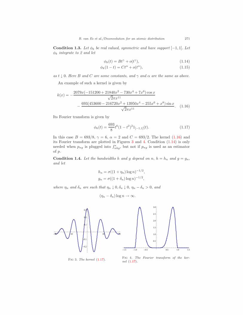
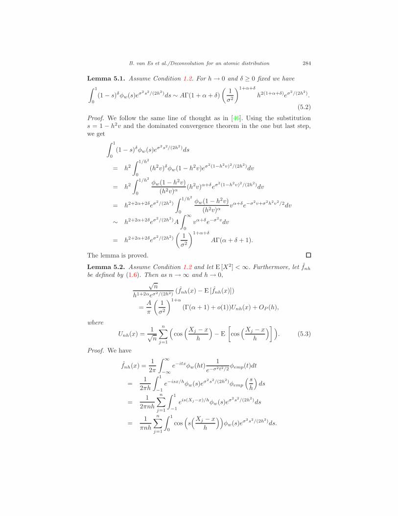
An example of such a kernel is given by

k(x) = −2079x(−151200 + 21840x2 − 730x4 + 7x6) cos x√2πx11

− 693(453600− 216720x2 + 13950x4 − 255x6 + x8) sinx√2πx11

. (1.16)


φk(t) =693

8t6(1 − t2)21[−1,1](t). (1.17)

In this case B = 693/8, γ = 6, α = 2 and C = 693/2. The kernel (1.16) andits Fourier transform are plotted in Figures 3 and 4. Condition (1.14) is onlyneeded when png is plugged into f∗nhg, but not if png is used as an estimatorof p.

Condition 1.4. Let the bandwidths h and g depend on n, h = hn and g = gn,and let

hn = σ((1 + ηn) logn)−1/2,

gn = σ((1 + δn) logn)−1/2,

where ηn and δn are such that ηn ↓ 0, δn ↓ 0, ηn − δn > 0, and

(ηn − δn) logn→ ∞.

-20 -10 10 20

-0.2

-0.1

0.1

0.2

0.3


-1.5 -1.0 -0.5 0.5 1.0 1.5

0.5

1.0

1.5

2.0

2.5

3.0



Furthermore, we assume that

−ηn logn+ (1 + 2α) log logn → ∞,

−δn logn+ (1 + 2α) log logn → ∞.(1.18)

An example of ηn and δn in the definition above is

ηn = 2log log logn

logn, δn =

log log logn

logn.

Conditions on the bandwidths hn and gn in Condition 1.4 are not the onlypossible ones and other restrictions are also possible. However the logarithmicdecay of hn and gn is unavoidable. Following the default convention in kerneldensity estimation and to keep the notation compact, we will suppress the indexn when writing hn and gn and will write h and g instead, since no ambiguitywill arise.

Condition 1.5. Let ǫn ↓ 0 be such that

log ǫn(ηn − δn) logn

→ 0.

An example of such ǫn for ηn and δn given above is (log log logn)−1.The remainder of the paper is organised as follows: in Section 2 we derive

the theorem establishing the asymptotic normality of fnh(x), the fact that theestimator png is weakly consistent, and finally that the estimator f∗nhg(x) isasymptotically normal. Section 3 contains simulation examples. Section 4 dis-cusses a method for implementation of the estimator in practice. All the proofsare collected in Section 5.

2. Main results

We will first study the estimation of f when p is known, and then proceed tothe general case with unknown p. The reason for this is twofold. Firstly, it isinteresting to compare the behaviour of the estimator of f under the assumptionof known and unknown p, and secondly, the proofs of the results for the lattercase rely heavily on the proofs for the former case.

The first result in this section deals with the nonrobustness of the estimatorfnh. In ordinary kernel deconvolution, when it is assumed that Y is absolutelycontinuous, the estimator for its density is defined as

fnh(x) =1

2π

∫ ∞

−∞


e−σ2t2/2dt. (2.1)

Now suppose that the assumption of absolute continuity of Y is violated. Whatwill happen, if we still use the estimator fnh(x)? The following result addressesthis question.


Theorem 2.1. Let fnh(x) be defined as in (2.1). Assume that φw is bounded

and has a compact support on [−1, 1]. Then

E [fnh(x)] = pwh(x) + (1 − p)f ∗ wh(x), (2.2)

where wh(·) = (1/h)w(·/h), and ∗ denotes convolution.

From this theorem it follows that E [fnh(0)] diverges to infinity as h → 0,because so does h−1w(0), if w(0) 6= 0 (the latter is the case for the majority ofconventional kernels). In practice this will also result in an equally undesirable

behaviour of E [fnh(x)] in the neighbourhood of zero. When x 6= 0, with aproper selection of a kernel w, one can achieve that the first term in (2.2)asymptotically vanishes as h → 0. Indeed, it is sufficient to assume that w is suchthat limu→±∞ uw(u) = 0. The second term in (2.2) will converge to (1− p)f(x)as h → 0, provided that φf is integrable, φw is bounded and φw(0) = 1. These

facts address the issue of the nonrobustness of fnh: under a misspecified model,i.e. under the assumption that the distribution of Y is absolutely continuous,while in fact it has an atom at zero, the classical deconvolution estimator willexhibit unsatisfactory behaviour near zero. This will happen despite the factthat fnh(x) will be asymptotically normal when centred at its expectation andsuitably normalised, see Corollary 5.1 in Section 5. The asymptotic normalityfollows from Lemmas 5.2 and 5.3 of Section 5, where only absolute continuityof the distribution of X is required.

Our next goal is to establish the asymptotic normality of the estimatorfnh(x). We formulate the corresponding theorem below.

Theorem 2.2. Assume that φf is integrable. Let E [X2] <∞, and suppose that

Condition 1.2 holds. Let fnh be defined as in (1.4). Then, as n→ ∞ and h→ 0,

√n

h1+2αeσ2/(2h2)(fnh(x) − E [fnh(x)])

D→ N

(

0,A2

2π2(1 − p)2

(

1

σ2

)2+2α

(Γ(α+ 1))2

)

, (2.3)

where Γ denotes the gamma function, Γ(t) =∫∞

0vt−1e−vdv.

Note that Theorem 2.2 establishes asymptotic normality of fnh under anatomic distribution, which constitutes a generalisation of a result in [46] (seealso [45]) for the case of the classical deconvolution problem. The generalisationis possible, because the proof uses only the continuity of the density of X,which is still true when Y has a distribution with an atom. Furthermore, noticethat in order to get a consistent estimator, from this theorem it follows that√nh−1−2αe−σ2/(2h2) has to diverge to infinity. Therefore the bandwidth h has

to be at least of order (logn)−1/2, as it is actually stated in Condition 1.4. Inpractice this implies that the bandwidth h has to be selected fairly large, evenfor large sample sizes. This is the case for the classical deconvolution problemas well in the case of a supersmooth error distribution, cf. [46].


Observe that the asymptotic variance in (2.3) does not depend on the targetdensity f nor on the point x. This phenomenon is quite peculiar, but is alreadyknown in the classical deconvolution kernel density estimation, see for instanceequation (6) in [3]. There, provided that h is small enough, the asymptotic vari-ance of the deconvolution kernel density estimator (or, strictly speaking an upperbound for it) also does not depend neither on the target density f, nor on thepoint x. In this respect see also [46]. Such results do not contradict the asymp-totic normality result in [21], see Theorem 2.2 in that paper, as there the asymp-totic variance of the deconvolution kernel density estimator is not evaluated.

Now we state a theorem concerning the consistency of png, the estimator of p.

Theorem 2.3. Assume that φf is integrable, let E [X2] <∞, and let the kernel

k have a Fourier transform φk that is bounded by one and integrates to two. Let

png be defined as in (1.8). If g is such that g4+4αeσ2/g2

n−1 → 0, then png is a

consistent estimator of p, i.e.

P(|png − p| > ǫ) → 0

as n→ 0 and g → 0. Here ǫ is an arbitrary positive number. Furthermore, under

Condition 1.1 and 1.3

E [(png − p)2] = O

(

g2+2γ +g4+4αeσ2/g2

n

)

.

One can also show that png is asymptotically normal, when centred andsuitably normalised. We formulate the corresponding theorem below.

Theorem 2.4. Assume that the conditions of Theorem 2.3 hold. Let png be

defined as in (1.8) and let (1.15) hold. Then

√n

g2+2αeσ2/(2g2)(png − E [png])

D→ N

(

0,C2(Γ(1 + α))2

2

(

1

σ2

)2+2α)

as n → ∞ and g → 0.

Finally, we consider the case when both p and f are unknown. We state themain theorem of the paper.

Theorem 2.5. Let f∗nhg(x) be defined by (1.9), E [X2] < ∞ and let Condi-

tions 1.1–1.5 hold. Then, as n → ∞, we have

√n

h1+2αeσ2/(2h2)(f∗nhg(x) − E [f∗nhg(x)])

D→ N

(

0,A2

2π2(1 − p)2

(

1

σ2

)2+2α

(Γ(α+ 1))2

)

.

Notice that the asymptotic variance is the same as in (2.3), which justifies theplug-in approach to the construction of an estimator of f, when p is unknown.


A natural question to consider is what happens when we centre f∗nhg(x) notat its expectation, but at f(x). This has practical importance as well, e.g. forthe construction of (asymptotic) confidence intervals. Writing

√n

h1+2αeσ2/(2h2)(f∗nhg(x) − f(x)) =

√n


+

√n

h1+2αeσ2/(2h2)(E [f∗nhg(x)]− f(x)),

we see, that we have to study the second term here, i.e. to compare the be-haviour of the bias of f∗nhg(x) to the normalising factor

√nh−(1+2α)e−σ2/(2h2).

We will study the bias of f∗nhg(x) in two steps: first we will show that itasymptotically vanishes, which itself is of independent interest. After this wewill provide conditions under which it asymptotically vanishes when multipliedby

√nh−(1+2α)e−σ2/(2h2). Recall the definition of a Holder class of functions

H(β, L).

Definition 2.1. A function f is said to belong to the Holder class H(β, L), if

its derivatives up to order l = [β] exist and verify the condition

|f(l)(x+ t) − f(l)(x)| ≤ L|t|β−l

for all x, t ∈ R.

Such a smoothness condition on a target density f is standard in kerneldensity estimation, see e.g. p. 5 of [40]. Often one assumes that β = 2. If l = 0,then set f(l) = f. We also need the definition of a kernel of order l. In particular,we will use the version given in Definition 1.3 of [40].

Definition 2.2. A kernel w is said to be a kernel of order l for l ≥ 1, if the

functions x 7→ xjw(x) are integrable for j = 0, . . . , l and if∫ ∞

−∞

w(x)dx = 1,

∫ ∞

−∞

xjw(x)dx = 0 for j = 1, . . . , l.

Theorem 2.6. Let f∗nhg(x) be defined by (1.9) and assume conditions of The-

orem 2.5. Then, as n→ ∞, we have

E [f∗nhg(x)]− f(x) → 0.

If additionally f ∈ H(β, L), w is a kernel of order l = [β] and β > 1 + 2α, then√n

h1+2αeσ2/(2h2)(E [f∗nhg(x)] − f(x)) → 0

as n → ∞.

Combination of this theorem with Theorem 2.5 leads to the following result.

Theorem 2.7. Assume that the conditions of Theorem 2.6 hold. Then, as n→∞, we have

√n

h1+2αeσ2/(2h2)(f∗nhg(x)− f(x))

D→ N

(

0,A2

2π2(1 − p)2

(

1

σ2

)2+2α

(Γ(α+ 1))2

)

.


One should keep in mind that these results deal only with asymptotics. Inthe next section we will study several simulation examples, which will providesome insight into the finite sample properties of the estimator.

3. Simulation examples

In this section we consider a number of simulation examples. We do not pretendto provide an exhaustive simulation study, rather an illustration, which requiresfurther verification.

Assume that σ = 1, p = 0.1 and that f is normal with mean 3 and variance 9.This results in a nontrivial deconvolution problem, because the ratio of ‘noise’compared to ‘signal’ is reasonably high: NSR = Var[σZ]/Var[Y ]100% ≈ 11%.We have simulated a sample of size n = 1000. As kernels w and k we selectedkernels (1.12) and (1.16), respectively. The bandwidths h = 0.58 and g = 0.5were selected by hand. A possible method of computing the estimate is givenin Section 4. The estimator png produced a value equal to 0.11. The estimateof f (bold dotted line), resulting from the procedure described above, togetherwith the target density f (dashed line) is plotted in Figure 5. For comparisonpurposes, we have also plotted the estimate fnh(x) (it can be obtained using(1.5) and the true value of the parameter p), see Figure 6. As can be seen fromthe comparison of these two figures, the estimates f∗nhg and fnh look rathersimilar.

As the second example we consider the case when f is a gamma density withparameters α = 8 and β = 1, i.e.

f(x) =x7e−x

Γ(8)1[x>0], (3.1)

and p = 0.25. We simulated a sample of size n = 1000. The kernels were chosenas above and the bandwidths g = 0.6 and h = 0.6 were selected by hand. Theestimate png took a value approximately equal to 0.23. The resulting estimate

-5 5 10 15

0.02

0.04

0.06

0.08

0.10

0.12

0.14

Fig 5. The normal density f (dashed line)and the estimate f∗

nhg(solid line). The

sample size n = 1000.

-5 5 10 15

0.02

0.04

0.06

0.08

0.10

0.12

0.14

Fig 6. The normal density f (dashed line)and the estimate fnh (solid line). The sam-ple size n = 1000.


-5 5 10 15 20

0.02

0.04

0.06

0.08

0.10

0.12

0.14

Fig 7. The gamma density (dashed line)and the estimate f∗

nhg(solid line). The

sample size n = 1000.

-5 5 10 15 20

0.05

0.10

0.15

Fig 8. The gamma density (dashed line)and the estimate fnh (solid line). The sam-ple size n = 1000.

-0.05 0 0.05 0.1 0.15 0.2 0.25

20

40

60

80

Fig 9. The histogram of estimates of p forg = 0.5 and the sample size n = 1000.

0 0.05 0.1 0.15 0.2 0.25

20

40

60

80

100


f∗nhg is plotted in Figure 7. As above we also plotted the estimate fnh, seeFigure 8 (notice that the estimate takes on negative values in the neighbourhoodof zero). Again both figures look similar.

Examination of these figures leads us to two questions: how well does png

estimate p for moderate sample samples? How sensitive is f∗nhg to under- oroverestimation of p? To get at least a partial answer to the first question, weconsidered the same model as in our first example in this section (i.e. decon-volution of the normal density) and repeatedly, i.e. 1000 times, estimated p forthe bandwidth g = 0.5 and the sample size n = 1000 for each simulation run.Then the same procedure was repeated for the bandwidths g = 0.55, 0.6 and0.65. The resulting histograms are plotted in Figures 9–12. They look quite sat-isfactory. The sample means and sample standard deviations (SD) of estimatesof p for different choices of bandwidth g together with the theoretical standarddeviations are summarised in Table 1. One notices that the sample means in Ta-ble 1 are close to the true value 0.1 of the parameter p. The theoretical standarddeviations in the same table were computed using Theorem 2.4, which predicts


0 0.05 0.1 0.15 0.2

10

20

30

40

50

60


0 0.05 0.1 0.15 0.2

20

40

60

80

100

120

140


Table 1

Sample and theoretical means and standard deviations (SD) of estimates of p for differentchoices of bandwidth g. The sample size n = 1000

Bandwidth 0.5 0.55 0.6 0.65Sample mean 0.0963 0.0975 0.0960 0.0927

Sample SD 0.0516 0.0436 0.0388 0.0349Asymptotic SD 1.7891 2.2399 2.8994 3.8164Theoretical SD 0.0700 0.0593 0.0487 0.0432

that they should be equal to (recall, that in our case α = 2)

g6e1/(2g2)

√n

C√

2.

From Table 1 one sees that there is a large discrepancy between the samplestandard deviations and the standard deviations predicted by the theory. Theexplanation of this discrepancy lies in the fact that the proof of the asymptoticnormality of png heavily relies on the asymptotic equivalence

∫ 1

0

φk(s)eσ2s2/(2g2)ds ∼ CΓ(1 + α)

(

1

σ2

)1+α

g2(1+α)eσ2/(2g2), (3.2)

see Lemma 5.1 and the proof of Lemma 5.2 in Section 5 below. However, bydirect evaluation of the integral on the left-hand side of (3.2) for different valuesof g, it can be seen that this relation does not provide an accurate approximationin those cases where the bandwidth is relatively large, as it actually is in ourcase. It then follows that the asymptotic standard deviation will not providea good approximation of the sample standard deviation unless the bandwidthis very small. This in turn implies that the corresponding sample size mustbe extremely large. We can correct for this poor approximation of the integralin (3.2) by using the integral itself as a normalising factor instead of the right-hand side of (3.2). The results of this correction are represented in the lastline of Table 1. As it can be seen, the theoretical standard deviation and thesample standard deviation are much closer to each other. Since the kernel k was


-10 -5 5 10

0.02

0.04

0.06

0.08

0.10

0.12

0.14


-1.5 -1.0 -0.5 0.5 1.0 1.5

0.2

0.4

0.6

0.8

1.0


selected more or less arbitrarily, one is tempted to believe that an inaccurateapproximation in (3.2) might be due to the kernel. This might be the case,however to a certain degree this seems to be characteristic of all popular kernelsemployed in kernel deconvolution. Consider for instance the kernel

w(x) =48x(x2 − 15) cosx− 144(2x2 − 5) sinx

πx7. (3.3)


φw(t) = (1 − t2)31[|t|<1].

The kernel w and its Fourier transform are plotted in Figures 13 and 14, respec-tively. This kernel was used for simulations in [22] and [47] and it was shown in[13] that it performs well in a deconvolution setting. Notice that this kernel can-not be used to estimate p if we want to plug in the resulting estimator png intof∗nhg . However, this kernel satisfies Condition 1.2 and can be used to estimatef. Nevertheless, the ratio of the left and right hand sides in (3.2) for h = 0.5 isequal to 0.4299, which is still far from 1. This issue is further discussed in [42].Another issue here is that often the error variance σ2 is quite small and it is sen-sible to treat σ as depending on the sample size n (with σ → 0 as n→ ∞), see[9]. However, this is a different model and this question is not addressed here.Notice also that a perfect match between the sample standard deviation andthe theoretical standard deviation is impossible to obtain, because we neglect aremainder term when computing the latter. How large the contribution of theremainder term can be in general requires a separate simulation study.

We also considered the case when the error term variance and the sample sizeare smaller (the target density f was again the standard normal density, while pwas set to be 0.1). In particular, we took σ = 0.3 and n = 500. The correspond-ing histograms are given in Figures 15–18, while the sample and theoreticalcharacteristics for four different choices of the bandwidth g = 0.5, 0.55, 0.6 and0.65 are summarised in Table 2. Notice a particularly bad match between theasymptotic standard deviation and its empirical counterpart. Other conclusionsare similar to those in the previous example.


0.05 0.1 0.15

10

20

30

40

50

60

70


0.025 0.05 0.075 0.1 0.125 0.15 0.175

20

40

60


0.05 0.1 0.15

20

40

60

80


0.025 0.05 0.075 0.1 0.125 0.15 0.175

20

40

60

80


To test the robustness of the estimator f∗nhg with respect to the estimatedvalue of p, we again turned to the model that was considered in the first exampleof this section. Instead of png three different values p = 0.05, p = 0.1 andp = 0.15 were plugged in into (4.2). The resulting estimates f∗nhg are plotted inFigure 19 (the true density is represented by the dashed line). As one can seefrom Figure 19, under- or overestimation of p in the given range does not havea significant impact on the resulting estimate fnh (of course one should keep inmind that p is relatively small in this case). On the other hand, if the value ofp were larger, e.g. if p = 0.2, that would have a noticeable effect, e.g. it couldhave suggested bimodality in the case where the density is actually unimodal,see Figure 20 on the facing page. At the same time the simulated examplesconcerning the estimates png that we considered above seem to suggest thatsuch instances of unsatisfactory estimates of p are not too frequent, becausemost of the observed values of png are concentrated in the interval [0.05, 0.15].We also considered the case when f = 0.5φ−2,1+0.5φ2,1, where φx,y denotes thenormal density with mean x and variance y. Hence in this case f is a mixtureof two normal densities and it is also bimodal. The match is visually slightlyworse for p = 0.2, but it is still acceptable.


Table 2

Sample and theoretical means and standard deviations (SD) of estimates of p for differentchoices of bandwidth g. The sample size n = 500

Bandwidth 0.45 0.5 0.6 0.65Sample mean 0.0972 0.0977 0.0959 0.0930

Sample SD 0.0277 0.0269 0.0283 0.0295Asymptotic SD 311.7 562.3 2247 2521Theoretical SD 0.0357 0.0349 0.0338 0.0335

-5 5 10 15

0.02

0.04

0.06

0.08

0.10

0.12

0.14

Fig 19. The normal density f and esti-mates f∗

nhgevaluated for p = 0.05, p = 0.1,

p = 0.15 and the sample size n = 1000.

-5 5 10 15

0.02

0.04

0.06

0.08

0.10

0.12

0.14

Fig 20. The normal density f and estimatef∗

nhgevaluated for p = 0.2 and the sample

size n = 1000.

The simulation examples that we considered in this section suggest that,despite the slow (logarithmic) rate of convergence, the estimator f∗nhg works inpractice (given that p is estimated accurately). This is somewhat comparable tothe classical deconvolution problem, where by finite sample calculations it wasshown in [47] that for lower levels of noise, the kernel estimators perform well forreasonable sample sizes, in spite of slow rates of convergence for the supersmoothdeconvolution problem, obtained e.g. in [21] and [22]. However, Condition 1.4tells us, that the bandwidths h and g have to be of order (logn)−1/2. In practicethis implies that to obtain reasonable estimates, the bandwidths have to beselected fairly large, even for large samples.

One more practical issue concerning the implementation of the estimatorf∗nhg (or png) is the method of bandwidth selection, which is not addressed inthis paper. We expect that techniques similar to those used in the classicaldeconvolution problem will produce comparable results in our problem. Thisrequires a separate investigation of the behaviour of the mean integrated squareerror of f∗nhg . In the case of the classical deconvolution problem papers thatconsider the issue of data-dependent bandwidth selection are [10, 11, 18, 28]and [39]. Yet another issue is the choice of kernels w and k. For the case ofthe classical deconvolution problem we refer to [13]. In general in kernel densityestimation it is thought that the choice of a kernel is of less importance for theperformance of an estimator than the choice of the bandwidth, see e.g. p. 31 in[48], or p. 132 in [49].


-5 5

0.05

0.10

0.15

0.20

Fig 21. The mixture of normal densities f

and estimates f∗nhg

evaluated for p = 0.05,

p = 0.1, p = 0.15. and the sample size n =1000.

-5 5

0.05

0.10

0.15

0.20

Fig 22. The mixture of normal densities f

and estimate f∗nhg

evaluated for p = 0.2

and the sample size n = 1000.

4. Computational issues

To compute the estimator f∗nhg in Section 3, a method similar to the one usedin [44] (in turn motivated by [5]) can be employed. Namely, notice that

fnh(x) = f(1)nh (x) + f

(2)nh (x),

where

f(1)nh (x) =

1

2π

∫ ∞

0


e−σ2t2/2dt,

f(2)nh (x) =

1

2π

∫ ∞

0

eitxφemp(−t)φw(ht)

e−σ2t2/2dt.

Using the trapezoid rule and setting vj = η(j − 1), we have

f(1)nh (x) ≈ 1

2π

N∑

j=1

e−ivjxψ(vj)η, (4.1)

where N is some power of 2 and

ψ(vj) =φemp(vj)φw(hvj)

e−σ2v2

j/2

.

The Fast Fourier Transform is used to compute values of f(1)nh at N different

points (concerning the application of the Fast Fourier Transform in kernel de-convolution see [12]). We employ a regular spacing size δ, so that the values ofx are

xu = −Nδ2

+ δ(u− 1),

where u = 1, . . . , N. Therefore, we obtain

f(1)nh (xu) ≈ 1

2π

N∑

j=1

e−iδη(j−1)(u−1)eivjNδ2 ψ(vj)η.


In order to apply the Fast Fourier Transform, note that we must take

δη =2π

N.

It follows that a small η, which is needed to achieve greater accuracy in integra-tion, will result in values of x which are relatively far from each other. Therefore,to improve the integration precision, we will apply Simpson’s rule, i.e.

f(1)nh (xu) ≈ 1

2π

N∑

j=1

e−i 2πN

(j−1)(u−1)eivjNδ2 ψ(vj)

η

3(3 + (−1)j − δj−1),

where δj denotes the Kronecker symbol (recall, that δj is 1, if j = 0 and is 0

otherwise). The same reasoning can be applied to f(2)nh (x). The estimate f∗nhg

can then be computed by noticing that

f∗nhg(x) =fnh(x)

1 − png− png

1 − pngwh(x). (4.2)

One should keep in mind that even though wh can be evaluated directly, it ispreferable to use the Fast Fourier Transform for its computation, thus avoidingpossible numerical issues, see [12]. Also notice that the direct computation ofφemp is rather time-demanding for large samples. One way to avoid this problemis to use WARPing, cf. [27]. However, for the purposes of the present study, werestricted ourselves to the direct evaluation of φemp.

5. Proofs

Proof of Theorem 2.1. The proof is elementary and is based on the definitionof fnh(x). By Fubini’s theorem we have

E

[

1

2π

∫ ∞

−∞


e−σ2t2/2dt

]

=1

2π

∫ ∞

−∞

e−itxφY (t)φw(ht)dt.

Recalling that φY (t) = p+ (1 − p)φf(t), we obtain

E [fnh(x)] = pwh(x) + (1 − p)f ∗ wh(x). (5.1)

Here we used the facts that

1

2π

∫ ∞

−∞

e−itxφw(ht)dt = wh(x),

1

2π

∫ ∞

−∞

e−itxφf(t)φw(ht)dt = f ∗ wh(x).

This concludes the proof.

The proof of Theorem 2.2 is based on the following three lemmas, all of whichare reformulations of results from [46].


Lemma 5.1. Assume Condition 1.2. For h→ 0 and δ ≥ 0 fixed we have

∫ 1

0

(1 − s)δφw(s)eσ2s2/(2h2)ds ∼ AΓ(1 + α+ δ)

(

1

σ2

)1+α+δ

h2(1+α+δ)eσ2/(2h2).

(5.2)

Proof. We follow the same line of thought as in [46]. Using the substitutions = 1 − h2v and the dominated convergence theorem in the one but last step,we get

∫ 1

0

(1 − s)δφw(s)eσ2s2/(2h2)ds

= h2

∫ 1/h2

0

(h2v)δφw(1 − h2v)eσ2(1−h2v)2/(2h2)dv

= h2

∫ 1/h2

0

φw(1 − h2v)

(h2v)α(h2v)α+δeσ2(1−h2v)2/(2h2)dv

= h2+2α+2δeσ2/(2h2)

∫ 1/h2

0

φw(1 − h2v)

(h2v)αvα+δe−σ2v+σ2h2v2/2dv

∼ h2+2α+2δeσ2/(2h2)A

∫ ∞

0

vα+δe−σ2vdv

= h2+2α+2δeσ2/(2h2)

(

1

σ2

)1+α+δ

AΓ(α + δ + 1).

The lemma is proved.

Lemma 5.2. Assume Condition 1.2 and let E [X2] <∞. Furthermore, let fnh

be defined by (1.6). Then as n → ∞ and h→ 0,√n


=A

π

(

1

σ2

)1+α

(Γ(α + 1) + o(1))Unh(x) +OP (h),

where

Unh(x) =1√n

n∑

j=1

(

cos(Xj − x

h

)

− E

[

cos(Xj − x

h

)

]

)

. (5.3)

Proof. We have

fnh(x) =1

2π

∫ ∞

−∞

e−itxφw(ht)1

e−σ2t2/2φemp(t)dt

=1

2πh

∫ 1

−1

e−isx/hφw(s)eσ2s2/(2h2)φemp

( s

h

)

ds

=1

2πnh

n∑

j=1

∫ 1

−1

eis(Xj−x)/hφw(s)eσ2s2/(2h2)ds

=1

πnh

n∑

j=1

∫ 1

0

cos(

s(Xj − x

h

))

φw(s)eσ2s2/(2h2)ds.


Notice that

cos(

s(Xj − x

h

))

= cos(Xj − x

h

)

+(

cos(

s(Xj − x

h

))

− cos(Xj − x

h

))

= cos(Xj − x

h

)

− 2 sin(1

2(s+ 1)

(Xj − x

h

))

sin(1

2(s− 1)

(Xj − x

h

))

= cos(Xj − x

h

)

+Rn,j(s),

where Rn,j(s) is a remainder term satisfying

|Rn,j| ≤ (|x|+ |Xj|)(1 − s

h

)

, 0 ≤ s ≤ 1. (5.4)

The bound follows from the inequality | sinx| ≤ |x|.By Lemma 5.1, fnh(x) equals

1

πh

∫ 1

0

φw(s)eσ2s2/(2h2)ds1

n

n∑

j=1

cos(Xj − x

h

)

+1

n

n∑

j=1

Rn,j

=A

π(Γ(α+ 1) + o(1))

(

1

σ2

)1+α

h1+2αeσ2/(2h2) 1

n

n∑

j=1

cos(Xj − x

h

)

+1

n

n∑

j=1

Rn,j,

where

Rn,j =1

π

1

h

∫ 1

0

Rn,j(s)φw(s)eσ2s2/(2h2)ds.

For the remainder we have, by (5.4) and Lemma 5.1,

|Rn,j| ≤1

π(|x|+ |Xj|)

1

h

∫ 1

0

(1 − s

h

)

φw(s)eσ2s2/(2h2)ds

=A

π(|x| + |Xj|)(Γ(α+ 2) + o(1))h2+2α

(

1

σ2

)2+α

eσ2/(2h2).

Consequently,

Var[

Rn,j

]

≤ E[

R2n,j

]

= O(

h4+4αeσ2/h2)

and1

n

n∑

j=1

(Rn,j − E[

Rn,j

]

) = OP

(h2+2α

√neσ2/(2h2)

)

,

which follows from Chebyshev’s inequality. Finally, we get√n


=A

π(Γ(α+ 1) + o(1))

(

1

σ2

)1+α

Unh(x) + OP (h),

and this completes the proof of the lemma.


The next lemma establishes the asymptotic normality.

Lemma 5.3. Assume conditions of Lemma 5.2 and let, for a fixed x, Unh(x)be defined by (5.3). Then, as n→ ∞ and h → 0,

Unh(x)D→ N

(

0,1

2

)

.

Proof. Write

Yj =Xj − x

hmod 2π.

For 0 ≤ y < 2π we have

P (Yj ≤ y) =

∞∑

k=−∞

P (2kπh+ x ≤ Xj ≤ 2kπh+ yh + x)

=

∞∑

k=−∞

∫ 2kπh+yh+x

2kπh+x

q(u)du =

∞∑

k=−∞

yh q(ξk,h)

=y

2π

∞∑

k=−∞

2πh q(ξk,h) ∼ y

2π

∫ ∞

−∞

q(u)du =y

2π,

where ξk,h is a point in the interval [2kπh+x, 2kπh+yh+x] ⊂ [2kπh+x, 2(k+1)πh+x]. Since h→ 0, the last equivalence follows from a Riemann sum approx-imation of the integral and continuity of the density q of X. Consequently, as

h → 0, we have YjD→ U, where U is uniformly distributed on the interval [0, 2π].

Since the cosine is bounded and continuous, it then follows by the dominatedconvergence theorem that E [| cosYj |a] → E [| cosU |a], for all a > 0. Therefore

E

[

cos

(

Xj − x

h

)]

→ E [cosU ] = 0

and

E

[

(

cos

(

Xj − x

h

))2]

→ E [(cosU)2] =1

2.

To prove asymptotic normality of Unh(x), first note that it is a normalisedsum of i.i.d. random variables. We will verify that the conditions for asymptoticnormality in the triangular array scheme of Theorem 7.1.2 in [8] hold (Lya-punov’s condition). In our case this reduces to the verification of the fact that

n∑

j=1

E [| cosYj − E [cosYj]|3]n3/2(Var[cosYj ])3/2

=E [| cosY1 − E [cosY1]|3]n1/2(Var[cosY1])3/2

→ 0.

Now notice that

E [| cosY1 − E [cosY1]|3]n1/2(Var[cosY1])3/2

∼ E [| cosU |3]n1/2(Var[cosU ])3/2

→ 0,


as n → ∞. Consequently, Unh is asymptotically normal,

Unh(x)D→ N

(

0,1

2

)

.

The following corollary immediately follows from Lemmas 5.2 and 5.3.

Corollary 5.1. Under the conditions of Lemma 5.2 we have that

√n

h1+2αeσ2/(2h2)

(

fnh(x) − E [fnh(x)])

D→ N

(

0,A2(Γ(α + 1))2

2π2

(

1

σ2

)2+2α)

.

Now we prove Theorem 2.2.

Proof of Theorem 2.2. From (1.4) we have that

fnh(x) − E[fnh(x)] =1

1 − p(fnh(x) − E[fnh(x)]).

Hence the result follows from Corollary 5.1.

The following lemma gives the order of the variance of fnh(x).

Lemma 5.4. Let Condition 1.2 hold and fnh(x) be defined as in (1.4). Then,

as n → ∞ and h→ 0,

Var[fnh(x)] = O

(

h2(1+2α)eσ2/h2

n

)

.

Proof. We have

Var[fnh(x)] =1

4π2(1 − p)21

nh2Var

[∫ 1

−1

eis(X1−x)/hφw(s)eσ2s2/(2h2)ds

]

.

Notice that

Var

[∫ 1

−1

eis(X1−x)/hφw(s)eσ2s2/(2h2)ds

]

≤(

2

∫ 1

0

|φw(s)|eσ2s2/(2h2)ds

)2

.

Recalling Lemma 5.1, we conclude that

Var[fnh(x)] = O

(

h2(1+2α)eσ2/h2

n

)

.

Next we deal with consistency of png and prove Theorem 2.3.

Proof of Theorem 2.3. We have

png − p = (png − E [png]) + (E [png] − p).


To prove that this expression converges to zero in probability, it is sufficient toprove that Var[png] → 0 and E [png] − p → 0 as n → ∞, g → 0. We have

Var[png] = π2g2 Var

[

1

2π

∫ 1/g

−1/g

φemp(t)φk(gt)

e−σ2t2/2dt

]

= π2g2 Var[fng(0)].

Here it is understood that replacing subindex h by g entails replacement of thesmoothing characteristic function φw by φk. By Lemma 5.4,

Var[png] = O

(

g4+4αeσ2/g2

n

)

. (5.5)

This converges to zero due to the condition on g. Furthermore,

E [pnh] − p = p

(

1

2

∫ 1

−1

φk(t)dt− 1

)

+ (1 − p)g

2

∫ 1/g

−1/g

φf (t)φk(gt)dt. (5.6)

The first term here is zero, since φk integrates to 2, while the second termconverges to zero, which can be seen upon noticing that φk is bounded, φf isintegrable and that this term is bounded by

1 − p

2g

∫ ∞

−∞

|φf(t)|dt,

which converges to zero as g → 0. The last part of the theorem follows from theidentity

∫ 1/g

−1/g

φf(t)φk(gt)dt = gγ

∫ 1/g

−1/g

tγφf(t)φk(gt)

(gt)γdt

and Conditions 1.1 and 1.3, because Condition 1.3 implies the existence of aconstant K, such that supt |φk(t)t

−γ | < K.

Next we prove asymptotic normality of png.

Proof of Theorem 2.4. The result follows from the definition of png and Corol-

lary 5.1, because png = gπfng(0) essentially is a rescaled version of fng(0).

Now we are ready to prove Theorem 2.5.

Proof of Theorem 2.5. Write

√n


=

√n

h1+2αeσ2/(2h2)

(

1

1 − png

1

2π

∫ ∞

−∞


e−σ2t2/2dt

− E

[

1

1 − png

1

2π

∫ ∞

−∞


e−σ2t2/2dt

])

−√n

h1+2αeσ2/(2h2)

1

hw(x

h

)

(

png

1 − png− E

[

png

1 − png

])

. (5.7)


We want to prove that the first term is asymptotically normal, while the sec-ond term converges to zero in probability. Application of Slutsky’s lemma, seeLemma 2.8 in [41], will then imply that the above expression is asymptoticallynormal.

First we deal with the second term. We have√n

h2+2αeσ2/(2h2)w(x

h

)

(

png

1 − png− E

[

png

1 − png

])

= w(x

h

)

( √n

h2+2αeσ2/(2h2)

g2+2αeσ2/(2g2)

√n

)

×√n

g2+2αeσ2/(2g2)

(

png

1 − png− E

[

png

1 − png

])

. (5.8)

Note that Condition 1.4 implies

√n

h2+2αeσ2/(2h2)

g2+2αeσ2/(2g2)

√n

=

(

1 + ηn

1 + δn

)1+α

exp

(

1

2(δn − ηn) logn

)

→ 0.

Next we prove that√n

g2+2αeσ2/(2g2)

(

png

1 − png− E

[

png

1 − png

])

(5.9)

is asymptotically normal. Then (5.8) will converge to zero in probability, sinceconvergence to a constant in distribution is equivalent to convergence to thesame constant in probability and because w is bounded. We have

√n


D→ N

(

0,C2(Γ(1 + α))2

2

(

1

σ2

)2+2α)

, (5.10)

which can be seen as follows:√n

g2+2αeσ2/(2g2)(png − E [png]) =

√n


+

√n

g2+2αeσ2/(2g2)(png − png − E [png − png]).

Due to Theorem 2.4 the first term here yields the asymptotic normality. Wewill prove that the second term converges to zero in probability. To this end itis sufficient to prove that

Var

[ √n

g2+2αeσ2/(2g2)(png − png)

]

=n

g4+4αeσ2/g2Var [png − png] → 0. (5.11)

It follows from the definition of png and Lemma 5.1 that

Var [png − png] ≤ E [(1 − εn − png)21[png>1−ǫn]]

≤ (2 + 2K2g4(1+α)eσ2/g2

) P(png > 1 − εn), (5.12)


where K is some constant. This and (5.11) imply that we have to prove

nP(png > 1 − εn) → 0. (5.13)

NowP(png > 1 − ǫn) = P(png − E [png] > 1 − ǫn − E [png]). (5.14)

Denote tn ≡ 1 − ǫn − E [png] and select n0 so large that for n ≥ n0, we havetn > 0. Notice that tn → 1 − p, which follows from (5.6). The probabilityin (5.14) is bounded by P(|png − E [png]| > tn). Note that

png =

n∑

j=1

1

nπkg

(−Xj

g

)

,

with

kg(x) =1

2π

∫ 1

−1

e−itxφk(t)eσ2t2/(2g2)dt.

By Lemma 5.1, which is applicable in view of Condition 1.3,

1

nπkg

(−xg

)

(5.15)

is bounded by a constant K, say, times g2+2αeσ2/(2g2)n−1. Hoeffding’s inequality,see [29], then yields

P(|png − E [png]| > tn) ≤ 2 exp

(

−2t2nK2

n

g2(2+2α)eσ2/g2

)

. (5.16)

Since now

nP(|png − E [png]| > tn) ≤ 2n exp

(

−2t2nK2

n

g2(2+2α)eσ2/g2

)

,

it is enough to prove that the term on the right-hand side converges to zero.Taking the logarithm yields

log 2 + logn− 2t2nK2

n

g2(2+2α)eσ2/g2.

This diverges to minus infinity, because the last term dominates logn,

n

g2(2+2α)eσ2/g2

1

logn→ ∞.

The latter fact can be seen by taking the logarithm of the left-hand side andusing (1.18). We obtain

logn− (2 + 2α) log g2 − σ2

g2− log logn

= −δn logn+ (1 + 2α) log logn− (2 + 2α) logσ2 +(2 + 2α) log(1 + δn) → ∞,


which follows from (1.18). This in turn proves that (5.10) is asymptoticallynormal. Since the derivative (y/(1−y))′ 6= 0, a minor variation of the δ-methodthen implies that (5.9) is also asymptotically normal (see Theorem 3.8 in [41]for the δ-method). Consequently, the second term in (5.7) converges to zero inprobability.

We now consider the first term in (5.7) and want to prove that it is asymp-totically normal. Rewrite this term as

√n

h1+2αeσ2/(2h2)

(

1

1 − p

1

2π

∫ ∞

−∞


e−σ2t2/2dt

− E

[

1

1 − p

1

2π

∫ ∞

−∞


e−σ2t2/2dt

])

+

√n

h1+2αeσ2/(2h2)

({

1

1 − png− 1

1 − p

}

1

2π

∫ ∞

−∞


e−σ2t2/2dt

− E

[{

1

1 − png− 1

1 − p

}

1

2π

∫ ∞

−∞


e−σ2t2/2dt

])

.

Thanks to Corollary 5.1 the first summand here is asymptotically normal. Wewill prove that the second term vanishes in probability. Due to Chebyshev’sinequality, it is sufficient to study the behaviour of

√n

h1+2αeσ2/(2h2)E

[∣

∣

∣

∣

png − p

(1 − png)(1 − p)

1

2π

∫ ∞

−∞


e−σ2t2/2dt

∣

∣

∣

∣

]

.

By the Cauchy-Schwarz inequality, after taking squares, we can instead consider

n

h2(1+2α)eσ2/h2E

[

(png − p)2

(1 − png)2(1 − p)2

]

× E

[

(

1

2π

∫ ∞

−∞


e−σ2t2/2dt

)2]

. (5.17)

Notice that

E

[

(

1

2π

∫ ∞

−∞


e−σ2t2/2dt

)2]

= Var

[

1

2π

∫ ∞

−∞


e−σ2t2/2dt

]

+

(

E

[

1

2π

∫ ∞

−∞


e−σ2t2/2dt

])2

.

It is easy to see that this expression is of order h−2. Indeed, due to Lemma 5.4the first term in this expression is of order n−1h2(1+2α)eσ2/h2

. The fact thatthis in turn is of lower order than h−2 can be seen in the same way as we did


with (5.6). For the second term we have

(

E

[

1

2π

∫ ∞

−∞


e−σ2t2/2dt

])2

=

(

p

hw(x

h

)

+ (1 − p)1

2π

∫ ∞

−∞

e−itxφf (t)φw(ht)dt

)2

,

and this is of order h−2, because

∣

∣

∣

∣

(1 − p)1

2π

∫ ∞

−∞

e−itxφf(t)φw(ht)dt

∣

∣

∣

∣

≤ (1 − p)1

2π

∫ ∞

−∞

|φf(t)|dt

and because w is bounded. Consequently, taking into account (5.17), we haveto study

n

h4+4αeσ2/h2E

[

(png − p)2

(1 − png)2(1 − p)2

]

,

or1

(1 − p)2n

ǫ2nh2(2+2α)eσ2/h2

E [(png − p)2], (5.18)

since (1 − png)−2 ≤ ǫ−2

n . Now

E [(png − p)2] ≤ 2E [(png − png)2] + 2E [(png − p)2].

Hence we have to prove that

n


E [(png − png)2] → 0, (5.19)

n


E [(png − p)2] → 0. (5.20)

The first fact essentially follows from the arguments concerning (5.11), sincethe presence of an additional factor ǫ−2

n given Condition 1.5 does not affect thearguments used. Indeed, (5.19) will hold true, if we prove that

1

ǫ2n

n

h4+4αeσ2/h2g4+4αeσ2/g2

P(png > 1 − ǫn) → 0.

Here we used the definitions of png and png and Lemma 5.1. Now notice that(g/h)4+4α → 1, which follows from Condition 1.4 and that by arguments con-cerning (5.13) we have nP(png > 1 − ǫn) → 0. Moreover, under Conditions 1.4

and 1.5 we have ǫ−2n eσ2/2(1/g2−1/h2) → 0, which can again be seen by taking the

logarithm and verifying that it diverges to minus infinity. This proves (5.19).Next we will prove (5.20). Notice that the latter is in turn implied by

n


Var[png] +n


(E [png − p])2 → 0.


The first term here converges to zero by (5.5) and Conditions 1.4 and 1.5. Nowwe turn to the second term. Taking into account (5.6), we have to study thebehaviour of √

n

ǫnh2+2αeσ2/(2h2)(1 − p)

∫ 1

−1

φf

(

t

g

)

φk(t)dt.

This can be rewritten as( √

n

ǫnh2+2αeσ2/(2h2)

g2+2αeσ2/(2g2)

√n

) √n

g2+2αeσ2/(2g2)

∫ 1

−1

φf

(

t

g

)

φk(t)dt.

The factor between the brackets in this expression converges to zero. Thereforeit is sufficient to consider

√n

g2+2αeσ2/(2g2)

∫ 1

−1

φf

(

t

g

)

φk(t)dt.

Rewrite this as

√n

g1+2αeσ2/(2g2)gγ

∫ 1/g

−1/g

tγφf(t)φk(gt)

(gt)γdt.

Conditions 1.1, 1.3, 1.4 and 1.5 imply that this expression converges to zero,because the integral converges to a constant by the dominated convergencetheorem, while √

n

g1+2αeσ2/(2g2)gγ → 0,

which can be seen by taking the logarithm and noticing that it diverges to minusinfinity. We obtain

1

2logn+ (γ − 1 − 2α) log g − σ2

2g2= −δn

2logn+ (γ − 1 − 2α) logσ

+1 + 2α− γ

2log(1 + δn) +

1 + 2α− γ

2log logn

≤ (γ − 1 − 2α) logσ

+1 + 2α− γ

2log(1 + δn) +

1 + 2α− γ

2log logn → −∞, (5.21)

which follows from the facts that δn > 0 and 1 + 2α − γ < 0. Combination ofall these intermediary results completes the proof of the theorem.

Proof of Theorem 2.6. Write

E [f∗nhg(x)] − f(x) = {E[f∗nhg(x) − fnh(x)]}+ {E [fnh(x)]− f(x)}. (5.22)

Because of (1.7), the second summand in this expression vanishes as h → 0.Next we consider the first summand in (5.22). Using the definitions of f∗nhg(x)


and fnh(x), we get

E [f∗nhg(x) − fnh(x)] = E

[

png − p

(1 − png)(1 − p)

1

2π

∫ ∞

−∞


e−σ2t2/2dt

]

− 1

hw(x

h

)

E

[

png − p

(1 − png)(1 − p)

]

.

(5.23)

By the Cauchy-Schwarz inequality the absolute value of the first summand inthis expression is bounded by

{

E

[

(png − p)2

(1 − png)2(1 − p)2

]}1/2

×{

E

[

(

1

2π

∫ ∞

−∞


e−σ2t2/2dt

)2]}1/2

. (5.24)

The fact that this term converges to zero follows from (5.17) and subsequentarguments in the proof of Theorem 2.5.

Now we have to study the second summand in (5.23). By the Cauchy-Schwarzinequality and the fact that (1 − png)

−2 ≤ ǫ−2n , it suffices to consider

1

(1 − p)21

ǫn2

(

1

hw(x

h

)

)2

E [(png − p)2]

instead. The fact that this term converges to zero follows from the argumentsconcerning (5.18), which were given in the proof of Theorem 2.5. Indeed, theexpression above can be rewritten as

(

w(x

h

))2 1

(1 − p)2n

ǫn2h2(2+2α)eσ2/h2E [(png − p)2]

h2(1+2α)eσ2/h2

n.

Now use arguments concerning (5.19), (5.20) and the facts that w is a bounded

function and under Condition 1.4 we have h2(1+2α)eσ2/h2

n−1 → 0. This con-cludes the proof of the first part of the theorem.

Now we prove the second part, an order expansion of the bias E [f∗nhg(x)] −f(x) under additional assumptions given in the statement of the theorem. Theproof follows the same steps as the proof of the first part of the theorem. Noticethat under the condition f ∈ H(β, L), the second summand in (5.22) is oforder hβ, see Proposition 1.2 in [40]. We have to show then that hβ times√nh−1−2αe−σ2/(2h2) converges to zero. To this end it is sufficient to show that

log(

hβ−1−2α√ne−σ2/(2h2))

→ −∞.

This essentially follows from the same argument as (5.21) (with γ replaced byβ). Now consider (5.23). Its first term is bounded by (5.24) and we have to show

that this term multiplied by√nh−1−2αe−σ2/(2h2) tends to zero. The arguments

from the proof of Theorem 2.6 lead us to (5.18) and hence the desired result.


Proof of Theorem 2.7. The result is a direct consequence of Theorems 2.5and 2.6.

Acknowledgements

The authors would like to thank Chris Klaassen for his careful reading of thedraft version of the paper and suggestions that led to improvement of its read-ability. Comments by an associate editor and two referees are gratefully ac-knowledged.

References

[1] J. Aitchison. On the distribution of a positive random variable having adiscrete probability mass at the origin. J. Amer. Statist. Assoc., 50:901–908, 1955. MR0071685

[2] J.O. Berger. Statistical Decision Theory and Bayesian Analysis. Springer,New York, 2nd edition, 1985. MR0804611

[3] C. Butucea and A. Tsybakov. Sharp optimality for density deconvolu-tion with dominating bias, I. Theor. Probab. Appl., 52:111–128, 2007.MR2354572

[4] C. Butucea and A. Tsybakov. Sharp optimality for density deconvolu-tion with dominating bias, II. Theor. Probab. Appl., 52:336–349, 2007.MR2354572

[5] P. Carr and D.B. Madan. Option valuation using the Fast Fourier Trans-form. J. Comput. Finance, 2:61–73, 1998.

[6] R. Carrol and P. Hall. Optimal rates of convergence for deconvoluting adensity. J. Am. Statist. Assoc., 83:1184–1186, 1988. MR0997599

[7] E. Cator. Deconvolution with arbitrary smooth kernels. Statist. Probab.

Lett., 54:205–215, 2001. MR1858635[8] K.L. Chung. A Course in Probability Theory. Academic Press, New York,

3rd edition, 2003. MR1796326[9] A. Delaigle. An alternative view of the deconvolution problem. To appear

in Stat. Sinica, 2007.[10] A. Delaigle and I. Gijbels. Bootstrap bandwidth selection in kernel density

estimation from a contaminated sample. Ann. Inst. Statist. Math., 56:19–47, 2003. MR2053727

[11] A. Delaigle and I. Gijbels. Comparison of data-driven bandwidth selectionprocedures in deconvolution kernel density estimation. Comp. Statist. Data

Anal., 45:249–267, 2004. MR2045631[12] A. Delaigle and I. Gijbels. Frequent problems in calculating integrals and

optimizing objective functions: a case study in density deconvolution. Stat.

Comp., 17:349–355, 2007.[13] A. Delaigle and P. Hall. On optimal kernel choice for deconvolution. Stat.

Probab. Lett., 76:1594–1602, 2006. MR2248846

http://www.ams.org/mathscinet-getitem?mr=0071685











[14] A. Delaigle, P. Hall and A. Meister. On deconvolution with repeated mea-surements. Ann. Statist., 36:665–685, 2008.

[15] L. Devroye. A Course in Density Estimation. Birkhauser, Boston, 1987.MR0891874

[16] L. Devroye. A note on consistent deconvolution in density estimation.Canad. J. Statist., 17:235–239, 1989. MR1033106

[17] L. Devroye and L. Gyorfi. Nonparametric Density Estimation: The L1

View. John Wiley&Sons, New York, 1985. MR0780746[18] P.J. Diggle and P. Hall. Fourier approach to nonparametric deconvolution

of a density estimate. J. R. Statist. Soc. B, 55:523–531, 1993. MR1224414[19] J. Fan. Asymptotic normality for deconvolution kernel density estimators.

Sankhya Ser., 53:97–110, 1991. MR1177770[20] J. Fan. Global behaviour of kernel deconvolution estimates. Statist. Sinica,

1:541–551, 1991. MR1130132[21] J. Fan. On the optimal rates of convergence for nonparametric deconvolu-

tion problems. Ann. Statist., 19:1257–1272, 1991. MR1126324[22] J. Fan. Deconvolution for supersmooth distributions. Canad. J. Statist.,

20:155–169, 1992. MR1183078[23] J. Fan and Y. Liu. A note on asymptotic normality for deconvolution kernel

density estimators. Sankhya Ser., 59:138–141, 1997. MR1665140[24] J. Fan and Y.K. Truong. Nonparametric regression with errors in variables.

Ann. Statist., 21:1900–1925, 1993. MR1245773[25] A. Feuerverger and R.A. Mureika. The empirical characteristic function

and its applications. Ann. Statist., 5:88–97, 1977. MR0428584[26] S. Gugushvili. Decompounding under Gaussian noise. arXiv:0711.0719

[math.ST], 2007.[27] W. Hardle. Smoothing Techniques with Implementation in S. Springer, New

York, 1991. MR1140190[28] S.H. Hesse. Data-driven deconvolution. J. Nonparametr. Statist., 10:343–

373, 1999. MR1717098[29] W. Hoeffding. Probability inequalities for sums of bounded random vari-

ables. J. Amer. Statist. Assoc., 58:13–30, 1963. MR0144363[30] H. Holzmann and L. Boysen. Integrated square error asymptotics for su-

persmooth deconvolution. Scand. J. Statist., 33:849–860, 2006. MR2300919[31] B.G. Lindsay. Mixture Models: Theory, Geometry and Applications. IMS,

Hayward, 1995.[32] M.C. Liu and R.L. Taylor. A consistent nonparametric density estima-

tor for the deconvolution problem. Canad. J. Statist., 17:427–438, 1989.MR1047309

[33] J.S. Maritz and T. Lwin. Empirical Bayes Methods. Chapman and Hall,London, 2nd edition, 1989. MR1019835

[34] R.C. Merton. Option pricing when underlying stock returns are discontin-uous. J. Financ. Econ., 3:125–144, 1976.

[35] A. Meister. Density estimation with normal measurement error with un-known variance. Stat. Sinica 16:195–211, 2006. MR2256087

[36] B.L.S. Prakasa Rao. Nonparametric Functional Estimation. Academic




















Press, Orlando, 1983. MR0740865[37] K.-I. Sato. Levy Processes and Infinitely Divisible Distributions. Cambridge

University Press, Cambridge, 2004. MR1739520[38] L.A. Stefanski. Rates of convergence of some estimators in a class of de-

convolution problems. Statist. Probab. Lett., 9:229–235, 1990. MR1045189[39] L.A. Stefanski and R.J. Caroll. Deconvoluting kernel density estimators.

Statistics, 21:169–184, 1990. MR1054861[40] A. Tsybakov. Introduction a l’estimation non-parametrique. Springer,

Berlin, 2004. MR2013911[41] A.W. van der Vaart. Asymptotic Statistics. Cambridge University Press,

Cambridge, 1998. MR1652247[42] B. van Es and S. Gugushvili. Some thoughts on the asymptotics of the

deconvolution kernel density estimator. arXiv:0801.2600 [stat.ME], 2008.[43] B. van Es and S. Gugushvili. Weak convergence of the supremum distance

for supersmooth kernel deconvolution. arXiv:0802.2186 [math.ST], 2008.[44] B. van Es, S. Gugushvili, and P. Spreij. A kernel type nonparametric density

estimator for decompounding. Bernoulli, 13:672–694, 2007. MR2348746[45] A.J. van Es and H.-W. Uh. Asymptotic normality of nonparametric kernel

type estimators: crossing the Cauchy boundary. J. Nonparametr. Statist.,16:261–277, 2004. MR2053074

[46] A.J. van Es and H.-W. Uh. Asymptotic normality of kernel-type deconvo-lution estimators. Scand. J. Statist., 32:467–483, 2005. MR2204630

[47] M.P. Wand. Finite sample performance of deconvolving density estimators.Statist. Probab. Lett., 37:131–139, 1998. MR1620450

[48] M.P. Wand and M.C. Jones. Kernel Smoothing. Chapman & Hall, London,1995. MR1319818

[49] L. Wasserman. All of Nonparametric Statistics. Springer, Berlin, 2007.MR2172729

[50] C.H. Zhang. Fourier methods for estimating mixing densities and distribu-tions. Ann. Statist., 18:806–831, 1990. MR1056338














Deconvolution for an atomic distribution

Documents

Transcript of Deconvolution for an atomic distribution