Deconstructed Higgsless Models - Florence Theory...

Deconstructed Deconstructed HiggslessHiggsless ModelsModels

Roberto Casalbuoni

Dept. of Physics, University of Florence

INFN - Florence

Conversano, June 17-20, 2005

June 17-20, 2005 R. Casalbuoni: Deconstructed Higgsless Theories 1

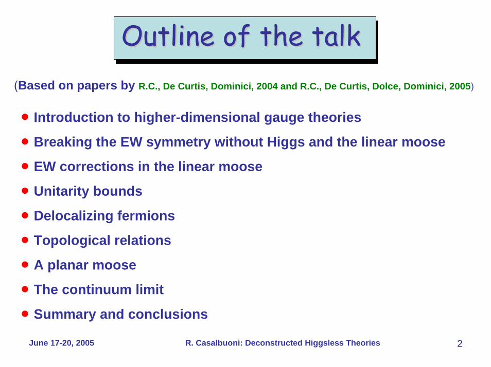
Outline of the talkOutline of the talk(Based on papers by R.C., De Curtis, Dominici, 2004 and R.C., De Curtis, Dolce, Dominici, 2005)

• Introduction to higher-dimensional gauge theories

• Breaking the EW symmetry without Higgs and the linear moose

• EW corrections in the linear moose

• Unitarity bounds

• Delocalizing fermions

• Topological relations

• A planar moose

• The continuum limit

• Summary and conclusions


Higher Dimensional Gauge TheoriesHigher Dimensional Gauge Theories

2 d 2 dP DM R M +=

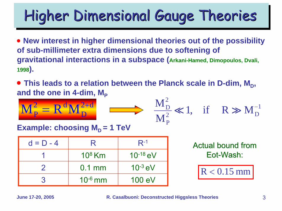
• New interest in higher dimensional theories out of the possibility of sub-millimeter extra dimensions due to softening of gravitational interactions in a subspace (Arkani-Hamed, Dimopoulos, Dvali, 1998).

• This leads to a relation between the Planck scale in D-dim, MD, and the one in 4-dim, MP

21D

D2P

M 1, if R MM

−

Example: choosing MD = 1 TeV

d = D - 4 R R-1

1 108 Km 10-18 eV2 0.1 mm 10-3 eV3 10-6 mm 100 eV

Actual bound from Actual bound from EotEot--Wash:Wash:

R 0.15 mm<


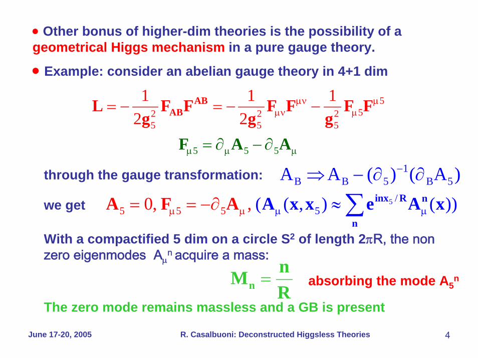
• Other bonus of higher-dim theories is the possibility of a geometrical Higgs mechanism in a pure gauge theory.

• Example: consider an abelian gauge theory in 4+1 dim

552 2 2

5

5

5

5 5

5

1 1 12 2

ABAB

F

L F F F F F Fg g

A Ag

µν µµν

µ µ µ

µ

= ∂

= −

− ∂

= − −

1B B 5 B 5A A ( ) ( A )−⇒ − ∂ ∂

55 5

/55 ( ( ,0, , ) ( ))inx R n

n

A x x eA AA F xµµ µµ= = −∂ ≈

through the gauge transformation:

we get ∑With a compactified 5 dim on a circle S2 of length 2πR, the non zero eigenmodes Aµ

n acquire a mass:

=nnMR

absorbing the mode A5n

The zero mode remains massless and a GB is present


• Massless modes can be eliminated compactifying on an orbifold, that is

25 5/ , :S Z Z x x→ −

• This allows to define fields as eigenstates of parity:

B 5 B 5A (x ,x ) A (x , x )µ µ= ± −

• Various possibilities, for instance by choosing:

BA odd no zero mode only massive gauge bosons in the spectrum

⇒ ⇒

Very nice geometrical structure through discretization of the extra-dim (Hill, Pokorski, Wang, 2001). One gets a deconstructed gauge theory


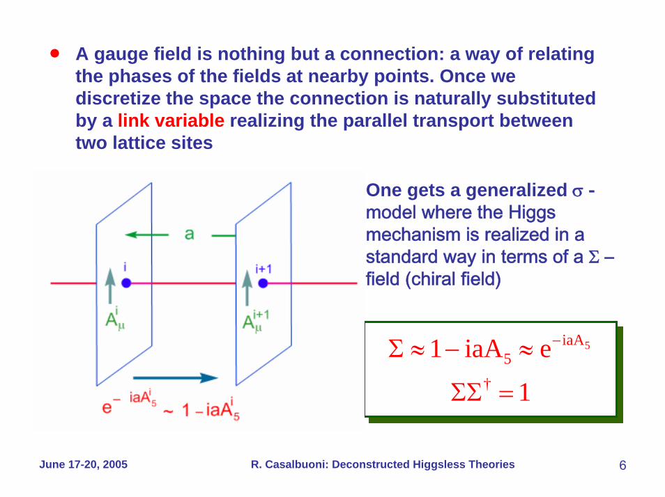
• A gauge field is nothing but a connection: a way of relating the phases of the fields at nearby points. Once we discretize the space the connection is naturally substituted by a link variable realizing the parallel transport between two lattice sites

5iaA5

†

1 iaA e

1

−Σ ≈ − ≈

ΣΣ =

One gets a generalized σ -model where the Higgs mechanism is realized in a standard way in terms of a Σ –field (chiral field)


i i

i 1 †i 5 i i 1 i iU G

i 1 i i 1i i i i 5

i i i i i5 5 5 5

1 iaA , U U

D iA i A iaF

F A A i[A ,A ]

−−∈

− −µ µ µ µ µ

µ µ µ µ

Σ = − Σ ⎯⎯⎯→ Σ

Σ = ∂ Σ − Σ + Σ =−

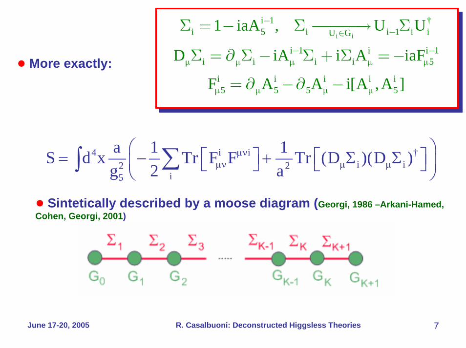
= ∂ −∂ −● More exactly:

4 i i †i i2 2

i5

a 1 1S d x Tr F F Tr (D )(D )g 2 a

µνµν µ µ

⎛ ⎞⎡ ⎤ ⎡ ⎤= − + Σ Σ⎜ ⎟⎣ ⎦ ⎣ ⎦⎝ ⎠∑∫

● Sintetically described by a moose diagram (Georgi, 1986 –Arkani-Hamed, Cohen, Georgi, 2001)


Breaking the EW Symmetry without Breaking the EW Symmetry without Higgs FieldsHiggs Fields

● Abstracting from the previous construction one can study more general moose geometries.

● General structure given by many copies of the gauge group G intertwined by link variables Σ.

● Condition to be satisfied in order to get a Higgsless SM before gauging the EW group is the presence of 3 GB and all the moose gauge fields massive.

● Simplest example: Gi = SU(2). Each Si describes three scalar fields. Therefore, in a connected moose diagram, any site (3 gauge fields) may absorb one link (3 GB’s) giving rise to a massive vector field. We need:

# of links = # of sites +1June 17-20, 2005 R. Casalbuoni: Deconstructed Higgsless Theories 8

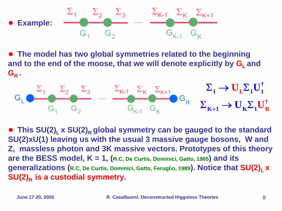
● Example:

● The model has two global symmetries related to the beginning and to the end of the moose, that we will denote explicitly by GL and GR .

†1 1 1

K 1 1

L

K†R

U

U

U

U+

Σ → Σ

Σ → Σ

● This SU(2)L x SU(2)R global symmetry can be gauged to the standard SU(2)xU(1) leaving us with the usual 3 massive gauge bosons, W and Z, massless photon and 3K massive vectors. Prototypes of this theory are the BESS model, K = 1, (R.C, De Curtis, Dominici, Gatto, 1985) and its generalizations (R.C, De Curtis, Dominici, Gatto, Feruglio, 1989). Notice that SU(2)L x SU(2)R is a custodial symmetry.


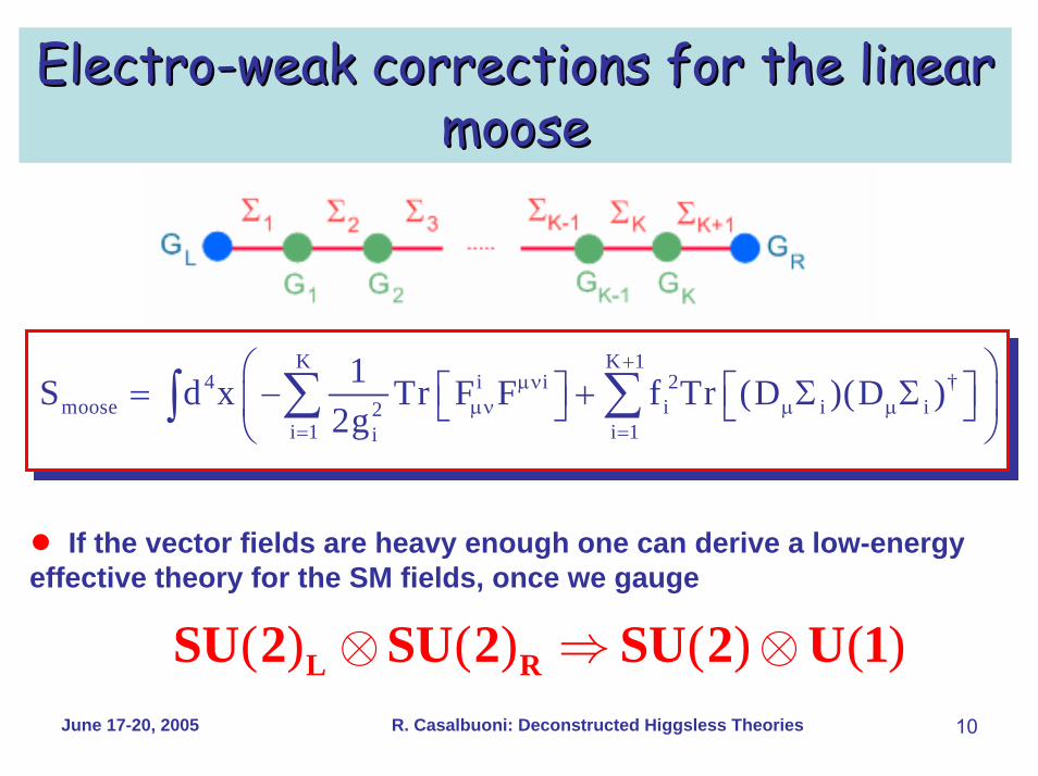
ElectroElectro--weak corrections for the linear weak corrections for the linear moosemoose

K K 14 i i 2 †

moose i i i2i 1 i 1i

1S d x Tr F F f Tr (D )(D )2g

+µν

µν µ µ= =

⎛ ⎞⎡ ⎤ ⎡ ⎤= − + Σ Σ⎜ ⎟⎣ ⎦ ⎣ ⎦

⎝ ⎠∑ ∑∫

● If the vector fields are heavy enough one can derive a low-energy effective theory for the SM fields, once we gauge

( ) ( ) ( ) ( )L RSU 2 SU 2 SU 2 U 1⊗ ⇒ ⊗June 17-20, 2005 R. Casalbuoni: Deconstructed Higgsless Theories 10

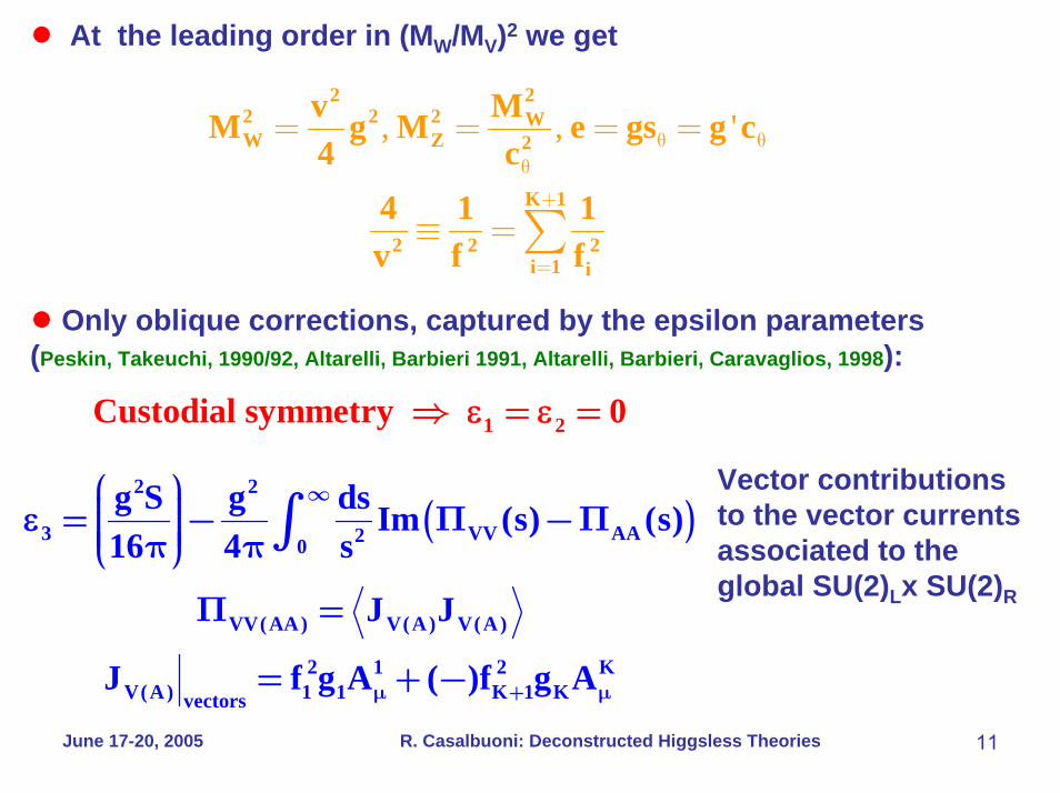
● At the leading order in (MW/MV)2 we get

, , '2 2

2 2 2 WW Z 2

K 1

2 2 2i 1 i

v MM g M e gs g c4 c

4 1 1v f f

θ θθ+

=

= = = =

≡ =∑● Only oblique corrections, captured by the epsilon parameters (Peskin, Takeuchi, 1990/92, Altarelli, Barbieri 1991, Altarelli, Barbieri, Caravaglios, 1998):

( )2 2

3 VV20

VV(AA) V(A) V(A)

2 1 2 KV(A) 1 1 K 1 Kvectors

1 2

g S g ds Im (

Custodial symmetry 0

s) (s)16 4 s

J J

J f g A ( )f g A

∞

µ + µ

⎛ ⎞⎜ ⎟= − Π −Π⎜ ⎟⎜ ⎟⎜ ⎟π π⎝ ⎠Π =

= + −

⇒ = =

∫

ε

ε

ε

AA

Vector contributions to the vector currents associated to the global SU(2)Lx SU(2)R


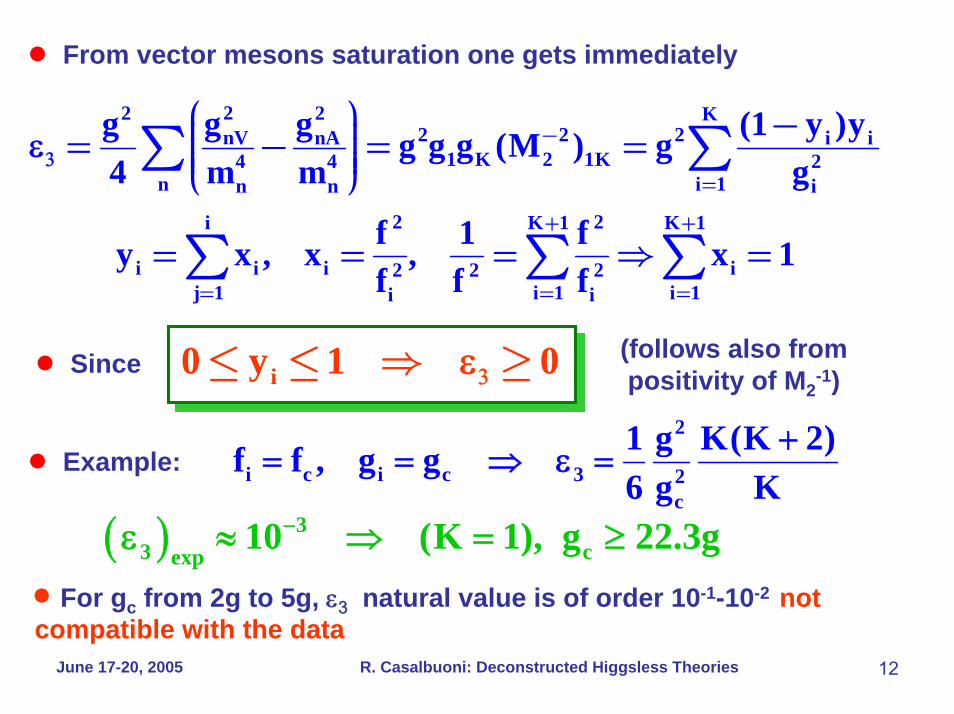
● From vector mesons saturation one gets immediately

22 2 K2 2 2nV nA i i

1 K 2 1K4 4 2n i 1n n i

2 2i K 1 K 1

i i i i2 2 2j 1 i 1 i 1i i

gg g (1 y )yg g g (M ) g4 m m g

f 1 fy x , x , x 1f f f

−

=

+ +

= = =

⎛ ⎞ −⎜ ⎟= − = =⎜ ⎟⎜ ⎟⎜ ⎟⎝ ⎠

= = = ⇒ =

∑ ∑

∑ ∑ ∑

3ε

i0 y 1 0≤ ≤ ⇒ ≥3ε (follows also from positivity of M2

-1)● Since

● Example: 2

i c i c 3 2c

1 g K(K 2)f f , g g6 g K

+= = ⇒ ε =

( ) 33 cexp

10 (K 1), g 22.3g−ε ≈ ⇒ = ≥

• For gc from 2g to 5g, ε3 natural value is of order 10-1-10-2 not compatible with the data


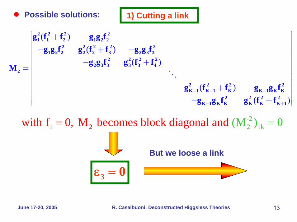
● Possible solutions: 1) Cutting a link

( )( )

( )

( )( )

2 2 2 21 1 2 1 2 2

2 2 2 2 21 2 2 2 2 3 2 3 3

2 2 2 22 3 3 3 3 4

2

2 2 2 2K 1 K 1 K K 1 K K

2 2 2 2K 1 K K K K K 1

g f f g g fg g f g f f g g f

g g f g f fM

g f f g g fg g f g f f

− − −

− +

⎡ ⎤+ −⎢ ⎥⎢ ⎥− + −⎢ ⎥⎢ ⎥− +⎢ ⎥= ⎢ ⎥⎢ ⎥⎢ ⎥+ −⎢ ⎥⎢ ⎥− +⎢ ⎥⎣ ⎦

-22 1ki 2with f 0, M becomes block diagonal and (M ) 0= =

But we loose a link

3 0ε =


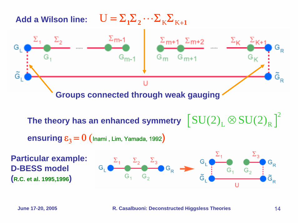
Add a Wilson line: K KU 1 2 1+= Σ Σ Σ Σ

Groups connected through weak gauging

The theory has an enhanced symmetry

ensuring ε3 = 0 (Inami , Lim, Yamada, 1992)[ ]2

L RSU(2) SU(2)⊗

Particular example: D-BESS model (R.C. et al. 1995,1996)



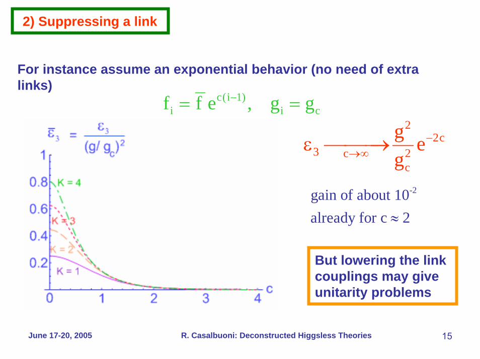
2) Suppressing a link

For instance assume an exponential behavior (no need of extra links)

c(i 1)i i cf f e , g g−= =

22c

3 2cc

g eg

−→∞ε ⎯⎯⎯→

-2gain of about 10 already for c 2≈

But lowering the link couplings may give unitarity problems

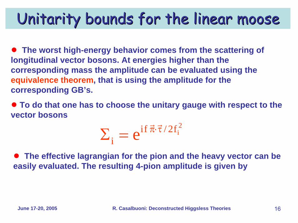
UnitarityUnitarity bounds for the linear moosebounds for the linear moose

● The worst high-energy behavior comes from the scattering of longitudinal vector bosons. At energies higher than the corresponding mass the amplitude can be evaluated using the equivalence theorem, that is using the amplitude for the corresponding GB’s.

● To do that one has to choose the unitary gauge with respect to the vector bosons

2iif / 2f

i e π⋅τΣ =● The effective lagrangian for the pion and the heavy vector can be easily evaluated. The resulting 4-pion amplitude is given by


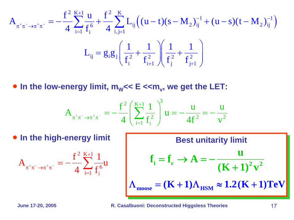
( )2 2K 1 K

1 1ij 2 ij 2 ij6

i 1 i, j 1i

ij i j 2 2 2 2i i 1 j j 1

f u fA L (u t)(s M ) (u s)(t M )4 f 4

1 1 1 1L g gf f f f

+ − + −

+− −

π π →π π= =

+ +

= − + − − + − −

⎛ ⎞⎛ ⎞= + +⎜ ⎟⎜ ⎟⎜ ⎟⎝ ⎠⎝ ⎠

∑ ∑

• In the low-energy limit, mW<< E <<mv, we get the LET:

2 K 1

6i 1 i

f 1A u4 f+ − + −

+

π π →π π=

= − ∑

• In the high-energy limit

32 K 1

2 2 2i 1 i

f 1 u uA u4 f 4f v+ − + −

+

π π →π π=

⎛ ⎞= − = − = −⎜ ⎟

⎝ ⎠∑

Best unitarity limit

i c 2 2uf f A

(K 1) v= → = −

+

moose HSM(K 1) 1.2(K 1)TeVΛ = + Λ ≈ +


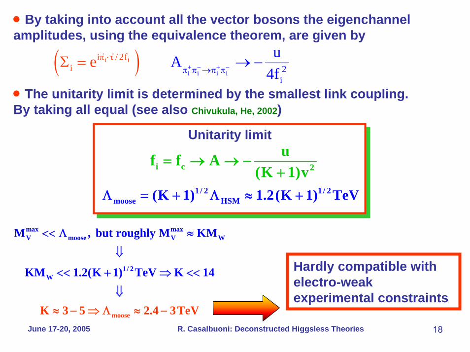
• By taking into account all the vector bosons the eigenchannelamplitudes, using the equivalence theorem, are given by

( )i i i

i i

ii

i f2

/ 2i

uA4f

e + − + −π ⋅τ

π π →π π→ −Σ =

• The unitarity limit is determined by the smallest link coupling. By taking all equal (see also Chivukula, He, 2002)

Unitarity limit

i c 2uf f A

(K 1)v= → → −

+1/ 2 1 / 2

moose HSM(K 1) 1.2(K 1) TeVΛ = + Λ ≈ +

max maxV moose

moos

W

2W

e

V

1/

M , but roughly M KM

KM 1.2(K 1) TeV

K 3 5 2.4 T

K 14

3 eV≈ − ⇒ Λ ≈

<< Λ ≈

⇓

<< + ⇒ <<

−⇓

Hardly compatible with electro-weak experimental constraints


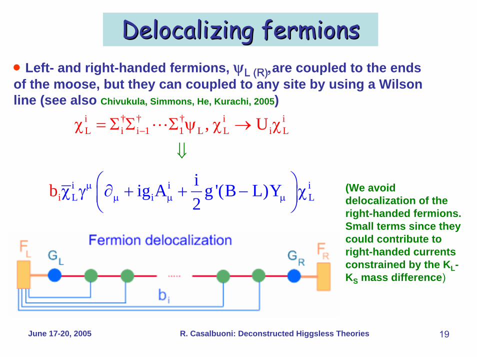
DelocalizingDelocalizing fermionsfermions• Left- and right-handed fermions, ψL (R),are coupled to the ends of the moose, but they can coupled to any site by using a Wilsonline (see also Chivukula, Simmons, He, Kurachi, 2005)

i

i † † † i iL i i 1 1 L L i

i iL i

L

iiig A g '(B L)Y

, U

b2

µµ µ µ

−χ = Σ Σ Σ

⎛ ⎞Lχ γ ∂ + + − χ⎜ ⎟

⎝

χ

⇓

⎠

ψ → χ

(We avoid delocalization of the right-handed fermions. Small terms since they could contribute to right-handed currents constrained by the KL-KS mass difference)


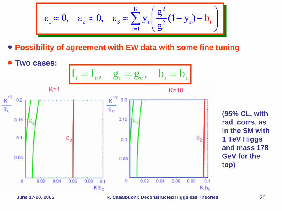
2K

1 2 i i2i

i3i 1

g0, 0, y (1 y ) bg=

⎛ ⎞ε ≈ ε ≈ ε ≈ − −⎜ ⎟

⎝ ⎠∑

• Possibility of agreement with EW data with some fine tuning

• Two cases:


i c i c i cf f , g g , b b= = =

(95% CL, with rad. corrs. as in the SM with 1 TeV Higgs and mass 178 GeV for the top)


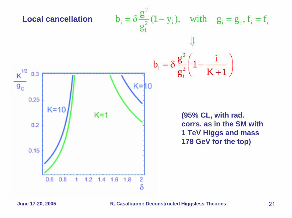
2

i i

2

i

i c

2

i c2i

i

gb (1 y ), with g g , f

g ibK

g

1g 1

f=

⎛ ⎞= δ −⎜ ⎟+

=

⇓

⎝

− =

⎠

δLocal cancellation

(95% CL, with rad. corrs. as in the SM with 1 TeV Higgs and mass 178 GeV for the top)

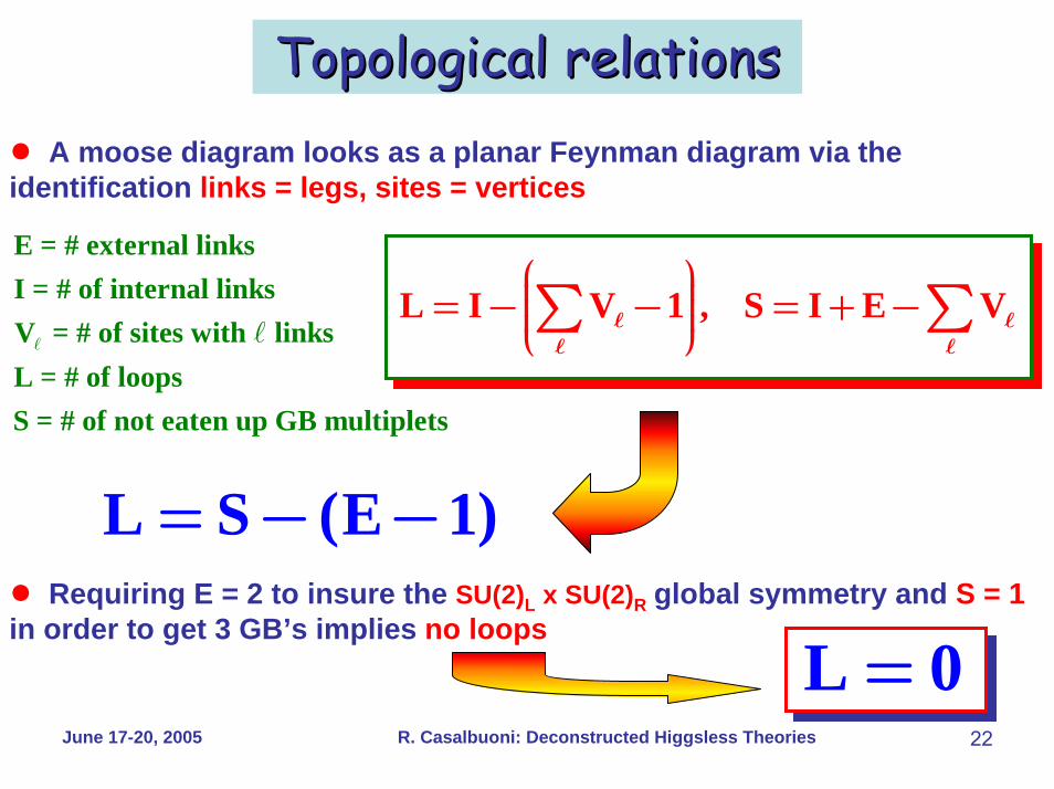
Topological relationsTopological relations● A moose diagram looks as a planar Feynman diagram via the identification links = legs, sites = vertices

E = # external linksI = # of internal linksV = # of sites with linksL = # of loopsS = # of not eaten up GB multiplets

L I V 1 , S I E V⎛ ⎞⎜ ⎟= − − = + −⎜ ⎟⎜ ⎟⎝ ⎠∑ ∑

L S (E 1)= − −● Requiring E = 2 to insure the SU(2)L x SU(2)R global symmetry and S = 1 in order to get 3 GB’s implies no loops

L 0=June 17-20, 2005 R. Casalbuoni: Deconstructed Higgsless Theories 22

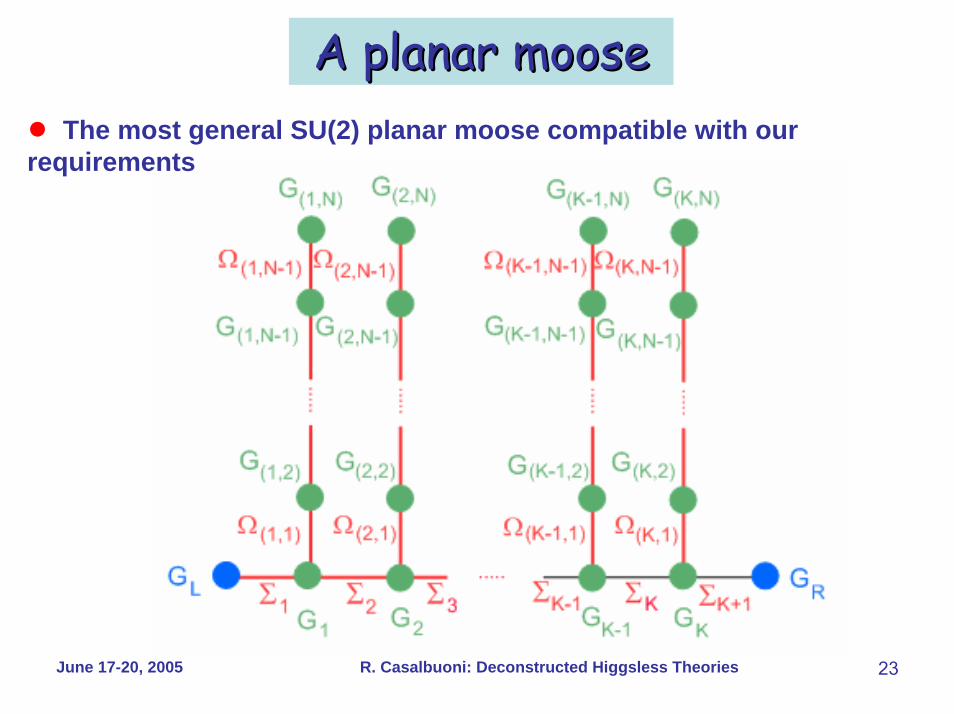
A planar mooseA planar moose● The most general SU(2) planar moose compatible with our requirements


● These two moose are equivalent through the substitution:N

2 2j 11 (1j)

1 1g g=

→ ∑N

2 2j 1i (ij)

1 1g g=

→ ∑● In general the planar moose is equivalent to a linear one with an analogous substitution


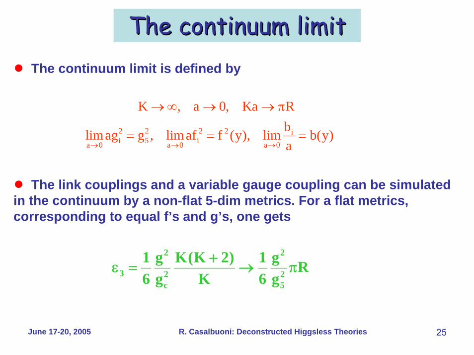
The continuum limitThe continuum limit● The continuum limit is defined by

2 2 2 2 ii 5 ia 0 a 0 a 0

K , a 0, Ka Rblimag g , limaf f (y), lim b(y)a→ → →

→ ∞ → → π

= = =

● The link couplings and a variable gauge coupling can be simulated in the continuum by a non-flat 5-dim metrics. For a flat metrics, corresponding to equal f’s and g’s, one gets

2 2

3 2 2c 5

1 g K(K 2) 1 g R6 g K 6 g

+ε = → π


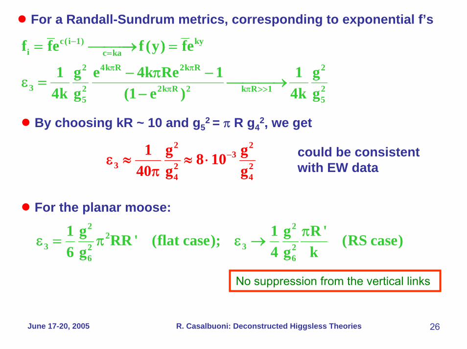
● For a Randall-Sundrum metrics, corresponding to exponential f’s

c(i 1) kyi c ka

2 4k R 2k R 2

3 2 2k R 2 2k R 15 5

f fe f (y) fe

1 g e 4k Re 1 1 g4k g (1 e ) 4k g

−=

π π

π π >>

= ⎯⎯⎯→ =

− π −ε = ⎯⎯⎯→

−

● By choosing kR ~ 10 and g52 = π R g4

2, we get

could be consistent with EW data

2 23

3 2 24 4

1 g g8 1040 g g

−ε ≈ ≈ ⋅π

● For the planar moose:

2 2

23 32 2

6 6

1 g 1 g R'RR' (flat case); (RS case)6 g 4 g k

πε = π ε →

No suppression from the vertical links


Summary and ConclusionsSummary and Conclusions

● Higher dimensional gauge theories naturally suggest the possibility of Higgsless theories.

● Study in 4-dim through discrete extra-dim leads to moose theories.

● Simplest case: the linear moose.

● Difficulties with EW corrections similar to TC models.

● EW corrections and raising the unitarity bounds push in different directions.

● Possibility of easing the theory delocalizing the fermions and using some fine tuning.


Deconstructed Higgsless Models - Florence Theory...

Documents

Transcript of Deconstructed Higgsless Models - Florence Theory...