DECOMPOSITION OF GENDER WAGE GAP IN POLAND USING … · 172 J. M. Landmesser: Decomposition of...

STATISTICS IN TRANSITION new series, September 2019

171

STATISTICS IN TRANSITION new series, September 2019 Vol. 20, No. 3, pp. 171–186, DOI 10.21307/stattrans-2019-030 Submitted – 10.01.2019; Paper ready for publication – 11.04.2019

DECOMPOSITION OF GENDER WAGE GAP IN POLAND USING COUNTERFACTUAL DISTRIBUTION WITH SAMPLE

SELECTION

Joanna Małgorzata Landmesser1

ABSTRACT

In the paper, we compare income distributions in Poland taking into account gender differences. The gender pay gap can only be partially explained by differences in men’s and women’s characteristics. The unexplained part of the gap is usually attributed to the wage discrimination. The objective of this study is to extend the Oaxaca-Blinder decomposition procedure to different quantile points along the income distribution. We use the RIF-regression method to describe differences between the incomes of men and women along the two distributions and to evaluate the strength of the influence of personal characteristics on the various parts of the income distributions. As the sample selection is a serious issue for the study, therefore our decomposition approach will be adjusted for sample selection problems. The results suggest not only differences in the income gap along the income distribution (in particular sticky floor and glass ceiling), but also differences in the contribution of selection effects to the pay gap at different quantiles. The analysis is based on data from the EU-SILC data for Poland in 2014.

Key words: gender wage gap, sample selection, decomposition of income

inequalities.

1. Introduction

Gender differences in pay are a well-known phenomenon of labour markets. Also, researchers investigating the wage gap in Poland have found significant gender differences. Goraus, Tyrowicz and van der Velde (2017) report that the raw wage gap is around 10% and the adjusted pay gap estimates oscillate between 14% and 24% depending on the method of calculation. All studies indicate that women are paid only a part of what men with similar demographic characteristic, family situations, working hours, educational levels and work experience are paid. Goraus and Tyrowicz (2014) studied the gender wage gap in Poland using the Labour Force Survey data covering the time span of 1995–2012. The raw gap was highest in the first and last five years of the analyzed

1 Warsaw University of Life Sciences – SGGW. E-mail: [email protected].

ORCID ID: http://orcid.org/0000-0001-7286-8536.

mailto:[email protected]

172 J. M. Landmesser: Decomposition of gender…

period and amounted to around 15% of average females’ wages. In the year 1999 the gap started decreasing and reached the level of around 2% in the years 2003 and 2004. Then the gap was increasing until it reached its previous level. The lowest levels of wage gap were observed after economic downturn in Poland. The adjusted gender wage gap was twice as high as the raw gender wage gap. The authors suggested that the adjusted gender wage gap has cyclical properties and it conforms to the bahaviour of unit labour costs - the more lax the labour market conditions, the higher the chances for women to be less unequally compensated.

According to the annual Global Gender Gap Report from the World Economic Forum (2018) women around the world earn about 20-30 percent less on average than their male counterparts. The inequalities between the sexes had closed by only a small amount in the past years. The largest gaps exist in politics, healthcare and education. A meta-analysis by Weichselbaumer and Winter-Ebmer (2005) of more than 260 published pay gap studies for over 60 countries found that, from the 1960s to the 1990s, raw wage differentials worldwide fell substantially from around 65% to 30%. The bulk of this decline was due to better labour market endowments of women (i.e. better education, training, and work attachment). In the period from 2010 to 2015, the gap decreased in only 10 of the 30 European countries (World Bank calculations using EU-SILC surveys for 30 countries in Europe). The most notable decreases were in Estonia, the Slovak Republic, and Switzerland. For others, the gap increased, particularly in Poland, Bulgaria, Lithuania, and France.

Numerous foreign publications show that such a factor as self-selection into the labour force is also crucial for the gender pay gap (e.g. Albrecht, van Vuuren and Vroman, 2009; Töpfer, 2017). If all women participated in the labour force, the observed gap would have a different size. Previous researchers in Poland focused on decomposing the gender pay gap at the means of the wage distribution using a procedure developed by Oaxaca (1973) and Blinder (1973). Using this method the gender wage gap could only be partially explained by differences in men’s and women’s characteristics (e.g. Słoczyński (2012), Śliwicki and Ryczkowski (2014)). Later, attention shifted to investigating the degree to which gender pay gaps might vary across the wage distribution (Rokicka and Ruzik (2010), Landmesser, Karpio and Łukasiewicz (2015), Magda, Tyrowicz and van der Velde(2015), Landmesser (2016)). Various techniques for the decomposition of differences in income distributions were considered but they lack women self-selection.

The objective of this study is to extend the Oaxaca-Blinder decomposition procedure to different quantile points along the income distribution. The employment rates in Poland differ by gender and the sample selection is a serious issue for the study. Therefore, our decomposition approach will be adjusted for sample selection problems.

We focus our attention on people's decisions regarding full-time or part-time employment, which seem to be non-random. According the Polish Central Statistical Office (2016), the share of part-time employees among the total working population for men is equal to 4.7 and for women to 10.7. Part-time employment in Poland is therefore more concentrated among women. The main reasons given by people for part-time work are: a person prefers this kind of work


173

(the answer given by 46.2% of men and 42.3% of women who worked part-time), a person is unable to find full-time work (25.1% of men and 27.3% of women), care for children and other people, other personal or family reasons (only 3.3% of men and 13.1% of women), education, illness or disability (Central Statistical Office, 2016). However, our empirical investigation is based on data from the European Union Statistics on Income and Living Conditions project for Poland, which made it impossible to take into account all the factors mentioned above.

To decompose the differences between two distributions one uses the so-called counterfactual distribution, which is a mixture of a conditional distribution of the dependent variable and a distribution of the explanatory variables. Such a counterfactual distribution can be constructed in various ways (DiNardo, Fortin and Lemieux (1996), Donald, Green and Paarsch (2000), Machado and Mata (2005), Fortin, Lemieux and Firpo (2010)). We will examine the differences in the entire range of income values by the use of the RIF-regression method (recentered influence function) (Firpo, Fortin and Lemieux (2009)) corrected in a way that allows us to include non-random selection into the sample. It will also be found how the men’s and women’s characteristics (the explanatory variables in estimated models) influence various ranges of income distributions.

2. Methods of the analysis

Let Yg denote the outcome variable in group g (e.g. the personal income in men’s group, g=M, or in women’s group, g=W) and Xg the vector of individual characteristics of the person in group g (e.g. age, education level, number of years spent in paid work). The expected value of y conditionally on X is a linear

function WMgvXy gggg ,, , where g are the returns to the

characteristics. The Oaxaca-Blinder decomposition for the average income inequality between two groups at the aggregate level can be expressed as

dunexplaineexplainedˆ

)ˆˆ(

ˆ

ˆ)(ˆˆˆ

WMWMWMWWMMWM XXXXXYY . (1)

The first component, on the right side of the equation, gives the effect of characteristics and expresses the difference of the potentials of people in two groups (the so-called explained effect). The second term called the unexplained effect, is the result of differences in the returns to observables. This is the result of differences in the estimated parameters, and so in the “prices” of individual characteristics of group representatives. It can be interpreted as the labour market discrimination. Also, the detailed decomposition may be calculated. A drawback of the approach is that it focuses only on average effects, which may lead to a misleading assessment if the effects of covariates vary across the wage distribution.

In our study people participate in the labour market full-time or part-time. Those who work full-time have higher incomes and those who work part-time have lower incomes. The decision on working time is subjective and non-random. Therefore, our decomposition approach will be adjusted for sample selection.


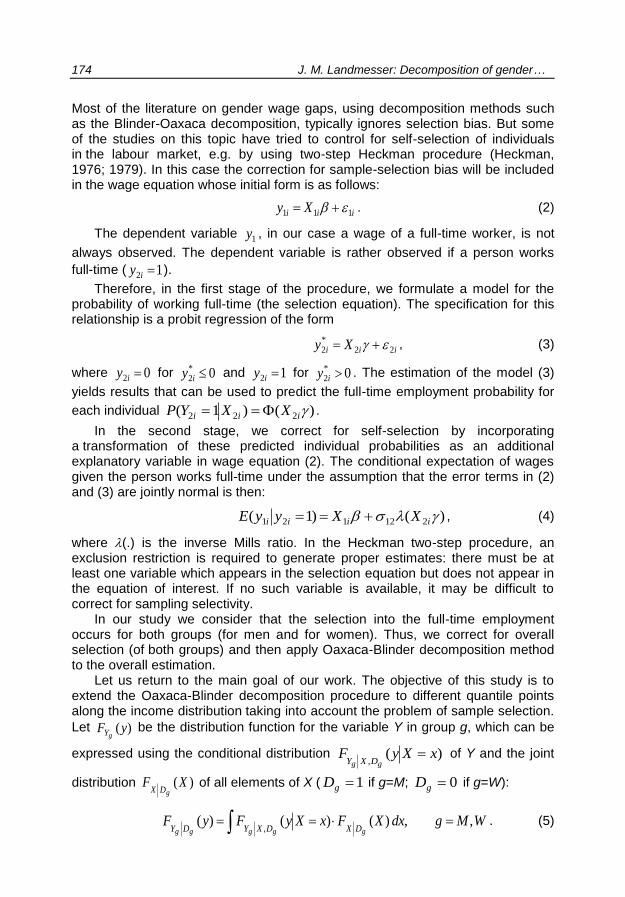
Most of the literature on gender wage gaps, using decomposition methods such as the Blinder-Oaxaca decomposition, typically ignores selection bias. But some of the studies on this topic have tried to control for self-selection of individuals in the labour market, e.g. by using two-step Heckman procedure (Heckman, 1976; 1979). In this case the correction for sample-selection bias will be included in the wage equation whose initial form is as follows:

iii Xy 111 . (2)

The dependent variable 1y , in our case a wage of a full-time worker, is not

always observed. The dependent variable is rather observed if a person works

full-time ( 12 iy ).

Therefore, in the first stage of the procedure, we formulate a model for the probability of working full-time (the selection equation). The specification for this relationship is a probit regression of the form

iii Xy 22*2 , (3)

where 02 iy for 0*2 iy and 12 iy for 0*

2 iy . The estimation of the model (3)

yields results that can be used to predict the full-time employment probability for

each individual )()1( 222 iii XXYP .

In the second stage, we correct for self-selection by incorporating a transformation of these predicted individual probabilities as an additional explanatory variable in wage equation (2). The conditional expectation of wages given the person works full-time under the assumption that the error terms in (2) and (3) are jointly normal is then:

)()1( 212121 iiii XXyyE , (4)

where (.) is the inverse Mills ratio. In the Heckman two-step procedure, an exclusion restriction is required to generate proper estimates: there must be at least one variable which appears in the selection equation but does not appear in the equation of interest. If no such variable is available, it may be difficult to correct for sampling selectivity.

In our study we consider that the selection into the full-time employment occurs for both groups (for men and for women). Thus, we correct for overall selection (of both groups) and then apply Oaxaca-Blinder decomposition method to the overall estimation.

Let us return to the main goal of our work. The objective of this study is to extend the Oaxaca-Blinder decomposition procedure to different quantile points along the income distribution taking into account the problem of sample selection.

Let )(yFgY

be the distribution function for the variable Y in group g, which can be

expressed using the conditional distribution )(,

xXyFgg DXY

of Y and the joint

distribution )(XFgDX

of all elements of X ( 1gD if g=M; 0gD if g=W):

WMgdxXFxXyFyFggggg DXDXYDY

,,)()()(,

. (5)

https://en.wikipedia.org/wiki/Probit


175

We can extend the mean decomposition analysis to the case of differences between the two distributions using the counterfactual distribution

)()()( XdFXyFyFMWW

CW

XXYY (distribution of incomes that would prevail for

people in group W if they had the distribution of characteristics of group M):

.

ˆ

)]()([

Δ̂

)]()([)()(

effect)on(compositiexplained

effect)(structure

μdunexplaine

yFyFyFyFyFyFWC

WC

WMWM YYYYYY (6)

The counterfactual distribution can be constructed using the RIF-regression method by Firpo, Fortin and Lemieux (2009). This method is similar to a linear regression, except that the variable Y is replaced by the recentered influence function of the statistic of interest. The recentered influence function is defined as:

)(

}{),(),(

Qf

QyQQyIFQQyRIF

Y

, (7)

where ),( QyIF is the influence function corresponding to an income y for the

quantile Q of the distribution FY, and }{ Qy is the indicator variable for

whether the income y is smaller or equal to the quantile Q . Firpo, Fortin and

Lemieux (2009) model the conditional expectation of ),( QyRIF as a linear

function of the explanatory variables XXQyRIFE )],([ , where the

parameters can be estimated by

OLS ( WMgQyRIFXXXgi

gigTi

gi

iTig ,,),()(ˆ

,,1

,

). In the approach,

we first compute the sample quantile Q̂ and estimate the density )ˆ(ˆQfY using

kernel methods. Then, we estimate the linear probability model for the proportion

of people with income less than Q̂ , calculate RIF of each observation and run

regressions of RIF on the vector X. The aggregated and detailed decomposition for any unconditional quantile is then:

k

j

jWjMjMjWjWjM

WMMWWM

XXX

XXX

1

,,,

,,,

))ˆˆ(ˆ)((

)ˆˆ(ˆ)(ˆ

(8)

Now, following Buchinsky (1998) we propose the RIF-model corrected for

selectivity bias at the th quantile:

222211 )()(),( XXXQyRIF , (9)

where (.) is the standard inverse Mills ratio (compare with other approaches in Albrecht, van Vuuren and Vroman (2009), Töpfer (2017)). By that means, we will examine the differences in the entire range of income values by the use of the


RIF-regression method corrected in a way that allows us to include non-random selection into the sample. It would be also possible to compare the income distributions of men and women by building a model for people working only full-time, although it seems that this would be an oversimplification of the problem.

3. Data basis

The empirical data used were collected within the European Union Statistics on Income and Living Conditions project for Poland in 2014 (research proposal 234/2016-EU-SILC). The sample consists of 5,181 men and 4,734 women. Each person is described by the following characteristics: age (in years), educlevel

(education level, 1 primary, . . ., 5 tertiary), married (marital status,

1 married, 0 unmarried), yearswork (number of years spent in paid work),

permanent (type of contract, 1 permanent job/work contract of unlimited

duration, 0 temporary contract of limited duration), parttime (1 person working

part-time, 0 person working full-time), manager (managerial position,

1 supervisory, 0 non-supervisory). The sample features are presented in Table 1 and Table 2.

Table 1. The selected sample features

Characteristic Men Women Characteristic Men Women

No. of obs. 5,181 4,734 Average age 42.07 42.36

Average income 7,165.94 5,900.21 Average yearswork 20.09 18.46

educlevel

= 1 4.91% 3.89%

= 2 1.45% 0.55% married = 1 71.53% 69.60%

= 3 68.57% 47.32% permanent = 1 70.60% 71.63%

= 4 2.55% 7.91% parttime = 1 4.31% 10.09%

= 5 22.52% 40.32% manager = 1 18.68% 15.74%

Source: Own calculations.

Table 2. The number of observations and the average annual net employee incomes of men and women

Men Women

full-time part-time full-time part-time

Number of observations 4957 224 4257 477

The average annual net employee incomes in thousands of Euros

7,326.65 3,562.56 6,206.51 3,147.30

The average logarithm of the annual income

8.707 7.817 8.564 7.765


Since there was no information in the EU-SILC database on the hourly

income, in our analysis the annual net employee (cash or near cash) incomes of men were compared with those obtained by women. Employee income is defined as the total remuneration payable by an employer to an employee in return for


177

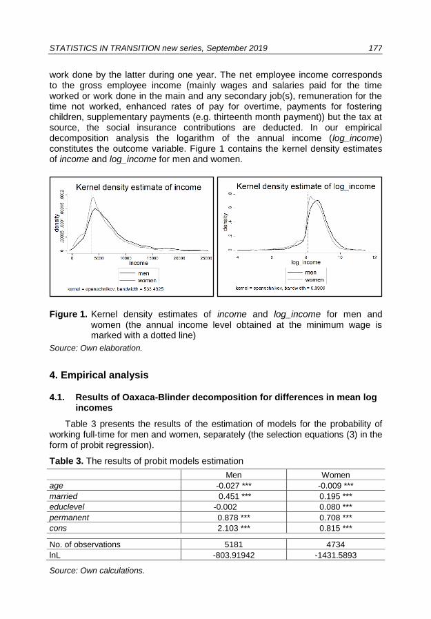
work done by the latter during one year. The net employee income corresponds to the gross employee income (mainly wages and salaries paid for the time worked or work done in the main and any secondary job(s), remuneration for the time not worked, enhanced rates of pay for overtime, payments for fostering children, supplementary payments (e.g. thirteenth month payment)) but the tax at source, the social insurance contributions are deducted. In our empirical decomposition analysis the logarithm of the annual income (log_income) constitutes the outcome variable. Figure 1 contains the kernel density estimates of income and log_income for men and women.

Figure 1. Kernel density estimates of income and log_income for men and women (the annual income level obtained at the minimum wage is marked with a dotted line)

Source: Own elaboration.

4. Empirical analysis

4.1. Results of Oaxaca-Blinder decomposition for differences in mean log incomes

Table 3 presents the results of the estimation of models for the probability of working full-time for men and women, separately (the selection equations (3) in the form of probit regression).

Table 3. The results of probit models estimation

Men Women

age -0.027 *** -0.009 ***

married 0.451 *** 0.195 ***

educlevel -0.002 0.080 ***

permanent 0.878 *** 0.708 ***

cons 2.103 *** 0.815 ***

No. of observations 5181 4734

lnL -803.91942 -1431.5893


https://en.wikipedia.org/wiki/Probit


Then, after estimating the wage equations, we compare the results of aggregate and detailed Oaxaca-Blinder decomposition of inequalities between men’s and women’s log incomes without and with selection adjustment (Table 4). For this purpose, we have used the following code prepared in Stata:

probit fulltime age married educlevel permanent if men==0

predict Xbw if men==0, xb

gen millsw = . if men==0

replace millsw = normalden(Xbw) / normal(Xbw) if men==0 & fulltime==1

replace millsw = -normalden(Xbw) / normal(-Xbw) if men==0 & fulltime==0

probit fulltime age married educlevel permanent if men==1

predict Xbm if men==1, xb

gen millsm = . if men==1

replace millsm = normalden(Xbm) / normal(Xbm) if men==1 & fulltime==1

replace millsm = -normalden(Xbm) / normal(-Xbm) if men==1 & fulltime==0

gen mills = .

replace mills = millsw if men==0

replace mills = millsm if men==1

oaxaca2 logincome educlevel yearswork manager, by(men) weight(1)

oaxaca2 logincome educlevel yearswork manager mills, by(men) weight(1)

The variables which appear in the selection equation but do not appear in the income equation are age, married, permanent. Hence, the identification requirement for the model has been satisfied. Only the variable kids would be a better instrument, but it does not appear in the database used.

Table 4. The Oaxaca-Blinder decomposition of the average log income differences without and with selection adjustment

Mean log income men 8.670

Mean log income women 8.484

Raw differential 0.186

without selection with selection

Aggregate decomposition

Explained component -0.071 -0.072

Unexplained component 0.257 0.258

% explained 38.13% 38.71%

% unexplained -138.13% -138.71%

Detailed decomposition

explained unexplained explained unexplained

educlevel -0.108 *** -0.166 *** -0,109 *** -0,166 ***

yearswork 0.029 *** -0.143 *** 0,028 *** -0,136 ***

manager 0.009 *** 0.018 *** 0,008 *** 0,020 ***

mills

0,000 0,000

cons

0.548 ***

0,540 ***

Total -0.071 *** 0.257 *** -0,072 *** 0,258 ***

Source: Own elaboration using the Stata command ‘oaxaca2’.


179

The mean predicted log income for men equals 8.670 (annual net income = 5,825.50 Euro), and for women equals 8.484 (annual net income = 4,831.92 Euro) (see Table 4). There is a positive difference between the mean values of log incomes for men or women (the mean log income differential is 0.186). The difference between the mean log income values was decomposed into two components: the first one explaining the contribution of the attributes differences (the explained part) and the second one explaining the contribution of the different values of models coefficients (the unexplained part). The explained is very low and negative, but the unexplained effect is huge and positive, which means that the inequalities examined should be assigned, in the majority, to the coefficients of estimated models (rather than to the differentiation of individual characteristics). Unfortunately, the selection effect is statistically insignificant.

The detailed decomposition, which was also carried out, made it possible to isolate the factors explaining the inequality observed to a different extent. The strong effect of different education levels of men and women can be noticed. The negative value of the adequate component means that the difference of the average log incomes between men and women is mostly reduced by the women’s higher education levels. On the other hand, the values of manager attribute possessed by men and women increase the inequality in the average log incomes. A different “evaluation” of personal characteristics (the unexplained component) allow the conclusion that women are discriminated against men (but not because of the education levels and years of work).

4.2. Results of the aggregate decomposition along the income distribution using the residual imputation approach

Since the Oaxaca-Blinder technique focuses only on average effects, next we present the decomposition of inequalities along the distribution of log incomes for men and women using the RIF-approach without and with selection adjustment. The results of this decomposition are shown in Table 5, where the inequalities are expressed in terms of percentiles. The symbols p10, …, p90 stand for 10th, …, 90th percentile (e.g. the 10th percentile is the log income value below which 10% of the observations may be found). For each of the nine percentiles the total differences between the values of log incomes for men and women were computed. Then these differences are expressed as the sum of the explained and unexplained components.

Table 5. The results of the decomposition using the RIF-regression approach

Percentile total difference without selection with selection


p10 0.287 -0.036 0.322 0.004 0.283

p20 0.094 -0.030 0.124 0.014 0.081

p30 0.152 -0.045 0.198 -0.001 0.153

p40 0.147 -0.054 0.201 -0.002 0.149

p50 0.140 -0.060 0.200 -0.010 0.151

p60 0.141 -0.062 0.203 -0.019 0.160

p70 0.135 -0.064 0.199 -0.025 0.160

p80 0.163 -0.078 0.242 -0.043 0.207

p90 0.216 -0.086 0.302 -0.065 0.282

Source: Own elaboration using the Stata command ‘rifreg’.


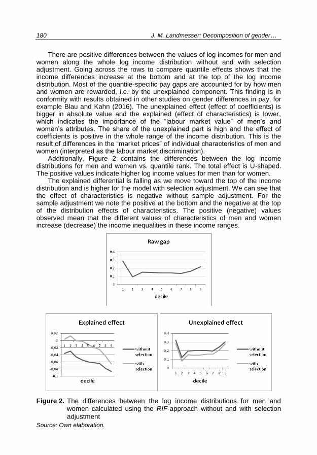
There are positive differences between the values of log incomes for men and women along the whole log income distribution without and with selection adjustment. Going across the rows to compare quantile effects shows that the income differences increase at the bottom and at the top of the log income distribution. Most of the quantile-specific pay gaps are accounted for by how men and women are rewarded, i.e. by the unexplained component. This finding is in conformity with results obtained in other studies on gender differences in pay, for example Blau and Kahn (2016). The unexplained effect (effect of coefficients) is bigger in absolute value and the explained (effect of characteristics) is lower, which indicates the importance of the “labour market value” of men’s and women’s attributes. The share of the unexplained part is high and the effect of coefficients is positive in the whole range of the income distribution. This is the result of differences in the “market prices” of individual characteristics of men and women (interpreted as the labour market discrimination).

Additionally, Figure 2 contains the differences between the log income distributions for men and women vs. quantile rank. The total effect is U-shaped. The positive values indicate higher log income values for men than for women.

The explained differential is falling as we move toward the top of the income distribution and is higher for the model with selection adjustment. We can see that the effect of characteristics is negative without sample adjustment. For the sample adjustment we note the positive at the bottom and the negative at the top of the distribution effects of characteristics. The positive (negative) values observed mean that the different values of characteristics of men and women increase (decrease) the income inequalities in these income ranges.

Figure 2. The differences between the log income distributions for men and

women calculated using the RIF-approach without and with selection

adjustment



181

The lower values of the unexplained effect after taking into account the selection imply that without selection correction we overestimate the part attributed to gender-wage discrimination. All in all, the selection component is one of the most important components explaining gender differences in pay along the income distribution.

4.3. Results of the detailed decomposition using the RIF-regression approach

The RIF-regression method enables us also to extend our analysis to the case of the detailed decomposition. Table 6 shows one of many results obtained of the detailed decomposition of inequalities along log income distributions.

Table 6. The example results of the RIF-regression approach – for 70th percentile only

Total gap 0.135 *** 0.135 ***

without selection with selection


educlevel -0.091 *** -0.304 *** -0.089 *** -0.276 ***

yearswork 0.013 *** -0.141 *** 0.014 *** -0.122 ***

manager 0.014 *** 0.021 *** 0.013 *** 0.021 ***

mills

0.000 0.000

mills^2

0.038 *** -0.015

cons

0.624 ***

0.552 ***

Total -0.064 *** 0.199 *** -0.025 ** 0.160 ***

Source: Own elaboration using the Stata command ‘rifreg’.

These are only the results for 70th percentile of log income distributions. In all, nine detailed decompositions for each decile were carried out (the results for the remaining eight deciles and the bootstrap errors are not presented here due to lack of space).

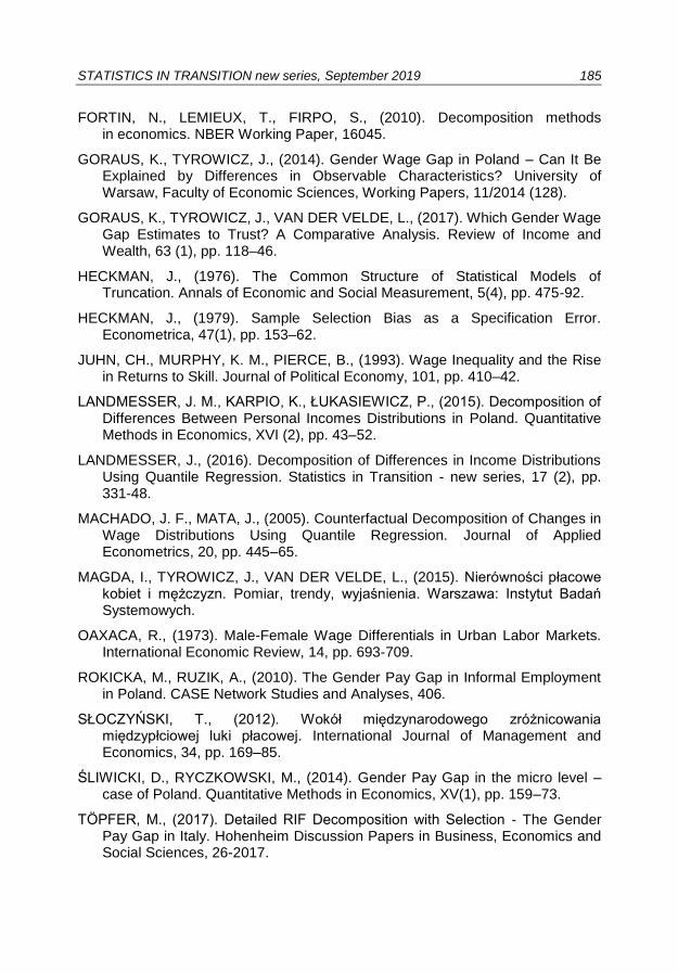
For better understanding of the results obtained and in order to formulate general conclusions, in Figure 3 we draw the values of explained component for each variable and for each decile group (vs. quantile rank), for the log income inequalities observed between men and women. The ordinate axes present the

values ,ˆ)( jMjWjM XX (detailed explained effects).

The educlevel has the greatest reduced influence on the differences between the log income distributions for men and women. It means that on average higher level of education among women decreases the income inequalities, especially as we move toward the top of the income distribution. For the variable yearswork we observe the influence which enlarges log income differences but increasingly less as we move toward the top of the income distribution. The variable manager also


enlarges log income differences but more and more as we move toward the top of the distribution.

With the increase in incomes the importance of the explained selection effect (which is unfavourable for women because of its positive share in the gap) decreases. According to Figure 2, after taking the selection into account, the explained effect is initially positive, which means that the characteristics of the poorest people enlarge the gap. Then, the explained effect is negative, meaning that the characteristics of the richest reduce the gap. Thus, with the increase in incomes, the importance of the people’s characteristics increases in the sense that they reduce the gap effect for women.

Figure 3. The results of the RIF-regression approach for the detailed income inequalities decomposition without and with selection adjustment – the explained effects


5. Conclusions

In recent times, particular attention of European politicians has focused on the gender pay gap. There is no clear idea of whether to use the raw or the adjusted gender pay gap for the analysis. Some experts claim that the explained part of the gap may reflect discriminatory social norms or discrimination related to education and occupational choice. Therefore, the use of the unadjusted gap but in tandem


183

with the employment rates among women should be preferred to analyze the problem.

According to European Union politicians, active policies to close wage gaps are required. The European Commission recommendations point to several possible directions, from pay transparency to improving legal frameworks. The progress on gender pay equality depends on developing specific gender equality policies. However, postulated policies for flexible working can lead to the widening of the gender pay gap if they result, e.g. in an increase in part-time work. A good example is Sweden, which has been at the forefront of gender equity efforts for decades. The universal child care, the protection of mothers’ right to work or tough employment laws on pay equity were practiced there. However, the last OECD report reveals the persistence of significant gender earnings gaps in Sweden. The way to close this gap would be if women worked longer hours or if men worked fewer hours. But the majority of Swedish women prefer to work part-time and less than men for a variety of reasons and the gender pay gap is largely a result of the freely-made women’s choices. Therefore, maybe we should not consider gaps that arise in these ways to be problems in need of fixing.

Like other researchers, we expected that such a factor as self-selection into the labour force may affect the size of the gender pay gap. Therefore, the goal of this paper was to present the decomposition of inequalities between log incomes for men and women in Poland, taking into account sample selection issues. We started with the decomposition of the average values for log incomes by using the Oaxaca-Blinder method. We found that there is a positive difference between the mean income values for men and women. The unexplained effect was big, but the explained was low. The decomposition showed the influence of the men’s and women’s attributes on the average log income differences. The selection effect was statistically insignificant.

Then, we decomposed the inequalities between log incomes along the whole distribution using the RIF-regression method. The total effect was U-shaped. The explained effect was low again. We claim that Polish women experience both a 'glass ceiling effect' and also a 'sticky floor effect' because gender differences primarily affect women at the top and the bottom of the distribution.

In our research the method of RIF-regression provided a way of showing the detailed decomposition of income inequalities and helped to exhibit the influence of the attributes on the whole log income distribution. The variable educlevel exerted the greatest reduced influence on the differences between the income distributions for men and women. Higher average levels of education among women decreased the income inequalities. The importance of educlevel characteristic increased with income. For the variable yearswork (years spent in paid work) we noted the influence which increases income differences but the effect was weaker as the income grew. A woman with the same number of years of work as a man will be more discriminated in the group of low-income people. We also observed strong impact of managerial position in higher quantiles of income distribution, which indicates a shift of big incomes towards men. Being a manager puts men in a more privileged position, especially when it concerns highly paid executive positions.

Also, self-selection into the labour force is crucial for gender gaps: if all women participated full-time in the labour force, the observed gap would be


different at all quantiles. The results showed that selection effects explain a substantial part of the gender pay gap that would otherwise remain unobserved or be attributed to discrimination. Moreover, the contribution of the selection component to the gender pay gap varied across the wage distribution. With the increase in incomes the importance of the selection effect, which is unfavourable for women because of its positive share in the gap, decreased. The total effect of characteristics was negative without sample adjustment. For the sample adjustment we noted the positive at the bottom and the negative at the top of the distribution effects of characteristics.

The article focused on how non-randomness of the sample leads to biased estimates of the wage equation as well as of the components of the wage gap. The method applied was the parametrically extension of the RIF-regression method to account for the sample selection problem. In the future, the author intends to estimate the selection correction terms using semiparametric models (as in Töpfer (2017)). In models for sample selection the distributional assumptions may play an important role, therefore semiparametric methods for binary choice (such as the Ichimura or Klein-Spady estimators), although computationally costly, may be more informative.

REFERENCES

ALBRECHT, J., VAN VUUREN, A., VROMAN, S., (2009). Counterfactual distributions with sample selection adjustments: Econometric theory and an application to the Netherlands. Labour Economics, 16 (4), pp. 383–96.

BLAU, F.D., KAHN, L.M., (2016). The Gender Wage Gap: Extent, Trends, and Explanations, Tech. rep. Cambridge: National Bureau of Economic Research.

BLINDER, A., (1973). Wage Discrimination: Reduced Form and Structural Estimates. Journal of Human Resources, 8, pp. 436–55.

BUCHINSKY, M., (1998). The dynamics of changes in the female wage distribution in the USA: a quantile regression approach. Journal of Applied Econometrics, 13 (1), pp. 1–30.

CENTRAL STATISTICAL OFFICE, (2016). Kobiety i mężczyźni na rynku pracy. Warsaw: Central Statistical Office.

DINARDO, J., FORTIN, N. M., LEMIEUX, T., (1996). Labor Market Institutions and the Distribution of Wages, 1973-1992: A Semiparametric Approach. Econometrica, 64, pp. 1001–44.

DONALD, S. G., GREEN, D. A., PAARSCH, H. J., (2000). Differences in Wage Distributions between Canada and the United States: An Application of a Flexible Estimator of Distribution Functions in the Presence of Covariates. Review of Economic Studies, 67, pp. 609–33.

FIRPO, S., FORTIN, N. M., LEMIEUX, T., (2009). Unconditional Quantile Regressions. Econometrica, 77 (3), pp. 953–73.

https://onlinelibrary.wiley.com/journal/10991255

https://onlinelibrary.wiley.com/journal/10991255


185

FORTIN, N., LEMIEUX, T., FIRPO, S., (2010). Decomposition methods in economics. NBER Working Paper, 16045.

GORAUS, K., TYROWICZ, J., (2014). Gender Wage Gap in Poland – Can It Be Explained by Differences in Observable Characteristics? University of Warsaw, Faculty of Economic Sciences, Working Papers, 11/2014 (128).

GORAUS, K., TYROWICZ, J., VAN DER VELDE, L., (2017). Which Gender Wage Gap Estimates to Trust? A Comparative Analysis. Review of Income and Wealth, 63 (1), pp. 118–46.

HECKMAN, J., (1976). The Common Structure of Statistical Models of Truncation. Annals of Economic and Social Measurement, 5(4), pp. 475-92.

HECKMAN, J., (1979). Sample Selection Bias as a Specification Error. Econometrica, 47(1), pp. 153–62.

JUHN, CH., MURPHY, K. M., PIERCE, B., (1993). Wage Inequality and the Rise in Returns to Skill. Journal of Political Economy, 101, pp. 410–42.

LANDMESSER, J. M., KARPIO, K., ŁUKASIEWICZ, P., (2015). Decomposition of Differences Between Personal Incomes Distributions in Poland. Quantitative Methods in Economics, XVI (2), pp. 43–52.

LANDMESSER, J., (2016). Decomposition of Differences in Income Distributions Using Quantile Regression. Statistics in Transition - new series, 17 (2), pp. 331-48.

MACHADO, J. F., MATA, J., (2005). Counterfactual Decomposition of Changes in Wage Distributions Using Quantile Regression. Journal of Applied Econometrics, 20, pp. 445–65.

MAGDA, I., TYROWICZ, J., VAN DER VELDE, L., (2015). Nierówności płacowe kobiet i mężczyzn. Pomiar, trendy, wyjaśnienia. Warszawa: Instytut Badań Systemowych.

OAXACA, R., (1973). Male-Female Wage Differentials in Urban Labor Markets. International Economic Review, 14, pp. 693-709.

ROKICKA, M., RUZIK, A., (2010). The Gender Pay Gap in Informal Employment in Poland. CASE Network Studies and Analyses, 406.

SŁOCZYŃSKI, T., (2012). Wokół międzynarodowego zróżnicowania międzypłciowej luki płacowej. International Journal of Management and Economics, 34, pp. 169–85.

ŚLIWICKI, D., RYCZKOWSKI, M., (2014). Gender Pay Gap in the micro level – case of Poland. Quantitative Methods in Economics, XV(1), pp. 159–73.

TÖPFER, M., (2017). Detailed RIF Decomposition with Selection - The Gender Pay Gap in Italy. Hohenheim Discussion Papers in Business, Economics and Social Sciences, 26-2017.


WEICHSELBAUMER, D., WINTER-EBMER, R., (2005). A meta-analysis on the international gender wage gap. Journal of Economic Surveys, 19 (3), pp. 479–511.

WORLD ECONOMIC FORUM, (2018). Global Gender Gap Report. http://reports.weforum.org/global-gender-gap-report-2018/.

DECOMPOSITION OF GENDER WAGE GAP IN POLAND USING … · 172 J. M. Landmesser: Decomposition of...

Documents

Transcript of DECOMPOSITION OF GENDER WAGE GAP IN POLAND USING … · 172 J. M. Landmesser: Decomposition of...