Decoding gait phases from neural activity in...

UNIVERSIDADE DE LISBOA

FACULDADE DE CIÊNCIAS

DEPARTAMENTO DE FÍSICA

Decoding gait phases from

neural activity in rat

Ana Filipa Sousa Silva

Mestrado Integrado em Engenharia Biomédica e Biofísica

Perfil em Engenharia Clínica e Instrumentação Médica

Dissertação orientada por:

Prof. Dr. Tomislav Milekovic

Prof. Dr. Hugo Ferreira

2017

i

Abstract

Introduction. Clinical assistance when it comes to nerve damage and spinal cord trauma falls

short, and rehabilitation and recovery can sometimes be impossible due to the inability to self-

regenerating. The brain spinal interface (BSI) is a concept that arises when exploring epidural electrical

stimulation as a potential technique that is able to restore locomotion after a spinal cord injury. BSI’s in

monkeys and humans have already been proven successful, however not in rats. The rat model is

significantly different from the other ones, especially when it comes to its neural organization and

complexity. For this reason we searched for proof that it is also possible to decode gait phases from

neural activity in rat. This thesis was originated from the work done in a six month internship in Gregoire

Courtine laboratory, based in Switzerland.

Background. In rats the area that is known to encode information about movement is the

primary sensorimotor cortex. This information is passed on through the descending neural pathway in

the medulla and then on to the efferent nerves that trigger the necessary muscle groups that enforce

motion and ensure time specific flexion and extension. In case of a spinal cord injury and subsequent

lower limbs paralyses, the nerves are severed in such a way that this signal is lost. The BSI aims to

capture gait related neural activity by implanting a 32-channel microelectrode array (Tucker-Davis

Technologies (TDT), Alachua, FL, USA) in the right sensorimotor cortex and use classification methods

to obtain quantitative prediction outputs. For the purposes of this thesis these outputs were the conditions

of foot strike and foot off.

Methods. We implanted two female Lewis rats designated by r263 and r328 and used a

dedicated motion capture system (Vicon Motion Systems®) to record 3D kinematics and video. After

sufficient recovery time after the surgery we proceeded to do the overground recordings. Each recording

session consisted of one rat performing a full length runway walk walking quadrupely. We had 24

sessions for r263 and 31 for r328. From the Vicon files we extracted the real time of left foot off and

left foot strike. The data sets containing the neural activity were pre-processed, and at the end we

preserved 31 channels and extracted three different signal components (LPC, TRFT-low, TRFT-high).

For each event (left foot off, left foot strike and baseline) we had a total of 93 extracted features that

were used to train a regularized discriminant analysis classifier. Using cross-validation we trained

different classifiers using different combinations of model parameters and choose the mutual

information values to be our predictor for the optimum detection model.

Results & Discussion. From the three extracted signal components, the TRFT-low showed the

most information around the time of the event. The highest mutual information value found was of

0.617, considering that 1 was the highest possible number. We also built a decoder for predicting right

side events, however it had a performance around 25-30 percent lower, comparatively to the left side

prediction. This is justified by the fact that the implant was placed on the right sensorimotor cortex. The

idea of a BSI, proves to be feasible on the rat model since it is possible to decode gait primitives using

neural activity recorded from the sensorimotor cortex.

Key words: spinal cord injury; neurorehabilitation; epidural electrical stimulation; brain spinal

interface; LFPs; decoder; foot strike; foot off.

ii

Resumo

Introdução. A assistência médica prevista em casos de traumatismo na medula espinhal é

escassa, o que em conjunto com a incapacidade de autorregeneração do sistema nervoso central, implica

que a recuperação após trauma seja lenta e muitas vezes impossível. O conceito de uma interface

cérebro-espinhal aparece quando exploramos o potencial da estimulação elétrica epidural como técnica

de restauração da locomoção após trauma na medula espinhal. Esta técnica já provou ser eficaz em

macacos, porém não em ratos. O modelo do rato é significativamente diferente, especialmente quando

consideramos a complexidade da sua organização neuronal. Partindo desta problemática procurámos

descobrir se é possível decodificar fases da marcha a partir da atividade neuronal em ratos. Este projeto

foi desenvolvido durante um estágio de seis meses no laboratório de Gregoire Courtine, localizado no

EPFL (École Polytechnique Fédérale de Lausanne), Suíça. Este laboratório especializa-se em neuro-

reabilitação e neuro-regeneração. Ao longo desta dissertação será feita a análise e discussão deste

projeto.

Revisão da literatura. A marcha humana é produzida por uma série de contrações de músculos

extensores e flexores a um ritmo predeterminado. Duas fases podem ser identificadas, uma fase de apoio

seguida de uma fase de balanço.

Os mecanismos que controlam a locomoção ainda não são completamente conhecidos, e a

maioria da evidência encontrada surge de estudos realizados em modelos animais. No entanto, podem

fornecer alguma orientação. Atualmente, sabe-se que não é necessário controlo supra-espinhal para

produzir o ritmo básico da marcha, e que este padrão pode ser gerado por circuitos neuronais que existem

na medula espinhal. Porém, várias estruturas do cérebro controlam e regulam as variantes da marcha em

situações que envolvem uma marcha mais precisa e criteriosa. Os propriocetores musculares também

têm um papel importante neste processo. Contudo considera-se que a marcha de um ser humano está

mais dependente de um controlo cerebral.

O córtex motor tem um papel de supervisão durante o decorrer da marcha e é a estrutura com o

maior nível de abstração em termos da sua atividade elétrica, comparativamente a outras estruturas

envolvidas na marcha. Apresenta muita atividade, especialmente quando um movimento requer a

ativação de vários grupos musculares.

Aquando de uma lesão espinhal, técnicas de reabilitação como a fisioterapia e a estimulação

elétrica são utlizadas com algum grau de sucesso. Geralmente, o foco da reabilitação encontra-se em

readquirir alguma qualidade de vida e destreza motora por parte do doente. No entanto nos casos em

que a gravidade da lesão é tal que não existem células neuronais que mantenham qualquer ligação da

espinhal medula as perspetivas de reabilitação tornam-se significativamente inferiores. Técnicas que

potenciem a plasticidade neuronal e técnicas que viabilizem a regeneração neuronal devem ser então

exploradas. A interface cérebro-espinhal utiliza a estimulação elétrica neuronal, controlando o seu ritmo,

recorrendo a primitivas descodificadas de atividade neuronal que identificam momentos específicos do

ciclo da marcha. Procuramos então obter uma prova de conceito, de que é possível obter variáveis

discretas de locomoção a partir de atividade neuronal usando o modelo do rato.

Métodos. A área que é conhecida por codificar informações sobre a locomoção no rato é o

córtex sensoriomotor primário. Esta informação é transmitida através do caminho descendente do córtex

sensoriomotor através da medula para os nervos eferentes que acionam os grupos musculares

necessários na locomoção, garantindo a flexão e a extensão faseadas dos membros inferiores. Nos casos

iii

onde há uma lesão na medula espinhal e subsequente paralisia dos membros inferiores, a gravidade dos

danos neuronais impedem a transmissão do sinal. O objetivo da interface cérebroespinal é capturar a

atividade neuronal relacionada com a locomoção implantando uma matriz de microeléctrodos de 32

canais no córtex sensorimotor primário direito e usando métodos de classificação para prever momentos

específicos do ciclo da marcha, que neste caso foram: o aplanamento e o impulso do pé. A nomenclatura

usada para estes dois momentos foi de foot strike e foot off , respetivamente.

Dois ratos fêmeas da raça Lewis designados por r263 e r328 receberam o implante cortical.

Após o tempo de recuperação recomendado pós-cirurgia, prosseguimos com os ensaios, que consistiam

na execução de aproximadamente um metro e meio de caminhada quadrupede. Um sistema de captura

e análise de movimentos tridimensionais (Vicon Motion Systems®) foi utilizado para gravar as variáveis

cinemáticas e o vídeo. No total, considerámos vinte e quatro sessões para r263 e trinta e uma sessão para

r328. Após a análise das variáveis obtidas pelo sistema Vicon, extraímos o tempo real dos dois momentos

do ciclo da marcha: foot strike e foot off. Os potenciais de campo locais (LFPs) obtidos durante os

ensaios foram processados de modo a obter três componentes diferentes do signal: uma no domínio do

tempo (LPC), e outras duas no domínio das frequências (TRFT-low and TRFT-high). Primeiramente, o

sinal sofreu common average re-referencing e os ensaios e canais anormais foram removidos. Depois,

para obtermos a LPC aplicamos um filtro Savitzky-Golay de segunda ordem. As outras duas

componentes foram obtidas através da utilização de uma transformada de Fourier. A identificação da

banda de frequência de TRFT-high e TRFT-low foi feita olhando para os valores de SNR ( Signal-to-

noise ratio ). Para r263 TRFT-high estava entre os 3 e 15 Hz e TRFT-low entre os 39 e os 747 Hz. Para

r328 TRFT-high estava entre os 3 e 21 Hz e TRFT-low entre os 105 e os 693 Hz. No final, para cada

evento (foot strike, foot off e baseline) um total de 93 características foram extraídas sendo usadas para

treinar um classificador de análise discriminante regularizado. Usando o método de validação cruzada,

treinamos diferentes classificadores com diferentes combinações de parâmetros e selecionámos os

valores de informação mútua como preditor do modelo que seria o ótimo. Toda a análise relativa à

atividade neuronal foi feita com o auxílio do software Matlab®.

Resultados & Discussão. Dos três componentes de sinal extraídos, TRFT-low demonstrou

possuir a informação mais relevante em torno do momento de cada evento. O valor mais alto de

informação mútua obtido para eventos relativos ao lado esquerdo da marcha foi de 0,617, considerando

1 o máximo. Relativamente aos eventos do lado direito, o desempenho do algoritmo foi 25-30% mais

baixo, comparativamente. Facto este que pode ser justificado visto que o implante foi colocado no córtex

sensório-motor direito. A continuação deste trabalho, requer mais ensaios e se possível num maior

número de ratos. Conjuntamente, um algoritmo mais sofisticado e com uma maior precisão deve ser

estudado. Também é importante continuar os esforços no sentido de perceber a dinâmica neuronal e de

que maneira todos os sistemas se integram para garantir funções motoras num estado saudável de modo

a otimizar a abordagem terapêutica em patologias que comprometem estes sistemas.

Conclui-se dizendo que a ideia de uma interface cérebroespinal revela-se viável usando o

modelo do rato, uma vez que é possível descodificar primitivas de marcha utilizando a atividade

neuronal registada a partir do córtex sensório-motor. No entanto, isto foi apenas o primeiro passo no

desenvolvimento de uma interface cérebroespinal completamente funcional.

Palavras-chave: lesão na medula espinhal; neuro-reabilitação; estimulação elétrica neuronal; interface

cérebroespinal; potenciais de campo locais; classificador; foot strike; foot off.

iv

Contents

Abbreviations ....................................................................................................................................... vii

List of Figures ..................................................................................................................................... viii

List of Tables .......................................................................................................................................... x

Chapter 1 : Introduction ....................................................................................................................... 1

Chapter 2 : Background ....................................................................................................................... 4

1. Corticospinal locomotion structures ............................................................................................ 4

1.1. The brain ............................................................................................................................ 4

1.1.1. Motor cortex .............................................................................................................. 5

1.1.2. Mesencephalic locomotor region .............................................................................. 6

1.2. Spinal cord structure ......................................................................................................... 6

1.3. Meninges.................................................................................................................................. 7

1.4. Nerve cells ............................................................................................................................... 8

1.4.1. Action potentials .............................................................................................................. 9

1.4.2. The motor unit ............................................................................................................... 10

2. Locomotion .............................................................................................................................. 12

2.1. The human step cycle ...................................................................................................... 12

2.2. Central pattern generators ............................................................................................. 13

2.2.1. Fine control of locomotor patterns ........................................................................ 14

2.3. Encoding of movement by the motor and premotor cortex ......................................... 15

3. Spinal cord injury and Neurorehabilitation ......................................................................... 15

3.1. Clinical neurorehabilitation ........................................................................................... 16

3.2. Training, pharmacological treatments and epidural electrical stimulation ............... 18

3.2.1. Optimum stimulation protocols ............................................................................. 19

3.3. Brain spinal interface ...................................................................................................... 19

4. Detection algorithms ............................................................................................................... 21

Chapter 3 : State-of-the-art ................................................................................................................ 23

1. Brain machine interfaces in healthcare ................................................................................. 23

1.1. Brain spinal interfaces for neurorehabilitation ............................................................ 24

2. State of the art of motor states detection algorithms ........................................................... 26

2.1. Extracting neural information on locomotion from cortical recordings in rats ........ 26

2.2. Robustness and long-term performance of the decoder .............................................. 27

v

Chapter 4 : Decoding gait phases from LFPs in rats ....................................................................... 28

4.1. Detection algorithms ........................................................................................................... 29

4.1.1. Supervised Learning Methods .................................................................................... 29

4.1.2. Discriminant Analysis ................................................................................................. 29

4.1.3. Stability and accuracy of LDA and QDA .................................................................. 30

4.1.4. Regularized Discriminant Analysis ............................................................................ 30

4.1.5. Cross-Validation .......................................................................................................... 31

4.1.6. Mutual information value ........................................................................................... 32

Chapter 5 : Methods............................................................................................................................ 33

1. Rat model and surgical procedures ....................................................................................... 33

2. Acquisition system ................................................................................................................... 33

3. Training and overground recordings .................................................................................... 33

4. Data processing ........................................................................................................................ 34

4.1. Savitzky Golay filtering ....................................................................................................... 34

4.2. Time resolved Fourier Transform ...................................................................................... 35

5. Signal-to-noise ratio analysis .................................................................................................. 35

6. Extracted features and classification ..................................................................................... 37

7. Model selection and Cross-validation .................................................................................... 39

8. Time correction........................................................................................................................ 40

Chapter 6 : Results .............................................................................................................................. 41

1. Extracted features from recorded neuronal activity ............................................................ 41

2. Decoding left side events ......................................................................................................... 43

2.1. Model selection and cross-validation ............................................................................. 43

2.2. Time correction ................................................................................................................ 44

2.3. Decoding left foot off and left foot strike ....................................................................... 44

3. Decoding right side events ...................................................................................................... 47

3.1. Model selection and cross-validation ............................................................................. 47

3.2. Time correction ................................................................................................................ 48

3.3. Decoding right foot off and right foot strike ................................................................. 48

Chapter 7 : Discussion and Conclusion ............................................................................................. 51

1. Extracted features from recorded neuronal activity ............................................................ 51

2. Decoding performance ............................................................................................................ 53

3. Future developments ............................................................................................................... 54

References ............................................................................................................................................ 55

Appendix A .......................................................................................................................................... 58

A.1. Spectrograms of all trials for each event with a time window of 500 ms for all individual

channels. ............................................................................................................................................ 58

vi

A.2.1. Average SNR values of all trials for all four events (RFO, RFS, LFS and LFO) with a time

window of 500 ms for all individual channels for the data that was low pass filtered. ..................... 61

A.2.2. Average SNR values of all trials for all four events (RFO, RFS, LFS, and LFO) with a time

window of 500 ms for all individual channels for data that went through the TRFT. ...................... 62

Appendix B ........................................................................................................................................... 63

B.1. Data from r328. Mutual information values obtained in cross-validation procedures using

different model parameters (feature length, number of features per each channel, regularization

coefficient) and tolerance windows. For the cross-validation dataset division three different

scenarios were used: halves, thirds and tenths. ................................................................................. 63




scenarios were used: halves, thirds and tenths. ................................................................................. 66

vii

Abbreviations

ASIA – American Spinal Cord Association

BSI – Brain Spinal Interface

CNS – Central Nervous System

EES – Epidural Electrical Stimulation

EMG – Electromyography

FFT – Fast Fourier Transform

LFO – Left Foot Off

LFP – Local Field Potential

LFS – Left Foot Strike

LPC – Low-Pass Component

MLR – Mesencephalic Locomotor Region

MUA – Multi-Unit Activity

RFO – Right Foot Off

RFS – Right Foot Strike

SCI – Spinal Cord Injury

SNR – Signal-to-Noise Ratio

viii

List of Figures

Figure 1.1: Infographic of the problematic that lead to the elaboration of the project. ........................... 3 Figure 2.1: (A) The human brain and their three main divisions: Cerebellum, cerebrum and the

brainstem. Adapted from [6]. (B) The decussation of motor fibers. Adapted from [7]. ......................... 5 Figure 2.2: Main connections of the motor cortex. Ventral Lateral nuclei (VL). Ventral anterior nuclei

(VA).Centrum medianum nuclei (CM).Adapted from [8]. ..................................................................... 6 Figure 2.3: (A) Cross-section of meninges and skull. Adapted from [9]. (B) Cross section of the spinal

cord and vertebra. Adapted from [10]. .................................................................................................... 7 Figure 2.4: Schematics of a neuron. Adapted from [5]. .......................................................................... 8 Figure 2.5: Diagram for the Hodgkin-Huxley model. Adapted from [11]. (A) Iionic concentrations

inside and outside the cell. (B) Representative circuit of all nerve cell currents. Adapted from [11]. .... 9 Figure 2.6: Action potential and its correspondent before and after phases. Adapted from [12]. ......... 10 Figure 2.7: Motor unit. Motor neuron and the muscle fibers it innervates. Adapted from [5]. ............. 11 Figure 2.8: Skeletal muscle fiber and its constituents. Adapted from [13]. .......................................... 11 Figure 2.9: Human gait phases from the right leg. Adapted from [14]. ................................................ 13 Figure 2.10: Functional organization of supraspinal structures in locomotion. Adapted from [5]. ...... 14 Figure 2.11: Diagram of different paralysis types as a result of a SCI. Adapted from [16]. ................. 16 Figure 2.12: (A) Rehabilitation guidelines after a SCI. Adapted from [17]. (B) Classification of spinal

cord injury according to the American Spinal Injury Association. Adapted from [18]. ....................... 17 Figure 2.13: Brain spinal interface concept using the rodent model ..................................................... 20 Figure 2.14: Schematics of different neural activity recording techniques. The scale of the recorded

neurons increase from left to right. Adapted from [21]. ........................................................................ 21 Figure 2.15: Schematics showing different types and categories of learning algorithms. Adapted from

[23]. ....................................................................................................................................................... 22 Figure 3.1: (A) Neuromuscular electrical stimulation system (NMES). Adapted from [27]. (B) Patient

with NMES, implanted cortex array and computer monitor giving instructions Adapted from [27].... 24 Figure 3.2: (A) Brain-to-muscle interface. Adapted from [28]. (B) A diagram of the program flow

chart from brain-to-muscle study. Adapted from [28]. ......................................................................... 25 Figure 3.3: Brain spinal interface developed by the Courtine lab in monkeys. .................................... 26 Figure 4.1: Rat’s functional brain cortex areas viewed from vertex. The black circle locates the

sensorimotor cortex. Adapted from[37]. ............................................................................................... 28 Figure 4.2: Detection algorithm with its input and output. ................................................................... 29 Figure 4.3: Example of a dataset division for the purposes of cross-validation. ................................... 31 Figure 4.4: Learning curve for a classifier with 200 observation. Err is the estimated average error.

Adapted from [22]. ................................................................................................................................ 32 Figure 5.1: Schematics of Data Processing methods ............................................................................. 36 Figure 5.2: Classification procedures. ................................................................................................... 38 Figure 5.3: Part 1 represents Cross-validation procedures and part 2 the selection of the optimum

detection model. .................................................................................................................................... 39 Figure 6.1: Frequency band SNR averaged over all channels and conditions of r263 .......................... 42 Figure 6.2: Frequency band SNR averaged over all channels and conditions of r328 .......................... 42 Figure 6.3: Class Probabilities of left side events from rat 263 ............................................................ 45 Figure 6.4: Class Probabilities of left side events from rat 328 ............................................................ 46 Figure 6.5: Class Probabilities of right side events from rat 263. The grey arrow points to a

classification mistake. ........................................................................................................................... 49

ix

Figure 6.6: Class Probabilities of right side events from rat 328. The grey arrow points to a

classification mistake. ........................................................................................................................... 50 Figure 7.1: (A) Site map for electrodes of cortical microarray implanted in r263.The red circles show

the channels with the highest SNR values. (B) Site map for electrodes of cortical microarray implanted

in r328.The red circles show the channels with the highest SNR values. Adapted from [42] .............. 52 Figure 7.2: All trials from LFO and LFS after extracting the three signals (the LPC, the TRFT-low and

the TRFT-high) from the raw neural activity of r328, channel 18. ....................................................... 53

x

List of Tables

Table 6.1 : Frequency ranges for the TRFT-low and TRFT-high, for r263 and r328 ........................... 41 Table 6.2: Optimum combination of parameters for decoding model, of rat 263 left side events, and its

mutual information value. ..................................................................................................................... 43 Table 6.3: Optimum combination of parameters for decoding model, of rat 328 left side events, and its

mutual information value and computation time. .................................................................................. 43 Table 6.4: List of time values that correspond to the difference between the time of the real events and

the detected events time, for left foot off and left foot strike. ............................................................... 44 Table 6.5: List of time values after first time correction that correspond to the difference between the

time of the real events and the detected events time, for left foot off and left foot strike. .................... 44 Table 6.6: Optimum combination of parameters for decoding model, of rat 263 right side events, and

its mutual information value.................................................................................................................. 47 Table 6.7: Optimum combination of parameters for decoding model, of rat 328 right side events, and

its mutual information value.................................................................................................................. 47 Table 6.8: List of time values that correspond to the difference between the time of the real events and

the detected events time, for right foot off and right foot strike. ........................................................... 48 Table 6.9: List of time values after first time correction that correspond to the difference between the

time of the real events and the detected events time, for right foot off and right foot strike. ............... 48 Table 7.1: Comparison between mutual information values ................................................................. 54

1

Chapter 1 : Introduction

Introduction

The vertebrate spinal column accommodates the spinal canal, which encircles and protects the

spinal cord. The central nervous system is responsible for superior cognitive functions and it houses the

brain and the spinal cord. The spinal cord connects to the peripheral nervous system and therefore is

essential to all somatosensory mechanisms. A spinal cord injury (SCI) takes place when there is trauma

to the spinal nerves, usually as a result of excessive force applied, laceration or a neurodegenerative

disease. Damage to the axons usually impairs the corresponding muscles and nerves bellow the injury

site, and this is problemsome because the central nervous system is generally incapable of self-repair.

There are different levels of SCI and severity degrees, the level refers to the location of injury and are

denoted by the vertebrae name and severity says to which degree the sensory and motor function is still

possible[1].

A SCI has a major impact in a person’s life and also the life of its caretakers, because it becomes

impossible for them to resume their daily life and perform the same activities, autonomously. Also the

economic and social implications are severe. In case of an incomplete injury some functions can be

restored through intense physical rehabilitation. Electrical stimulation of nerves may repair some motor

and sensory functions however, it depends on the level and type of SCI. To date there is still no way to

reverse the damage to the spinal cord, but major research fields focus on the subject, some more focused

on rehabilitation and others on increasing quality of life. The answer to this problem may come from

neural engineering efforts, electrical stimulation, prostheses or brain-machine interfaces.

Epidural electrical stimulation (EES) was first used as a pain management therapy, but with

time its potential as a rehabilitation technique was revealed, since it can be used to promote spinal

neuroplasticity. Here, a microchip is implanted over the dura mater bellow the site of injury, and delivers

electric current. Over time this allows for re-arrangements of the connections between neurons.

However, by itself, EES only has had clinical human trials where this technique is used as a way to

increase a patient’s general health and quality of life[2].

In recent years there has been major breakthroughs in the different fields regarding research on

recovering from a SCI and more and more stakeholders seem to be getting involved. Although recovery

from SCI seems to be more feasible, complete reversal of paralysis still appears to be a farfetched notion.

The answer appears to lie in combining multiples techniques and therapies that provide a safe eco-

system that can be translated to humans, from stem cells research to technology advancements.

In 2012, Gregoire Courtine lab [3], showed that by combining excitatory drugs, epidural

electrical stimulation and intensive training, using the rat model, it was possible to restore voluntary

control of locomotion after SCI. Since then, it has broaden its research and focused immensely in

improving the stimulation protocols. Now, this Switzerland based lab, has explored different techniques

Chapter 1. Introduction

2

in mice, rats, monkeys and humans, and developed new technologies and models in its efforts of finding

an answer to SCI.

Another idea that has been explored is an interface that makes use of neural information to

trigger and tune EES bypassing the injury and therefore better mimicking natural locomotion processes.

This is referred to as a brain-spinal-interface (BSI), which incorporates different technologies. Here, a

microchip is implanted in the primary motor cortex to record neural activity and a spinal electrode array

is also implanted under the lesion site. Then, an algorithm decodes from the neural activity, locomotor

primitives which are used to control stimulation protocols and trigger the spinal implant to deliver

electrical current to recruit paralyzed hind limb muscles after SCI, with pharmacology aid to ensure the

chemical synaptic transmission[4].

This is a step in human Neuro-rehabilitation, since we know that in primates the brain does

control movements and we want to reconnect the motor cortex to the sub lesion therefore we aim to use

signals from the motor cortex and regain the information bridge. It already has been successfully done

in monkeys, however more advances can be made by using the rat model where more

immunohistochemistry techniques are available and the timetable is significantly reduced which also

means less costs[4].

The concept of a rat BSI, although theoretical as a whole, in its individual parts has already

shown to be feasible in other projects. However there is still the question of whether or not decoding

from neural activity in rats is viable as the rat’s brain is immensely less organized and the low complexity

degree is an obstacle for it to be used in an online system[5]. Before starting this endeavour, we needed

to find proof of concept that it is possible to decode gait phases from neural activity in rat, offline. More

specifically: Can we accurately decode the time of the two stages of gait from the neural activity

of an intact rat?

The work done for my thesis was in search for this answer, where I did a six month internship

supervised by Tomislav Milekovic in Georgine Courtine’s laboratory situated in École Polytechnique

Fédérale de Lausanne, Switzerland. I did this thesis as a student of Faculdade de Ciências, Universidade

de Lisboa under main supervision of Professor Hugo Ferreira, member of the Faculdade de Ciências da

Universidade de Lisboa faculty. Figure 1.1, schematizes what led to the development of this project.

Chapter 1. Introduction

3

Figure 1.1: Infographic of the problematic that lead to the elaboration of the project.

4

Chapter 2 : Background

Background

The nervous system is responsible for the activation of certain muscles and their fine control

ensuring the coordination of voluntary and involuntary movements. It is possible to determine which

corticospinal structures are involved in the planning and organization of movement using various

imaging techniques. However there is still a lot of debate on the role of which structure and on the

overall functional structure and its feedback system. In order for us to reach feasible and efficient

neurorehabilitation techniques we need to fully grasp the complexity of the nervous system at a micro

and macro scale in regards to its role in movement behaviours. In this chapter we will discuss and

present some of the existing current hypothesis and theories and also examine the injury setting.

1. Corticospinal locomotion structures

The nervous system is comprised of the central nervous system which includes the spinal cord and

the brain, and the peripheral nervous system with all the extensions of the neural structures which

includes the somatic and autonomic divisions. For the purposes of this work, we will focus on structures

that are a part of the locomotion system.

1.1. The brain

The brain is divided into three main structures: the cerebellum, the cerebrum and the brainstem.

The brainstem extends from the upper cervical spinal cord into the cerebrum and posterior to the

brainstem lies the cerebellum, as it shows in Figure 2.1.

The brainstem is divided into medulla oblongata, pons and midbrain (also known as

mesencephalon). The pyramidal decussation happens below the pons, here most motor fibers that pass

from the motor area of the cortex to the medulla oblongata to the spinal cord cross over at the midline

(see Figure 2.1). The cerebellum consists of 2 hemispheres with a midline structure connecting them,

the vermis. The cerebellum is involved in modulating motor control to provide extremely coordinated

body movements.

Chapter 2. Background

5

Figure 2.1: (A) The human brain and their three main divisions: Cerebellum, cerebrum and the brainstem. Adapted from [6]. (B) The decussation of motor fibers. Adapted from [7].

The cerebrum is the main component of the brain and is structurally divided into four lobes: the

frontal lobe, the parietal lobe, the temporal lobe and the occipital lobe. Functionally we have the

telencephalon and the diencephalon. The telencephalon has the cortex, the subcortical fibers and the

basal nuclei, and the diencephalon has the thalamus and the hypothalamus. The basal nuclei or basal

ganglia is deeply connected with the motor cortex and the premotor cortex and has a fundamental role

in the modulation of movements[1].

1.1.1. Motor cortex

Voluntary movements require the participation of the motor cortex in order to achieve specific

coordinated movements. The motor cortex is located in the frontal lobe, anterior to the central sulcus

and it is a functional area of the cerebrum. It is divided in three areas, the premotor cortex, the

supplementary motor area and the primary motor cortex. More specifically, the primary motor cortex,

is located on the precentral gyrus and on the anterior paracentral lobule on the medial surface of the

brain. It is organized in a somatotopically way and as we move across the precentral gyrus from

dorsomedial to ventrolateral, we find areas that coordinate torso, arm, hand and face movements,

respectively. The premotor cortex and supplementary motor area also have their own somatotopic maps.

In terms of its cytoarchitecture the motor cortex is divided into six layers. Each of these layers contain

different proportions of pyramidal and non-pyramidal cells. The main difference between them is that

axons from non-pyramidal cells terminate locally and pyramidal cells have long axons that go down to

the spinal cord. The motor cortex connects to other areas of the cortex directly through the thalamus

(A) (B)


6

and receives input from the cerebellum and the basal ganglia indirectly through the thalamus, see Figure

2.2.

Figure 2.2: Main connections of the motor cortex. Ventral Lateral nuclei (VL). Ventral anterior nuclei (VA).Centrum medianum nuclei (CM).Adapted from [8].

1.1.2. Mesencephalic locomotor region

The mesencephalic locomotor region was first introduced when studies showed that electrical

stimulation of that particular area triggered walking and galloping in cats. It is located in the

mesencephalon, which is part of the brainstem, and its neurons descend through the medulla and connect

with the motor neurons supplying the trunk and proximal limb flexors and extensors[1].

1.2.Spinal cord structure

The spinal cord is a structure protected by bones of the vertebral column. It is divided into four

parts: cervical, thoracic, lumbar and sacra and is externally protected by three membranes of the central

nervous system, the pia mater, arachnoid and dura mater. There are fissures from each side of the cord

where the ventral and dorsal rootlets emerge to form the spinal nerves. In its essence the spinal cord is

composed of grey matter that is surrounded by white matter at its circumference. The grey matter shows

a crescent shape and the proportions between the grey matter and white matter vary according to its

location within the spinal cord. The proportion of white matter diminishes towards the end of the cord

and the grey matter becomes a single mass where parallel spinal roots form a structure called cauda

equina. The white matter is divided into dorsal, dorsolateral, lateral ventral and ventrolateral funiculi.

The grey matter is divided into the dorsal horn, intermediate grey, ventral horn and a centromedial region

surrounding the central canal.

From the dorsal rootlets, the dorsal horn and the dorsolateral white matter extend and converge into

two bundles and enter the dorsal root ganglion (DRG) in the intervertebral foramen. When the dorsal

and ventral roots merge they form the spinal nerve. Spinal nerves end up forming plexuses and from

there the peripheral nerves emerge and innervate the whole body[1].

Ascending and descending pathways connect the spinal cord to other parts of the central nervous

system. Ascending pathways are responsible of carrying sensory information and leave the spinal cord


7

through the dorsal roots. Descending pathways carry motor information and leave the spinal cord

through the ventral roots.

Spinal interneuronal networks modulate the fine control of spinal motor and somatosensory

functions. The role and the different classes of inter neuronal networks are not completely understood

by now, however a wide range of interneuron types have been identified by their neurochemical features

using imunohistochemical techniques. In the spinal cord there are propriospinal connections. These

pathways establish connections between different groups of neurons and transmit information between

descending pathways and intrinsic spinal neurons. Information about proprioception comes from

muscles, tendons and joints. The axons of sensory nerves that relay the information from spindles to

spinal cord are one of the fastest conducting type of nerves. Spindles are groups of muscle encapsulated

by connective tissue and connected to two types of sensory fibers. They are also innervated by small

motoneurons and axons referred to as gamma efferents. By contracting or relaxing the muscle fibers

within the spindles the information about the condition of the muscle is modulated with no need of the

spinal cord. In muscle tendons the golgi tendon organs monitor the stretch enforced on the tendon. The

central branch of the axon that carries the information from the spindles splits after entering the spinal

cord through the posterior horn synapsing right onto moto neurons to commence the monosynaptic

reflex or onto interneurons to exert more complex control over locomotor activity[1].

1.3. Meninges

There are three tissue layers that cover the brain and the spinal cord called meninges: the pia

matter, arachnoid and the dura mater. The pia covers the Central Nervous system (CNS) and conforms

to its grooves and folds and it is rich with blood vessels that descend into the nervous sytem. Around

the pia, there is cerebrospinal fluid in a space called the subarachnoid space which is then covered by

the arachnoid mater. The last meninge located just on the inside layer of the skull and spinal cord, is the

dura mater. Between the arachnoid mater and the dura mater we have the subdural space. Figure 2.3

schematizes the meninges and structures that surround the CNS.

Figure 2.3: (A) Cross-section of meninges and skull. Adapted from [9]. (B) Cross section of the spinal cord and vertebra.

Adapted from [10].

(A) (B)


8

1.4. Nerve cells

Neurons or nerve cells are the basic unit of the nervous system. A human brain has on the order

of 1011 nerve cells. There are 2 different types of cells in the nervous system: nerve cells or neurons and

glial cells or glia.

Figure 2.4: Schematics of a neuron. Adapted from [5].

The main structures that define a neuron are: the cell body, dendrites, axon and presynaptic

terminals, see Figure 2.4. The cell body is the metabolic center, it contains the nucleus, which contains

the genes of the cell, and the endoplasmic reticulum, an extension of the nucleus where the cell’s proteins

are synthesized. Leaving the cell body we have axons and dendrites. Dendrites are small, thin extensions

that are responsible for receiving incoming signals from other cells. Axons are bigger, more defined

extensions that carry signals to other neurons. The axon then branches out and connects with other

neurons through the presynaptic terminals. The synapse is then defined as the place of communication

between neurons. Along the axon we have myelin sheaths composed by a lipid substance, myelin that

act as a nerve insulation system. The gaps between the myelin wrappings are called the nodes of Ranvier.


9

Glial cells outnumber neurons[5]. Glial cells are around nerve cells bodies, axons and dendrites.

They differ from nerve cells since they don’t form dendrites or axons and are not electrically excitable.

They can be divided into microglia and macroglia, with different structures and functionalities[5].

1.4.1. Action potentials

From the axon, electrical signals can be triggered and propagated through the neural network.

In the cells, there are voltage-gated ion channels, the potassium and sodium channels, which are voltage

sensitive. They are distributed along in unmyelinated sections of the axon, in the nodes of Ranvier and

in the cell’s body. The Hodgkin-Huxley model (see Figure 2.5) describes the electric currents created

when there is a change in ion concentrations.

Figure 2.5: Diagram for the Hodgkin-Huxley model. Adapted from [11]. (A) Iionic concentrations inside and outside the cell. (B) Representative circuit of all nerve cell currents. Adapted from [11].

Differences in ionic concentrations create concentration gradients that can originate action

potentials, which are responsible for conveying messages throughout the nervous system. The

transmission of an action potential down an axon occurs the following way, see Figure 2.6:

The inside of the nerve cell is at its resting potential, -70 mV, however when it

receives a stimulus causing the sodium (Na+ ) channels to open, its potential can go

up to -55 mV. This is defined as the action threshold value.

If reached the action threshold, more sodium channels open. This influx of sodium

drives the cell potential up to about +30 mV. This part of the process is called

depolarization.

The sodium channels close and the potassium (K+) channels open. Since the K+

channels are much slower to open, the depolarization has time to be completed. An

action potential is created.

After an action potential is reached the potassium channels stay open and the

membrane begins to repolarize back towards its rest potential.

The repolarization typically overreaches to about -90 mV. This is called

hyperpolarization. Hyperpolarization prevents the neuron from receiving another

stimulus during this time, or at least raises the threshold for any new stimulus. This

(A) (B)


10

is important when preventing any stimulus already sent up an axon from triggering

another action potential in the opposite direction during the refractory period.

Eventually the membrane goes back to its resting state of -70 mV.

Figure 2.6: Action potential and its correspondent before and after phases. Adapted from [12].

1.4.2. The motor unit

The elementary unit of muscle control is the motor unit. The muscle fibers and the motor neuron

which innervates it comprise the motor unit. Generally, muscle contractions involve many motor units.

In Figure 2.7, we see that the axon of the motor neuron leaves the spinal cord through the ventral root

then it extends until it reaches the muscle and branches out, innervating multiple muscle fibers. When

the motor neuron achieves an action potential it releases a neurotransmitter at the neuromuscular synapse

(site of connection between the neuron and the muscle) which triggers an action potential through the

fibers in a similar fashion to axon depolarization and activates the cross-bridge cycle. The innervation

number denotes the number of muscle fibers innervated by one motor neuron. The smaller the number

the more fineness of control of the muscle there is [5].


11

Figure 2.7: Motor unit. Motor neuron and the muscle fibers it innervates. Adapted from [5].

There are three types of muscle: cardiac muscle, skeletal muscle and smooth muscle. Skeletal

muscle is a form of striated muscle tissue which is innervated by the somatic nervous system. The

skeletal muscle fibers are called myocytes, see Figure 2.8. The myocyte is involved by a cell membrane

called the sarcolemma and the sarcoplasm surrounds the myofribils which are long tubular structures

which exists at the total length of the myocyte being attached to the sarcolemma at either end. In each

myofribil there are smaller structures called myofilaments. Tick myofilaments are mostly composed of

myosin proteins and thin filaments of actin proteins. The interactions between these filaments cause

muscle contraction and relaxation in a physiological process called the cross bridge cycle [1].

Figure 2.8: Skeletal muscle fiber and its constituents. Adapted from [13].


12

2. Locomotion

The neural mechanisms that control walking are not yet fully understood, and research has been

done in order to understand how nerve cells generate the rhythmic motor patterns associated with

locomotion and how sensory information regulates these patterns in different environments. Most

evidence there is comes from experiments using cats or rodents and therefore do not completely translate

into humans, nonetheless they can provide insight.

The neural control of quadrupedal stepping can be studied under different experimental settings.

Spinal preparations require that the spinal cord is transected, separating the spinal segments that

innervate the hind limbs. Within spinal preparations we have acute spinal preparations where adrenergic

drugs, which trigger spontaneous generation of locomotor activity, are administered right after the

procedure. In chronic spinal preparation, no drugs are administrated and the animals are studied weeks

after the transection, since daily training can restore locomotor activity. In decerebrate preparations the

brainstem is transected at the midbrain level. This one allows research into the role of the cerebellum

and brain stem, since it disconnects the spinal centers from the cerebral cortex. Depending on the level

of decerebration, stimulation of the mesencephalic locomotor region might be needed to induce a

stepping behaviour. Then, there are deafferented preparations where the dorsal roots that carry all

sensory information are transected and immobilized preparations that are used to investigate the synaptic

events associated with locomotor activity, where an inhibitor is administered blocking synapses at the

neuromuscular junction. Finally we have neonatal rodent preparations where the spinal cord is removed

in the days following the birth, and placed in a saline preparation combined with a stimulant. The leg

motor neurons then generate bursts of activity, and this allows for pharmacological studies.

Early studies using cats with spinal cord transections showed that rhythmic motor patterns could be

exhibited without supraspinal sensory input. Subsequently it was shown that quadrupeds with complete

paralysis of the hind legs can over time regain hind leg stepping. In stepping behaviours,

electromyography data shows similar muscle activity patterns to the ones from non-transected animals.

When using immobilized decerebrate animals we also know that the quality of gait varies depending on

the amount of supraspinal and afferent sensory input that is still existent. Although the spinal cord itself

has the ability to generate locomotor patterns under specific circumstances the overall fine tuning and

control seems to be dependent on other neural structures.

In summary, considering all the data, there is sufficient prove to make these four following

statements [5]:

1. Supraspinal commands are not necessary for producing the basic motor pattern for stepping.

2. The basic rhythmicity of stepping is produced by neuronal circuits contained entirely within the

spinal cord.

3. The spinal circuits can be modulated by tonic descending signals from the brain.

4. The spinal pattern-generating networks do not require sensory input but nevertheless are strongly

regulated by input from limb proprioceptors.

2.1.The human step cycle

The rhythmic movements of the legs during stepping are produced by contractions of many

extensor and flexor muscles, each precisely timed and scaled to achieve a specific task in the act


13

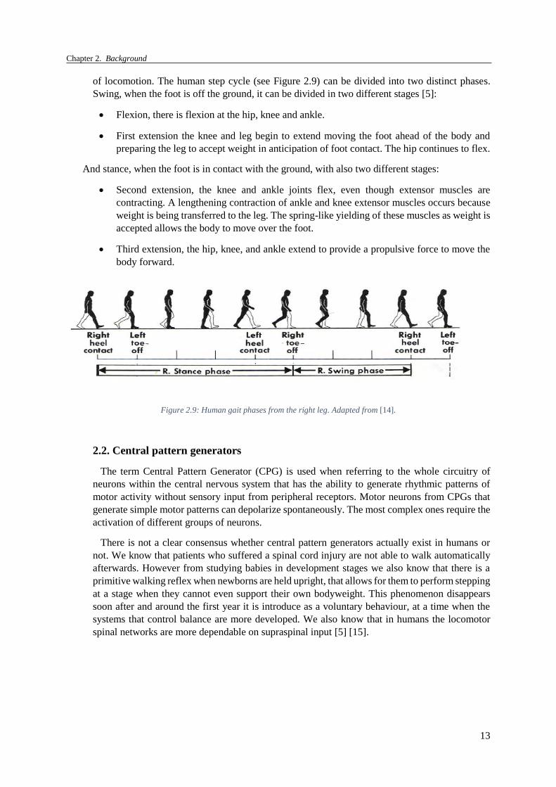
of locomotion. The human step cycle (see Figure 2.9) can be divided into two distinct phases.

Swing, when the foot is off the ground, it can be divided in two different stages [5]:

Flexion, there is flexion at the hip, knee and ankle.

First extension the knee and leg begin to extend moving the foot ahead of the body and

preparing the leg to accept weight in anticipation of foot contact. The hip continues to flex.

And stance, when the foot is in contact with the ground, with also two different stages:

Second extension, the knee and ankle joints flex, even though extensor muscles are

contracting. A lengthening contraction of ankle and knee extensor muscles occurs because

weight is being transferred to the leg. The spring-like yielding of these muscles as weight is

accepted allows the body to move over the foot.

Third extension, the hip, knee, and ankle extend to provide a propulsive force to move the

body forward.

Figure 2.9: Human gait phases from the right leg. Adapted from [14].

2.2. Central pattern generators

The term Central Pattern Generator (CPG) is used when referring to the whole circuitry of

neurons within the central nervous system that has the ability to generate rhythmic patterns of

motor activity without sensory input from peripheral receptors. Motor neurons from CPGs that

generate simple motor patterns can depolarize spontaneously. The most complex ones require the

activation of different groups of neurons.

There is not a clear consensus whether central pattern generators actually exist in humans or

not. We know that patients who suffered a spinal cord injury are not able to walk automatically

afterwards. However from studying babies in development stages we also know that there is a

primitive walking reflex when newborns are held upright, that allows for them to perform stepping

at a stage when they cannot even support their own bodyweight. This phenomenon disappears

soon after and around the first year it is introduce as a voluntary behaviour, at a time when the

systems that control balance are more developed. We also know that in humans the locomotor

spinal networks are more dependable on supraspinal input [5] [15].


14

2.2.1. Fine control of locomotor patterns

The visual, vestibular and somatosensory systems provide input that is used to regulate

stepping patterns. Proprioceptors in joints and muscles automatically regulate stepping.

Cutaneous receptors in the skin give feedback and adjust the stepping patterns to the environment.

Studies with decerebrated cats show that electrical stimulation of the Mesencephalic

locomotor region (MLR) initiates stepping. The intensity of this stimulation does not modify the

pattern, but the speed of the walk. The mesencephalic motor neurons connect with neurons in the

medullary reticular formation whose axons descend in the ventrolateral region of the spinal cord.

Adrenergic drugs can initiate stepping patterns, but it is not what triggers it in nature.

Administration of glutamate receptor agonists initiate locomotor activity similarly to when the

MLR is stimulated. It is concluded that regarding the descending systems that initiate movement,

glutamatergic pathways are involved.

The cerebellum fine tunes locomotor patterns by regulating the timing and intensity of

descending signals. Neurons in the dorsal tract are strongly activated by numerous leg

proprioceptors and therefore provide the cerebellum with detailed information about the

mechanical state of the hind legs. In contrast, neurons in the ventral tract are activated primarily

by interneurons in the CPG, thus providing the cerebellum with information about the state of the

spinal locomotor network. The cerebellum also receives input from the motor cortex and other

forebrain regions related to locomotor function.

The motor cortex uses visual information in complex stepping patterns (walking in

irregular terrain, stepping over obstacles). A considerable amount of neurons is activated in the

motor cortex, which project to the spinal cord, and may regulate interneurons in the CPG for

locomotion and adjust timing and magnitude of a specific locomotor task.

Planning and coordination of visually guided movements involves the posterior parietal

cortex. Neurons from this structure seem to increase their activity when an animal approaches an

obstacle in their path. For quadrupeds, the posterior parietal cortex stores information in the visual

working memory, in order to regulate hind limb movements since they usually are not in the

animal’s vision field.

Figure 2.10: Functional organization of supraspinal structures in locomotion. Adapted from [5].


15

We can divide supraspinal systems into three different functional areas: one activates the

spinal locomotor system, initiates walking, and controls the overall speed of locomotion; another

one refines the motor pattern in response to feedback from the limbs; and a third one that visually

guides limb movement (see Figure 2.10). Descending pathways are necessary for initiation and

adaptive control of stepping and fine control of stepping movements involves the motor cortex,

cerebellum and various sites in the brain stem.

2.3.Encoding of movement by the motor and premotor cortex

The motor cortex role in the underlying processes of movement is one of supervision, and it is the

highest hierarchical structure of motor related neuronal activity. The firing rates of neurons is well

observed in the motor cortex, especially when multiple muscle groups are required to perform a certain

movement. However, the level of abstraction that we get from looking at this activity is higher in the

motor cortex than it is in other lower levels as the spinal cord.

The firing rates of the three different areas of the motor cortex are associated with specific events.

The neurons from the primary motor cortex fire 5-100 ms before the movement itself and these action

potentials encoded the force, direction, extent and speed of the movement.

The premotor cortex is associated with more complex movements and postures. This area signals

the preparation of movement, various sensory aspects associated with particular motor acts and the

association of contextual external information with specific movements. The supplementary motor area

seems to be connected to the choice of movements based on previously obtained information of

movement sequences. It is involved in the transformation of kinematic information into dynamic

information and in the mental rehearsal of sequences of movements.

3. Spinal cord injury and Neurorehabilitation

Spinal cord injuries are usually the result of trauma or diseases such as polio and spina bifida and

have serious implications on the individual lifestyle and quality-of-life. The type of injury is

denominated by the lowest level of the spinal cord that still has normal function. For example a C4

injury means that above that cervical nerve, all spinal cord nerves are still completely functional and the

referred one included. Figure 2.11 illustrates different sites of injuries and the corresponding degree of

paralysis.


16

Figure 2.11: Diagram of different paralysis types as a result of a SCI. Adapted from [16].

The injury can also be classified as complete or incomplete depending on the degree to which the

spinal cord is severed. If there is still a neural bridge after the injury is considered an incomplete lesion

and if there is no nerve connections left it is a complete lesion. Also, when referring to spinal injuries

there is a distinction between lesions that cause sensory loss and motor loss, since the ventral roots might

be damaged but not at the same level as the dorsal ones or vice versa.

3.1. Clinical neurorehabilitation

A SCI triggers changes within the sensorimotor system. The subsequent impairment depends

on both level and completeness of injury. We will focus on the basic and clinical research to re-establish

sensorimotor systems involved in functional movements.

According to the level of severity of the lesion, there are guidelines for patients to undergo

different available treatments. The rehabilitation goals also differ since it is important to be mindful and

have realistic recovery expectations depending on the lesion characteristics. Figure 2.12, synthesizes the

degree of injury (according to the ASIA scale[17]), the treatment approach and the rehabilitation goals.


17

Figure 2.12: (A) Rehabilitation guidelines after a SCI. Adapted from [17]. (B) Classification of spinal cord injury according to the American Spinal Injury Association. Adapted from [18].

In incomplete injuries, neuroplasticity after SCI plays a major role in the rehabilitation of

functional movements. It occurs at several anatomical levels of the CNS, such as the spinal cord, the

brain stem and the cortex. By unloading the body with assistance, neuroplasticity can be facilitated

through the training of movements and by electrical stimulation techniques. However, proprioceptive

input to the spinal cord is essential when triggering a locomotor electromyographic pattern during

training, since the resulting movements need to evoke appropriate afferent input to the spinal cord to

promote neuroplasticity.

Electrical stimulation of the spinal cord was first introduced as a pain relief treatment. Here, an

electrode array is implanted in the epidural space of the spinal cord connected to a wire that connects to

an electrical impulse generator. It reliefs pain by modifying the pain signal before it reaches the brain.

Not all patients experience the benefits of this treatment. Furthermore, research has shown that epidural

electrical stimulation delivered bellow the site of injury can also trigger locomotor patterns, as discussed

previously on this chapter.

Around sixty percent of patients with SCI have complete injuries[18]. Perspectives for regaining

function in this individuals are less and more complex. Nevertheless some preclinical approaches to

restore function are being researched.

(A)

(B)


18

A complete injury deprives spinal neuronal networks of the descending input that is necessary to

trigger their activation. Studies using animal models show that after complete transection of the spinal

cord, this lack of excitatory drive from supraspinal centres can be compensated pharmacologically, by

electrical stimulation, or by natural sensory afferent input. Even though these studies show promising

results, translation to humans have shown less satisfactory results. Still, these techniques show promise

and an answer may lie in combining them with axonal regeneration tactics[18].

Some approaches to induce neural repair in the spinal cord were moderately successful in rodents.

Schwann cells, which are a type of macroglia cells from the peripheral nervous system, have

demonstrated the ability to form tissue bridges after complete lesions. There have been studies that

reported regeneration of a few millimetres in axons in rodents, which is still a long way from what a

human injured spinal cord needs[18]. In addition, the risk of tumour formation cannot be ignored and

axons need to guaranteedly, form the correct connections.

Although this is a growing field of research, there are many other major challenges surrounding

clinical translation. Most studies in animal models rely on techniques that need incomplete lesions where

there is residual tissue bridges. Also, when it comes to animal models, we see that different species have

different possible degrees of recovery. We know that primates have a higher degree of recovery when

compared to rodents, since their corticospinal tract has a higher degree of midline crossing collaterals

resembling humans better[18]. Finally, quadrupedal locomotion allows for more post-lesion training

activities when compared to human bipedal walking.

3.2.Training, pharmacological treatments and epidural electrical stimulation

Rats with paralyzing lesions showed the ability to exert supraspinally controlled hindlimb

movement after several weeks of training with an electrochemical neural prostheses that encouraged

reorganization of the neural circuitry [3]. In addition, Harkema et al. proved in 2011 that epidural

electrical spinal cord stimulation in human patients with complete spinal cord injuries can provide a

certain degree of supraspinal control of the legs. At the end of the trials individuals were able to

voluntary execute toe extension, ankle dorsi-flexion and leg flexion with help of epidural electrical

stimulation[2].

The recruitment of neural pathways is possible with imposed electrical stimulation of the spinal

cord. One of the possible explanations for this is that a combination of chemical drugs and electrical

epidural stimulation of the lumbosacral spinal cord can force the activation of pathways that trigger CPG

networks modulated by sensory information obtained from afferent connections.


19

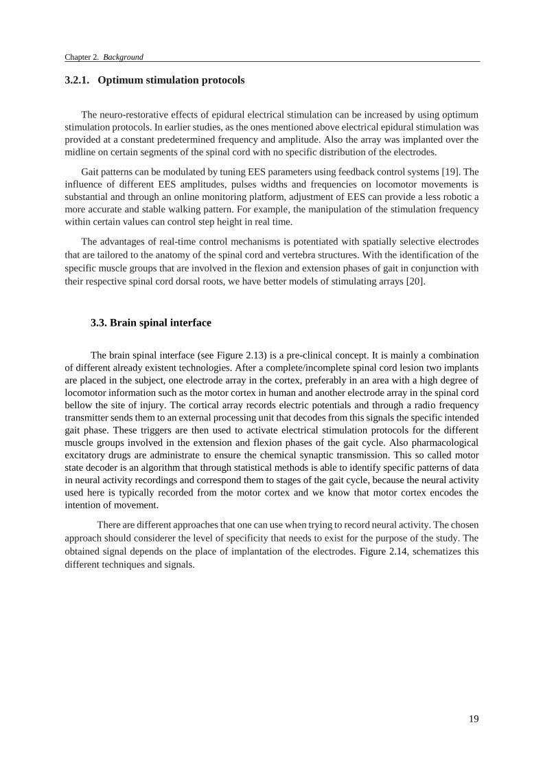
3.2.1. Optimum stimulation protocols

The neuro-restorative effects of epidural electrical stimulation can be increased by using optimum

stimulation protocols. In earlier studies, as the ones mentioned above electrical epidural stimulation was

provided at a constant predetermined frequency and amplitude. Also the array was implanted over the

midline on certain segments of the spinal cord with no specific distribution of the electrodes.

Gait patterns can be modulated by tuning EES parameters using feedback control systems [19]. The

influence of different EES amplitudes, pulses widths and frequencies on locomotor movements is

substantial and through an online monitoring platform, adjustment of EES can provide a less robotic a

more accurate and stable walking pattern. For example, the manipulation of the stimulation frequency

within certain values can control step height in real time.

The advantages of real-time control mechanisms is potentiated with spatially selective electrodes

that are tailored to the anatomy of the spinal cord and vertebra structures. With the identification of the

specific muscle groups that are involved in the flexion and extension phases of gait in conjunction with

their respective spinal cord dorsal roots, we have better models of stimulating arrays [20].

3.3. Brain spinal interface

The brain spinal interface (see Figure 2.13) is a pre-clinical concept. It is mainly a combination

of different already existent technologies. After a complete/incomplete spinal cord lesion two implants

are placed in the subject, one electrode array in the cortex, preferably in an area with a high degree of

locomotor information such as the motor cortex in human and another electrode array in the spinal cord

bellow the site of injury. The cortical array records electric potentials and through a radio frequency

transmitter sends them to an external processing unit that decodes from this signals the specific intended

gait phase. These triggers are then used to activate electrical stimulation protocols for the different

muscle groups involved in the extension and flexion phases of the gait cycle. Also pharmacological

excitatory drugs are administrate to ensure the chemical synaptic transmission. This so called motor

state decoder is an algorithm that through statistical methods is able to identify specific patterns of data

in neural activity recordings and correspond them to stages of the gait cycle, because the neural activity

used here is typically recorded from the motor cortex and we know that motor cortex encodes the

intention of movement.

There are different approaches that one can use when trying to record neural activity. The chosen

approach should considerer the level of specificity that needs to exist for the purpose of the study. The

obtained signal depends on the place of implantation of the electrodes. Figure 2.14, schematizes this

different techniques and signals.


20

In a macroscopic scale, electrodes are placed on top of the skin non-invasively and the

techniques are called electroencephalography and magnetoencephalography which record the signals

through the meninges, skull and skin and therefore implies a high degree of noise and poor resolution,

comparatively. In electroencephalography we have the summed electrical currents associated with the

firing of neurons and in magnetoencephalography the magnetic fields produced by these electrical

currents. In one degree deeper we have electrocorticography where the electrodes are implanted on top

of the meninges that envelope the brain. Another technique is Local Field Potentials where the electrodes

are implanted right on the cortex piercing the nerve cells. The level of resolution is high and the signal

corresponds to the sum of the electrical currents from nearby neurons within a spatial reach of a few

hundred. The frequency range goes from 0.5 Hz to 300 Hz. This signal, as it provides information from

a collective number of neurons, gives us a good understanding of more complex processes and cognitive

functions.

Figure 2.13: Brain spinal interface concept using the rodent model


21

Figure 2.14: Schematics of different neural activity recording techniques. The scale of the recorded neurons increase from left to right. Adapted from [21].

Spikes or action potentials, can also be recorded using microelectrodes. We can refer to them as

single unit when it corresponds to activity from one individual neuron recorded using microelectrodes

or multi-unit when they were recorded using an array of microelectrodes that record from different

neurons. Different techniques are known for the extraction of single unit spikes.

4. Detection algorithms

The motor state decoder is essentially, a predictive algorithm. We can construct a model that has the

ability to make predictions on data using computational statistics. Several science fields specialize in

building and optimizing of these models/algorithms and its applications are numerous. There are mainly

two different types of learning methods that we will consider: supervised learning and unsupervised

learning.

Depending on the type of problem and data, some approaches are more adequate than others, see

Figure 2.15. Supervised learning implies that there is input and output data apriori that will be used to

build the algorithm, and thus will be able to predict new results from unseen new input data. Then

considering whether the desirable output we want to predict is continuous or categorical variables we

have regression or classification methods, respectively. The second type of learning method is

unsupervised learning that does not have the output data as its teacher. This works by clustering the data

[22].

These two types are not completely separate from each other, for example, unsupervised

learning can be used followed by supervised learning [22].


22

Figure 2.15: Schematics showing different types and categories of learning algorithms. Adapted from [23].

23

Chapter 3 : State-of-the-art

State-of-the-art

1. Brain machine interfaces in healthcare

There has been a lot of recent developments in research regarding the control of external devices

using one’s own brain. The applications for these type of devices are extensive and provide a very

important step in medical devices. However the demand and the consequent fast pace of new equipments

and techniques available is not only due to medical purposes but also due to their vast application in

other areas, from gaming devices to security and marketing[24]. Brain computer interfaces (BCIs) for

medical purposes can also be used, as a mean of communication for patients with speech impairments,

or for movement rehabilitation and assistance in patients with movement disabilities. Different types of

invasive and non-invasive neural activity recording techniques can provide us with different types of

signals that contain useful information on neural states. The five types of signals that one can get from

invasive techniques are: Local Field Potentials (LFPs), Single Unit Activity (SUA), Multi-Unit Activity

(MUA), electrocorticographic oscillations (from electrodes on the cortical surface) and calcium channel

permeability[25]. From non-invasive techniques we have seven types of brain signals: slow cortical

potentials, sensorimotor rhythms, P300 event related potential, steady-state visual evoked potentials,

error-related negative evoked potentials, blood oxygenation levels and cerebral oxygenation changes

[26]. These different signals have been widely used and have already reported levels of accuracy and

robustness.

For assistance purposes, most existent studies show the ability of a person or monkey to control or

manipulate a robotic upper limb with previous training sessions where the subject imagines the

movement by looking at a screen demonstration or by observing the robotic component perform it. Brain

computer interfaces can also have an important role in neurorehabilitation when combined with

functional electrical stimulation, since they can therefore provide a bridge between existent supraspinal

commands and efferent nerve fibers.

In 2008, Miller et al showed in monkeys with temporarily paralysed forearm muscles that it was

possible to use recordings from their motor cortex to provide control protocols over functional electrical

stimulation to forearm muscles. A Wiener cascade decoder used approximately 100 neural signals to

predict kinetic forces. A multi-electrode array was implanted in the area that encoded hand movements

information on the primary motor cortex and spike sorting was performed based on the shapes of the

waveforms and inter-spike intervals.

Chapter 3. State of the art

24

In 2016, Bouton et al showed that it was possible, through learning algorithms, to record MUA from

the motor cortex and control forearm muscles using a custom-built neuromuscular electrical stimulation

system (NMES) in a quadriplegic patient[27]. The NMES was an array of 130 electrodes embedded into

a flexible sleeve that was wrapped around the arm (see Figure 3.1). The patient had to do six selected

movements indicated by a computer screen, intercalated with rest periods. One decoder was trained for

each individual task using a support vector machine algorithm.

Figure 3.1: (A) Neuromuscular electrical stimulation system (NMES). Adapted from [27]. (B) Patient with NMES, implanted cortex array and computer monitor giving instructions Adapted from [27].

1.1. Brain spinal interfaces for neurorehabilitation

Very few studies have actually been done, combining brain machine interfaces with functional

electrical stimulation designed for locomotion restoration. In 2014 [28], a brain-machine-muscle neuro-

prosthetic device was attempted and its feasibility tested in six rats. A micro-wire array consisting of

one stimulation array, seven neural recording electrodes, one reference electrode and one common

terminal electrode was implanted. Neural recordings were mainly obtained from layers V/VI of the

motor cortex. Ten to twenty walking sessions with a one minute duration of neural activity were

recorded after the implantation surgery. The rats underwent a second surgery for a spinal cord

transection and after three to four days of recovery they were attached to a body weight support system

which allowed only forelimb walking.

Here a neural signal processing system was built to decode the locomotor primitives form the neural

activity. The system had an online spike detection circuit and a signal processing unit. Various spike

detection methods were implemented, but lastly the one that showed better performance was the median

value spike threshold method. The neuroprocessor run baseline firing rate calculations of the given

signal to obtain the threshold value and when the smoothed average spike count was higher than the pre-

stored threshold count, the system would prompt stimulation procedures, as shown in Figure 3.2. The

electrical stimulation circuit provided biphasic pulses. Different stimulation parameters were tested in

order to find the best ones, which proved to be 3 pulses with frequency of 100Hz, for 0.5 ms time each.

This allowed rhythmic bilateral hind leg movements.

(A) (B)


25

To test this concept, firstly the procedure was done in an offline mode, without using any

stimulation, and the predicted steps were compared to the actual observed steps. Eleven out of fourteen

steps were correctly identified (79% accuracy) with a mean time delay of 113.41 ms. Then in real time

functioning, the decoder could predict and properly stimulate and trigger locomotion. However after the

complete spinal cord transection, accurate locomotor information could no longer be predicted from

neural activity obtained from the primary sensorimotor cortex.

Figure 3.2: (A) Brain-to-muscle interface. Adapted from [28]. (B) A diagram of the program flow chart from brain-to-muscle study. Adapted from [28].

Another brain-spinal interface in monkeys has been successfully developed in the Courtine lab

which translates motor intention from motor cortex signals and triggers electrical spinal cord stimulation

protocols. The concept is described in Figure 3.3, and consists of an e-dura array [29] that records neural

signals and transmits it wirelessly to a computer, that decoded locomotor states and triggers spatially

selective electric current pulses executed by the implanted spinal cord stimulation array in a close loop

system that monitors the subsequent movements and the electromyography signals.

(A)

(B)


26

Figure 3.3: Brain spinal interface developed by the Courtine lab in monkeys.

2. State of the art of motor states detection algorithms

2.1. Extracting neural information on locomotion from cortical recordings in rats

Motor cortical neurons encode different variables that can be used for epidural electrical stimulation

in rodent models. Although Brain-Machine-Interfce(BMI) research has been largely neglected in this

field, some efforts have been made.

In 2009 [30], multiple movement related variables such as robot attachment point position, velocity,

and hind limb state were predicted in rats using regression algorithms. Here, it was found that proximal

variables were better decoded than distal ones, from the motor sensorimotor cortex, having better

kinematics reconstruction at the pelvis level. The study used neural firing patterns has its input

information and experiments were made using four rats walking with a robot attached to their pelvis.

Also the performance of decoding was compared with reported decoding performance from the DRG

neurons and it showed that decoding from the DRG had increased performance, demonstrating that the

activity form cortical neurons is more abstract.


27

In 2012 [31], a study using six rats that had to perform a behavioural task which consisted of pressing

a pedal upon hearing an audio cue, used single neuron activity to predict three events. This events were

the audio cue, the start of the pressing of the button and the end of pressing the button and peri-event

time histograms were used to predict them by showing neuron firing times in a specific time window

around the event. Principal component analysis was previously performed to the data. In addition, the

kinematics of the trajectory performed by the rat during the behavioural task was decoded using a

Wiener filter weighted on the spiking activity of all the neurons recorded simultaneously from the hind

limb sensory motor cortex. The model was trained using 50 % percent of the data and tested on the

remaining 50% using the cross-validation method.

In 2015 [32], another study performed experiments on six rats trying to decoded several movement

related variables from recorded neural activity. These rats were implanted with a recording array in the

left motor cortex which recorded single and multi-unit activity, and also with ten bipolar electrodes in

the hind limb muscles of the right hind limb to view electromyographic signals. The behavioural tasks

were standing, stepping on a treadmill, walking overground and climbing staircases all with a bipedal

posture backed by a body weight support system. Firing rates of stable neural units were used to build

classifiers of gait phases, stance or swing, or types of tasks, treadmill, runway and staircase using the

support vector machine learning method. Also hind limb kinematics gathered as Cartesian coordinates

where decoded using the same method. The study concluded affirming that brain machine interfaces can

be more accurately built by estimating gait phases instead of continuous variables such as limb or joint

positions since they provide more robust control strategies for stimulation protocols.

2.2. Robustness and long-term performance of the decoder

The long-term performance of a decoder depends on the stability of the neural signals used as input

information. The non-stationarity of neural signals presents itself as a challenge when using techniques as spike

sorting, since the shapes of the waveforms of action potentials change over time due to shifts in membrane

conductance’s during extended burst firing sequences and electrode position changes. This makes the case for

further studying the performance of decoders using LFPs and unsorted spikes when decoding movement

variables.

It is reported that LFPs are significantly more stable than spikes[33] but still less accurate. However,

performance of detection algorithms that use LFPs as input neural information is still significant enough

to ensure precise decoding[34].

For regression type problems, the Kalman filter and its optimized versions have the highest

reported communication rate neural prosthesis to date [35], [36]. In terms of motor states classification

problems, the linear discriminant analysis classifier and the quadratic discriminant analysis classifier

have the most consistent performance overall [22], being consistently ranked among the top three

classifiers for multiclass classification.

28

Chapter 4 : Decoding gait phases from LFPs in rats

Decoding gait phases from local field potentials in

rats

As stated in previous chapters, to prove that the BSI was feasible in the rat model we needed to

first, find out if we could build a motor state decoder that from neural activity could decode specific gait

phases accurately.

The cerebral cortex of the human brain is divided into four lobes each responsible for distinct

functions as described in Chapter 2. The frontal lobe houses the motor cortex, which only controls

movement. The rat’s brain is organized in different functional areas from the human brain, and the area

that is known to encode information about movement is the primary sensorimotor cortex represented in

Figure 4.1 by M1.This functional area is the highest hierarchical structure of both motor and sensory

related neuronal activity. For decoding purposes we needed, at least, of local field potentials, so the

cortical implant should be piercing the nerve cells of sensorimotor cortex. Also, since the electrode was

intended to be implanted in the right cortex (which encodes left side locomotor activity), it made sense

to start with the left hind limb. We chose the hindlimb and not the forelimb since the BSI is to be

primarily developed for locomotion restoration and translation must be kept in mind.

Figure 4.1: Rat’s functional brain cortex areas viewed from vertex. The black circle locates the sensorimotor cortex. Adapted

from[37].

Considering the rat step cycling , we choose two key moments, the beginning of the stance phase

where the foot is in contact with the ground, which we called foot strike, and the beginning of the swing

phase where the foot has just left the ground entirely, which we called foot off. In summary, as an input

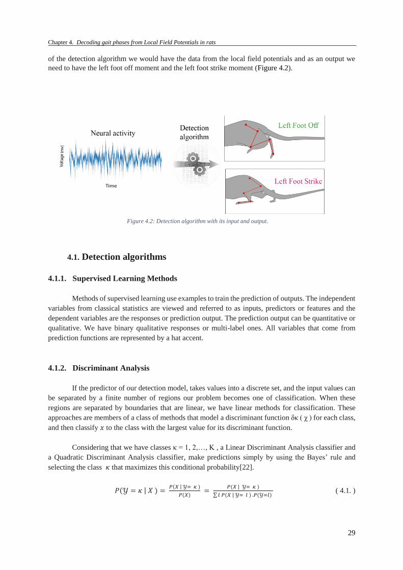
Chapter 4. Decoding gait phases from Local Field Potentials in rats

29

of the detection algorithm we would have the data from the local field potentials and as an output we

need to have the left foot off moment and the left foot strike moment (Figure 4.2).

4.1. Detection algorithms

4.1.1. Supervised Learning Methods

Methods of supervised learning use examples to train the prediction of outputs. The independent

variables from classical statistics are viewed and referred to as inputs, predictors or features and the

dependent variables are the responses or prediction output. The prediction output can be quantitative or

qualitative. We have binary qualitative responses or multi-label ones. All variables that come from

prediction functions are represented by a hat accent.

4.1.2. Discriminant Analysis

If the predictor of our detection model, takes values into a discrete set, and the input values can

be separated by a finite number of regions our problem becomes one of classification. When these

regions are separated by boundaries that are linear, we have linear methods for classification. These

approaches are members of a class of methods that model a discriminant function δκ ( χ ) for each class,

and then classify 𝑥 to the class with the largest value for its discriminant function.

Considering that we have classes κ = 1, 2,…, K , a Linear Discriminant Analysis classifier and

a Quadratic Discriminant Analysis classifier, make predictions simply by using the Bayes’ rule and

selecting the class 𝜅 that maximizes this conditional probability[22].

𝑃(𝒴 = 𝜅 | 𝑋 ) = 𝑃(𝑋 | 𝒴= 𝜅 )

𝑃(𝑋) =

𝑃(𝑋 | 𝒴= 𝜅 )

∑ 𝑙 𝑃(𝑋 | 𝒴= 𝑙 ) .𝑃(𝒴=𝑙) ( 4.1. )

Figure 4.2: Detection algorithm with its input and output.


30

𝑃( 𝑋 | 𝒴 = 𝜅 ) is modelled as an estimated multivariate Gaussian distribution [22]with a

density function of

𝑃( 𝑋 | 𝒴 = 𝜅 ) = 1

(2𝜋)𝑛| ∑ ℎ1/2𝜅 |

exp(−1

2 (𝑋 − 𝜇𝜅)𝑡 ∑ ( 𝑋 − 𝜇𝜅 ) )−1

𝜅 ( 4.2. )

𝜇𝜅 - mean of each class,

∑ 𝑓−1𝜅 - inverse covariance matrix.

The mean of the class distribution is estimated by the class sample mean and the covariance by

the class sample covariance, in the following way[22]

𝜇 ̂ = 1

𝑁∑ 𝑥𝑛𝑁

1 ( 4.3. )

∑ ̂ = 1

𝑁∑ (𝑥𝑛 −𝑁

𝑛−1 𝜇 ̂) (𝑥𝑛 − 𝜇 ̂)𝑇 ( 4.4. )

N – sample size.

For the linear discriminant analysis classifier (LDA) the classes share a covariance matrix which

makes the decision boundary surface linear. The quadratic discriminant analysis (QDA) model assumes

that the classes are conditionally independent since the covariance matrices are diagonal and generates

quadratic boundaries between classes[22]. To classify new data we can apply each of the class Gaussian distributions and calculate the

probability. To determine the correspondent class we either chose the class with the highest probability

or use a threshold value.

4.1.3. Stability and accuracy of LDA and QDA

The LDA and the QDA classifiers have good track records. Both techniques are widely used

and produce stable results. The reasoning for this might be that the data supports better, simple decision

boundaries. This favours these methods that have linear and quadratic boundaries, respectively,

assuming that the Gaussian distribution is stable[22].

4.1.4. Regularized Discriminant Analysis

When our number of features is much higher than our number of samples we have a high

dimensionality problem, which can cause overfitting and high variance problems. To overcome this

issue we can use a linear classifier with quadratic regularization. Because the dimension of the

covariance matrix is 𝑋 𝜌 , where 𝜌 is the feature dimension, in cases where the features’ dimension is

much bigger than the number of samples the covariance matrix becomes singular. To correct this we

use regularization to shrink ∑̂ towards its diagonal.


31

Σ̂(𝛾) = (1 − 𝛾) Σ̂ + 𝛾 𝑑𝑖𝑎𝑔(Σ̂) ( 4.5. )

𝛾𝜖[0,1].– regularization coefficient,

Σ̂ – covariance matrix.

In this technique, the regularization parameter is usually computed using a cross-validation

procedure, which searches the classification accuracy using a finite range of γ values and finds the value

in this range that maximizes it.

4.1.5. Cross-Validation

Cross-validation is the most widely used method for estimating prediction error. Typically estimates

well only the expected prediction error.[22] K-fold cross-validation uses a part of the data to fit the

model and another part to test it, computing the prediction error of the fitted model. The original dataset

is divided into equal k=1,2,..N folds and t folds are used for training the model and the other N-t are

used for validating the model. N is the total number of trials. Every data fold is used for validating the

model through different iterations and at the end the error is estimated conjointly. Figure 4.3 shows an

example of a dataset division where N=4 and k=2.

1 2 3 4

Training set Training set Validation set Validation set

1 2 3 4

Validation set Validation set Training set Training set

Figure 4.3: Example of a dataset division for the purposes of cross-validation.

When choosing the size of the training set, we know that if k=N it is unbiased for the true

prediction error but has high variance and the computational time is high. However, if we considerably

decrease k, we have lower variance but bias is a problem. Figure 4.4 shows in a hypothetical situation

how the choice of k, and subsequently of the training set size, can overestimate the expected error. The

final compromise is taken when considering the goal of the study.


32

Figure 4.4: Learning curve for a classifier with 200 observation. Err is the estimated average error. Adapted from [22].

4.1.6. Mutual information value

Although we can use the conventional prediction error as a value of the accuracy of the model

we can also calculate directly its performance by measuring the mutual information value that compares

the time of real events and the time of detected events from one dataset. The mutual information value

is given by,

𝐼(𝑋, 𝑌) = ∑ ∑ 𝑝(𝑥, 𝑦) log2(𝑝(𝑥,𝑦)

𝑝(𝑥)𝑝(𝑦))𝑌𝑋 ( 4.6. )

X, Y – sets of all possible states of real and detected events

𝑝(𝑥, 𝑦) – joint probability of x and y happening jointly

𝑝(𝑥) and 𝑝(𝑦) – probability of specific event.

It ranges from 0 to 1, and the maximum is achieved when the detected events and real events

perfectly match within a chosen time window.

33

Chapter 5 : Methods

Methods

1. Rat model and surgical procedures

As mentioned before the rat animal model was suitable for this study due to its accessibility to

a range of immunohistochemistry techniques needed to explore the levels of neural restoration. Two

female Lewis rats designated by r263 and r328, were used for the experiments. Under general anesthesia,

a craniotomy was performed over the right sensorimotor cortex. A ZIF-Clip, 32-channel microelectrode

array (Tucker-Davis Technologies (TDT), Alachua, FL, USA) was inserted with the help of a hydraulic

33 microdrive using stereotaxic coordinates and spatio-temporal neuronal characteristics to localize

layer V. The row spacing of the microwire array was 250 μm, while the column spacing was 375 μm.

To ensure fixation to the skull cranial screws and dental cement were placed. The wires were

subsequently covered with dental cement. The array component that connects to the headstage of the

ZIP-Clip was left uncovered and projected upwards. Also bipolar electrodes were implanted into the

hindlimb muscles in order to record electromyography activity.

All procedures were conducted in accordance with Swiss federal legislation and under

guidelines established at EPFL, and approved by local Swiss Veterinary office.

2. Acquisition system

The headstage component was connected to a dedicated neurophysiology RZ5 workstation

(TDT, Alachua, FL, USA). Here the pre-amplifier had a high-pass filter at 3Hz. The signals were

digitized with a 16 bit resolution at approximately 12 kHz and stored not synchronously with other data.

Whole body kinematics was recorded using the high-speed motion capture system Vicon from Vicon

Motion Systems®, which combines 12 infrared cameras (200 Hz). Reflective markers were placed in

both right and left hindlimbs, positioned on the crest, hip, knee, ankle and fifth metatarsal, making a

total of 10 markers. The 3D kinematics reconstruction was done offline with the help of the Vicon Nexus

software. The electromyography signals were amplified and band pass filtered, however for this study

they were not used therefore not analysed.

The staging of this experiment was already a key feature of the laboratory, which combines all

the before mentioned acquisition systems and inter usable task specific modules. In this case only a 1.5

meters length horizontal runway was necessary.

3. Training and overground recordings

Before surgery each rat was handled for one week in order to get accustomed to the laboratory

environment, runway and human interaction. After surgery both rats underwent several sessions of

recordings after some necessary recovery time. One session consisted of a rat performing a full length

runway quadruple walk using motivation from the trainer when needed. The data from each session was

stored for offline use and at this initial stage a low pass 5khz filter was applied before saving, using the

Matlab® software. At the end, the data used for the duration of the study was from the best data set

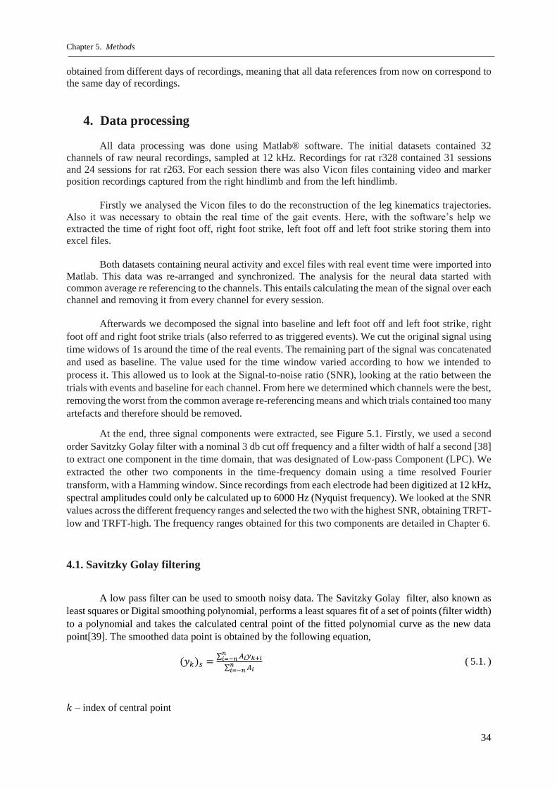
Chapter 5. Methods

34

obtained from different days of recordings, meaning that all data references from now on correspond to

the same day of recordings.

4. Data processing

All data processing was done using Matlab® software. The initial datasets contained 32

channels of raw neural recordings, sampled at 12 kHz. Recordings for rat r328 contained 31 sessions

and 24 sessions for rat r263. For each session there was also Vicon files containing video and marker

position recordings captured from the right hindlimb and from the left hindlimb.

Firstly we analysed the Vicon files to do the reconstruction of the leg kinematics trajectories.

Also it was necessary to obtain the real time of the gait events. Here, with the software’s help we

extracted the time of right foot off, right foot strike, left foot off and left foot strike storing them into

excel files.

Both datasets containing neural activity and excel files with real event time were imported into

Matlab. This data was re-arranged and synchronized. The analysis for the neural data started with

common average re referencing to the channels. This entails calculating the mean of the signal over each

channel and removing it from every channel for every session.

Afterwards we decomposed the signal into baseline and left foot off and left foot strike, right

foot off and right foot strike trials (also referred to as triggered events). We cut the original signal using

time widows of 1s around the time of the real events. The remaining part of the signal was concatenated

and used as baseline. The value used for the time window varied according to how we intended to

process it. This allowed us to look at the Signal-to-noise ratio (SNR), looking at the ratio between the

trials with events and baseline for each channel. From here we determined which channels were the best,

removing the worst from the common average re-referencing means and which trials contained too many

artefacts and therefore should be removed.

At the end, three signal components were extracted, see Figure 5.1. Firstly, we used a second

order Savitzky Golay filter with a nominal 3 db cut off frequency and a filter width of half a second [38]

to extract one component in the time domain, that was designated of Low-pass Component (LPC). We

extracted the other two components in the time-frequency domain using a time resolved Fourier

transform, with a Hamming window. Since recordings from each electrode had been digitized at 12 kHz,

spectral amplitudes could only be calculated up to 6000 Hz (Nyquist frequency). We looked at the SNR

values across the different frequency ranges and selected the two with the highest SNR, obtaining TRFT-

low and TRFT-high. The frequency ranges obtained for this two components are detailed in Chapter 6.

4.1. Savitzky Golay filtering

A low pass filter can be used to smooth noisy data. The Savitzky Golay filter, also known as

least squares or Digital smoothing polynomial, performs a least squares fit of a set of points (filter width)

to a polynomial and takes the calculated central point of the fitted polynomial curve as the new data

point[39]. The smoothed data point is obtained by the following equation,

(𝑦𝑘)𝑠 =∑ 𝐴𝑖𝑦𝑘+𝑖

𝑛𝑖=−𝑛

∑ 𝐴𝑖𝑛𝑖=−𝑛

( 5.1. )

𝑘 – index of central point

Chapter 5. Methods

35

𝑛 – number of points to the left and right of central point

𝐴𝑖 – weighting coefficients of polynomial

(𝑦𝑘)𝑠 - new smoothed data point.

This filter doesn’t have its properties defined in the Fourier domain, and derives directly from a

particular formulation of the data smoothing problem in the time domain. However its smoothing

operation of this filter reduces the high-frequency components of the signals and passes the low-

frequencies with little change. This algorithm is not very aggressive, therefore doesn’t cause a significant

loss of information.

4.2. Time resolved Fourier Transform

The Fourier transform decomposes a signal in time into a function of frequencies, extracting

series of cosines and sines which compose the function. The fast fourier transform (FFT) is a discrete

fourier transform algorithm which reduces the number of computations needed to obtain the frequency

domain representation of the original signal [40].

The signal from each session underwent the fast fourier transform in chunks of 1/6 of a second

with a Hamming window that slid according to a step value that was half the window size for baseline

and for the triggered parts of the signal a step of 1/64 seconds.

A Hamming window is defined by the following equation,

𝑊(𝑛) = 𝛼 − 𝛽 cos (2 𝜋𝑛

𝑁) , 0 ≤ 𝑛 ≤ 𝑁 ( 5.2. )

with α = 0.54 and β = 0.46 and a window length of 𝐿 = 𝑁 + 1, and N the number of samples and 𝑛 the

individual elements[40].

After a time resolved Fourier Transform, the amplitudes of every frequency bin are normalized

by dividing them by the average baseline amplitude of the same frequency bin in the respective

session[41].

5. Signal-to-noise ratio analysis

The metric used to compare each of the four triggered related neuronal activities and the baseline

neuronal activity was the signal-to-noise ratios (SNR). This was calculated in the following way,

𝑆𝑁𝑅 (𝑡, 𝑐ℎ) 𝐸𝑉𝐸𝑁𝑇 𝑉𝑆

𝐵𝐴𝑆𝐸𝐿𝐼𝑁𝐸

=|𝜇𝐸𝑉𝐸𝑁𝑇 (𝑡,𝑐ℎ) −𝜇𝐵𝐴𝑆𝐸𝐿𝐼𝑁𝐸|

𝜎𝐸𝑉𝐸𝑁𝑇(𝑡,𝑐ℎ)+ 𝜎𝐵𝐴𝑆𝐸𝐿𝐼𝑁𝐸 ( 5.3. )

t – Time within the event time window,

𝑐ℎ - channel,

𝜇𝐸𝑉𝐸𝑁𝑇 - mean of respective event neuronal activity,

𝜇𝐵𝐴𝑆𝐸𝐿𝐼𝑁𝐸 – mean of baseline neuronal activity,

Chapter 5. Methods

36

𝜎𝐸𝑉𝐸𝑁𝑇 – standard deviation of respective event neuronal activity,

𝜎𝐵𝐴𝑆𝐸𝐿𝐼𝑁𝐸 – standard deviation of baseline neuronal activity.

Figure 5.1: Schematics of Data Processing methods

Chapter 5. Methods

37

6. Extracted features and classification

The goal was to classify 3 different classes of data, left foot off, left foot strike and baseline. We

had 93 different features from each event, since we extracted 3 different components from the original

signal that was recorded over 32 channels, and one channel was removed in order to ensure linear

independency, leaving 31 channels. We took 15 equidistant time points of the signal starting 250 ms

prior to each event and ending at the time of the event, making 1395 different values for each class, see

Figure 5.2. We calculated each class mean and respective standard deviation and obtained the z-scores,

using the following equation.

𝑍 =𝑋−𝐸(𝑋)

𝜎(𝑋) ( 5.4. )

𝐸(𝑋) – mean of the population

𝜎(𝑋) – standard deviation of the population

As this classifier is built by fitting a multivariate Gaussian distribution to each of the classes,

see equation 4.2., we calculated the estimated mean (equation 4.3.) and covariance matrix (equation

4.4.) that underwent a regularization procedure, see equation 4.5, to improve its accuracy in a new

independent dataset.

We obtain the class probabilities for each event, choosing a threshold value of 0.95 as the

probability which represented the occurrence of the events, also ensuring that a refractory period of 150

ms was respected, so that the detection of events would only be quantified if the same class event hadn’t

been detected within that specified period. Figure 5.2 outlines the classification procedures described.

Chapter 5. Methods

38

Figure 5.2: Classification procedures.

Chapter 5. Methods

39

7. Model selection and Cross-validation

The cross-validation was performed three times. We divided the entire dataset into two, three

and ten equally sized parts, and did the whole procedure for the three different divisions in search for

the best model. For each data division we held out one part for the testing set and used the rest for the

training set, see Figure 5.3, and then we looped trough the parts, to change the part which was used as

the testing set.

To find the best prediction model, we trained classifiers with different combinations of model

parameters, namely: feature length values, ranging from 0 ms to 1000 ms; number of features from each

channel, 1 to 15 points; regularization coefficients, ranging from 0 to 1. Each combination was trained

on the training trials and tested on the testing trials, where the cardinal number for true positives, false

positives, false positives and false negatives was saved. After all the iterations we calculated the

combined mutual information value (see equation 4.6.). The mutual information value infers to the

number of detected events within a specific tolerance window around the time of the real event, which

stretched from 10 to 60 ms.

The best prediction model and set of parameters, was found by finding the highest mutual

information value obtained.

Figure 5.3: Part 1 represents Cross-validation procedures and part 2 the selection of the optimum detection model.

Chapter 5. Methods

40

8. Time correction

After choosing the optimal prediction model, we searched for the difference that still remained

between our decoded events and real events. This difference was calculated as the median of all the

differences of same sequenced events. For both rats there was still a significant difference, smaller than

the 60 ms window however, still significant enough considering that a gait cycle was around 250 ms. In

order to correct this we implemented this time bias into the triggers array that was used to train the

classifier, by incrementing it. Afterwards a new model was formed, which accounted for the default

difference.

41

Chapter 6 : Results

Results

1. Extracted features from recorded neuronal activity

A preliminary overview of the signals across the channels showed that it would be difficult to use

spiking activity as input data into the decoder since it didn’t seem to show any recognisable spiking

activity patterns around the time of each event. Other, non-related-to-gait-activity patterns were clearly

superimposed.

Looking at the spectrograms of the trials, which corresponds to the signal around the time of the event,

per channel, we saw the need to remove some abnormal channels from the common average referencing

procedure. For r263, we removed channel 13 and 30. For r328, channel 32 was removed and also session

2 was removed since it showed too many artefacts, see Appendix A.1.

After extracting the two different components (one through the low pass filter and another from the

TRFT, see Methods), we looked at the SNR values of each component for every channel around the

triggers, in order to determine whether or not both components showed relevant and therefore usable

information for the four events, in the context of our problem. The SNR values of all four events from

the two components, for both rats are in Appendix A.2.1. and in Appendix A.2.2.

From the component that was obtained after performing a time resolved fourier transform to the data,

we extracted other two components, with different frequency ranges, by looking at the SNR averaged

over all channels and conditions across all frequency bands. The maximum values at the lower end of

the spectrum identified the TRFT-low frequency range, and the maximum values at the higher end of

the spectrum identified the TRFT-high frequency range. Below, in Figure 6.1 and Figure 6.2 is plotted

the SNR averaged over all channels and conditions of a specific bottom and top frequency. In Table 6.1,

the frequency ranges for TRFT-low and TRFT-high for both rats are listed. For r263 the SNR maximum

was between 3 and 15 Hz for the TRFT-low, and for the TRFT-high it was between 39 and 747 Hz. The

SNR maximum for r328 was 3 to 21 Hz for the TRFT-low and 105 to 693 Hz for the TRFT-high.

Table 6.1 : Frequency ranges for the TRFT-low and TRFT-high, for r263 and r328

TRFT-low TRFT-high

r263 3 - 15 Hz 39 -747 Hz

r328 3 - 21 Hz 105 - 693 Hz

Chapter 6. Results

42

Figure 6.1: Frequency band SNR averaged over all channels and conditions of r263

Figure 6.2: Frequency band SNR averaged over all channels and conditions of r328

Chapter 6. Results

43

2. Decoding left side events

2.1. Model selection and cross-validation

The iterations to determine which model gave a higher mutual information value were performed

by the methods described above. The various values of mutual information and their various

corresponded combinations for rat 328 and 263 left side events decoding, are shown in Appendix B.1. .

From the parameters tested we inferred which combination or combinations corresponded to the

model that allowed the highest mutual information value. For the left side events of rat 263, Table 6.2

shows the parameters values and its mutual information value, which corresponded to the maximum

mutual information value found.

Table 6.2: Optimum combination of parameters for decoding model, of rat 263 left side events, and its mutual information

value.

Division of data in 3 parts

r263

Feature Length (ms) 250

Number of features from

each channel

15

Regularization coefficient 0

Mutual Information Value

using a 60 ms tolerance

window

0.3966

As for the left side events of rat 328 there was more than one combination (see Table 6.3) for the

maximum value therefore the choice fell upon the one that required a lower computational time, since

the division in 10 parts required more than triple the time than the one using thirds of the data, during

cross-validation procedures.

Table 6.3: Optimum combination of parameters for decoding model, of rat 328 left side events, and its mutual information

value and computation time.

Division of data in 3 parts Division of data in 10 parts

r328

Feature Length (ms) 250 250


each channel

15 15

Regularization coefficient 0 0



window

0.6017 0.6017

Computational Time medium high

Chapter 6. Results

44

2.2. Time correction

Lastly, after the appropriate model was built we determined if there still was a difference between the

real events time and the time of the detected events. Both rats still exhibit a significant difference, as it

is described in Table 6.4, calculated as described in the above Methods correspondent section.

Table 6.4: List of time values that correspond to the difference between the time of the real events and the detected events

time, for left foot off and left foot strike.

Left foot off Left foot strike

r263 25 ms 30 ms

r328 25 ms 25 ms

This time values were implemented as a time bias correction variable and the new classification

model was tested again for the time bias between the real and detected triggers.

Table 6.5: List of time values after first time correction that correspond to the difference between the time of the real events

and the detected events time, for left foot off and left foot strike.

Left foot off Left foot strike

r263 0 ms 0 ms

r328 0 ms 0 ms

2.3. Decoding left foot off and left foot strike

After building the decoding model and optimizing it, it is time to put it to action. By showing the

class probabilities correspondent to the left foot off and left foot strike as an independent variable

dependent on time and the chosen threshold of 0.95 we obtained the decoded events (explained in the

Methods section above). In order to have a visual guide of how well the decoded events match the real

events and to look for error anomalies we overlapped the decoded events with the correspondent real

events. In Figure 6.3 and Figure 6.4 we can see four sessions that exemplify the output of the decoder

from rat 263 and 328.

Chapter 6. Results

45

Figure 6.3: Class Probabilities of left side events from rat 263

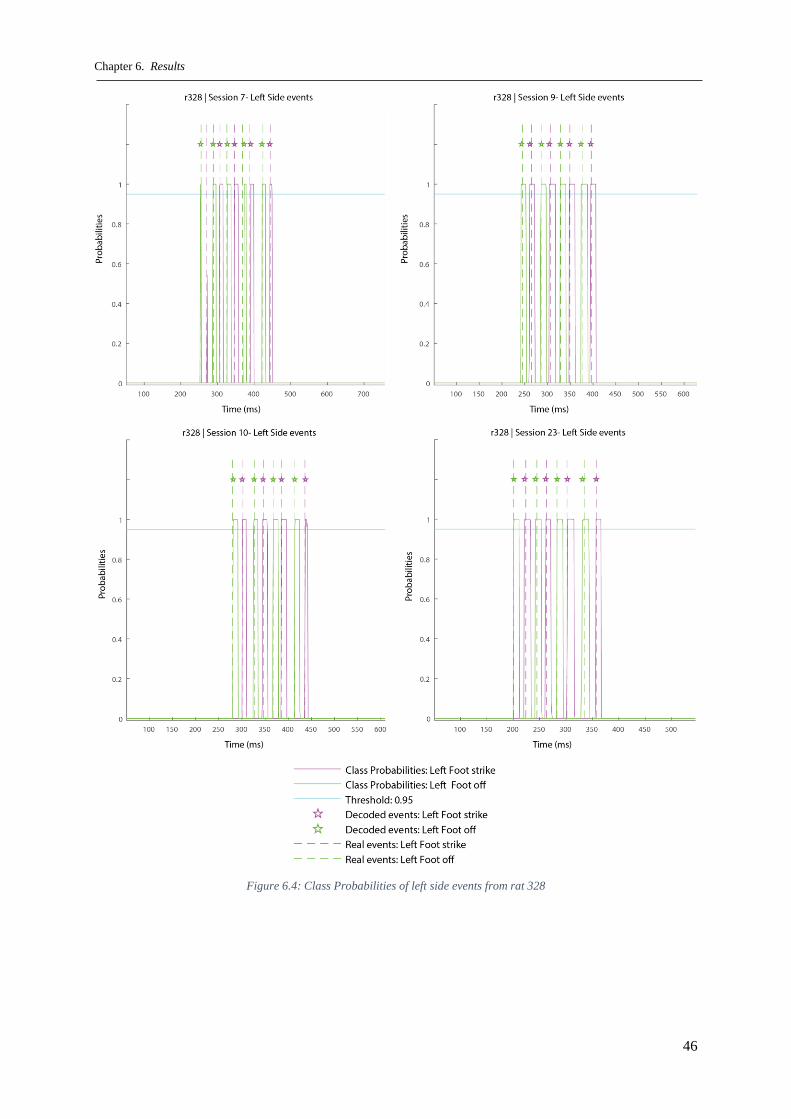
Chapter 6. Results

46

Figure 6.4: Class Probabilities of left side events from rat 328

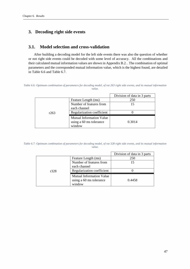
Chapter 6. Results

47

3. Decoding right side events

3.1. Model selection and cross-validation

After building a decoding model for the left side events there was also the question of whether

or not right side events could be decoded with some level of accuracy. All the combinations and

their calculated mutual information values are shown in Appendix B.2. . The combination of optimal

parameters and the corresponded mutual information value, which is the highest found, are detailed

in Table 6.6 and Table 6.7.

Table 6.6: Optimum combination of parameters for decoding model, of rat 263 right side events, and its mutual information

value.


r263



each channel

15




window

0.3014

Table 6.7: Optimum combination of parameters for decoding model, of rat 328 right side events, and its mutual information

value.


r328



each channel

15




window

0.4458

Chapter 6. Results

48

3.2. Time correction

The time correction made concerning the right side events calculated as describe in the Methods

section of the detected events is specified in Table 6.8.

Table 6.8: List of time values that correspond to the difference between the time of the real events and the detected events

time, for right foot off and right foot strike.

Right foot off Right foot strike

r263 40 ms 20 ms

r328 25 ms 30 ms

Identically to the left side events the time differences were tested a second time and the values

obtained are in Table 6.9.

Table 6.9: List of time values after first time correction that correspond to the difference between the time of the real events

and the detected events time, for right foot off and right foot strike.

Right foot off Right foot strike

r263 -5 ms 5 ms

r328 0 ms 0 ms

3.3. Decoding right foot off and right foot strike

The class probabilities of the right side events across time are in Figure 6.5 and Figure 6.6. There

we can see the class probabilities, the decoded events and the real events. Out of the 4 sessions shown,

there is one error from each rat. Both errors occur in the beginning of session 4 (see Figure 6.5) and

session 13 (see Figure 6.6).

Chapter 6. Results

49

Figure 6.5: Class Probabilities of right side events from rat 263. The grey arrow points to a classification mistake.

Chapter 6. Results

50

Figure 6.6: Class Probabilities of right side events from rat 328. The grey arrow points to a classification mistake.

51

Chapter 7 : Discussion and Conclusion

Discussion and Conclusion

State of the art neuro rehabilitation techniques have major potential in surpassing the own body’s

ability to recover from motor impairment due to nerve damage. One technique that has showed clinical

efficacy in humans is epidural electrical stimulation with aid of pharmacology which works by

promoting nerve’s plasticity and therefore creating new nerve circuitries. In this thesis we explore the

feasibility of a system that delivers time and space specific epidural electrical stimulation, focusing on

obtaining proof of concept that we can obtain reliable locomotor primitives from neural activity that can

be used to trigger this stimulation in rats. For this we recorded local field potentials from rats during gait

and used it to train a predictive algorithm offline.

1. Extracted features from recorded neuronal activity

An initial overview of the raw LFPs that were recorded showed a very irregular signal with multiple

artefacts that needed pre-processing. Considering that this signal was recorded from the sensorimotor

cortex, an area that comprises both sensory and motor information this was somewhat to be expected.

Data that corresponded to a time of an event would inescapably not only encode gait primitives but all

sorts of concurrent sensory stimulus. However, since the algorithm is built on existing patterns, this does

not by itself determine the usefulness of the data.

Firstly the signal was divided into two different components (see Methods) and we compared all the

trials correspondent to each of the four events (LFO, LFS, RFO and RFS) to each other and baseline

(Appendix A). It was possible to see a pattern in the neural activity values around the time of the event,

although not always so evident. Also looking at the SNR we can identify the channels that give us the

most information, by looking at the channels that had the highest SNR values, meaning that they had a

higher difference from the baseline values. For r263 these were channels 15, 21, 29 and 31 and for r328,

channels 17, 18, 28 and 30. Figure 7.1 shows the electrode sitemap and the location for these channels.

Considering the small scale of the device and the animal model brain it is not possible to determine

where these electrode locations refer to, in the sensorimotor cortex, without a posterior cortex dissection.

Furthermore we see that RFO and LFS and that LFO and RFS overlap which makes sense considering

the gait cycles phases.

Chapter 7. Discussion and Conclusion

52

Figure 7.1: (A) Site map for electrodes of cortical microarray implanted in r263.The red circles show the channels with the

highest SNR values. (B) Site map for electrodes of cortical microarray implanted in r328.The red circles show the channels

with the highest SNR values. Adapted from [42]

Finally, we extracted two different signal components from the TRFT data, by searching which

frequencies ranges showed the highest SNR. These frequencies are described in Table 6.1. Looking at

the frequency values we see that the TRFT-low range (3~21Hz) covers two known motor-related brain

wave oscillations in rats, beta (12 – 40 Hz)[43] and theta (4 – 8 Hz)[44]. On the other hand the TRFT-

high range (39 ~700 Hz) matches the gamma wave band (30 Hz - 100 Hz)[45]. This neural wave has

also been associated with various cognitive and motor functions.

When comparing the LPC, TRFT-low and TRFT-high spectrograms we see that TRFT-low seems

to show more information around the time of the event, then the TRFT-high and finally the LPC, see

Figure 7.2. Although this is an exception to the rule since the highest frequency component usually can

give us the most information.

(A) (B)


53

Figure 7.2: All trials from LFO and LFS after extracting the three signals (the LPC, the TRFT-low and the TRFT-high) from

the raw neural activity of r328, channel 18.

2. Decoding performance

Four different decoding algorithms were built, one for each rat left/right side events. At end when

searching for the optimum parameters that gave us a higher value of mutual information, see Appendix

B, we realise that they are essentially the same parameters, independent of the subject and side. However

this is a particularity of the data that we had, so we cannot make a generalisation.

The mutual information values regarding the decoding from left and right side, of both rats (see

Table 6.2, Table 6.3, Table 6.6 and Table 6.7) tell us that the decoding algorithm is more accurate for

the left side events than for the right side events. The implanted array that recorded the neural signals

was placed in the right motor cortex in both rats, which therefore implies that there is more information

in the signal regarding activity from the left motor system due to the pyramidal decussation which

changes the side of the encoding pathways from the sensorimotor cortex.

Additionally there is also a significant difference between the mutual information values from r263

and r328, see Table 7.1. The reason for this can be extrapolated from watching the recording videos

provided by the Vicon system, where we can clearly see that r263 had a more lethargic and irregular

gait pattern than r328. The video frames show a much more steady and strong gait from r328.

An analysis to some of the most common misclassification errors shows that they occur at the

beginning or very end of the session or in between extremely close succession of detections. These type

of errors that usually happen at the beginning or end of every session relate to times when the rat would

move his hindlimb legs to accommodate his posture and without necessarily performing a complete step

cycle with a swing and stance stage. As for the second case, when events happened too close to each

other there was a higher risk of misclassification happening, denoting that some event related

information was being masked and maybe a setup of 32 electrodes was not enough.

As for the time bias that the decoder showed (see Table 6.4 and Table 6.8) where the detected events

appeared between 25 ms to 30 ms before the actual events on average, can be intuitively justified by the

fact that the neural activity encoded the intention of movement and not the physical execution of it.


54

Table 7.1: Comparison between mutual information values

Relative difference between

mutual information value from

left and right side events of

r263



left and right side events of

r328

24% 25 %



r263 and r328, left side events



r263 and r328, right side events

34% 32%

3. Future developments

It is possible to accurately decode the two stages of gait from the neural activity of an intact rat,

however the algorithm has still its weaknesses. The overall highest value of mutual information obtained

was 0.6017, which means that around forty percent of the events are still not being accurately detected.

This can be improved by working on a better detection model and by using more data to train and test

it, preferably from multiple days of recording.

Future work on the rat BSI, moving from just proof-of-concept would imply building a decoder on

healthy rats, then performing a lesion and finally providing epidural stimulation controlled by

stimulation protocols triggered by the decoded locomotor primitives. Also the possibility of building a

decoder which could detect the four events should be tested. This was tested in the development of this

project however this work was not carried out because the primary goal was to focus on each individual

side, although it showed promise.

The idea of a brain-machine interface for restoration of hindlimbs or forelimbs has been widely

researched in this past years though not all research focuses on restoration by promoting new circuitry

using existing undamaged neurons. We are confident on the pursuit of this path since it has already

proven efficacy. Nevertheless it is important to better understand how all systems integrate to guarantee

motor functions in a healthy state in order to deal with neuropathologies that compromise them. So,

further and more extensive studies on animal subjects need to happen, such as rats and mice, since they

are more cost and time effective and provide more access to a wider range of immunohistochemistry

techniques. Still, translation has to be kept in mind and additional studies need to be implemented in

human subjects with different degrees of incomplete and complete lesions to answer the question if

space and time-specific stimulation, with aid of pharmacology, provide a more efficient and effective

epidural electrical stimulation with clinical significance than other neuron regenerative techniques.

55

References

[1] P. T. Trent Stephens Rod Seeley, Essentials of Anatomy and Physiology. McGraw-Hill

Science/Engineering/Math; 6 edition, 2006.

[2] S. Harkema, Y. Gerasimenko, J. Hodes, J. Burdick, C. Angeli, Y. Chen, C. Ferreira, A. Willhite,

E. Rejc, R. G. Grossman, and others, “Effect of epidural stimulation of the lumbosacral spinal

cord on voluntary movement, standing, and assisted stepping after motor complete paraplegia: a

case study,” The Lancet, vol. 377, no. 9781, pp. 1938–1947, 2011.

[3] R. Van Den Brand, J. Heutschi, Q. Barraud, J. Digiovanna, K. Bartholdi, M. Huerlimann, L.

Friedli, I. Vollenweider, E. M. Moraud, S. Duis, N. Dominici, S. Micera, P. Musienko, and G.

Courtine, “Restoring Voluntary Control of Locomotion after Paralyzing Spinal Cord Injury,”

Science, vol. 336, no. 6085, pp. 1182–1185, 2012.

[4] M. Capogrosso, T. Milekovic, D. Borton, F. Wagner, E. M. Moraud, J.-B. Mignardot, N. Buse,

J. Gandar, Q. Barraud, D. Xing, and others, “A Brain–Spinal Interface Alleviating Gait Deficits

after Spinal Cord Injury in Primates,” Nature, vol. 539, no. 7628, p. 284, 2016.

[5] E. R. Kandel, J. H. Schwartz, T. M. Jessell, S. A. Siegelbaum, and A. J. Hudspeth, Principles of

neural science, vol. 4. McGraw-hill New York, 2000.

[6] “Everything You Need to Know About the Parts of the Brain,” Johns Hopkins Medicine Health

Library. [Online]. Available:

http://www.hopkinsmedicine.org/healthlibrary/conditions/nervous_system_disorders/anatomy_o

f_the_brain_85,P00773/. [Accessed: 11- May- 2017].

[7] “Upper motor neuron,” Wikipedia. Wikimedia Foundation [Online]. Available:

https://en.wikipedia.org/wiki/Upper_motor_neuron. [Accessed: 12- May- 2017].

[8] “Issues | Brain | Oxford Academic,” Oxford University Press. Oxford University Press [Online].

Available: https://academic.oup.com/brain/issue. [Accessed: 10- May- 2017].

[9] “Spinal Cord Vertebrae Anatomy,” Human Anatomy Diagram. 2016 [Online]. Available:

http://human-anatomy101.com/spinal-cord-vertebrae-anatomy/. [Accessed: 12- May- 2017].

[10] StudyBlue, “PSYCH 3313 Study Guide (2013-14 Wenk) - Instructor Wenk at The Ohio State

University,” STUDYBLUE. 2013 [Online]. Available:

https://www.studyblue.com/notes/note/n/psych-3313-study-guide-2013-14-wenk/deck/8697168.

[Accessed: 11- May- 2017].

[11] “Hodgkin-Huxley Model.” EPFL | SPNM [Online]. Available:

http://icwww.epfl.ch/ gerstner/SPNM/node14.html. [Accessed: 12- May- 2017].

[12] “Action potential,” Wikipedia. Wikimedia Foundation [Online]. Available:

https://en.wikipedia.org/wiki/Action_potential. [Accessed: 12- May- 2017].

[13] Boundless, “Skeletal Muscle Fibers - Boundless Open Textbook,” Boundless. Boundless, 2017

[Online]. Available: https://www.boundless.com/biology/textbooks/boundless-biology-

textbook/the-musculoskeletal-system-38/muscle-contraction-and-locomotion-218/skeletal-

muscle-fibers-824-12067/. [Accessed: 12- May- 2017].

[14] “School of Engineering,” Gait Lab. [Online]. Available:

https://www2.warwick.ac.uk/fac/sci/eng/meng/nongps/rnd/gait/. [Accessed: 12- May- 2017].

[15] S. Harkema, Y. Gerasimenko, J. Hodes, J. Burdick, C. Angeli, Y. Chen, C. Ferreira, A. Willhite,

E. Rejc, R. G. Grossman, and others, “Effect of epidural stimulation of the lumbosacral spinal

cord on voluntary movement, standing, and assisted stepping after motor complete paraplegia: a

case study,” The Lancet, vol. 377, no. 9781, pp. 1938–1947, 2011.

[16] “Understanding spinal cord injury,” Living with Attendant Care: Spinal Cord injury :

Understanding spinal cord injury. [Online]. Available: http://www.living-with-attendant-

care.info/Content/Spinal_Cord_Injury_c_Understanding_spinal_cord_injury.html. [Accessed:

12- May- 2017].

[17] “ASIA Impairment Scale and the ISNCSCI Motor and Sensory Exam,” Spinal Cord Injury

Research Evidence. [Online]. Available: http://scireproject.com/outcome-measures/outcome-

56

measure-tool/american-spinal-injury-association-impairment-scale-ais-international-standards-

for-neurological-classification-of-spinal-cord-injury/#1467983894080-2c29ca8d-88af.

[Accessed: 12- May- 2017].

[18] V. Dietz and K. Fouad, “Restoration of sensorimotor functions after spinal cord injury,” Brain,

vol. 137, no. 3, pp. 654–667, 2014.

[19] J. B. Zimmermann and A. Jackson, “Closed-loop control of spinal cord stimulation to restore

hand function after paralysis,” Frontiers in Neuroscience, vol. 8, no. 87, 2014.

[20] N. Wenger, E. M. Moraud, J. Gandar, P. Musienko, M. Capogrosso, L. Baud, C. G. Le Goff, Q.

Barraud, N. Pavlova, N. Dominici, and others, “Spatiotemporal neuromodulation therapies

engaging muscle synergies improve motor control after spinal cord injury,” Nature medicine,

vol. 22, no. 2, p. 138, 2016.

[21] “Scales in recording from the brain.” Neurotechnology, University of Freiburg [Online].

Available: http://www.neurotechnology.uni-freiburg.de/research/clinic/bmi-overview/box-bmi-

scales. [Accessed: 10- May- 2017].

[22] T. J. Hastie, R. J. Tibshirani, and J. H. Friedman, The elements of statistical learning. New

York: Springer, 2009.

[23] “Analytics-driven embedded systems, part 2 “ Developing analytics and prescriptive controls,”

Embedded Computing Design. [Online]. Available: http://embedded-

computing.com/articles/analytics-driven-embedded-systems-part-2-developing-analytics-and-

prescriptive-controls. [Accessed: 13- May- 2017].

[24] L. F. Nicolas-Alonso and J. Gomez-Gil, “Brain computer interfaces, a review,” Sensors, vol. 12,

no. 2, pp. 1211–1279, 2012.

[25] R. Plonsey and R. C. Barr, Bioelectricity: a quantitative approach. Springer Science & Business

Media, 2007.

[26] U. Chaudhary, N. Birbaumer, and A. Ramos-Murguialday, “Brain-computer interfaces for

communication and rehabilitation,” Nature Reviews Neurology, vol. 12, no. 9, pp. 513–525,

2016.

[27] C. E. Bouton, A. Shaikhouni, N. V. Annetta, M. A. Bockbrader, D. A. Friedenberg, D. M.

Nielson, G. Sharma, P. B. Sederberg, B. C. Glenn, W. J. Mysiw, and others, “Restoring cortical

control of functional movement in a human with quadriplegia,” Nature, vol. 533, no. 7602, pp.

247–250, 2016.

[28] M. Alam, X. Chen, Z. Zhang, Y. Li, and J. He, “A brain-machine-muscle interface for restoring

hindlimb locomotion after complete spinal transection in rats,” PloS one, vol. 9, no. 8, p.

e103764, 2014.

[29] I. R. Minev, P. Musienko, A. Hirsch, Q. Barraud, N. Wenger, E. M. Moraud, J. Gandar, M.

Capogrosso, T. Milekovic, L. Asboth, R. F. Torres, N. Vachicouras, Q. Liu, N. Pavlova, S.

Duis, A. Larmagnac, J. Vörös, S. Micera, Z. Suo, G. Courtine, and S. P. Lacour, “Electronic

dura mater for long-term multimodal neural interfaces,” Science, vol. 347, no. 6218, pp. 159–

163, 2015.

[30] G. S. Ramakrishnan A Udoekwere UI Song W, “Multiple Types of Movement Related

Information Encoded in Hindlimb/Trunk Cortex in Rats and Potentially Available for Brain

Machine Interface Controls.,” IEEE transactions on bio-medical engineering., vol. 56(11 Pt

2):2712–2716. doi:10.1109/TBME.2009.2026284., 2009.

[31] A. Manohar, R. D. Flint, E. Knudsen, and K. A. Moxon, “Decoding Hindlimb Movement for a

Brain Machine Interface after a Complete Spinal Transection,” PLoS ONE, vol. 7, no. 12, pp. 1–

14, 2012.

[32] J. Rigosa, A. Panarese, N. Dominici, L. Friedli, R. van den Brand, J. Carpaneto, J. DiGiovanna,

G. Courtine, and S. Micera, “Decoding bipedal locomotion from the rat sensorimotor cortex,”

Journal of Neural Engineering, vol. 12, no. 5, p. 056014, 2015.

[33] R. D. Flint, M. R. Scheid, Z. A. Wright, S. A. Solla, and M. W. Slutzky, “Long-term stability of

motor cortical activity: implications for brain machine interfaces and optimal feedback control,”

Journal of Neuroscience, vol. 36, no. 12, pp. 3623–3632, 2016.

[34] R. D. Flint, Z. A. Wright, M. R. Scheid, and M. W. Slutzky, “Long term, stable brain machine

interface performance using local field potentials and multiunit spikes,” Journal of neural

engineering, vol. 10, no. 5, p. 056005, 2013.

57

[35] H. L. R. Sarma A A Bacher D Masse N Y Simeral J D Sorice B Oakley E M Blabe C

Pandarinath C Gilja V Cash S S Eskandar E N Friehs G Henderson J M Shenoy K V Donoghue

J P Jarosiewicz B, “Virtual typing by people with tetraplegia using a self-calibrating

intracortical brain-computer interface.,” Neurotecnhology, vol. 7 Issue 313 313ra179, 2015.

[36] J. C. Kao, P. Nuyujukian, S. I. Ryu, and K. V. Shenoy, “A high-performance neural prosthesis

incorporating discrete state selection with hidden Markov models,” IEEE Transactions on

Biomedical Engineering, vol. 64, no. 4, pp. 935–945, 2017.

[37] J. Jung, B. K. Kwak, A. M. Reddy, B. C. Ha, H. J. Shim, J. S. Byun, S. H. Kang, and E. S. Park,

“Characterization of photothrombotic cerebral infarction model at sensorimotor area of

functional map in rat,” J Neurol Sci-Turk, vol. 30, pp. 617–628, 2013.

[38] J. Steinier, Y. Termonia, and J. Deltour, “Smoothing and differentiation of data by simplified

least square procedure,” Analytical Chemistry, vol. 44, no. 11, pp. 1906–1909, 1972.

[39] B. P. F. Saul A. Teukolsky William T. Vetterling William H. Press, Numerical Recipes: The Art

of Scientific Computing. Cambridge University press, 2007.

[40] J. L. Semmlow and B. Griffel, Biosignal and medical image processing. CRC press, 2014.

[41] T. Milekovic, T. Ball, A. Schulze-Bonhage, A. Aertsen, and C. Mehring, “Detection of error

related neuronal responses recorded by electrocorticography in humans during continuous

movements,” PloS one, vol. 8, no. 2, p. e55235, 2013.

[42] “TDT | Zip-Clip microarray Manual.” Tucker-Davis Technologies [Online]. Available:

http://www.tdt.com/files/manuals/Sys3Manual/ZIFArrays.pdf. [Accessed: 12- Sep- 2017].

[43] I. Avila, L. C. Parr-Brownlie, E. Brazhnik, E. Castaneda, D. A. Bergstrom, and J. R. Walters,

“Beta frequency synchronization in basal ganglia output during rest and walk in a

hemiparkinsonian rat,” Experimental neurology, vol. 221, no. 2, pp. 307–319, 2010.

[44] J. Jacobs, “Hippocampal theta oscillations are slower in humans than in rodents: implications

for models of spatial navigation and memory,” Philosophical Transactions of the Royal Society

of London B: Biological Sciences, vol. 369, no. 1635, 2013.

[45] J. Csicsvari, B. Jamieson, K. D. Wise, and G. Buzsaki, “Mechanisms of gamma oscillations in

the hippocampus of the behaving rat,” Neuron, vol. 37, no. 2, pp. 311–322, 2003.

58

Appendix A

A.1. Spectrograms of all trials for each event with a time window of 500 ms for all individual

channels.

61

A.2.1. Average SNR values of all trials for all four events (RFO, RFS, LFS and LFO) with a

time window of 500 ms for all individual channels for the data that was low pass filtered.

62

A.2.2. Average SNR values of all trials for all four events (RFO, RFS, LFS, and LFO) with a

time window of 500 ms for all individual channels for data that went through the TRFT.

63

Appendix B




scenarios were used: halves, thirds and tenths.

66




scenarios were used: halves, thirds and tenths.

Decoding gait phases from neural activity in...

Documents

Transcript of Decoding gait phases from neural activity in...