Declaration of Originality - University of...
70
Declaration of Originality College: Architecture and Engineering School: Engineering Department: Electrical and Information Engineering Course: Bachelor of Science in Electrical and Electronic Engineering Author: Opar Briand Otieno Registration Number: F17/1436/2011 Title of Work: Water level/flow rate PID control using PLC i. I understand what plagiarism is and I am aware of the University policy in this regard. ii. I declare that this final year project report is my original work and has not been submitted elsewhere for examination, award of a degree or publication. Where other people’s work or my own work has been used, this has properly been acknowledged and referenced in accordance with the University of Nairobi’s requirements. iii. I have not sought or used the services of any professional agencies to produce this work. iv. I have not allowed, and shall not allow anyone to copy my work with the intention of passing it off as his/her own work. v. I understand that any false claim in respect of this work shall result in disciplinary action, in accordance with University anti-plagiarism policy. .................................................................. ................................................................. Signature Date
Transcript of Declaration of Originality - University of...
Declaration of Originality
College: Architecture and Engineering
School: Engineering
Department: Electrical and Information Engineering
Course: Bachelor of Science in Electrical and Electronic Engineering
Author: Opar Briand Otieno
Registration Number: F17/1436/2011
Title of Work: Water level/flow rate PID control using PLC
i. I understand what plagiarism is and I am aware of the University policy in this regard.
ii. I declare that this final year project report is my original work and has not been submitted
elsewhere for examination, award of a degree or publication. Where other people’s work
or my own work has been used, this has properly been acknowledged and referenced in
accordance with the University of Nairobi’s requirements.
iii. I have not sought or used the services of any professional agencies to produce this work.
iv. I have not allowed, and shall not allow anyone to copy my work with the intention of
passing it off as his/her own work.
v. I understand that any false claim in respect of this work shall result in disciplinary action,
in accordance with University anti-plagiarism policy.
.................................................................. .................................................................
Signature Date
ii
To Opar and Amayo
iii
List of Figures
Figure 2.1 Simplified description of a control system ………………………………………………04
Figure 2.2 Open loop control system …………………………………………………. ……………04
Figure 2.3 Closed loop control system …………………………………………………. …………..05
Figure 2.4 Block diagram of a digital control system ……………………………………………….06
Figure 2.5 System response to a step input …………………………………………………. ………07
Figure 2.6 PID control action …………………………………………………. ……………………11
Figure 2.7 Siemens SIMATIC S7-200 (CPU 224) PLC …………………………………………….13
Figure 2.8 Typical architecture of a PLC …………………………………………………. ………..13
Figure 2.9 Analog I/O expansion modules …………………………………………………. ………14
Figure 2.10 Power supply unit …………………………………………………. ……………………14
Figure 2.11 Graphical representation of a scan ...………………………………………………. ……15
Figure 2.12 Water level and flow process station …………………………………………………. …17
Figure 2.13 Actuators ………………………………………………. ……………………………….17
Figure 3.1 Design steps ……………………………………………………………………………...20
Figure 3.2a General block diagram of a process control system ……………………………………..21
Figure 3.2b Configuration diagram for water level control …………………………………………...21
Figure 3.3 Liquid-level system …………………………………………………. ………………….22
Figure 3.4 Basic PID controller structure ...………………………………………………. ………..26
Figure 3.5 Reduced Basic PID controller structure ...……………………………………………….27
Figure 3.6 Block diagram representation of system transfer functions ……………………………..28
Figure 3.7 Block diagram of a closed loop sampled data control system ……………………………29
Figure 3.8 Reduced block diagram of the closed loop water level control system ………………….29
Figure 3.9 Open loop response and its ZOH models ...………………………………………………33
Figure 3.10 Sampled open loop response ...………………………………………………. ………….33
Figure 3.11 Unity gain closed loop system response curve …………………………………………...34
Figure 3.12 Ziegler-Nichols PID Tuning ………………………………………………......................35
Figure 3.13 System response with initial PID Parameters ……………………………………………36
Figure 3.14 PID Parameter Selection …………………………………………………. ……………..37
Figure 3.15 Ideal sequence of events in digital control ………………………………………………37
Figure 3.16 Illustration of the aliasing effect …………………………………………………. ……...38
Figure 3.17 Flow of program execution ………………………………………………………………41
Figure 3.18 Diagrams of the set up for the process control ……………………………………………43
iv
Figure 4.1 Level transducer response ……………………………………………………………….44
Figure 4.2 Relation between flow rate, sensor output and valve control signals …………………….45
Figure 4.3 System performance graphs …………………………………………………. ………….47
Figure 4.4 z plane analysis of system performance …………………………………………………48
Figure 4.5 Effects of varying Kp …………………………………………………. ………………...49
Figure 4.6 Effect of varying Ts …………………………………………………. …………………..50
Figure 4.7 Effect of sampling period on system stability ……………………………………………51
Figure 5.1 Input limitation as part of the control system …………………………………………….54
List of Tables
Table 3.1 Plant time constant …………………………………………………. …………………...25
Table 3.2 Discharge time ………………………………………………………………….……......25
Table 3.3 Ziegler Nichols PID tuning rules …………………………………………………. …….35
Table 3.4 Initial PID parameters …………………………………………………. ………………..35
Table 4.1 Corresponding analog and digital values for depth of water ……………………………..44
Table 4.2 Analog control signal and corresponding flow rate ………………………………………45
Table 4.3 Variables from system response …………………………………………………. ……...46
Table 4.4 System poles and zeros…………………………………………………………………...48
Table 4.5 Closed loop poles and zeros for various 𝑇𝑠……………………………………………….51

v
Abbreviations
PLC Programmable logic controller
CPU Central processing unit
PID Proportional Integral Derivative
PI Proportional Integral
PD Proportional Derivative
LAD (LD) Ladder diagram
FBD Functional block diagram
STL Structured text language
ADC Analog to digital converter
DAC Digital to analog converter
EOS End of scan
SFC Sequential functional chart
IL Instruction list
HW Hardware
SW Software
ZOH Zero order hold

vi
Contents
Contents .................................................................................................................................. vi
Acknowledgement ................................................................................................................ viii
Abstract ................................................................................................................................... ix
CHAPTER 1: INTRODUCTION ................................................................................................... 1
1.1 Introduction ........................................................................................................................... 1
1.2 Problem Statement ................................................................................................................ 2
1.3 Project Justification ............................................................................................................... 2
1.4 Project Objective ................................................................................................................... 3
1.5 Scope of Project .................................................................................................................... 3
CHAPTER 2: LITERATURE REVIEW ........................................................................................ 4
2.1 Process Control ..................................................................................................................... 4
2.1.1 Introduction .................................................................................................................... 4
2.1.2 Classification .................................................................................................................. 4
2.1.3 Definition of Terminology.............................................................................................. 5
2.1.4 Discrete Data Controlled Systems .................................................................................. 6
2.1.5 System Performance Specification ................................................................................. 7
2.2 PID Controller ....................................................................................................................... 8
2.2.1 Introduction .................................................................................................................... 8
2.2.2 Types of Controllers ....................................................................................................... 9
2.3 Programmable Logic Controllers ........................................................................................ 13
2.3.1 PLC Architecture .......................................................................................................... 13
2.3.2 PLC System and Principles of Operation ..................................................................... 15
2.3.3 Comparison between PLC control and other control schemes ..................................... 15
2.3.4 PLC Programming ........................................................................................................ 16
2.4 Flow Rate and Level Control Unit ...................................................................................... 17
2.5 Fluid Dynamics ................................................................................................................... 18
2.5.1 Introduction .................................................................................................................. 18
2.5.2 Flow Rate ...................................................................................................................... 19
CHAPTER 3: METHODOLOGY AND DESIGN ....................................................................... 20
3.1 Overview ............................................................................................................................. 20

vii
3.1.1 Design Stages .............................................................................................................. 20
3.1.2 Performance Specifications .......................................................................................... 20
3.2 Process Modelling ............................................................................................................... 21
3.2.1 Introduction .................................................................................................................. 21
3.2.2 Description of Individual Components......................................................................... 22
3.2.3 Dynamic Behavior of Process ...................................................................................... 22
3.3 System Implementation ....................................................................................................... 37
3.3.1 Signal Acquisition ........................................................................................................ 37
3.3.2 Control Program Development ..................................................................................... 40
3.3.3 Practical Testing ........................................................................................................... 42
CHAPTER 4: RESULTS AND ANALYSIS ............................................................................... 44
4.1 Signal Conversion and Calibration ..................................................................................... 44
4.1.1 Level Transducer .......................................................................................................... 44
4.1.2 Proportional Valve ........................................................................................................ 45
4.2 System Performance ............................................................................................................ 46
4.2.1 Transient and Steady State Response ........................................................................... 46
4.2.2 Effects of Parameter Variation ..................................................................................... 48
CHAPTER 5: DISCUSSION ........................................................................................................ 52
5.1 Signal Acquisition and Processing ...................................................................................... 52
5.2 System Modelling and Calibration ...................................................................................... 53
5.3 PID Parameters and Tuning Method ................................................................................... 53
5.4 Assumptions ........................................................................................................................ 54
CHAPTER 6: CONCLUSION AND RECOMMENDATION .................................................... 56
References ..................................................................................................................................... 57
Appendices .................................................................................................................................... 59
viii
Acknowledgement
The design and implementation of any control system is complicated and demanding and I find
pleasure in acknowledging the assistance received from various individuals for the realization of
a working system for this project.
I greatly appreciate my supervisor, Mr. Oscar Ondeng’, whose guidance, encouragement,
constructive criticism and suggestions were invaluable resources throughout this project. Working
under him was a great pleasure.
Also to the Senior Technologist in charge of Control Laboratory, Mrs. Alice Wahome, I would
like to thank her for her assistance.
Research already carried out on water level and digital control systems was instrumental in making
this project a success and I am greatly indebted to the authors whose work have been referenced
in this report.
Even though it is impossible to mention all of them by name, to all those people who influenced
me in embracing the field of technology, my sincere gratitude goes to them.
Lastly, I would like to express special appreciation to my parents (Nyabande and Anyango) and
siblings (Aoko, Omondi, Atieno and Odhiambo) for their support.
ix
Abstract
In the present industrial scenario, processes (temperature, flow, level, pressure, etc.) are
increasingly being controlled using the Proportional plus Integral plus Derivative (PID) controller
based on a digital signal processing device, preferably the PLC.
This project deals with the design of a PID algorithm for the S7-200 CPU224 Programmable Logic
Controller from Siemens. The controller so designed was used to maintain a preset level of water
in a process tank.
Based on real time samples measured by the PLC, a model of the process was created in MATLAB
in order to determine PID controller parameters for the desired system performance specifications.
The controller implementation and performance analysis involved the verification of the algorithm
on a real system (a container with continuous fluid inflow, from a pump, and an unobstructed
drain). The PID parameter values were altered and disturbances were introduced to the process to
investigate the system performance.
The collected data was then analyzed and comparisons were made between the actual and the
desired performance of the system. The author found out that the desired performance
specifications could not be accurately met with the real system. Possible reasons for this realization
were discussed and relevant recommendations were put forward for possible improvement of the
system performance.

1
CHAPTER 1: INTRODUCTION
1.1 Introduction
A process is an operation that uses resources to transform inputs into outputs. Process industries
are generally characterized by the movement of material from one processing unit to another via
pipes, belt conveyors, pneumatic conveyors, or otherwise [18]. There are two major divisions of
industrial processes, that is, continuous and batch processes.
While continuous processes consume raw materials and produce products on a continuous basis,
batch processes produce products in discrete quantities.
A refinery is a good example of a facility that is largely continuous since each refinery is a complex
of operating units with the feeds to one unit being the products from another [18]. On the other
hand, industries such as specialty chemicals and pharmaceuticals are dominated by batch
operations [18].
The most important part of a process is the control mechanism. These can be broadly grouped into
[18]:
Regulatory control - the objective of regulatory control is to maintain conditions within the
process at the targets specified by the process operators or by other means.
Supervisory control - this is responsible for adjusting the operating conditions so that the
process operates most efficiently subject to given targets for production rates.
Automation has become the driving force in most, if not all, industrial processes today. At the
center of digitization of process control systems are digital computing devices the most common
of which is the PLC. PLCs are dedicated computers with an architecture designed to perform
discrete or continuous control functions in an industrial environment. They control a wide array of
applications in factory processing plants.
PID can be described as a set of rules with which precise regulation of a closed-loop control system
is obtained.
Control of water level and flow rate is an example of a continuous process that employs regulatory
control. Such processes are characterized by uninterrupted inputs and outputs.

2
1.2 Problem Statement
In the physical world, control engineers are frequently required to monitor or control the level
and/or flow of various fluids through pipes, ducts and assorted vessels. Accurate and reliable
measurements and control is crucial in such processes, hence the need for a control system with
the abilities of accurate and fast measurement, comparison, computation and correction. The
ability of a control system to be easily altered to adapt to new process requirements has become a
characteristic of modern control systems.
The need for control systems that can log reliable data and consequently meet modern control
demands like accuracy and efficiency cannot be stressed further.
1.3 Project Justification
Level and flow control in tanks are at the heart of all industrial processes. For instance, water level
and flow measurement and control is essential in water treatment and supply plants for effective
and efficient operation. In other operations, the flow control and constant head tank requirements
could be used as standards for regulating succeeding process units which could require a specific
amount of pressure or fluid velocity for optimal operation. An example is a mixing unit whose
ingredients are being fed from different tanks. In order to attain a specified mixing ratio, a close
monitoring of the flow of the ingredients prior to the mixing unit is paramount.
The level and flow measurements can also be used to estimate the amount of raw materials required
in a specified duration of production time for a specific production target. This is a form of resource
management often termed inventory control. This could then be used to plan for material delivery
as well as expenditure and profit forecasting.
Fluid level and flow rate could be measured to provide safe operations to personnel and equipment,
for instance, ensuring that liquid flow to a pump is continuous. Many pumps cannot automatically
resume flow after the flow has stopped and even worse, many pumps can be damaged if they
remain in operation without flow (dry running).
The increased need for efficiency, accuracy and reliability in these control systems has led to the
abandonment of manual control and a widespread adoption of automatic control. Modern systems
are now a combination of electromechanical and/or eletropneumatic parts coupled with control
3
software. Consequently, the need for control engineers to be competent in digital signal processing
is growing.
This project provides the opportunity to bridge the gap between learning the fundamentals in
digital control systems and their actual application. Using a PLC to control the level of water in a
tank provides insight to practical digital control design and implementation.
1.4 Project Objective
The main objective of this project was to develop a PLC program in LAD, FBD or STL to
implement a digital PID controller that can be used to maintain the level of water in a tank at a
constant predetermined level.
In order to achieve this objective, the following had to be accomplished:
To study the Siemens SIMATIC S7-200 (CPU 224) Programmable Logic Controller – its
architecture, capabilities, input/output modules as well as its programming.
To study PID controller as used in digital control of continuous processes.
To gain knowledge of the principles of operation of the various sensors to be used in the
control system and their interfacing to the PLC.
1.5 Scope of Project
The process station (the tank and its accessories) for this project was already assembled. The bulk
of this project was therefore to interface the various sensors to the PLC and develop a program
that implemented digital PID control.
Physical values were measured using sensors and fed to the PLC for manipulation. The PLC
executed the program in such a way that the objective of the project was met.
Data was collected to analyze the performance of the system and ascertain whether or not the
objective was met and to what accuracy.

4
CHAPTER 2: LITERATURE REVIEW
2.1 Process Control
2.1.1 Introduction
A control system consists of subsystems and processes (or plants) assembled for the purpose of
obtaining a desired output with desired performance, given a specified input [2]. Figure 2.1
illustrates a simple block diagram of a control system.
Figure 2.1: Simplified description of a control system
Process control refers to the control of one or more system parameters, such as temperature, flow
rate or position to achieve a predetermined output to specified degree of accuracy.
According to [2], control systems find widespread application in science and industry where they
are useful in guidance, navigation, regulating temperature and chemical concentrations among
other processes.
2.1.2 Classification
Control systems can be broadly classified into two major configurations based on whether they
utilize feedback or not.
Open-Loop Systems
These are systems in which the output has no effect on the control action since it is neither
measured nor fed back for comparison with the input [6]. Open-loop systems do not correct for
disturbances and are simply commanded by the input [2]. Such systems are inherently sensitive to
disturbances. A block diagram of an open loop control system is shown in Figure 2.2.
Figure 2.2: Open loop control system
+
+ Input Output
Control
System
Desired response
(Input) Actual response
(Output)
Input
Transducer Controller
Process
(Plant)
Disturbance

5
Closed-Loop (Feedback Control) Systems
The closed-loop system compensates for disturbances by measuring the output response, feeding
that measurement back through a feedback path, and comparing that response to the input at the
summing junction [2] as shown in the Figure 2.3. This difference is then used as a means of control.
Closed-loop systems have several advantages over open-loop systems, that is, greater accuracy
and less sensitivity to noise, disturbances as well as changes in the environment [2].
Figure 2.3: Closed loop control system
2.1.3 Definition of Terminology
The following terms are often used when describing a control system [5, 6]:
System - a combination of components that act together to meet a certain objective, that is, a
function not possible with any of the individual parts.
Process - an artificial or voluntary, progressively continuing operation that consists of a series of
controlled actions or movements systematically directed toward a particular result or end.
Plant - a physical object to be controlled (such as a mechanical device, a heating furnace, a
chemical reactor or a spacecraft). A plant could therefore be a piece of equipment or even a set of
machine parts functioning together, the purpose of which is to perform a particular operation.
Controlled Variable - the quantity or condition that is measured and controlled. Normally, the
controlled variable is the output of the system and it should follow the command input without
responding to the disturbance inputs.
Manipulated Variable - the quantity or condition that is varied by the controller so as to affect the
value of the controlled variable.
Disturbance - a signal that tends to adversely affect the value of the output of a system. An internal
disturbance is generated within the system while an external disturbance is generated outside the
system and is an input with unwanted effect on the system output.
+
+
Disturbance
+
+ Input Output Input
Transducer Controller
Process
(Plant)
Output
Transducer

6
Reference input - The reference signal produced by the reference selector, i.e., the command
expressed in a form directly usable by the system. It is the actual signal input to the control system.
Actuating signal - The signal that is the difference between the reference input and the feedback
signal. It is the input to the control unit that causes the output to have the desired value.
Process control is therefore the act of controlling a final control element to change the manipulated
variable in order to maintain the process variable at a desired set point by correcting or limiting
the deviation of the measured value from the desired value.
2.1.4 Discrete Data Controlled Systems
Many modern systems, mostly closed loop systems, employ some form of digital computing in the
controller. This could be a microcontroller, microprocessor, personal computer or programmable
logic controller. The advantage of this approach is that many loops can be controlled or
compensated by the same computing element through time sharing. Also, any adjustments of the
compensator parameters required to yield a desired response can be made by changes in software
rather than hardware. Furthermore, pulse data are usually less susceptible to noise [1] and the size
and cost advantages associated with digital computing make its use as a controller economical and
practical [5].
The application of digital computing in control systems has its drawbacks too. That is, initial
installation cost may be prohibitive, the analysis of the closed-loop system is often based on
approximations, digital controllers are very sensible to numerical errors and controller design is
more involved.
Discrete-data control systems differ from the continuous-data systems in that the signals at one or
more points of the system are in the form of either a pulse train or a digital code.
Using a digital processor with a plant that operates in the continuous-time domain requires that its
input signal be discrete [5] and hence the controller samples the continuous signal. The output of
the controller must then be converted into an analog signal [5] for actuation and feedback purposes.
Figure 2.4: Block diagram of a digital control system [5]
𝑐(𝑡) 𝑢(𝑡) 𝑢∗ 𝑒∗ 𝑒(𝑡)
-
+ 𝑟(𝑡) ADC
Measurement
Sensors
Plant DAC Digital
Computer
7
From Figure 2.4, the signals e* and u* are in discrete form, 𝑢(𝑡) is piecewise continuous, and the
remaining signals are continuous. The notation e* and u* denotes that these signals are sampled at
specified time intervals and are therefore in discrete form [5].
2.1.5 System Performance Specification
In order to design any control system, its performance requirements should be well known
beforehand. We often use design specifications to describe what the system should do and how it
is done [1]. These specifications are unique to each individual application.
Control systems analysis and design focuses on three primary objectives:
i. Producing the desired transient response
ii. Reducing steady-state errors
iii. Achieving stability
A system must be stable in order to produce the proper transient and steady state response. Stability
is the system’s ability to reach the equilibrium with damped oscillating operation. With permanent
or increasing oscillations, the system will be defined as unstable [2].
While transient response affects the speed and stability of the system as well as influencing
mechanical stress, steady-state response determines the accuracy of the control system, governing
how closely the output matches the desired response [2].
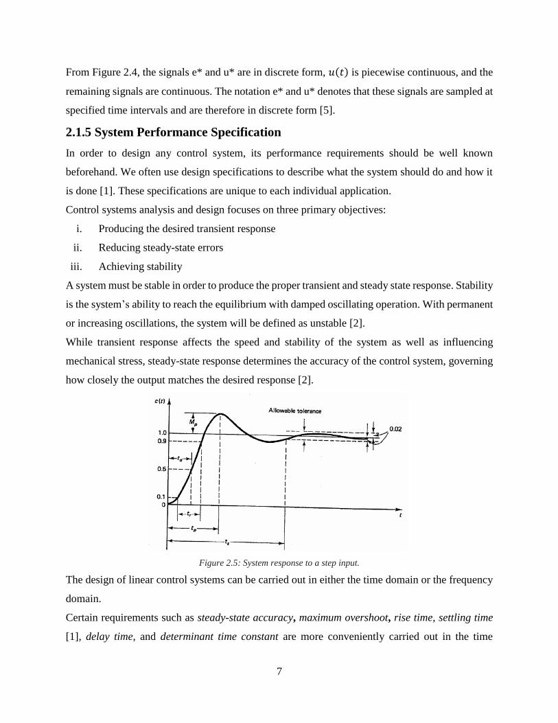
Figure 2.5: System response to a step input.
The design of linear control systems can be carried out in either the time domain or the frequency
domain.
Certain requirements such as steady-state accuracy, maximum overshoot, rise time, settling time
[1], delay time, and determinant time constant are more conveniently carried out in the time

8
domain and often specified with respect to a step input. A ramp or parabolic input could also be
applied in the case of steady state accuracy measurement.
Frequency-domain specifications include gain margin, phase margin and resonant peak amplitude
(Mr) which indicate relative stability. Others include bandwidth, cutoff rate and resonant
frequency.
Transient response specifications, see Figure 2.5, include:
Delay time (td) - the time required for the response to reach half the final value the very
first time.
Rise time (tr) - the time required for the response to rise from 10% to 90%, 5% to 95%, or
0% to 100% of its final value.
Peak time (tp) - the peak time is the time required for the response to reach the first peak of
the overshoot.
Maximum overshoot (Mp) - the maximum peak value of the response curve measured from
unity.
Maximum percent overshoot = 𝐶(𝑡𝑝)−𝐶(∞)
𝐶(∞)× 100 (2.1)
Settling time (ts) - the time required for the response curve to reach and stay within a range
about the final value of a size specified as an absolute percentage of the final value, usually
±2% or ±5%.
2.2 PID Controller
2.2.1 Introduction
Modifying a system to reshape its root locus in order to improve system performance is called
compensation or stabilization [5]. Considering that the transfer function of a system is difficult to
modify, it is necessary to introduce an appropriate compensating block if appreciable control of
the system is to be realized.
A satisfactorily compensated system should:
be stable
have a satisfactory transient response
have a large enough gain to ensure that the steady-state error does not exceed the specified
maximum.

9
2.2.2 Types of Controllers
Controller configuration and type must be chosen so that it will satisfy all the design specifications
with proper selection of its elements.
One of the best-known controllers used in practice is the PID controller, where the letters stand for
proportional, integral, and derivative.
The static behavior (gain) and the dynamic characteristics (time lag, dead time, reset time etc.) of
a process to be controlled have a significant influence on the structuring and design of the
controller and on the selection of the dimensions of its static (P component) and its dynamic
(I and D components) parameters. Precise knowledge of the type and characteristic data of the
process to be controlled is therefore essential for good control.
P Controller
This is the most simple and easy to implement controller and is mostly used in first order processes
with single energy storage to stabilize an unstable process. The main usage of this controller is to
decrease the steady state error of the system. As the proportional gain factor K increases, the steady
state error of the system decreases. However, despite the reduction, proportional control can never
manage to eliminate the steady state error of the system. As we increase the proportional gain, it
provides smaller amplitude and phase margin, faster dynamics that satisfy wider frequency band
and larger sensitivity to noise. We can use this controller only when a system is tolerable to a
constant steady state error. In addition, it can be easily concluded that applying P controller
decreases the rise time and after a certain value of reduction on the steady state error, increasing
K only leads to overshoot of the system response. This controller also directly amplifies process
noise.
The control action for a P controller is proportional to the error and this can be expressed as:
𝑢(𝑡) = 𝐾𝑝𝑒(𝑡) (2.2)
Where 𝐾𝑝is the proportional gain constant.
PI Controller
PI controllers are mainly used to eliminate the steady state error resulting from P controller.
However, in terms of the speed of the response and overall stability of the system, it has a negative
impact. This controller is mostly used in areas where speed of the system is not an issue. Since PI
controller has no ability to predict the future errors of the system it cannot decrease the rise time
and eliminate the oscillations. If applied, any amount of I guarantees set point overshoot.

10
The transfer function of the PI controller is described by the expression:
𝐺𝑐(𝑠) = 𝐾𝑝 +𝐾𝑖
𝑠 (2.3)
And the signal applied to the process is given in time domain by,
𝑢(𝑡) = 𝐾𝑝𝑒(𝑡) + 𝐾𝑖 ∫ 𝑒(𝑡)𝑑𝑡𝑡
0 (2.4)
A properly designed PI controller has the following effects on a given control system:
Improving damping and reducing maximum overshoot.
Increasing rise time and decreasing BW.
Improving gain margin, phase margin, and Mr.
Filtering out high-frequency noise.
PD Controller
The aim of using PD controller is to increase the stability of the system by improving control since
it has an ability to predict the future error of the system response. In order to avoid effects of the
sudden change in the value of the error signal, the derivative is taken from the output response of
the system variable instead of the error signal. Therefore, D mode is designed to be proportional
to the change of the output variable to prevent the sudden changes occurring in the control output
resulting from sudden changes in the error signal. In addition, D directly amplifies process noise
and therefore D-only control is not used.
A series proportional-derivative (PD) controller can be represented using the transfer function,
𝐺𝑐(𝑠) + 𝐾𝑝 + 𝐾𝑑𝑠 (2.5)
So that the control signal applied to the process, in time domain, is given by,
𝑢(𝑡) = 𝐾𝑝𝑒(𝑡) + 𝐾𝑑𝑑𝑒(𝑡)
𝑑𝑡 (2.6)
Though it is not effective with lightly damped or initially unstable systems, a properly designed
PD controller can affect the performance of a control system in the following ways [1, 10].
Improving damping and reducing maximum overshoot.
Reducing rise time and settling time but increasing BW.
Improving GM, PM, and Mr.
Possibly accentuating noise at higher frequencies since differentiation of a signal amplifies
noise and thus this term in the controller is highly sensitive to noise in the error term.
11
PID Controller
More than half of the industrial controllers in use today utilize PID or modified PID control
schemes [6]. The usefulness of PID controllers lie in their general applicability to most control
systems.
For instance, when the mathematical model of the plant is not known and therefore analytical
design methods cannot be used, PID controls prove to be most useful [6].
PID controller has the optimum control dynamics including zero steady state error, fast response
(short rise time), no oscillations and higher stability. The necessity of using a derivative gain
component in addition to the PI controller is to eliminate the overshoot and the oscillations
occurring in the output response of the system. One of the main advantages of the PID controller
is that it can be used with higher order processes including more than single energy storage.
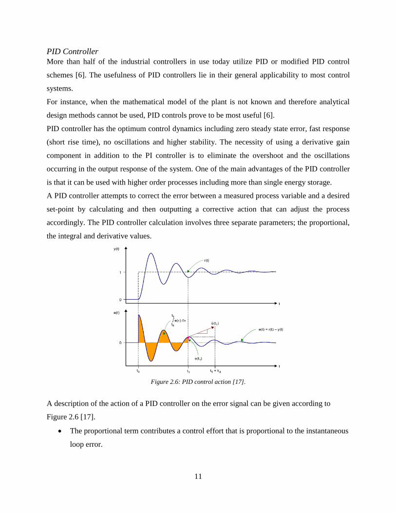
A PID controller attempts to correct the error between a measured process variable and a desired
set-point by calculating and then outputting a corrective action that can adjust the process
accordingly. The PID controller calculation involves three separate parameters; the proportional,
the integral and derivative values.
Figure 2.6: PID control action [17].
A description of the action of a PID controller on the error signal can be given according to
Figure 2.6 [17].
The proportional term contributes a control effort that is proportional to the instantaneous
loop error.
12
The output of the integral path is the accumulated error history: the shaded area in the
lower plot.
The contribution of the derivative path is proportional to the rate of change of the loop
error. Derivative gain fixes the time interval over which a tangential line to the error curve
is projected into the future. It thus provides a predictive feature for PID control.
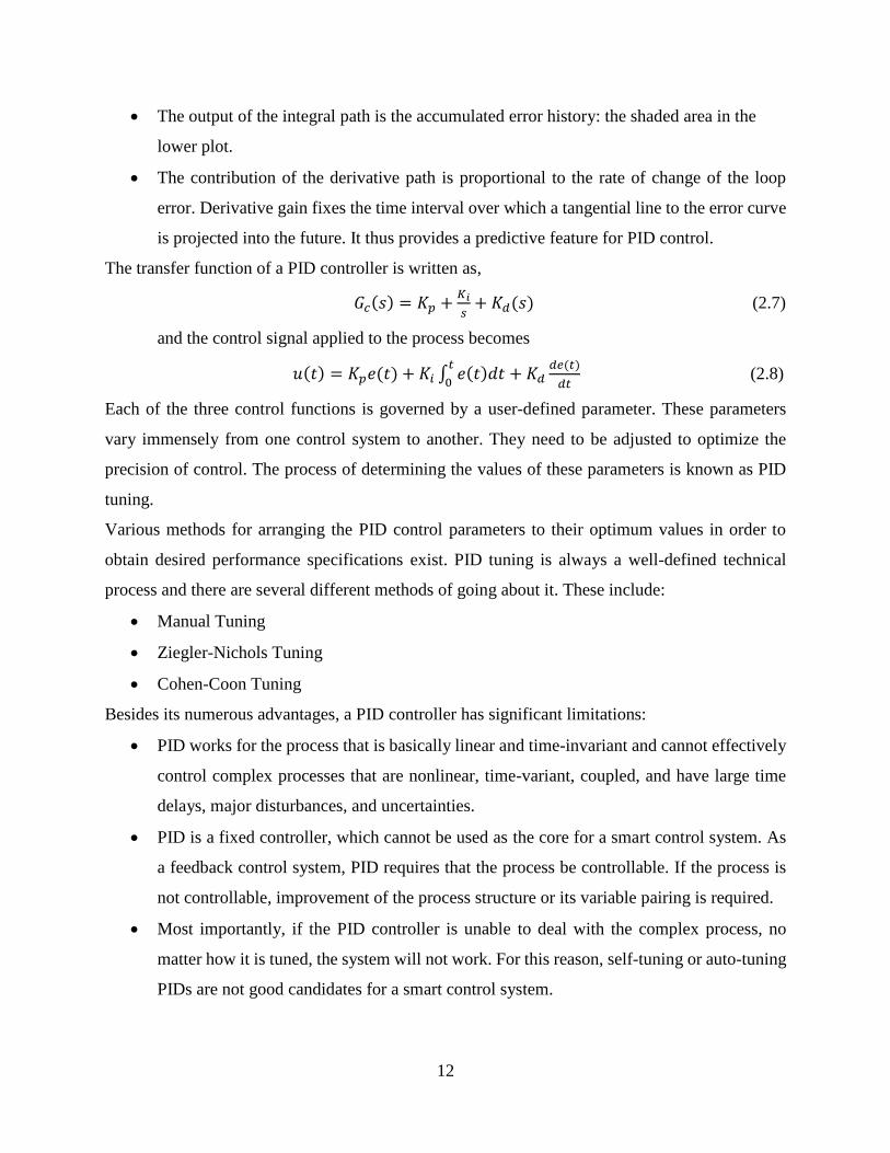
The transfer function of a PID controller is written as,
𝐺𝑐(𝑠) = 𝐾𝑝 +𝐾𝑖
𝑠+ 𝐾𝑑(𝑠) (2.7)
and the control signal applied to the process becomes
𝑢(𝑡) = 𝐾𝑝𝑒(𝑡) + 𝐾𝑖 ∫ 𝑒(𝑡)𝑑𝑡𝑡
0+ 𝐾𝑑
𝑑𝑒(𝑡)
𝑑𝑡 (2.8)
Each of the three control functions is governed by a user-defined parameter. These parameters
vary immensely from one control system to another. They need to be adjusted to optimize the
precision of control. The process of determining the values of these parameters is known as PID
tuning.
Various methods for arranging the PID control parameters to their optimum values in order to
obtain desired performance specifications exist. PID tuning is always a well-defined technical
process and there are several different methods of going about it. These include:
Manual Tuning
Ziegler-Nichols Tuning
Cohen-Coon Tuning
Besides its numerous advantages, a PID controller has significant limitations:
PID works for the process that is basically linear and time-invariant and cannot effectively
control complex processes that are nonlinear, time-variant, coupled, and have large time
delays, major disturbances, and uncertainties.
PID is a fixed controller, which cannot be used as the core for a smart control system. As
a feedback control system, PID requires that the process be controllable. If the process is
not controllable, improvement of the process structure or its variable pairing is required.
Most importantly, if the PID controller is unable to deal with the complex process, no
matter how it is tuned, the system will not work. For this reason, self-tuning or auto-tuning
PIDs are not good candidates for a smart control system.

13
2.3 Programmable Logic Controllers
Figure 2.7: Siemens SIMATIC S7-200 (CPU 224) PLC
Programmable logic controllers (PLCs) are members of the computer family which are used to
implement control functions involving storage of instructions, data manipulation and
communication in order to control industrial machines and processes [7, 8]. Figure 2.7 illustrates
a diagram of a PLC.
PLCs can be regarded as industrial computers with specially designed architecture in both their
central processing units and their interfacing circuitry to field devices [7].
2.3.1 PLC Architecture
The internal architecture of a PLC is as shown in Figure 2.8.
Figure 2.8: Typical architecture of a PLC [8].

14
Central Processing Unit
At the very basic, the internal architecture of a PLC consists of a central processing unit (CPU)
containing the system microprocessor, memory and input/output circuitry. The CPU is supplied
with a clock which determines the operating speed of the PLC and provides the timing and
synchronization for all elements in the system.
The information within the PLC is carried by means of digital signals which flow along internal
paths called buses.
Memory system
This is the area in the PLC where all of the sequences of instructions, or programs, are stored and executed
by the processor to provide the desired control of field devices [7]. The memory sections that contain the
control programs can be reprogrammed to adapt to any changes in process control requirements.
I/O Interfaces
An I/O module is a plug-in–type assembly containing circuitry that communicates between a PLC
and field devices. These devices could be transmitting and/or accepting digital or analog signals.
(a) (b)
Figure 2.9: (a) the EM222 digital I/O and
(b) the EM235 analog I/O expansion modules
The power supply
The system power supply provides internal DC voltages to the system components (processor,
memory, and input/output interfaces).
Figure 2.10: Power supply unit (with PLC and I/O interfaces)
15
The power supply is characterized by a maximum amount of current that it can provide at a given
voltage level, depending on the type of power supply.
An understanding of PLC product ranges and their characteristics (I/O count, memory size,
programming language and software functions) will allow a user to properly identify the controller
that will satisfy a particular application [7].
2.3.2 PLC System and Principles of Operation [7, 8]
During its operation, the CPU completes three processes:
Reads (accepts) the input data from the field devices via the input interfaces.
Executes (performs) the control program stored in the memory system.
Writes (updates) the output devices via the output interfaces.
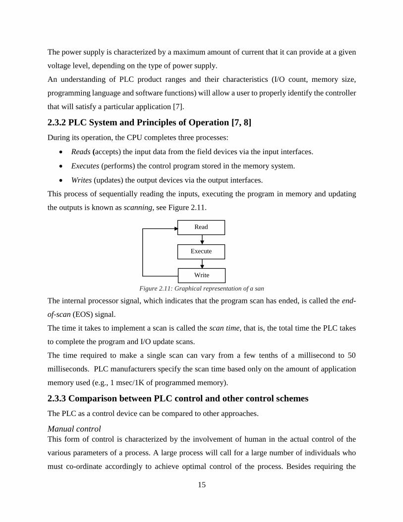
This process of sequentially reading the inputs, executing the program in memory and updating
the outputs is known as scanning, see Figure 2.11.
Figure 2.11: Graphical representation of a san
The internal processor signal, which indicates that the program scan has ended, is called the end-
of-scan (EOS) signal.
The time it takes to implement a scan is called the scan time, that is, the total time the PLC takes
to complete the program and I/O update scans.
The time required to make a single scan can vary from a few tenths of a millisecond to 50
milliseconds. PLC manufacturers specify the scan time based only on the amount of application
memory used (e.g., 1 msec/1K of programmed memory).
2.3.3 Comparison between PLC control and other control schemes
The PLC as a control device can be compared to other approaches.
Manual control
This form of control is characterized by the involvement of human in the actual control of the
various parameters of a process. A large process will call for a large number of individuals who
must co-ordinate accordingly to achieve optimal control of the process. Besides requiring the
Read
Write
Execute

16
presence of human to start, run and stop a process, this control method is tedious, repetitive and
prone to numerous errors and downtimes hence the need for automatic control.
However, some form of manual control is incorporated in automatic control systems to facilitate
override in case of failure. This is usually a security and safety requirement in the design of
automatic control systems.
Relay Logic
Large bundles of wires and interconnections associated with using relays in the implementation of
a large complex system result in the control panel occupying a large space. It also renders
troubleshooting and maintenance quite difficult.
If system requirements call for flexibility or future growth, a programmable controller brings
returns that outweigh any initial cost advantage of a relay control system.
The extremely short cycle (scan) time of a PLC allows the productivity of machines that were
previously under electromechanical control to increase considerably.
Computer Control
Even though the architecture of a PLC’s CPU is basically the same as that of a general purpose
computer, some important characteristics set them apart.
Unlike computers, PLCs are specifically designed to survive the harsh conditions of the
industrial environment such as electrical noise, electromagnetic interference, mechanical
vibration and noncondensing humidity.
Whereas computers are complex computing machines capable of executing several
programs or tasks simultaneously and in any order, so far the standard PLC still executes
a single program in an orderly, sequential fashion from first to last instruction. On the other
hand, the hardware and software for PLC is designed for easy use by electricians and
technicians.
2.3.4 PLC Programming
Programming languages allow the user to enter a control program into a PLC using an established
syntax.
The IEC 1131-3 standard defines three graphical languages and two text-based languages for use
in PLC programming. The graphical languages use symbols to program control instructions, while
the text-based languages use character strings to program instructions.
17
Graphical languages
i. Ladder diagrams (LD) - uses a standardized set of ladder programming symbols to
implement control functions.
ii. Function Block Diagram (FBD) - a graphical language that allows the user to program
elements in such a way that they appear to be wired together like electrical circuits.
iii. Sequential Functional Chart (SFC) - a graphical language that provides a diagrammatic
representation of control sequences in a program.
Text-based languages
i. Instruction list (IL) - a low-level language similar to the machine or assembly language
used with microprocessors.
ii. Structured text (ST) - a high-level language that allows structured programming, meaning
that many complex tasks can be broken down into smaller ones.
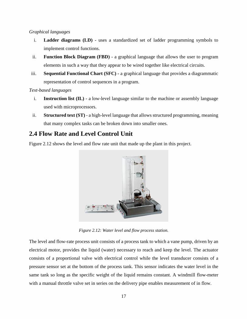
2.4 Flow Rate and Level Control Unit
Figure 2.12 shows the level and flow rate unit that made up the plant in this project.
Figure 2.12: Water level and flow process station.
The level and flow-rate process unit consists of a process tank to which a vane pump, driven by an
electrical motor, provides the liquid (water) necessary to reach and keep the level. The actuator
consists of a proportional valve with electrical control while the level transducer consists of a
pressure sensor set at the bottom of the process tank. This sensor indicates the water level in the
same tank so long as the specific weight of the liquid remains constant. A windmill flow-meter
with a manual throttle valve set in series on the delivery pipe enables measurement of in flow.

18
(a) (b)
Figure 2.13: (a) proportional valve and (b) discharge solenoid valve
At the bottom of the process tank are a solenoid valve for automatic control of outflow of water
from the process tank. Manual control of outflow is enabled by a manual valve connected in
parallel with the solenoid valve.
Beneath the process tank is a reservoir tank that provides water to be fed to the process tank as
well as serving as a collector. This reservoir tank is fitted with a manual throttle valve that enables
the setting of the “load” and its variations.
The transparent process tank has a metric reference line for level reading. The level range is from
0 to 500 mm. The inner volume between level 0 and 500 mm is of 5 liters and this is considered
the reference in the flow measurements.
The complete system includes a unit containing a power amplifier and signal conditioning modules
for level and flow transducers.
2.5 Fluid Dynamics
2.5.1 Introduction
Fluid dynamics is a study of the concepts necessary to analyze fluids in motion.
Fluid Flow
The basic approach of any given flow measurement technique depends on the flowing medium
and nature of the flow.
The flow of fluids can be classified, according to the magnitude of the Reynolds number, into:
Steady (laminar) flow - velocity, pressure and cross-section may differ from point to point
but do not change with time.
Unsteady (turbulent) flow - velocity, pressure and cross-section change with time.
Practically, there is always slight variations in velocity and pressure, but if the average
values are constant, the flow is considered steady.
If the Reynolds number is greater than about 3000 to 4000, then the flow is turbulent. The flow is
laminar if the Reynolds number is less than about 2000 [6].
19
Compression
All fluids (even water) are compressible, that is, their density will change as pressure changes.
Under steady conditions, and provided that the changes in pressure are small, it is usually possible
to simplify analysis of the flow by assuming it is incompressible and has constant density.
2.5.2 Flow Rate
Mass Flow Rate
This is a measure of the rate of accumulation of mass and is expressed as:
Mass flow rate, m = 𝑚𝑎𝑠𝑠 𝑜𝑓 𝑓𝑙𝑢𝑖𝑑
𝑡𝑖𝑚𝑒 𝑡𝑎𝑘𝑒𝑛 𝑡𝑜 𝑎𝑐𝑢𝑚𝑢𝑙𝑎𝑡𝑒 𝑡ℎ𝑒 𝑚𝑎𝑠𝑠 (2.9)
Volume flow rate (Discharge)
This is the volume of fluid flowing per unit time. Multiplying this by the density of the fluid gives
us the mass flow rate.
Discharge, Q = 𝑣𝑜𝑙𝑢𝑚𝑒 𝑜𝑓 𝑓𝑙𝑢𝑖𝑑
𝑡𝑖𝑚𝑒
= 𝑚𝑎𝑠𝑠 𝑜𝑓 𝑓𝑙𝑢𝑖𝑑
𝑑𝑒𝑛𝑠𝑖𝑡𝑦×𝑡𝑖𝑚𝑒
= 𝑚𝑎𝑠𝑠 𝑓𝑙𝑜𝑤 𝑟𝑎𝑡𝑒
𝑑𝑒𝑛𝑠𝑖𝑡𝑦 (2.10)
Energy losses due to friction
In a real pipe line there are energy losses due to friction. These losses can be very significant and
therefore must be taken into account.
Taking total head (total energy per unit weight) to be constant and considering energy
conservation, allowing for an amount of energy to be lost due to friction will change the total head.
The energy loss can be represented by the symbol ℎ𝑓 such that head loss due to friction can be
shown by Bernoulli’s equation of the form;
𝑃1
𝜌𝑔+
𝑣12
2𝑔+ 𝑧1 =
𝑃2
𝜌𝑔+
𝑣22
2𝑔+ 𝑧2 + ℎ𝑓 (2.11)
In order to account for the deviation of actual velocity from theoretical velocity due to friction
losses, the coefficient of velocity is used to correct the theoretical velocity, that is:
𝑣𝑎𝑐𝑡𝑢𝑎𝑙 = 𝐶𝑣𝑣𝑡ℎ𝑒𝑜𝑟𝑒𝑡𝑖𝑎𝑙 (2.12)
Each orifice has its own coefficient of velocity which usually lies in the range (0.97 - 0.99).

20
CHAPTER 3: METHODOLOGY AND DESIGN
3.1 Overview
3.1.1 Design Stages [1, 3, 5]
The design and implementation of any control system involves several steps that are followed in
order to realize the physical system. Figure 3.1 shows the various steps that were followed in this
project.
Figure 3.1: Design steps
3.1.2 Performance Specifications
The preset level of water in the tank was obtained from a potentiometer calibrated between zero
and 10V to represent the full range of the tank height (0mm to 500mm).
The signal from the level transducer was fed back to the PLC and compared with the set point
value to obtain the actuating signal and consequently, the PID algorithm was implemented. The
actuating device (proportional valve) was then supposed to be driven appropriately so that the
actual water level tracks the desired level to required specifications even in the event unforeseen
disturbances occur.
Establish Design Specifications
Divide process into individual components and describe
each sub-process
Model Behavior of Plant and System Components to Obtain
System Transfer Function
Define Strategy for Performance Analysis using Transfer
Function for both Hardware and Software
Develop a Testing Strategy (for HW and SW)
Design, Generate and Simulate/Test Software
Implement and Test Actual System

21
Sensing Sub-process
Actuation Sub-process Controller Sub-process
𝑅(𝑠)
Input Sub-process
Given that such a process is considered to be slow, the basic performance specifications for this
system were defined as:
Settling time < 45 seconds
Overshoot < 1%;
Steady state error < 2%
Damping ratio = 0.7
3.2 Process Modelling
3.2.1 Introduction
After defining the process to be controlled, the next step was to identify groups of related
components in order to break down the process into smaller less complicated sub processes.
Figure 3.2a: General block diagram of a process control system
Figure 3.2b Configuration diagram for water level control
𝐶(𝑠) 𝑅(𝑠)
-
+
Controller
𝐺𝑐(𝑠)
Potentiometer Process
Pump
A
D
C
PLC with
arithmetic
and data
manipulation
instructions
plus PID
algorithm
D
A
C
Discharge
Solenoid
Proportional
Valve
Level Sensor
Flow Rate Sensor
Process
𝐺𝑝(𝑠)
Actuator
𝐺𝑎(𝑠)
Transducer
𝐻(𝑠)
𝐶(𝑠)
Power Supply
22
3.2.2 Description of Individual Components
The decision on what type of controlling device(s), sensors and actuating devices are essential in
the implementation of a control system is a crucial step in any system design.
However, the station for this project was already fabricated and so the choice of sensors, actuators,
power supply or PLC type was already restricted. The controller type was also specified to be PID.
3.2.3 Dynamic Behavior of Process
In order to understand and control complex systems, we must obtain their quantitative
mathematical models by analyzing the relationships between the system variables and employing
Laplace transform or other mathematical tools [15]. A set of linear differential equations were
formulated to obtain model transfer functions that described the physical system.
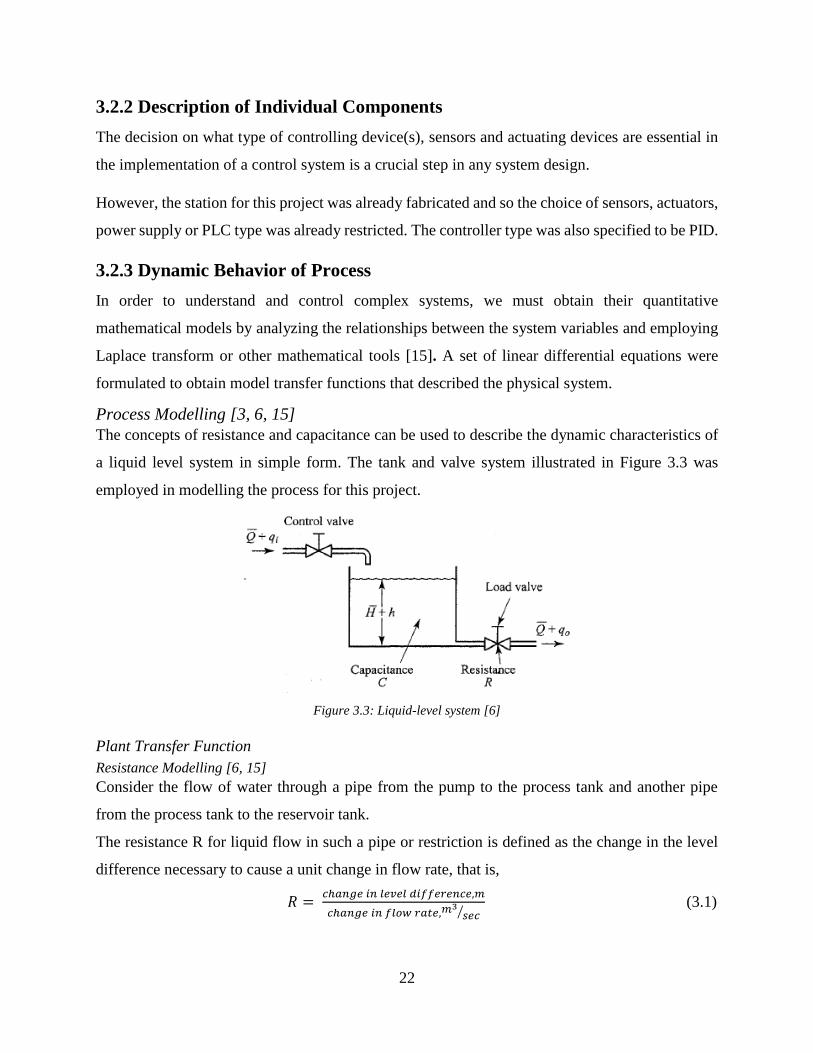
Process Modelling [3, 6, 15]
The concepts of resistance and capacitance can be used to describe the dynamic characteristics of
a liquid level system in simple form. The tank and valve system illustrated in Figure 3.3 was
employed in modelling the process for this project.
Figure 3.3: Liquid-level system [6]
Plant Transfer Function
Resistance Modelling [6, 15]
Consider the flow of water through a pipe from the pump to the process tank and another pipe
from the process tank to the reservoir tank.
The resistance R for liquid flow in such a pipe or restriction is defined as the change in the level
difference necessary to cause a unit change in flow rate, that is,
𝑅 = 𝑐ℎ𝑎𝑛𝑔𝑒 𝑖𝑛 𝑙𝑒𝑣𝑒𝑙 𝑑𝑖𝑓𝑓𝑒𝑟𝑒𝑛𝑐𝑒,𝑚
𝑐ℎ𝑎𝑛𝑔𝑒 𝑖𝑛 𝑓𝑙𝑜𝑤 𝑟𝑎𝑡𝑒,𝑚3
𝑠𝑒𝑐⁄ (3.1)

23
Since the flow through this restriction (load valve in the side of the tank) is assumed to be laminar,
the relationship between the steady-state flow rate and steady-state head at the level of the
restriction is given by
𝑄 = 𝐾𝐻 (3.2)
Where Q = steady-state liquid flow rate, m3/sec
K = coefficient, m2/sec
H = steady-state head, m
The resistance Rl is obtained as,
𝑅𝑙 =𝑑𝐻
𝑑𝑄=
𝐻
𝑄 (3.3)
The laminar flow resistance is thus constant and is analogous to the electrical resistance. It is
however worth noting that the value of K in Equation 3.2 depends on the flow coefficient and the
area of restriction.
Capacitance Modelling [6, 14]
The capacitance C of a tank is defined to be the change in quantity of stored liquid necessary to
cause a unit change in the potential (head). It can given by the expression,
𝐶 = 𝑐ℎ𝑎𝑛𝑔𝑒 𝑖𝑛 𝑙𝑖𝑞𝑢𝑖𝑑 𝑠𝑡𝑜𝑟𝑒𝑑,𝑚3
𝑐ℎ𝑎𝑛𝑔𝑒 𝑖𝑛 ℎ𝑒𝑎𝑑,𝑚 (3.4)
It can be noted the capacitance of the tank is equal to its cross-sectional area and thus 𝐶 can be
substituted with 𝐴. If this is constant, the capacitance is constant for any head.
Having modelled the resistance and capacitance of the tank, the overall plant transfer function can
be obtained using the values obtained.
The variables in Figure 3.3 can be defined as follows:
�̅� = steady state flow rate (before any change has occurred), m3/sec
𝑞𝑖 = small deviation of inflow rate from its steady state value, m3/sec
𝑞𝑜 = small deviation of outflow rate from its steady state value, m3/sec
𝑞𝑛 = Adh = net tank rate of flow
�̅� = steady state head (before any change has occurred), m
h = small deviation of head from its steady state value, m
All assumptions holding, the differential equation of this system can be obtained. Since the inflow
minus outflow during the small time interval dt is equal to the additional amount stored in the tank,
we find that,

24
𝐴𝑑ℎ = (𝑞𝑖 − 𝑞𝑜)𝑑𝑡 = 𝑞𝑛𝑑𝑡 (3.5)
From the definition of resistance, the relationship between 𝑞𝑜 and h is given by,
𝑞𝑜 = ℎ
𝑅 (3.6)
So that the differential equation for this system for a constant value of R becomes
𝑅𝐴𝑑ℎ
𝑑𝑡+ ℎ = 𝑅𝑞𝑖 (3.7)
Note that RA is the time constant of the system. Taking the Laplace transforms of both sides of
Equation 3.7 assuming zero initial condition, we obtain,
(𝑅𝐴𝑠 + 1) 𝐻(𝑠) = 𝑅𝑄𝑖(𝑠) (3.8)
If 𝑞𝑖 is considered the input and h the output, the transfer function of the system is,
𝐻(𝑠)
𝑄𝑖(𝑠)=
𝑅
𝑅𝐴𝑠 + 1
The actuator was considered to be in cascade with the plant and therefore the overall transfer
fuction for the process set up was epressed as:
𝐺𝑝(𝑠) =𝐾𝑣𝑅
𝑅𝐴𝑠+1 (3.9)
Where 𝐾𝑣 is flow coefficient (a factor of the actuating valve).
Plant Time Constant
Time constant of the tank,𝜏, may be defined either as the time to reach 63.2% of its steady state
(final value) or the time to reach the final value if the initial slope (rate of change) could be
maintained. The larger the time constant, the more the output lags behind the input.
The open loop response of the plant to a step increase in the pump drive voltage was required since
it would provide the system’s dominant time constant and form the basis for choosing the
controller.
There are several methods for estimating the time constant of a tank level system, that is:
i. Initial tank level free response
ii. Head versus flow rate relationship.
Initial tank level free response method was preferred because it is easy to implement and not prone
to errors compared to the second method.
With knowledge of the tank geometry and maximum inflow rate the tank time constant could be
calculated from the fill time which can be obtained by:
𝑇𝑓𝑖𝑙𝑙 =𝑄
𝐹
25
Where:
𝑇𝑓𝑖𝑙𝑙 – Tank fill time.
Q – Volume of tank between lower and upper limits
F – Maximum flow rate
Direct application of this relation resulted in:
𝑇𝑓𝑖𝑙𝑙 =5 𝑙𝑖𝑡𝑟𝑒𝑠
5 𝑙 𝑚𝑖𝑛⁄= 1 min = 60 𝑠𝑒𝑐𝑜𝑛𝑑𝑠
In order to experimentally apply this method to determine the time constant of the tank system,
discharge valves were closed and the pump was turned on. The time for water level to rise from
0mm to 500mm at maximum inflow rate (5.10 l/min) was measured using PLC timers and recorded
as shown in Table 3.1.
Table 3.1: Plant time constant
Index 01 02 03 04 05 06 07 Average
Time (s) 63.8 62.7 62.4 63.2 62.6 62.8 61.9 62.77
In order to determine the time it took to empty the tank, tank holdup method for free response was
applied. First, the tank was filled to maximum level with all valves closed. The solenoid valve was
then opened by applying 24Vdc to energize it. The time taken by the water level to drop to 0mm
was measured and recorded as illustrated in Table 3.2.
Table 3.2: Discharge time
Index 01 02 03 04 05 06 07 Average
Time (s) 112.4 111.0 112.2 108.8 109.1 109.8 108.0 110.19
In order to account for flow dynamics, the time constant, 𝜏 = 𝑅𝐴 , was taken to be 62.77 seconds.
Since we have that,
𝐴 = 10 ∗ 10 = 100𝑐𝑚2
Then,
𝑅 =𝜏
𝐴=
62.77
0.01= 6277 𝑠𝑚−2 (3.10)
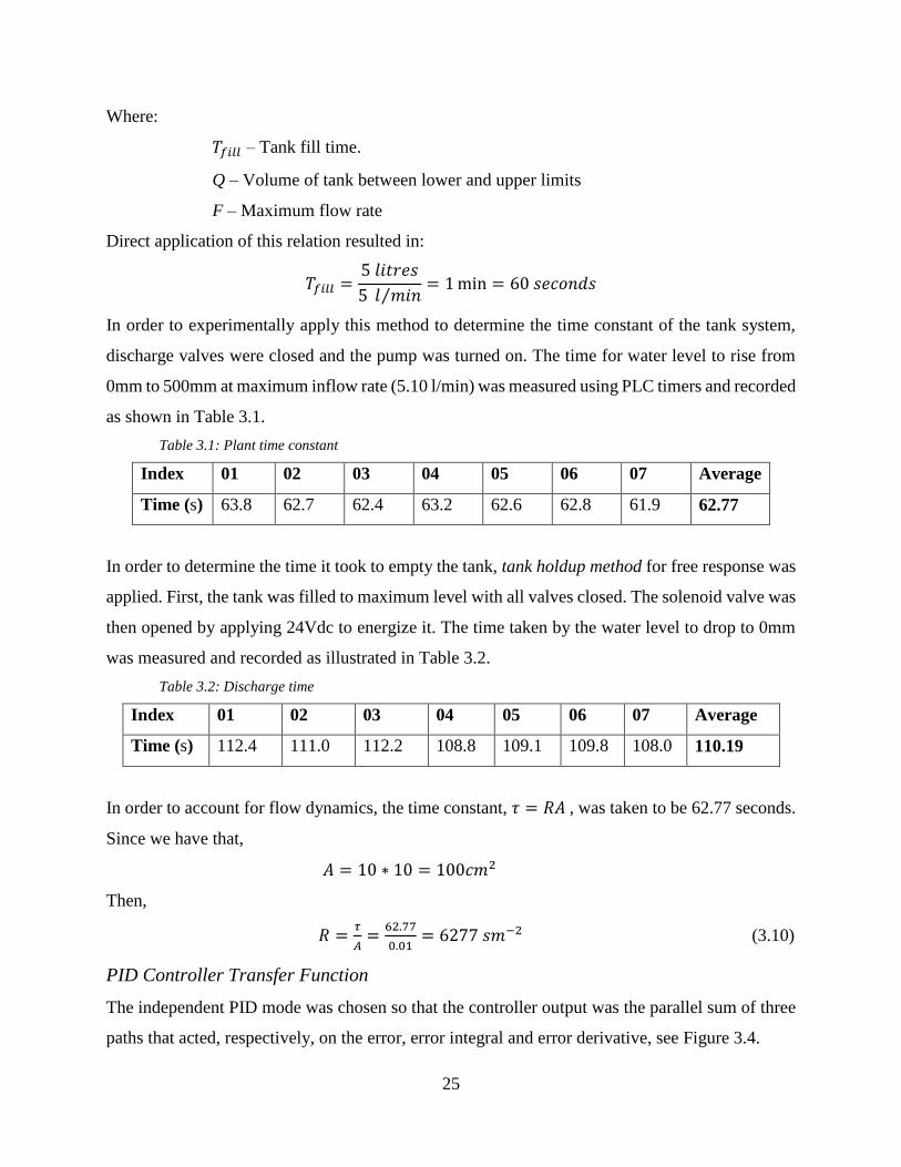
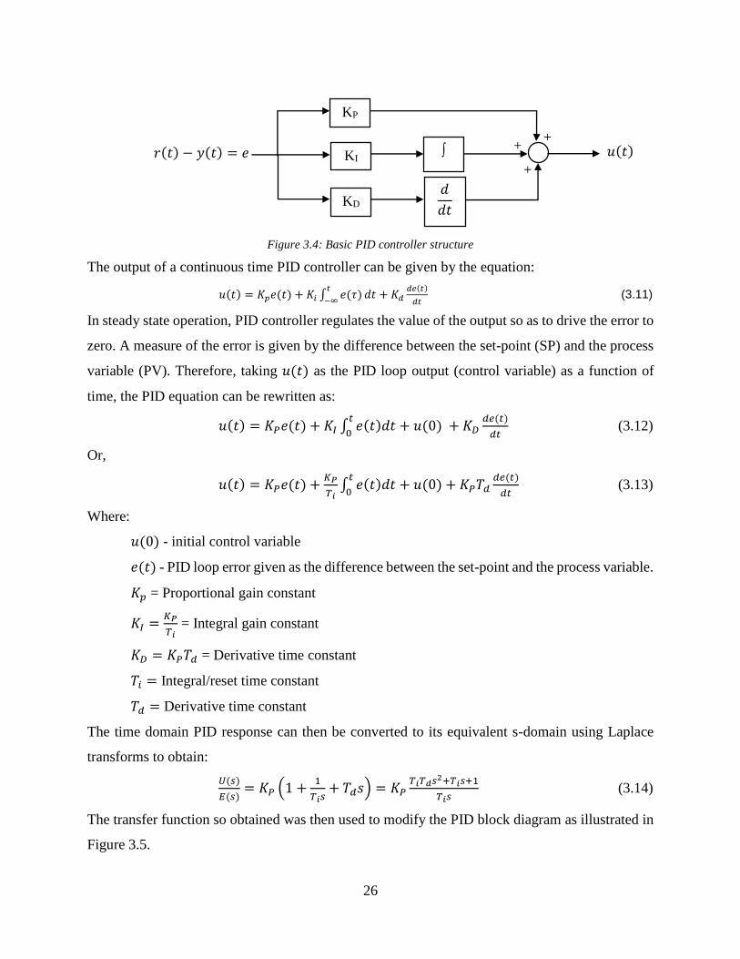
PID Controller Transfer Function
The independent PID mode was chosen so that the controller output was the parallel sum of three
paths that acted, respectively, on the error, error integral and error derivative, see Figure 3.4.
26
Figure 3.4: Basic PID controller structure
The output of a continuous time PID controller can be given by the equation:
𝑢(𝑡) = 𝐾𝑝𝑒(𝑡) + 𝐾𝑖 ∫ 𝑒(𝜏)𝑡
−∞𝑑𝑡 + 𝐾𝑑
𝑑𝑒(𝑡)
𝑑𝑡 (3.11)
In steady state operation, PID controller regulates the value of the output so as to drive the error to
zero. A measure of the error is given by the difference between the set-point (SP) and the process
variable (PV). Therefore, taking 𝑢(𝑡) as the PID loop output (control variable) as a function of
time, the PID equation can be rewritten as:
𝑢(𝑡) = 𝐾𝑃𝑒(𝑡) + 𝐾𝐼 ∫ 𝑒(𝑡)𝑑𝑡𝑡
0+ 𝑢(0) + 𝐾𝐷
𝑑𝑒(𝑡)
𝑑𝑡 (3.12)
Or,
𝑢(𝑡) = 𝐾𝑃𝑒(𝑡) +𝐾𝑃
𝑇𝑖∫ 𝑒(𝑡)𝑑𝑡 + 𝑢(0)
𝑡
0+ 𝐾𝑃𝑇𝑑
𝑑𝑒(𝑡)
𝑑𝑡 (3.13)
Where:
𝑢(0) - initial control variable
𝑒(𝑡) - PID loop error given as the difference between the set-point and the process variable.
𝐾𝑝 = Proportional gain constant
𝐾𝐼 =𝐾𝑃
𝑇𝑖 = Integral gain constant
𝐾𝐷 = 𝐾𝑃𝑇𝑑 = Derivative time constant
𝑇𝑖 = Integral/reset time constant
𝑇𝑑 = Derivative time constant
The time domain PID response can then be converted to its equivalent s-domain using Laplace
transforms to obtain:
𝑈(𝑠)
𝐸(𝑠)= 𝐾𝑃 (1 +
1
𝑇𝑖𝑠+ 𝑇𝑑𝑠) = 𝐾𝑃
𝑇𝑖𝑇𝑑𝑠2+𝑇𝑖𝑠+1
𝑇𝑖𝑠 (3.14)
The transfer function so obtained was then used to modify the PID block diagram as illustrated in
Figure 3.5.
𝑢(𝑡)
𝑟(𝑡) − 𝑦(𝑡) = 𝑒
+
+ +
KP
∫
𝑑
𝑑𝑡 KD
KI

27
Figure 3.5: Reduced Basic PID controller structure
Where 𝐾𝑐 is known as the controller gain.
Siemens S7-200 CPU 224 PLC PID Loop Algorithm
As a result of the repetitive nature of the digital computer solution, a simplification of Equation
3.13 that must be solved at any sample time can be made.
𝑢𝑁 = 𝐾𝑐 ∗ 𝑒𝑛 + 𝐾𝑐 ∗𝑇𝑠
𝑇𝑖∗ 𝑒𝑛 + 𝑢𝑖𝑛𝑖𝑡𝑖𝑎𝑙 + 𝐾𝑐 ∗
𝑇𝑑
𝑇𝑠∗ (𝑒𝑛 − 𝑒𝑛−1) (3.15)
The integral sum or bias 𝑢𝑖𝑛𝑖𝑡𝑖𝑎𝑙 is the running sum of all previous values of the integral term.
After each calculation of the current integral term, the bias is updated with the value of this integral
term which might be adjusted or clamped to conform to the variable and range requirement of the
PLC. The initial value of the bias is typically set to the output value 𝑢𝑖𝑛𝑖𝑡𝑖𝑎𝑙 just prior to the first
loop output calculation.
A simplified form of the PID controller can be written as:
𝑢𝑡𝑜𝑡𝑎𝑙(𝑛) = 𝑢𝑝(𝑛) + 𝑢𝑖(𝑛) + 𝑢𝑑(𝑛)
Since 𝑒𝑛 = 𝑆𝑃𝑛 − 𝑃𝑉𝑛 and 𝑒𝑛−1 = 𝑆𝑃𝑛−1 − 𝑃𝑉𝑛−1 , the derivative term of Equation 3.15 can be
expressed in the form
𝑢𝑑(𝑛) = 𝐾𝑐 ∗𝑇𝑑
𝑇𝑠∗ ((𝑆𝑃𝑛 − 𝑃𝑉𝑛) − (𝑆𝑃𝑛−1 − 𝑃𝑉𝑛−1))
In order avoid step changes or bumps in the output due to derivative action on set point changes,
this equation is modified to assume that the set point is a constant (SPn = SPn-1). This results in the
calculation of the change in the process variable instead of the change in the error as shown:
𝑢𝑑(𝑛) = 𝐾𝑐 ∗𝑇𝑑
𝑇𝑠∗ (𝑆𝑃𝑛 − 𝑃𝑉𝑛 − 𝑆𝑃𝑛 + 𝑃𝑉𝑛−1)
Or simply
𝑢𝑑(𝑛) = 𝐾𝑐 ∗𝑇𝑑
𝑇𝑠∗ (𝑃𝑉𝑛−1 − 𝑃𝑉𝑛)
𝑈(𝑠)
+
+
+
- +
𝑃𝑣
𝑆𝑝 𝐾𝑐
1𝑇𝑖
⁄
1𝑠⁄
1
𝑇𝑑 s
28
The process variable rather than the error must be saved for use in the next calculation of the
differential term. At the time of the first sample, the value of PVn-1 is initialized to be equal to PVn.
The modified PID function thus becomes:
𝑢𝑁 = 𝐾𝑐 ∗ (𝑆𝑃𝑛 − 𝑃𝑉𝑛) + 𝐾𝑐 ∗𝑇𝑠
𝑇𝑖∗ (𝑆𝑃𝑛 − 𝑃𝑉𝑛) + 𝑢𝑖𝑛𝑖𝑡𝑖𝑎𝑙 + 𝐾𝑐 ∗
𝑇𝑑
𝑇𝑠∗ (𝑃𝑉𝑛−1 − 𝑃𝑉𝑛) (3.16)
System Transfer Function
Continuous Time Transfer Function
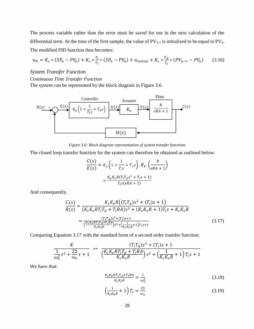
The system can be represented by the block diagram in Figure 3.6.
Figure 3.6: Block diagram representation of system transfer functions
The closed loop transfer function for the system can therefore be obtained as outlined below:
𝐶(𝑠)
𝐸(𝑠)= 𝐾𝑝 (1 +
1
𝑇𝑖𝑠+ 𝑇𝑑𝑠) . 𝐾𝑣. (
𝑅
𝑠𝑅𝐴 + 1)
=𝐾𝑝𝐾𝑣𝑅(𝑇𝑖𝑇𝑑𝑠2 + 𝑇𝑖𝑠 + 1)
𝑇𝑖𝑠(𝑠𝑅𝐴 + 1)
And consequently,
𝐶(𝑠)
𝑅(𝑠)=
𝐾𝑐𝐾𝑣𝑅((𝑇𝑖𝑇𝑑)𝑠2 + (𝑇𝑖)𝑠 + 1)
(𝐾𝑐𝐾𝑣𝑅𝑇𝑖𝑇𝑑 + 𝑇𝑖𝑅𝐴)𝑠2 + (𝐾𝑐𝐾𝑣𝑅 + 1)𝑇𝑖𝑠 + 𝐾𝑐𝐾𝑣𝑅
=(𝑇𝑖𝑇𝑑)𝑠2+(𝑇𝑖)𝑠+1
(𝐾𝑐𝐾𝑣𝑅𝑇𝑖𝑇𝑑+𝑇𝑖𝑅𝐴
𝐾𝑐𝐾𝑣𝑅)𝑠2+(
1
𝐾𝑐𝐾𝑣𝑅+1)𝑇𝑖𝑠+1
(3.17)
Comparing Equation 3.17 with the standard form of a second order transfer function;
𝐾
1𝜔𝑛
2 𝑠2 +2ℶ𝜔𝑛
𝑠 + 1 ↔
(𝑇𝑖𝑇𝑑)𝑠2 + (𝑇𝑖)𝑠 + 1
(𝐾𝑐𝐾𝑣𝑅𝑇𝑖𝑇𝑑 + 𝑇𝑖𝑅𝐴
𝐾𝑐𝐾𝑣𝑅 ) 𝑠2 + (1
𝐾𝑐𝐾𝑣𝑅 + 1) 𝑇𝑖𝑠 + 1
We have that:
𝐾𝑐𝐾𝑣𝑅𝑇𝑖𝑇𝑑+𝑇𝑖𝑅𝐴
𝐾𝑐𝐾𝑣𝑅=
1
𝜔𝑛2 (3.18)
(1
𝐾𝑐𝐾𝑣𝑅+ 1) 𝑇𝑖 =
2ℶ
𝜔𝑛 (3.19)
𝑉(𝑠) 𝑈(𝑠) 𝐸(𝑠)
Plant Actuator Controller
+
- 𝐾𝑝 (1 +
1
𝑇𝑖𝑠+ 𝑇𝑑𝑠) 𝐾𝑣
𝑅
𝑠𝑅𝐴 + 1
𝐻(𝑠)
𝑅(𝑠) 𝐶(𝑠)
29
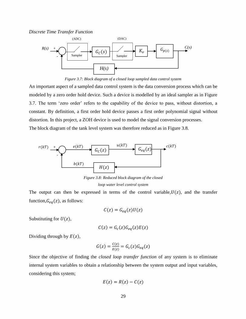
Discrete Time Transfer Function
Figure 3.7: Block diagram of a closed loop sampled data control system
An important aspect of a sampled data control system is the data conversion process which can be
modeled by a zero order hold device. Such a device is modelled by an ideal sampler as in Figure
3.7. The term ‘zero order’ refers to the capability of the device to pass, without distortion, a
constant. By definition, a first order hold device passes a first order polynomial signal without
distortion. In this project, a ZOH device is used to model the signal conversion processes.
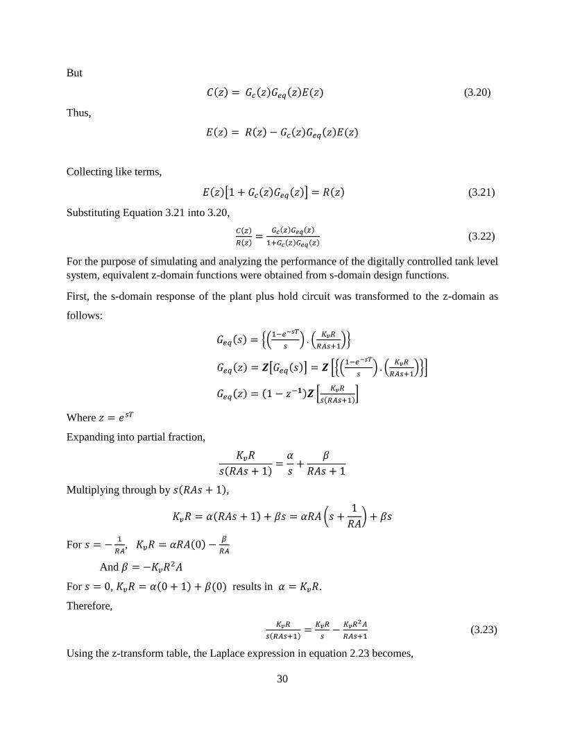
The block diagram of the tank level system was therefore reduced as in Figure 3.8.
Figure 3.8: Reduced block diagram of the closed
loop water level control system
The output can then be expressed in terms of the control variable,𝑈(𝑧), and the transfer
function,𝐺𝑒𝑞(𝑧), as follows:
𝐶(𝑧) = 𝐺𝑒𝑞(𝑧)𝑈(𝑧)
Substituting for 𝑈(𝑧),
𝐶(𝑧) = 𝐺𝑐(𝑧)𝐺𝑒𝑞(𝑧)𝐸(𝑧)
Dividing through by 𝐸(𝑧),
𝐺(𝑧) =𝐶(𝑧)
𝐸(𝑧)= 𝐺𝑐(𝑧)𝐺𝑒𝑞(𝑧)
Since the objective of finding the closed loop transfer function of any system is to eliminate
internal system variables to obtain a relationship between the system output and input variables,
considering this system;
𝐸(𝑧) = 𝑅(𝑧) − 𝐶(𝑧)
+
-
R(s)
Sampler
C(s)
(DAC) (ADC)
𝑏(𝑘𝑇)
𝑢(𝑘𝑇) 𝑒(𝑘𝑇) 𝑐(𝑘𝑇) 𝑟(𝑘𝑇) 𝐺𝑒𝑞(𝑧) 𝐺𝐶(𝑧) +
-
𝐻(𝑧)
𝐾𝑣 𝐺𝐶(𝑠) Sampler
H(s)
𝐺𝑝(𝑠)
30
But
𝐶(𝑧) = 𝐺𝑐(𝑧)𝐺𝑒𝑞(𝑧)𝐸(𝑧) (3.20)
Thus,
𝐸(𝑧) = 𝑅(𝑧) − 𝐺𝑐(𝑧)𝐺𝑒𝑞(𝑧)𝐸(𝑧)
Collecting like terms,
𝐸(𝑧)[1 + 𝐺𝑐(𝑧)𝐺𝑒𝑞(𝑧)] = 𝑅(𝑧) (3.21)
Substituting Equation 3.21 into 3.20,
𝐶(𝑧)
𝑅(𝑧)=
𝐺𝑐(𝑧)𝐺𝑒𝑞(𝑧)
1+𝐺𝑐(𝑧)𝐺𝑒𝑞(𝑧) (3.22)
For the purpose of simulating and analyzing the performance of the digitally controlled tank level
system, equivalent z-domain functions were obtained from s-domain design functions.
First, the s-domain response of the plant plus hold circuit was transformed to the z-domain as
follows:
𝐺𝑒𝑞(𝑠) = {(1−𝑒−𝑠𝑇
𝑠) . (
𝐾𝑣𝑅
𝑅𝐴𝑠+1)}
𝐺𝑒𝑞(𝑧) = 𝒁[𝐺𝑒𝑞(𝑠)] = 𝒁 [{(1−𝑒−𝑠𝑇
𝑠) . (
𝐾𝑣𝑅
𝑅𝐴𝑠+1)}]
𝐺𝑒𝑞(𝑧) = (1 − 𝑧−𝟏)𝒁 [𝐾𝑣𝑅
𝑠(𝑅𝐴𝑠+1)]
Where 𝑧 = 𝑒𝑠𝑇
Expanding into partial fraction,
𝐾𝑣𝑅
𝑠(𝑅𝐴𝑠 + 1)=
𝛼
𝑠+
𝛽
𝑅𝐴𝑠 + 1
Multiplying through by 𝑠(𝑅𝐴𝑠 + 1),
𝐾𝑣𝑅 = 𝛼(𝑅𝐴𝑠 + 1) + 𝛽𝑠 = 𝛼𝑅𝐴 (𝑠 +1
𝑅𝐴) + 𝛽𝑠
For 𝑠 = −1
𝑅𝐴, 𝐾𝑣𝑅 = 𝛼𝑅𝐴(0) −
𝛽
𝑅𝐴
And 𝛽 = −𝐾𝑣𝑅2𝐴
For 𝑠 = 0, 𝐾𝑣𝑅 = 𝛼(0 + 1) + 𝛽(0) results in 𝛼 = 𝐾𝑣𝑅.
Therefore,
𝐾𝑣𝑅
𝑠(𝑅𝐴𝑠+1)=
𝐾𝑣𝑅
𝑠−
𝐾𝑣𝑅2𝐴
𝑅𝐴𝑠+1 (3.23)
Using the z-transform table, the Laplace expression in equation 2.23 becomes,

31
𝒁 [𝐾𝑣𝑅
𝑠] = (𝐾𝑣𝑅).
𝑧
𝑧−1=
𝐾𝑣𝑅
1−𝑧−1 (3.24)
And
𝒁 [𝐾𝑣𝑅2𝐴
𝑅𝐴𝑠+1] = 𝒁 [𝐾𝒗𝑅.
1
𝑠+1𝑅𝐴⁄
] = 𝐾𝒗𝑅.𝑧
𝑧−𝑒−
𝑇𝑅𝐴
= 𝐾𝒗𝑅.1
1−𝑒−
𝑇𝑅𝐴𝑧−1
(3.25)
Combining Equations 3.24 and 3.25 yields,
𝐺𝑒𝑞(𝑧) = (1 − 𝑧−1) (𝐾𝑣𝑅
1 − 𝑧−1−
𝐾𝒗𝑅
1 − 𝑒−𝑇
𝑅𝐴𝑧−1
)
= 𝐾𝑣𝑅(1 − 𝑧−1) ((1−𝑒
−𝑇
𝑅𝐴𝑧−1)−(1−𝑧−1)
(1−𝑧−1)(1−𝑒−
𝑇𝑅𝐴𝑧−1)
)
= 𝐾𝑣𝑅(1 − 𝑧−1)(1−𝑒
−𝑇
𝑅𝐴)𝑧−1
(1−𝑧−1)(1−𝑒−
𝑇𝑅𝐴𝑧−1)
=𝐾𝑣𝑅(1−𝑒
−𝑇
𝑅𝐴)𝑧−1
(1−𝑒−
𝑇𝑅𝐴𝑧−1)
(3.26)
The next step was to transform the continuous time PID control response to a discrete time
equivalent. Several methods exist with which the s-domain response can be transformed to a
corresponding z-domain response. Euler’s backward difference method was employed and so an
approximation of 𝑠 in terms of 𝑧 was made using the expression,
𝑠 ≈𝑧 − 1
𝑧𝑇
Where T is the sampling period.
𝐺𝑐(𝑧) = 𝒁[𝐺𝒄(𝒔)] = 𝐾𝒄𝒁 [1 +1
𝑇𝑖𝑠+ 𝑇𝑑𝑠]
= 𝐾𝒑 (1 +𝑧𝑇
𝑇𝑖(𝑧 − 1)+ 𝑇𝑑
𝑧 − 1
𝑧𝑇)
= 𝐾𝒄 ((𝑇𝑖𝑇𝑑+𝑇𝑖𝑇+𝑇2)𝑧2+(2𝑇𝑖𝑇𝑑+𝑇𝑖𝑇)𝑧+𝑇𝑖𝑇𝑑
𝑇𝑖𝑇𝑧2−𝑇𝑖𝑇𝑧)
= 𝐾𝒄 ((𝑇𝑖𝑇𝑑+𝑇𝑖𝑇+𝑇2)−(2𝑇𝑖𝑇𝑑+𝑇𝑖𝑇)𝑧−1+(𝑇𝑖𝑇𝑑)𝑧−2
𝑇𝑖𝑇−𝑇𝑖𝑇𝑧−1 ) (3.27)
The closed loop response is then expressed as:
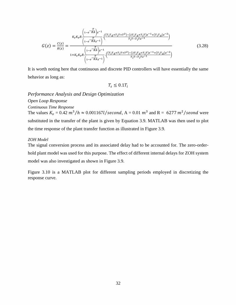
32
𝐺(𝑧) =𝐶(𝑧)
𝑅(𝑧)=
𝐾𝒄𝐾𝑣𝑅.
(1−𝑒−
𝑇𝑅𝐴)𝑧−1
(1−𝑒−
𝑇𝑅𝐴𝑧−1)
.((𝑇𝑖𝑇𝑑+𝑇𝑖𝑇+𝑇2)−(2𝑇𝑖𝑇𝑑+𝑇𝑖𝑇)𝑧−1+(𝑇𝑖𝑇𝑑)𝑧−2
𝑇𝑖𝑇−𝑇𝑖𝑇𝑧−1 )
1+𝐾𝒄𝐾𝑣𝑅.
(1−𝑒−
𝑇𝑅𝐴)𝑧−1
(1−𝑒−
𝑇𝑅𝐴𝑧−1)
.((𝑇𝑖𝑇𝑑+𝑇𝑖𝑇+𝑇2)−(2𝑇𝑖𝑇𝑑+𝑇𝑖𝑇)𝑧−1+(𝑇𝑖𝑇𝑑)𝑧−2
𝑇𝑖𝑇−𝑇𝑖𝑇𝑧−1 )
(3.28)
It is worth noting here that continuous and discrete PID controllers will have essentially the same
behavior as long as:
𝑇𝑠 ≤ 0.1𝑇𝑖
Performance Analysis and Design Optimization
Open Loop Response
Continuous Time Response
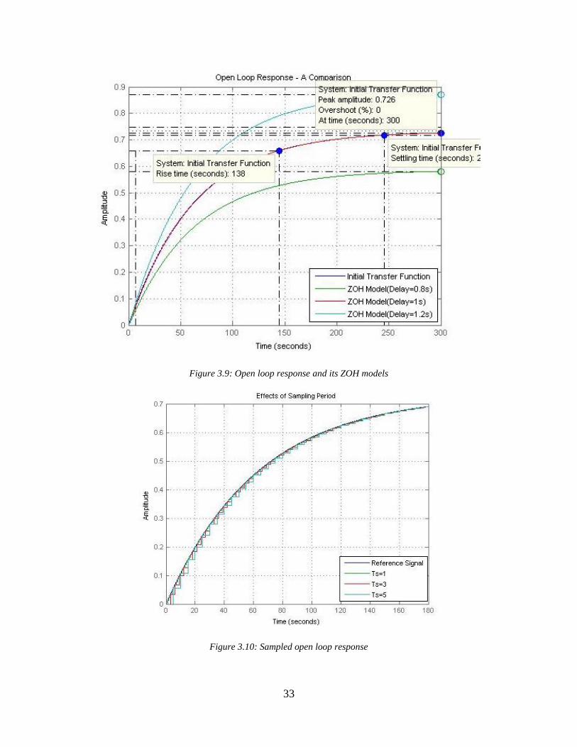
The values 𝐾𝑣 = 0.42 𝑚3 ℎ⁄ ≈ 0.001167𝑙 𝑠𝑒𝑐𝑜𝑛𝑑⁄ , A = 0.01 𝑚3 and R = 6277 𝑚2 𝑠𝑒𝑜𝑛𝑑⁄ were
substituted in the transfer of the plant is given by Equation 3.9. MATLAB was then used to plot
the time response of the plant transfer function as illustrated in Figure 3.9.
ZOH Model
The signal conversion process and its associated delay had to be accounted for. The zero-order-
hold plant model was used for this purpose. The effect of different internal delays for ZOH system
model was also investigated as shown in Figure 3.9.
Figure 3.10 is a MATLAB plot for different sampling periods employed in discretizing the
response curve.
33
Figure 3.9: Open loop response and its ZOH models
Figure 3.10: Sampled open loop response
34
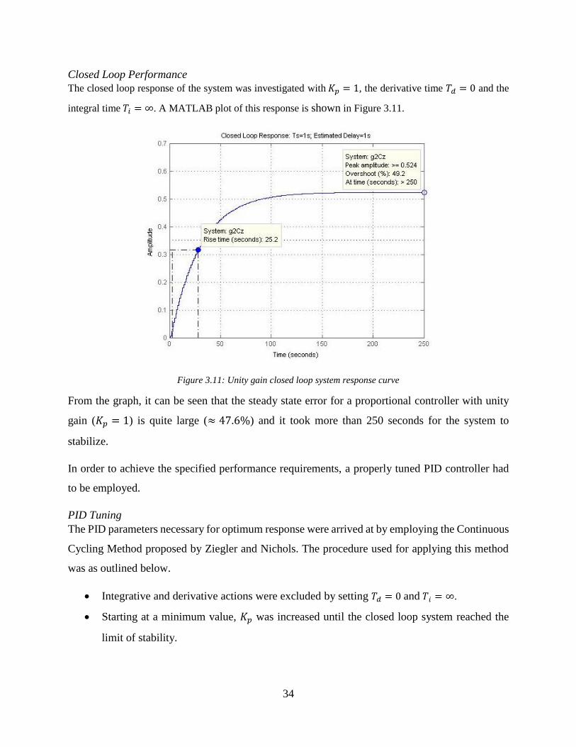
Closed Loop Performance
The closed loop response of the system was investigated with 𝐾𝑝 = 1, the derivative time 𝑇𝑑 = 0 and the
integral time 𝑇𝑖 = ∞. A MATLAB plot of this response is shown in Figure 3.11.
Figure 3.11: Unity gain closed loop system response curve
From the graph, it can be seen that the steady state error for a proportional controller with unity
gain (𝐾𝑝 = 1) is quite large (≈ 47.6%) and it took more than 250 seconds for the system to
stabilize.
In order to achieve the specified performance requirements, a properly tuned PID controller had
to be employed.
PID Tuning
The PID parameters necessary for optimum response were arrived at by employing the Continuous
Cycling Method proposed by Ziegler and Nichols. The procedure used for applying this method
was as outlined below.
Integrative and derivative actions were excluded by setting 𝑇𝑑 = 0 and 𝑇𝑖 = ∞.
Starting at a minimum value, 𝐾𝑝 was increased until the closed loop system reached the
limit of stability.
35
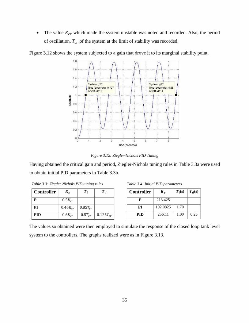
The value 𝐾𝑐𝑟 which made the system unstable was noted and recorded. Also, the period
of oscillation, 𝑇𝑐𝑟 of the system at the limit of stability was recorded.
Figure 3.12 shows the system subjected to a gain that drove it to its marginal stability point.
Figure 3.12: Ziegler-Nichols PID Tuning
Having obtained the critical gain and period, Ziegler-Nichols tuning rules in Table 3.3a were used
to obtain initial PID parameters in Table 3.3b.
Table 3.3: Ziegler Nichols PID tuning rules
Controller 𝑲𝒑 𝑻𝒊 𝑻𝒅
P 0.5𝐾𝑐𝑟
PI 0.45𝐾𝑐𝑟 0.85𝑇𝑐𝑟
PID 0.6𝐾𝑐𝑟 0.5𝑇𝑐𝑟 0.125𝑇𝑐𝑟
Table 3.4: Initial PID parameters
Controller 𝑲𝒑 𝑻𝒊(s) 𝑻𝒅(s)
P 213.425
PI 192.0825 1.70
PID 256.11 1.00 0.25
The values so obtained were then employed to simulate the response of the closed loop tank level
system to the controllers. The graphs realized were as in Figure 3.13.
36
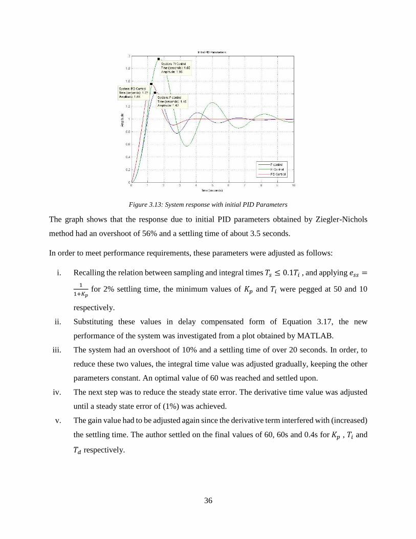
Figure 3.13: System response with initial PID Parameters
The graph shows that the response due to initial PID parameters obtained by Ziegler-Nichols
method had an overshoot of 56% and a settling time of about 3.5 seconds.
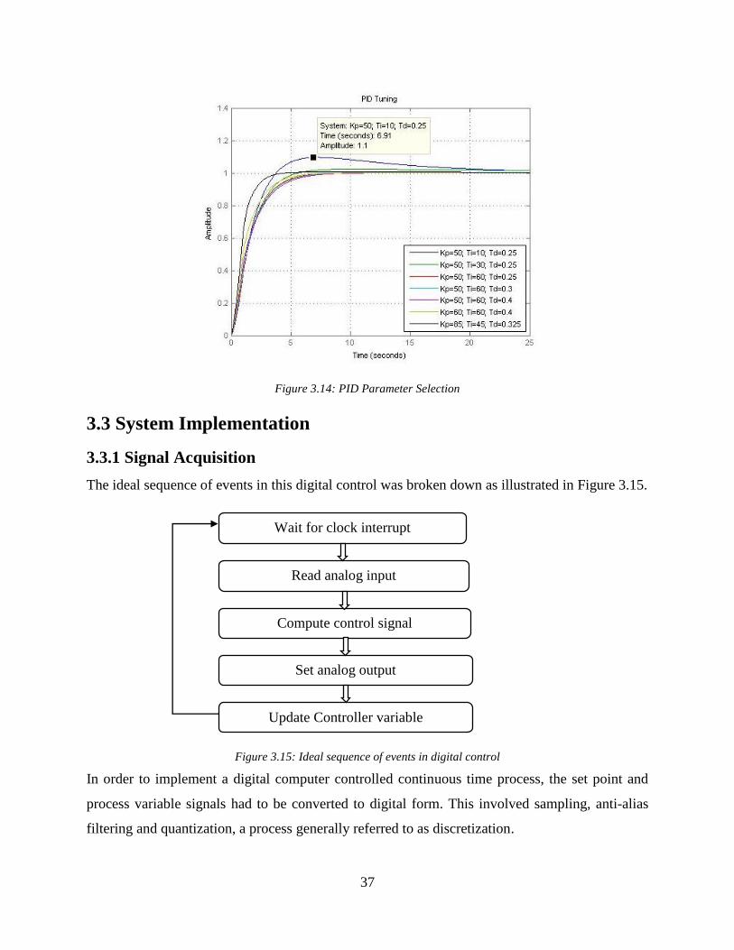
In order to meet performance requirements, these parameters were adjusted as follows:
i. Recalling the relation between sampling and integral times 𝑇𝑠 ≤ 0.1𝑇𝑖 , and applying 𝑒𝑠𝑠 =
1
1+𝐾𝑝 for 2% settling time, the minimum values of 𝐾𝑝 and 𝑇𝑖 were pegged at 50 and 10
respectively.
ii. Substituting these values in delay compensated form of Equation 3.17, the new
performance of the system was investigated from a plot obtained by MATLAB.
iii. The system had an overshoot of 10% and a settling time of over 20 seconds. In order, to
reduce these two values, the integral time value was adjusted gradually, keeping the other
parameters constant. An optimal value of 60 was reached and settled upon.
iv. The next step was to reduce the steady state error. The derivative time value was adjusted
until a steady state error of (1%) was achieved.
v. The gain value had to be adjusted again since the derivative term interfered with (increased)
the settling time. The author settled on the final values of 60, 60s and 0.4s for 𝐾𝑝 , 𝑇𝑖 and
𝑇𝑑 respectively.
37
Figure 3.14: PID Parameter Selection
3.3 System Implementation
3.3.1 Signal Acquisition
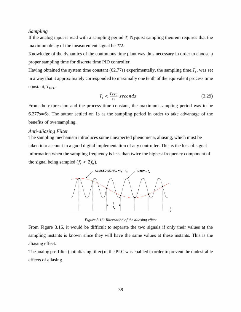
The ideal sequence of events in this digital control was broken down as illustrated in Figure 3.15.
Figure 3.15: Ideal sequence of events in digital control
In order to implement a digital computer controlled continuous time process, the set point and
process variable signals had to be converted to digital form. This involved sampling, anti-alias
filtering and quantization, a process generally referred to as discretization.
Wait for clock interrupt
Read analog input
Compute control signal
Set analog output
Update Controller variable
38
Sampling
If the analog input is read with a sampling period T, Nyquist sampling theorem requires that the
maximum delay of the measurement signal be T/2.
Knowledge of the dynamics of the continuous time plant was thus necessary in order to choose a
proper sampling time for discrete time PID controller.
Having obtained the system time constant (62.77s) experimentally, the sampling time,𝑇𝑠, was set
in a way that it approximately corresponded to maximally one tenth of the equivalent process time
constant, 𝑇𝐸𝑇𝐶 .
𝑇𝑠 <𝑇𝐸𝑇𝐶
10 𝑠𝑒𝑐𝑜𝑛𝑑𝑠 (3.29)
From the expression and the process time constant, the maximum sampling period was to be
6.277s≈6s. The author settled on 1s as the sampling period in order to take advantage of the
benefits of oversampling.
Anti-aliasing Filter
The sampling mechanism introduces some unexpected phenomena, aliasing, which must be
taken into account in a good digital implementation of any controller. This is the loss of signal
information when the sampling frequency is less than twice the highest frequency component of
the signal being sampled (𝑓𝑠 < 2𝑓𝑎).
Figure 3.16: Illustration of the aliasing effect
From Figure 3.16, it would be difficult to separate the two signals if only their values at the
sampling instants is known since they will have the same values at these instants. This is the
aliasing effect.
The analog pre-filter (antialiasing filter) of the PLC was enabled in order to prevent the undesirable
effects of aliasing.

39
Calibration
I/O Terminals Calibration
The analog inputs and output terminals of the PLC had to be calibrated according to the range of
input and output signals. The following steps were followed when calibrating the input
i. The power to the module was turned off and the desired input range was selected
using the configuration switches.
ii. After selecting the 0-10V range, the power to the CPU and module was turned on
and the module was allowed to stabilize for 15 minutes.
iii. Using a voltage source, a zero value voltage was applied to one of the input
terminals (AIW2). Using a ladder diagram program, the value reported to the CPU
by the input channel was read as the OFFSET calibration potentiometer was being
adjusted until the reading was the minimum possible.
iv. The same voltage source was then used to connect a full-scale value signal (10Vdc)
to the same input terminal and the value reported to the CPU was read while GAIN
calibration potentiometer was being adjusted until the reading was a desired
maximum (32000 bits).
Level Transducer Calibration
For proper signal conversion and manipulation, calibration of the sensors and actuators was
necessary.
In order to determine the transfer function of the level transducer, the following procedure was
followed.
With all discharge valves closed, the tank was filled to different levels of water and the
corresponding voltage from the signal conditioner was measured using a digital
multimeter. The values obtained were tabulated as in Table 3.1.
Digital equivalents of the sensor output, connected to analog input AIW4, were obtained
by examining the input terminal from the PLC using digital switch I1.1.
Proportional Valve Calibration
For this investigation, the following steps were undertaken by the author.
i. The solenoid valve was energized by applying 24Vdc from the PLC. The manual outlet
valve (V2) remained in closed position.

40
ii. The pump was switched ON and the control signal for the proportional valve was varied
while observing the rate of inflow as well as the rise in level of water in the tank. The
manual valve was opened accordingly with increasing rate of inflow in order to avoid
overflow of water. It was noted that with the control signal at its maximum, the rate of
inflow was 6.89 l/min, a value greater than the value required for this process (5 l/min).
iii. With the control signal held at its maximum, the manual valve (V1) in series with the
proportional valve was adjusted until a rate of inflow of 5.01 l/min was achieved.
iv. Starting from the minimum value, the control signal was varied in steps and corresponding
flow sensor voltages and flow rates were recorded as depicted in Table 3.2.
A voltage from the analog input (AIW2) was transferred to the analog output (AQW0) from where
it was fed to input of the power amplifier to provide the proportional valve control signal. The
potentiometer attached to the input AIW2 was adjusted to obtain the required steps of power
amplifier input. This procedure was enabled by digital switches I1.2 and I1.3.
3.3.2 Control Program Development
Introduction
The procedure for writing and testing software was divided into several stages, that is,
Input calibration.
ON/OFF control of water tank level.
PID control of water tank level
Modification of program to incorporate additional features deemed necessary to improve
the performance of the program and system in general.
Besides affirming the correctness of code, tests in the first two stages served to prove the
A-D/D-A conversion as well as the calibration of the PLC analog I/O terminals, the transducer and
the actuator.
Choice of Language
Ladder diagram programming was preferred to the other languages due to its simplicity and ease
of program debugging. The amount of sampling time achievable was not a criterion for settling on
the programming language since this was a slow process and the three languages were suitable in
as far as sampling period was concerned.
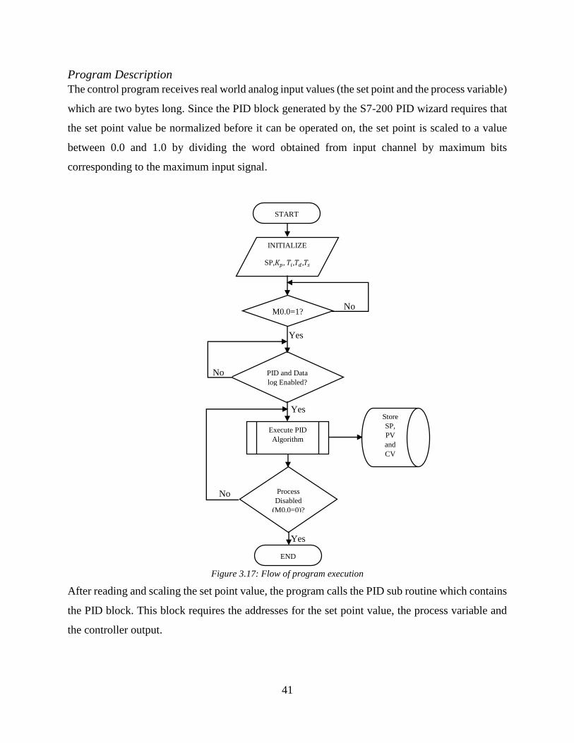
41
Program Description
The control program receives real world analog input values (the set point and the process variable)
which are two bytes long. Since the PID block generated by the S7-200 PID wizard requires that
the set point value be normalized before it can be operated on, the set point is scaled to a value
between 0.0 and 1.0 by dividing the word obtained from input channel by maximum bits
corresponding to the maximum input signal.
Figure 3.17: Flow of program execution
After reading and scaling the set point value, the program calls the PID sub routine which contains
the PID block. This block requires the addresses for the set point value, the process variable and
the controller output.
Yes
Yes
Yes
Yes
No
INITIALIZE
SP,𝐾𝑝, 𝑇𝑖,𝑇𝑑,𝑇𝑠
START
Execute PID
Algorithm
PID and Data
log Enabled?
Store
SP,
PV
and
CV
Process
Disabled
(M0.0=0)?
END
M0.0=1?
No
No
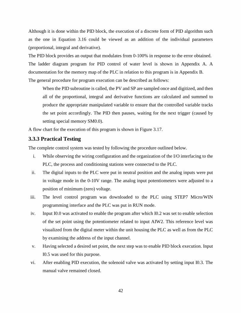
42
Although it is done within the PID block, the execution of a discrete form of PID algorithm such
as the one in Equation 3.16 could be viewed as an addition of the individual parameters
(proportional, integral and derivative).
The PID block provides an output that modulates from 0-100% in response to the error obtained.
The ladder diagram program for PID control of water level is shown in Appendix A. A
documentation for the memory map of the PLC in relation to this program is in Appendix B.
The general procedure for program execution can be described as follows:
When the PID subroutine is called, the PV and SP are sampled once and digitized, and then
all of the proportional, integral and derivative functions are calculated and summed to
produce the appropriate manipulated variable to ensure that the controlled variable tracks
the set point accordingly. The PID then pauses, waiting for the next trigger (caused by
setting special memory SM0.0).
A flow chart for the execution of this program is shown in Figure 3.17.
3.3.3 Practical Testing
The complete control system was tested by following the procedure outlined below.
i. While observing the wiring configuration and the organization of the I/O interfacing to the
PLC, the process and conditioning stations were connected to the PLC.
ii. The digital inputs to the PLC were put in neutral position and the analog inputs were put
in voltage mode in the 0-10V range. The analog input potentiometers were adjusted to a
position of minimum (zero) voltage.
iii. The level control program was downloaded to the PLC using STEP7 Micro/WIN
programming interface and the PLC was put in RUN mode.
iv. Input I0.0 was activated to enable the program after which I0.2 was set to enable selection
of the set point using the potentiometer related to input AIW2. This reference level was
visualized from the digital meter within the unit housing the PLC as well as from the PLC
by examining the address of the input channel.
v. Having selected a desired set point, the next step was to enable PID block execution. Input
I0.5 was used for this purpose.
vi. After enabling PID execution, the solenoid valve was activated by setting input I0.3. The
manual valve remained closed.
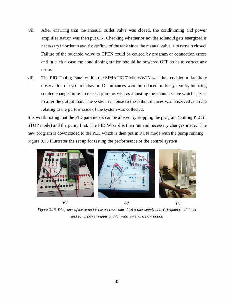
43
vii. After ensuring that the manual outlet valve was closed, the conditioning and power
amplifier station was then put ON. Checking whether or not the solenoid gets energized is
necessary in order to avoid overflow of the tank since the manual valve is to remain closed.
Failure of the solenoid valve to OPEN could be caused by program or connection errors
and in such a case the conditioning station should be powered OFF so as to correct any
errors.
viii. The PID Tuning Panel within the SIMATIC 7 Micro/WIN was then enabled to facilitate
observation of system behavior. Disturbances were introduced to the system by inducing
sudden changes in reference set point as well as adjusting the manual valve which served
to alter the output load. The system response to these disturbances was observed and data
relating to the performance of the system was collected.
It is worth noting that the PID parameters can be altered by stopping the program (putting PLC in
STOP mode) and the pump first. The PID Wizard is then run and necessary changes made. The
new program is downloaded to the PLC which is then put in RUN mode with the pump running.
Figure 3.18 illustrates the set up for testing the performance of the control system.
(a)
(b)
(c)
Figure 3.18: Diagrams of the setup for the process control (a) power supply unit, (b) signal conditioner
and pump power supply and (c) water level and flow station
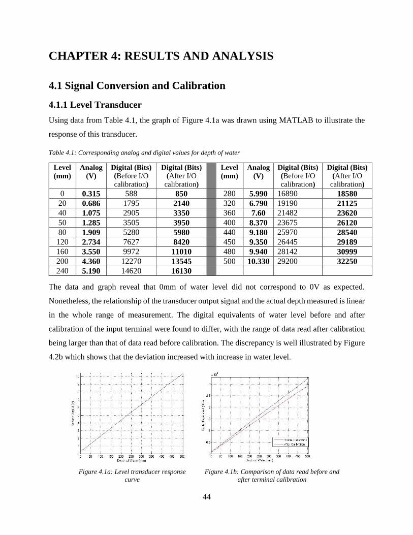
44
CHAPTER 4: RESULTS AND ANALYSIS
4.1 Signal Conversion and Calibration
4.1.1 Level Transducer
Using data from Table 4.1, the graph of Figure 4.1a was drawn using MATLAB to illustrate the
response of this transducer.
Table 4.1: Corresponding analog and digital values for depth of water
Level
(mm)
Analog
(V) Digital (Bits)
(Before I/O
calibration)
Digital (Bits)
(After I/O
calibration)
Level
(mm)
Analog
(V) Digital (Bits)
(Before I/O
calibration)
Digital (Bits)
(After I/O
calibration)
0 0.315 588 850 280 5.990 16890 18580
20 0.686 1795 2140 320 6.790 19190 21125
40 1.075 2905 3350 360 7.60 21482 23620
50 1.285 3505 3950 400 8.370 23675 26120
80 1.909 5280 5980 440 9.180 25970 28540
120 2.734 7627 8420 450 9.350 26445 29189
160 3.550 9972 11010 480 9.940 28142 30999
200 4.360 12270 13545 500 10.330 29200 32250
240 5.190 14620 16130
The data and graph reveal that 0mm of water level did not correspond to 0V as expected.
Nonetheless, the relationship of the transducer output signal and the actual depth measured is linear
in the whole range of measurement. The digital equivalents of water level before and after
calibration of the input terminal were found to differ, with the range of data read after calibration
being larger than that of data read before calibration. The discrepancy is well illustrated by Figure
4.2b which shows that the deviation increased with increase in water level.
Figure 4.1a: Level transducer response
curve
Figure 4.1b: Comparison of data read before and
after terminal calibration

45
4.1.2 Proportional Valve
Table 4.2 illustrates data collected from the proportional valve calibration procedure.
The table shows corresponding values for the rate of flow (l/min) of water into the tank, the flow
sensor output (V) and the valve control signal (V) that were recorded for each input voltage to the
power amplifier.
The table also shows the voltage at the output AQW0 and that at the input to the power amplifier.
Table 4.2: Analog control signal and corresponding flow rate
Output
voltage (At AQW0)
Input
voltage (At Power amplifier)
Valve
Control
Signal
(V)
Flow
Rate
(l/min)
Sensor
Output
(V)
Output
voltage
(At AQW0)
Input
voltage (At Power amplifier)
Valve
Control
Signal
(V)
Flow
Rate
(l/min)
Sensor
Output
(V)
0.01 0.0346 2.587 2.61 5.4 6.0 5.96 13.23 4.64 9.58
0.5 0.453 3.453 2.73 5.64 6.5 6.47 14.10 4.70 9.70
1.0 0.96 4.34 2.87 5.94 6.75 6.73 14.52 4.78 9.85
1.5 1.457 5.22 3.08 6.41 7.0 6.97 15.01 4.83 9.96
2.0 1.959 6.10 3.26 6.75 7.5 7.47 15.83 4.92 9.98
2.5 2.466 7.00 3.49 7.22 8.0 7.96 16.78 4.92 10.01
3.0 2.968 7.89 3.67 7.58 8.5 8.47 17.65 4.93 10.14
3.5 3.464 8.78 3.93 7.91 9.0 8.97 18.50 4.98 10.31
4.0 3.97 9.68 4.01 8.32 9.5 9.47 19.15 5.00 10.33
4.5 4.47 10.57 4.20 8.64 10.0 9.97 19.67 5.01 10.34
5.0 4.96 11.44 4.35 8.96 10.25 10.22 19.90 5.01 10.34
5.5 5.46 12.33 4.50 9.25
Figure 4.2: Relation between flowrate, sensor
output and valve control signals
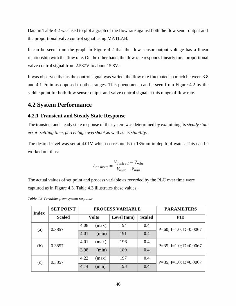
46
Data in Table 4.2 was used to plot a graph of the flow rate against both the flow senor output and
the proportional valve control signal using MATLAB.
It can be seen from the graph in Figure 4.2 that the flow sensor output voltage has a linear
relationship with the flow rate. On the other hand, the flow rate responds linearly for a proportional
valve control signal from 2.587V to about 15.8V.
It was observed that as the control signal was varied, the flow rate fluctuated so much between 3.8
and 4.1 l/min as opposed to other ranges. This phenomena can be seen from Figure 4.2 by the
saddle point for both flow sensor output and valve control signal at this range of flow rate.
4.2 System Performance
4.2.1 Transient and Steady State Response
The transient and steady state response of the system was determined by examining its steady state
error, settling time, percentage overshoot as well as its stability.
The desired level was set at 4.01V which corresponds to 185mm in depth of water. This can be
worked out thus:
𝐿𝑑𝑒𝑠𝑖𝑟𝑒𝑑 =𝑉𝑑𝑒𝑠𝑖𝑟𝑒𝑑 − 𝑉𝑚𝑖𝑛
𝑉𝑚𝑎𝑥 − 𝑉𝑚𝑖𝑛
The actual values of set point and process variable as recorded by the PLC over time were
captured as in Figure 4.3. Table 4.3 illustrates these values.
Table 4.3 Variables from system response
Index SET POINT PROCESS VARIABLE PARAMETERS
Scaled Volts Level (mm) Scaled PID
(a) 0.3857 4.08 (max) 194 0.4
P=60; I=1.0; D=0.0067 4.01 (min) 191 0.4
(b) 0.3857 4.01 (max) 196 0.4
P=35; I=1.0; D=0.0067 3.98 (min) 189 0.4
(c) 0.3857 4.22 (max) 197 0.4
P=85; I=1.0; D=0.0067 4.14 (min) 193 0.4

47
(a)
(b)
(c)
Figure 4.3: System performance for (a) t=0, (b) transient response and
(c) steady state response
The various signals in Figure 4.3 are color coded such that:
Red – Process variable
Green – Set point
Blue – Manipulated variable
It was noted that the scaled value for the process value was rounded off to the nearest one decimal
by the PLC. Also, the scaled value of the set point was not 0.401 as expected revealing a
discretization error of:
(0.4010 − 0.3857)
0.4010∗ 100 = 3.8155%
The desired level of water from the scaled value of the set point can be given by:
0.3857
1.0000∗ 500 = 192.85 ≅ 193𝑚𝑚

48
It can be seen from Table 4.3 and Figure 4.3 that the system had the following performance
characteristics:
Steady state error = |192.85−191|
192.85∗ 100 = 0.9593%
Settling time ≅ 55 − 13 = 42𝑠
Percentage overshoot = 0%
Stability - System stable
A z-plane analysis showed that the system was stable since all poles were within the unit circle.
This is shown in Figure 4.4. The poles and zeros from Figure 4.4 are as in Table 4.4.
Figure 4.4: z plane analysis of system
performance
Table 4.4: System poles and zeros
Poles -0.5247
0.9835
0.5395
Zeros 0.9835
0.2871
4.2.2 Effects of Parameter Variation
Process Delay
Figure 3.9 reveals that an internal delay approximation of 1 second in ZOH modelling of the plant
transfer function tracked the initial plant transfer function quite satisfactorily. However, delay
approximations of 0.8 and 1.2 seconds resulted in under and over estimation of the plant transfer
function respectively.
Process Gain
When all other parameters were held constant and the process gain was varied, the results were as
in Figure 4.5.

49
(i)
(ii)
Figure 4.5a: (i) transient and (ii) steady state responses with gain=35
(i)
(ii)
Figure 4.5b: (i) transient and (ii) steady state responses with gain=85
It can be seen from Figure 3.5 that the system settling time was 45s with 𝐾𝑝 = 85 and 40s
with 𝐾𝑝 = 85. The settling time is thus shorter with a higher gain and longer with a lower gain.
The steady state errors for the system when the different gains were applied was higher than that
with proportional gain of 60. That is,
|192.85−189|
192.85∗ 100 = 1.9964% (for 𝐾𝑝 = 35)
|192.85−197|
192.85∗ 100 = 2.1519% (for 𝐾𝑝 = 85)
Sampling Time
Figure 4.6 illustrates the system response when all other parameters except the sampling time were
held constant.
With sampling periods of 0.1s and 5s, the process variable first increased at a high rate before
slowing down until it could track the set point. For 10s sampling period, the increase of the process
variable was smooth from the beginning to the point at which it could track the set point.
An examination of the steady state response revealed that the process variable could not track the
set point to the required accuracy level with these sampling periods. The accuracy was better with
𝑇𝑠 = 0.1𝑠 as opposed to when it was 5s or 10s.
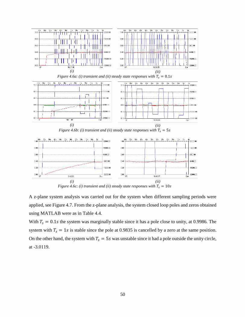
50
(i)
(ii)
Figure 4.6a: (i) transient and (ii) steady state responses with 𝑇𝑠 = 0.1𝑠
(i)
(ii)
Figure 4.6b: (i) transient and (ii) steady state responses with 𝑇𝑠 = 5𝑠
(i)
(ii)
Figure 4.6c: (i) transient and (ii) steady state responses with 𝑇𝑠 = 10𝑠
A z-plane system analysis was carried out for the system when different sampling periods were
applied, see Figure 4.7. From the z-plane analysis, the system closed loop poles and zeros obtained
using MATLAB were as in Table 4.4.
With 𝑇𝑠 = 0.1𝑠 the system was marginally stable since it has a pole close to unity, at 0.9986. The
system with 𝑇𝑠 = 1𝑠 is stable since the pole at 0.9835 is cancelled by a zero at the same position.
On the other hand, the system with 𝑇𝑠 = 5𝑠 was unstable since it had a pole outside the unity circle,
at -3.0119.

51
(𝑇𝑠 = 0.1𝑠) (𝑇𝑠 = 1𝑠) (𝑇𝑠 = 5𝑠)
Figure 4.7: Effect of sampling period on system stability
Table 4.5: Closed loop poles and zeros for various 𝑇𝑠
Sampling Period 0.1s 1s 5s
Poles 0.9986
0.9449
-0.3052
0.9835
0.5395
-0.5247
0.9226
0.096
-3.0119
Zeros 0.9983
0.8011
0.9835
0.2871
0.9226
0.0745
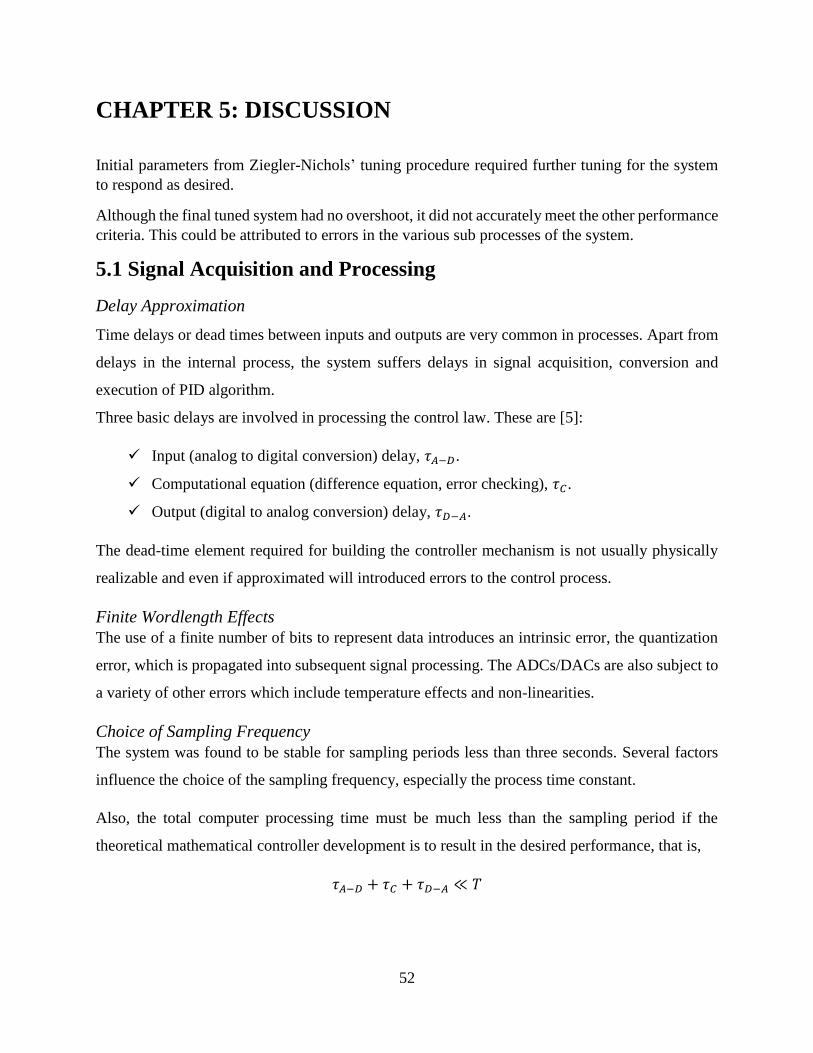
52
CHAPTER 5: DISCUSSION
Initial parameters from Ziegler-Nichols’ tuning procedure required further tuning for the system
to respond as desired.
Although the final tuned system had no overshoot, it did not accurately meet the other performance
criteria. This could be attributed to errors in the various sub processes of the system.
5.1 Signal Acquisition and Processing
Delay Approximation
Time delays or dead times between inputs and outputs are very common in processes. Apart from
delays in the internal process, the system suffers delays in signal acquisition, conversion and
execution of PID algorithm.
Three basic delays are involved in processing the control law. These are [5]:
Input (analog to digital conversion) delay, 𝜏𝐴−𝐷.
Computational equation (difference equation, error checking), 𝜏𝐶.
Output (digital to analog conversion) delay, 𝜏𝐷−𝐴.
The dead-time element required for building the controller mechanism is not usually physically
realizable and even if approximated will introduced errors to the control process.
Finite Wordlength Effects
The use of a finite number of bits to represent data introduces an intrinsic error, the quantization
error, which is propagated into subsequent signal processing. The ADCs/DACs are also subject to
a variety of other errors which include temperature effects and non-linearities.
Choice of Sampling Frequency
The system was found to be stable for sampling periods less than three seconds. Several factors
influence the choice of the sampling frequency, especially the process time constant.
Also, the total computer processing time must be much less than the sampling period if the
theoretical mathematical controller development is to result in the desired performance, that is,
𝜏𝐴−𝐷 + 𝜏𝐶 + 𝜏𝐷−𝐴 ≪ 𝑇
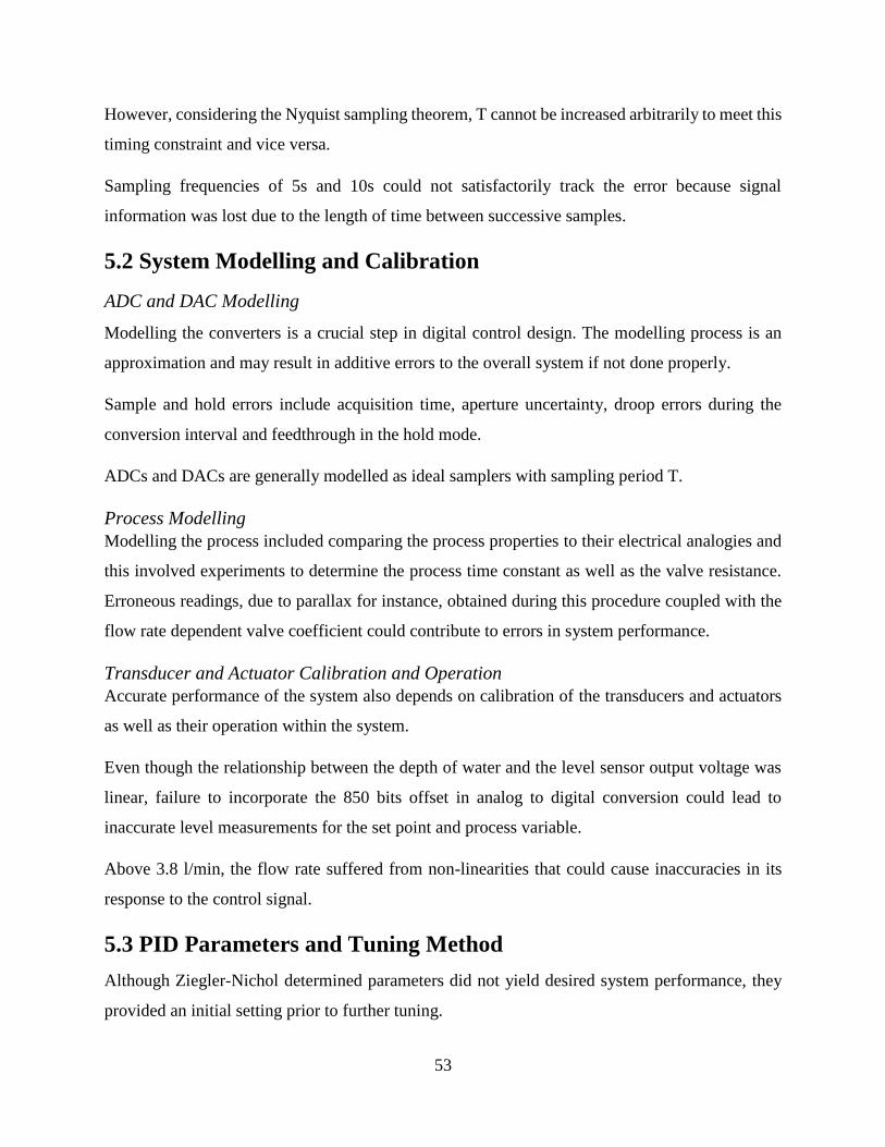
53
However, considering the Nyquist sampling theorem, T cannot be increased arbitrarily to meet this
timing constraint and vice versa.
Sampling frequencies of 5s and 10s could not satisfactorily track the error because signal
information was lost due to the length of time between successive samples.
5.2 System Modelling and Calibration
ADC and DAC Modelling
Modelling the converters is a crucial step in digital control design. The modelling process is an
approximation and may result in additive errors to the overall system if not done properly.
Sample and hold errors include acquisition time, aperture uncertainty, droop errors during the
conversion interval and feedthrough in the hold mode.
ADCs and DACs are generally modelled as ideal samplers with sampling period T.
Process Modelling
Modelling the process included comparing the process properties to their electrical analogies and
this involved experiments to determine the process time constant as well as the valve resistance.
Erroneous readings, due to parallax for instance, obtained during this procedure coupled with the
flow rate dependent valve coefficient could contribute to errors in system performance.
Transducer and Actuator Calibration and Operation
Accurate performance of the system also depends on calibration of the transducers and actuators
as well as their operation within the system.
Even though the relationship between the depth of water and the level sensor output voltage was
linear, failure to incorporate the 850 bits offset in analog to digital conversion could lead to
inaccurate level measurements for the set point and process variable.
Above 3.8 l/min, the flow rate suffered from non-linearities that could cause inaccuracies in its
response to the control signal.
5.3 PID Parameters and Tuning Method
Although Ziegler-Nichol determined parameters did not yield desired system performance, they
provided an initial setting prior to further tuning.

54
Varying the process gain with the other parameters held constant affected the system response time
and no effect on the overshoot up to a gain value of 85. On the other hand, a change in sampling
period with other parameters held constant had a profound effect on system stability as illustrated
by Figure 4.7.
In PID control, high proportional gain results in a large change in the output for a given change in
the error. If the proportional gain is too high, the system can become unstable. In contrast, a small
gain results in a small output response to a large input error, and a less responsive controller. Other
practical issues in the application of PID control include:
Processes have physical constraints, for instance, pumps have limited power. These
limitations can be regarded as non-linearities in the process and have to be considered in
the application of the controller. These limitations and are usually modeled with a non-
linear element having a saturation characteristic, as shown in Figure 5.1.
Figure 5.1: Input limitation as part of the control system
Beside input magnitude limitations, actuators often have defined rate limitations, or
maximum rates at which the control signal 𝑢(𝑡) can be changed. When the controller output
signal 𝑢0(𝑡) exceeds the upper limit 𝑢𝑚𝑎𝑥 or when it falls below the lower limit 𝑢𝑚𝑖𝑛 of
the operating range, its value changes in the input limitation element so that the controller
output signal 𝑢0(𝑡) and the process input 𝑢(𝑡) do not coincide. Shouldn’t the two coincide,
the integrator in a controller with integral action would produce an inaccurate and highly
excessive value which would cause oscillation and slowing down of the transient response.
In other words, the effect would be a large overshoot and a long settling time.
5.4 Assumptions
Some process dynamics are difficult to model mathematically and therefore may end up not being
accounted for in the design even though they can affect the accuracy of fluid measurement.

55
In modelling and designing this control system, several assumptions were made that could have
resulted in system performance inaccuraies.
Idealized Tank Level Process System
Level process is linear.
All inflow goes to outflow, the tank is merely a buffer storage tank.
Level ontroller set point is constant, that is, it is rarely changed.
Up or downstream pressure, line loss or pump curve have no effect on loop behaviour.
Changes in pressure are small and the fluid in question (water) is incompressible and has a
constant density.
The value of Kv in Equation 3.9 remained constant regardless of changes in the rate of
flow or the area of restriction.
The speed of response of the flow loop (the time constant of the unit transducer signal
conditioner) is significantly faster than that of the level in the tank (control process);
therefore, the dynamic can be ignored.
ZOH Model of the ADC and DAC
ADC outputs are exactly equal in magnitude to their inputs, that is, quantization errors are
negligible.
The ADC yields a digital output instantaneously.
Sampling is perfectly uniform, that is, occurs at a fixed rate.
DAC outputs are exactly equal in magnitude to their inputs.
The DAC yields an analog output instantaneously.
DAC outputs are constant over each sampling period
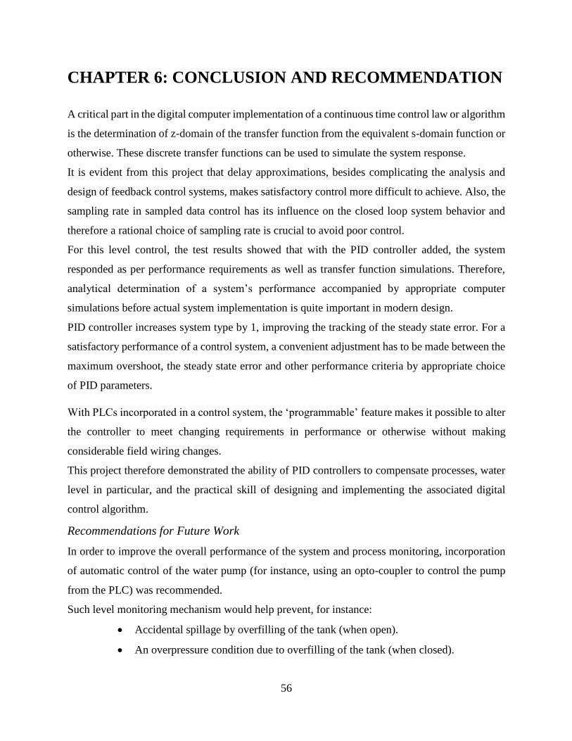
56
CHAPTER 6: CONCLUSION AND RECOMMENDATION
A critical part in the digital computer implementation of a continuous time control law or algorithm
is the determination of z-domain of the transfer function from the equivalent s-domain function or
otherwise. These discrete transfer functions can be used to simulate the system response.
It is evident from this project that delay approximations, besides complicating the analysis and
design of feedback control systems, makes satisfactory control more difficult to achieve. Also, the
sampling rate in sampled data control has its influence on the closed loop system behavior and
therefore a rational choice of sampling rate is crucial to avoid poor control.
For this level control, the test results showed that with the PID controller added, the system
responded as per performance requirements as well as transfer function simulations. Therefore,
analytical determination of a system’s performance accompanied by appropriate computer
simulations before actual system implementation is quite important in modern design.
PID controller increases system type by 1, improving the tracking of the steady state error. For a
satisfactory performance of a control system, a convenient adjustment has to be made between the
maximum overshoot, the steady state error and other performance criteria by appropriate choice
of PID parameters.
With PLCs incorporated in a control system, the ‘programmable’ feature makes it possible to alter
the controller to meet changing requirements in performance or otherwise without making
considerable field wiring changes.
This project therefore demonstrated the ability of PID controllers to compensate processes, water
level in particular, and the practical skill of designing and implementing the associated digital
control algorithm.
Recommendations for Future Work
In order to improve the overall performance of the system and process monitoring, incorporation
of automatic control of the water pump (for instance, using an opto-coupler to control the pump
from the PLC) was recommended.
Such level monitoring mechanism would help prevent, for instance:
Accidental spillage by overfilling of the tank (when open).
An overpressure condition due to overfilling of the tank (when closed).
57
References
[1] Farid Golnaraghi, Benjamin C. Kuo - Automatic Control Systems, John Wiley & Sons Inc.,
9TH Edition.
[2] Norman S. Nise - Control Systems Engineering, John Wiley & Sons, Inc., Sixth Edition
[3] Roland S. Burns - Advanced Control Engineering, Butterworth Heinemann.
[4] D. Ibrahim - Microcontroller Based Applied Digital Control, John Wiley & Sons Ltd.
[5] John J. D’Azzo and Constantine H. Houpis, Stuart N. Sheldon - Linear Control System
Analysis and Design with MATLAB, Marcel Dekker Inc., 5th edition.
[6] Katsuhiko Ogata - Modern Control Engineering, Prentice-Hall Inc., 4th Edition.
[7] L. A. Bryan and E. A. Bryan – Programmable Controllers: Theory and Implementation,
Industrial Text Company, 2nd Edition.
[8] W. Bolton – Programmable Logic Controllers, Elsevier Newnes, 4th Edition.
[9] Stephen Boyd and Craig Barratt - Linear Controller Design: Limits of Performance, Prentice-
Hall, 1991.
[10] Raymond A. Serway and John W. Jewett, Jr. - Physics for Scientists and Engineers with
Modern Physics, 8th Edition, Mary Finch, 2010
[11] Roy Ball and Roger Pratt – Engineering Applications of Microcomputers: Instrumentation
and Control, Prentice Hall International, Incorporated, 1986.
[12] Constantine H. Houpis and Gary B. Lamont - Digital Control Systems (Theory, Hardware,
Software), McGraw-Hill Inc., 1985.
[13] Thomas E. Marlin, Process Control: Designing Processes and Control Systems for Dynamic
Performance, 2nd Edition, McMaster University, 2015.
[14] Dr. N.C. Jagan, Control Systems, 2nd Edition, BS Publications, 2008.
[15] Richard C. Dorf and Robert H. Bishop, Modern Control Systems, 11th Edition, Pearson
Prentice Hall, 2008.
[16] Biswanath Paul, Industrial Electronics and Control: Including Programmable Logic
Controller, 2nd Edition, PHI Learning Private Ltd, New Delhi, 2009.
58
[17] Texas Instruments, C2000™ Digital Controller Library User’s Guide, Literature number
SPRUI31, July 2015.
[18] Cecil L. Smith, Practical Process Control: Tuning and Troubleshooting, John Wiley &
Sons, Inc., 2009.
[19] M. Sami Fadali and Antonio Visioli, Digital Control Engineering: Analysis and Design, 2nd
Ed., Academic Press, Oxford, 2013.
[20] Antonio Visioli, Practical PID Control: Advances in Industrial Control series, Springer
Verlog Limited, 2006.
[21] Emmanuel C. Ifeachor and Barrie W. Jervis, Digital Signal Processing: A Practical
Approach, 2nd Ed., Pearson Education Limited, 2002.
[22] J. C. Basilio and S. R. Matos, Design of PI and PID Controllers With Transient
Performance Specification, IEEE Transactions On Education, Vol. 45, No. 4, November 2002.
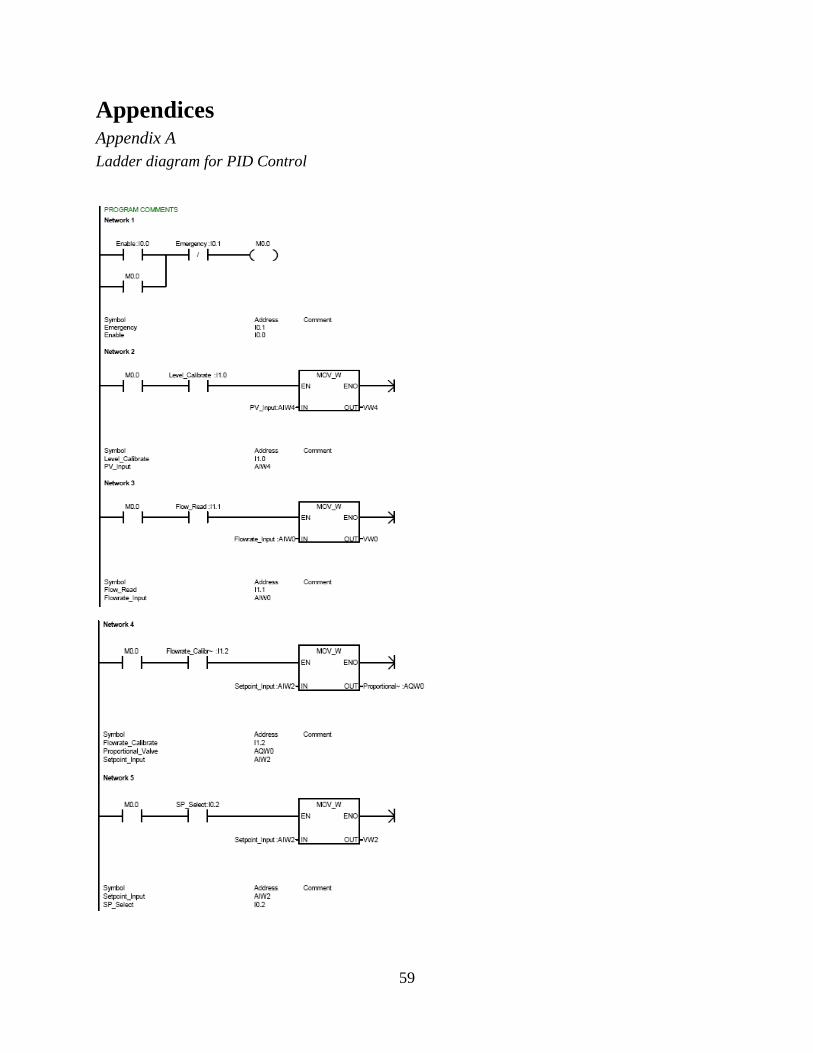
59
Appendices Appendix A
Ladder diagram for PID Control
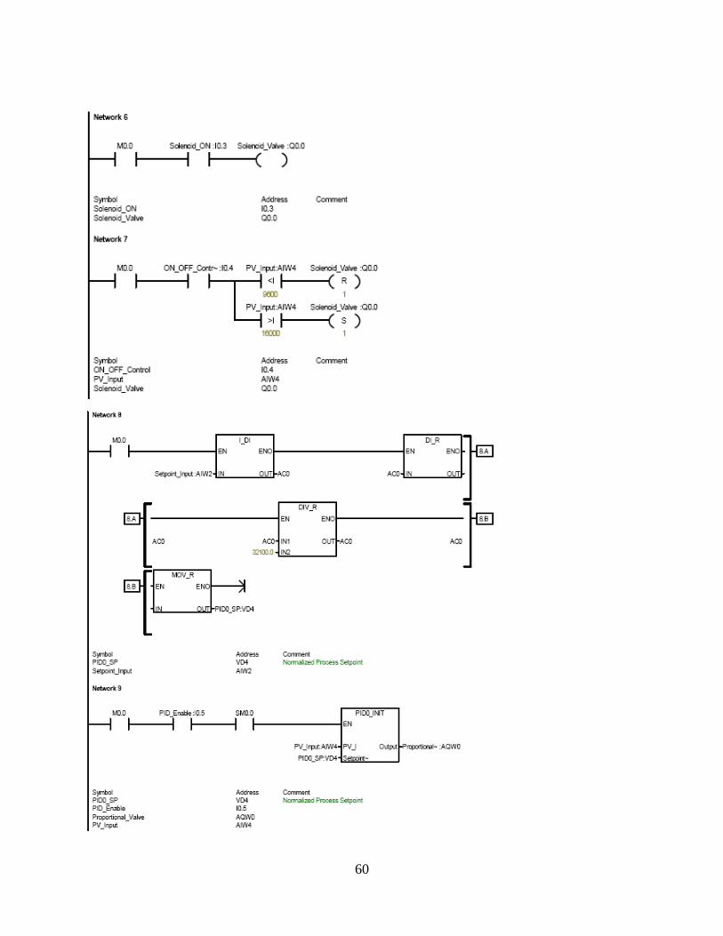
60

61
Appendix B
Software Documentation
TYPE OF SYMBOL ADDRESS DESCRIPTION
Inputs AIW0 Flow rate input
AIW2 Set point input
AIW4 Process variable input
I0.0 Program enable
I0.1 Program disable
I0.2 Enable selection of set point
I0.3 Activate solenoid valve
I0.4 Enable ON/OFF process control
I0.5 Enable PID execution and data logging blocks
I1.0 Enable reading of water level and sensor calibration
I1.1 Enable reading of rate of flow of water
I1.2 Enable flow sensor calibration
Outputs AQW0 Proportional valve control signal output
Q0.0 Solenoid valve activation/deactivation signal
PID Loop Table VB0 PID table address
VD0 Process variable (Scaled)
VD4 Set point (Scaled)
VD8 Output (Scaled)
VD12 Gain
VD16 Sample time
VD20 Integral time
VD24 Derivative time
VW80 Derivative counter
I/O Storage M0.0 Output storage area for indicating that the program has
been enabled
LW0 Process variable input (INT)
LD2 Set point input (REAL)
VW0 Flow rate
VW2 Set Point
VW4 Level (Process Variable)