Decision Trees for Functional Variables - DIMACS Trees for Functional Variables Suhrid Balakrishnan...
8
Decision Trees for Functional Variables Suhrid Balakrishnan Department of Computer Science Rutgers University Piscataway, NJ 08854, USA David Madigan Department of Statistics Rutgers University Piscataway, NJ 08854, USA Abstract Classification problems with functionally structured input variables arise naturally in many applications. In a clinical domain, for example, input variables could include a time series of blood pressure measurements. In a financial setting, different time series of stock returns might serve as predictors. In an archeological application, the 2-D pro- file of an artifact may serve as a key input variable. In such domains, accuracy of the classifier is not the only reasonable goal to strive for; classifiers that provide easily in- terpretable results are also of value. In this work, we present an intuitive scheme for ex- tending decision trees to handle functional input variables. Our results show that such decision trees are both accurate and readily interpretable. 1 INTRODUCTION We present an extension to standard decision trees (for example CART, Breiman et al. 1984 or C4.5, Quinlan 1993) that enables them to be applied to classification problems with functional data as inputs. In so doing, we aim to leverage the interpretability of decision trees as well as their other important benefits like reason- able classification performance and efficient associated learning procedures. The application that motivated this work concerns vaccine efficacy. The study in question followed thirty vaccinated non-human primates (NHPs) for a year and then “challenged” the animals. Of the 30 NHPs, 21 survived the challenge and 9 died. Repeated measure- ments during the year assessed over a dozen aspects of the putative immune response. These measure- ments include an immunoglobulin G enzyme-linked immunosorbent assay (IgG), various interleukin mea- sures (IL2, IL4, IL6), and a so-called “stimulation in- dex” (SI), to name a few, with the number of measure- ments varying somewhat from animal to animal. The goal of the study is to understand the predictive value of the various assays with respect to survival. 0 10 20 30 40 50 0 2 4 6 8 IgG, 9 dead (red), 21 survived (green) 0 10 20 30 40 50 0 1 2 3 4 IL6 Figure 1: IgG and IL6 measurements for all 30 NHPs. Green (solid) represents animals that survived; red (dashed) represents animals that died. The thick curves represent sample means. Our initial approach to this problem used a logistic regression model (Genkin et al., 2004) and treated each assay-timepoint combination as a separate input variable. While this provided good predictive perfor- mance, it selected a biologically meaningless set of predictors such as IgG at week 46, SI at week 38, and IL6 at week 12. The study immunologists in- stead sought insights such as “IgG trajectories that rise more rapidly after the 4-week booster shot and fall more slowly after the 26-week booster lead to higher survival probability.” In other words, the underlying
Transcript of Decision Trees for Functional Variables - DIMACS Trees for Functional Variables Suhrid Balakrishnan...

Decision Trees for Functional Variables
Suhrid BalakrishnanDepartment of Computer Science
Rutgers UniversityPiscataway, NJ 08854, USA
David MadiganDepartment of Statistics
Rutgers UniversityPiscataway, NJ 08854, USA
Abstract
Classification problems with functionallystructured input variables arise naturally inmany applications. In a clinical domain, forexample, input variables could include a timeseries of blood pressure measurements. Ina financial setting, different time series ofstock returns might serve as predictors. Inan archeological application, the 2-D pro-file of an artifact may serve as a key inputvariable. In such domains, accuracy of theclassifier is not the only reasonable goal tostrive for; classifiers that provide easily in-terpretable results are also of value. In thiswork, we present an intuitive scheme for ex-tending decision trees to handle functionalinput variables. Our results show that suchdecision trees are both accurate and readilyinterpretable.
1 INTRODUCTION
We present an extension to standard decision trees (forexample CART, Breiman et al. 1984 or C4.5, Quinlan1993) that enables them to be applied to classificationproblems with functional data as inputs. In so doing,we aim to leverage the interpretability of decision treesas well as their other important benefits like reason-able classification performance and efficient associatedlearning procedures.
The application that motivated this work concernsvaccine efficacy. The study in question followed thirtyvaccinated non-human primates (NHPs) for a year andthen “challenged” the animals. Of the 30 NHPs, 21survived the challenge and 9 died. Repeated measure-ments during the year assessed over a dozen aspectsof the putative immune response. These measure-ments include an immunoglobulin G enzyme-linked
immunosorbent assay (IgG), various interleukin mea-sures (IL2, IL4, IL6), and a so-called “stimulation in-dex” (SI), to name a few, with the number of measure-ments varying somewhat from animal to animal. Thegoal of the study is to understand the predictive valueof the various assays with respect to survival.
0 10 20 30 40 500
2
4
6
8IgG, 9 dead (red), 21 survived (green)
0 10 20 30 40 500
1
2
3
4IL6
Figure 1: IgG and IL6 measurements for all 30 NHPs.Green (solid) represents animals that survived; red(dashed) represents animals that died. The thickcurves represent sample means.
Our initial approach to this problem used a logisticregression model (Genkin et al., 2004) and treatedeach assay-timepoint combination as a separate inputvariable. While this provided good predictive perfor-mance, it selected a biologically meaningless set ofpredictors such as IgG at week 46, SI at week 38,and IL6 at week 12. The study immunologists in-stead sought insights such as “IgG trajectories thatrise more rapidly after the 4-week booster shot and fallmore slowly after the 26-week booster lead to highersurvival probability.” In other words, the underlying

biology suggests that the shape of the assay curvesshould be predictive of survival rather than measure-ments at specific timepoints. Figure 1, for example,shows IgG and IL6 trajectories. For IgG, comparisonof the thick green curve with the thick red curve showsthat higher values are beneficial at the beginning, thenlower values, and then higher values again towards theend. For IL6, it appears higher values of the curve ingeneral are beneficial. We shall return to the motivat-ing example in later sections.
More generally, we consider the following multi-classclassification problem: the training dataset comprisesn labeled training examples, D = {(xi, yi)}n
i=1 wherexi = [xi1, . . . ,xid] is a list of d features and yi ∈{1, . . . , c}, the c labels. We account for functionallystructured input data, by allowing the elements ofxi to be vectors/lists themselves, each representingan instance of a function of some independent vari-able. For example, a time series classification prob-lem with only one time-series (or functional) variableof fixed-length T say, as input, would be representedas xi = xi1 in our setup, with the single featurexi1 = [x(1)
i1 , x(2)i1 , . . . , x
(T )i1 ]. Here time would be the
independent variable.
We allow the inputs to be multivariate—meaningthere may be more than one functional variable(i.e., more than one vector/list element of xi)and also allow for standard (non-functional) dis-crete/continuous/categorical variables (in this case therelevant components of xi will be the correspondingscalars/nominal values). Thus, standard decision treescan be considered a type of special case of the aboveformulation where all inputs are restricted to length 1.
2 PREVIOUS STUDIES
Past approaches to this problem applying standardmachine learning algorithms have typically relied onsome sort of ad hoc and domain specific preprocessingto extract predictive features. A few previous studieslook for interesting “events” in the training instancesof the functional variables and then construct auxil-iary variables based on them. These auxiliary vari-ables are then used by either a particular classifier (de-cision trees, regression trees and 1-nearest neighbor,Geurts 2001 which retains interpretability), or genericclassifiers (Kadous and Sammut, 2005) (with inter-pretable results available if a rule learning classifier isapplied), or used in literals as base classifiers combinedvia boosting (Gonzalez and Diez, 2004). Another ap-proach is the scheme by Kudo et al. (1999), whichconstrains the functional variables to pass through cer-tain regions in (discretized) space and disallows otherregions. There are also techniques that create fea-
tures via specialized functional PCA techniques, de-signed to deal with large data applications (EEG data)where the functional variables are lengthy and numer-ous. Finally, there are support vector machine basedapproaches that are typically applied by defining anappropriate kernel function for the problem domain(Shimodaira et al., 2001).
3 CANDIDATE SPLITS FORFUNCTIONAL VARIABLES
In order for a decision tree to be able to process func-tional variables, we first need to define candidate splitsfor such variables. In other words, we need to definea procedure that results in a partition of the spaceof possible function instances (in a manner similarto partitions for discrete/continuous/categorical vari-ables). We describe the idea using the time series ex-ample. Consider a binary classification problem, i.e.,yi ∈ {1, 2}, and a functional input variable, a timeseries of fixed length T , xi1 = [x(1)
i1 , x(2)i1 , . . . , x
(T )i1 ].
While many splitting rules can be imagined, we pro-pose the following: consider two representative curves,xr and xl where xr = [x(1)
r , x(2)r , . . . , x
(T )r ] (and xl is
similarly defined). The (binary) split is defined by theset of function instances that are closer (in terms ofsome distance) to one representative curve than theother.
Note that this definition allows for the construction ofvery flexible partitions. Multi-way splits are an imme-diate extension and are quite simply defined by con-sidering more than two representative curves. The dis-tance function used can be application specific. In ourexperiments, we primarily focus on binary splits andtwo kinds of distance measures: Euclidean distanceand dynamic time warping (DTW) distance. The useof DTW distance further exemplifies how flexible thiskind of split is, enabling function instances of differentlengths to be compared.
Classification with such splits in trees proceeds ex-actly as with standard decision trees, and the inputtest function instance follows the branch correspond-ing to the closest representative curve (with leaf nodesas usual holding predicted class labels).
Note that for a given distance measure, differentchoices for xr and xl lead to different candidate splits.Each candidate split corresponds to a partition of“function space” into two regions, functions withinone region being more similar to each other than tofunctions in the other region. Our proposed approachrests on two basic assumptions. First, the partitionshould be interpretable. That is, the choice of xr andxl and the particular distance measure should lead to

sets of functions that correspond to recognizably ho-mogeneous sets of curves. Second, the true classifi-cation rule needs to be smooth with respect to thechosen distance measure. That is, functional inputsthat are close together according the distance mea-sure should generally belong to the same output class.What we attempt to show in later sections is thatstraightforward choices for xr, xl, and the distancemeasure lead to functional-split-enabled decision treeswith good classification accuracy and tree structuresthat provide valuable insights.
3.1 FINDING REPRESENTATIVECURVES
Having provided the intuition for defining the candi-date test on the basis of proximity of the function in-stances to representative curves xr and xl (quantifiedin some manner), we now focus on how these curvescan be automatically obtained from the data.
Note that the regularity assumption we make, is equiv-alent to assuming that the instances (or curves) clusterin some manner in the input domain. Consequently, asimple idea is to perform a functional variable-specificclustering, and then use cluster representatives in thecandidate tests. The choice of different clustering pro-cedures may lead to different decision trees and in gen-eral this choice will require some application-specificconsideration.
In our experiments we used two clustering procedures:standard k-means clustering ( k = 2 for binary par-titions) with the Euclidean distance function betweentwo instances of the same length, and a clustering pro-cedure using DTW distances between instances. WithDTW distance, the mean of the curves is not a par-ticulary well-motivated representative of a cluster (in-stances look more like warped/time-shifted versions ofeach other than the mean). We instead use an in-stance as representative of the cluster—in particular,we perform the following EM-like iterations to find therepresentatives: a) Set the cluster representative to bethe instance which is closest (has smallest combinedDTW distance) to all the other instances in the clus-ter. b) Reassign instances to clusters based on theirdistance to the representatives1. We will refer to theseprocedures as “Euclidean clustering” and “DTW clus-tering” in the remainder of the paper.
3.2 CHOOSING GOOD SPLITS
While reasonable clustering procedures can providereasonable representative curves, most standard clus-
1Note that this procedure bears resemblance tocomplete-link hierarchical clustering.
tering algorithms are only guaranteed to converge tolocally optimal solutions. The standard approach toalleviate this problem is to do multiple restarts (mul-tiplicity m) initialized randomly and pick the tightestclusters found.
Recall that in our application, however, the criterionfor “goodness” of a candidate test is not how tight thefound clusters are, but rather how well the represen-tative curves partition the data class labels. Typicalmeasures of partition purity used include entropy, in-formation gain and the Gini diversity index. In ourexperiments we use the Gini index.
Summing up, in order to find good (high purity)splits for a functional variable we perform multiplerestarts of clustering with random initializations (set-ting m = 1000, unless noted otherwise) and pick thepartition (the representative curves summarize/definethis partition) that has highest Gini index. This searchprocedure can be easily plugged in to standard divideand conquer decision tree building algorithms like C4.5and CART, and Algorithm 1 provides an outline inhigh level pseudo-code.
Algorithm 1: Search procedure for functional vari-able splitData: subset of the training data D.Result: Representative curves xr,xl that partition
the input data Dl, Dr (D = Dl ∪Dr), scoreof partition.
Initialize best = [0, φ, φ] (stores [score,Dl, Dr]).xr,xl = φ.for j = 1, 2, . . . , m do
Run clustering procedure with randominitialization. Obtain candidate representativecurves and partition.Compute score (e.g., Gini index using candidatepartition).if score is better than current best score then
Update best,xr,xl.else
Continue.end
end
4 APPLICATIONS
We now describe applications of our algorithm to bothsimulated and real datasets (see Table 1 for details).We will first examine three simulated datasets, thecylinder, bell, funnel dataset (CBF), an extension ofit we created (CBF-2), and the control chart (CC)dataset. Table 2 provides some details about the pre-dictive performance experiments. For each dataset,

Table 1: Dataset Descriptions
Data Src. n df c Tr ProtocolCBF * 798 1 3 128 10-fold CV
CBF-2 * 798 2 2 128 10-fold CVCC 1 600 1 6 60 10-fold CVJV 1 370 12 9 7-29 test 270
Bone 2 96 1 2 100 leave one outNHP * 30 7 2 7-10 leave one out
*: Own/Simulated, 1: UCI KDD Archive (Hettich andBay, 1999), 2: Ramsay and Silverman (2002). n: Num. ofobservations, df : Num. of functional variables, c: Num.
of classes and Tr: length of the functional instances.
we compare predictive error rates to one or more ofthe following: 1. LR (an L1 constrained logistic re-gression classifier), using BBR2 (Genkin et al., 2004)(for binary classification problems) and BMR3 (formulti-class problems) trained with 10-fold CV usedto pick the hyperparameter from amongst the set{0.001, 0.01, 0.1, 1, 10, 100, 1000}. This is a reasonablyfair baseline that represents state-of-the-art classifierperformance (see Genkin et al. 2004, for how BBRcompares to SVMs etc.). 2. Seg. (segmented in-puts), which are the best previously published resultsfrom Geurts (2001) on various classifiers that use seg-mented auxiliary variables as input. 3. Fnl. (func-tional), which are the best previously published resultsof Geurts (2001) using comparably interpretable clas-sifiers constructed by combining functional patternsand decision trees. 4. Best, which are the best pub-lished results otherwise known (not any of the otherthree categories).
For datasets where 10-fold CV was used to estimateerror rates (CBF, CBF-2 and CC), the functional deci-sion trees (FDT) were pruned by training on 8 out the10 folds, and picking the sub-tree of the full tree thatgave smallest error on the 9th fold (the pruning set).Finally, prediction errors were counted on the remain-ing 10th fold. For leave-one-out protocol datasets, nopruning was done.
Also, in order to display the functional splits wewill use the following conventions in displayed treesthroughout the paper: a functional split will be dis-played by showing the functional variable name, a <symbol, followed by a unique integer for the split. Forexample, x1 < 1 represents a split on the functionalvariable 1 (xi1), and the index 1 likely indicates this isthe root split. Further, for any split, the left branchrepresentative xl will be shown in plots by a solidline and the right branch representative xr, willbe shown by a dashed line.
2http://www.stat.rutgers.edu/∼madigan/BBR3http://www.stat.rutgers.edu/∼madigan/BMR
4.1 CBF
0 50 100−5
0
5
10
Bell (b)
0 50 100−5
0
5
10
Cylinder (c)
0 50 100−5
0
5
10
Funnel (f)
0 50 100
0
2
4
6
8Means
Figure 2: Cylinder, bell, funnel dataset.
The cylinder, bell, funnel dataset proposed by Saito(1994) is a three class problem yi ∈{b,c,f}, with onetime series (functional) variable of fixed length. Theequations describing the functional attribute for eachclass have both random noise as well as random startand end points for the generating events of each class,making for quite a lot of variability in the instances.As in past studies, we simulated 266 instances of eachclass to construct the dataset. Instances of each classare shown in Figure 2, where also shown is a partic-ular instance of each class in bold and the computedclass means in the bottom right panel. Although this
0 50 100
0
2
4
6
8x1<1
0 50 100
0
2
4
6
8x1<2
c
f b
x1 < 1
x1 < 2
Figure 3: CBF results: pruned tree, splits.
is essentially an easy classification problem (reportedaccuracies are in the high 90’s), it is often used as

a sanity check when testing algorithms that performfunctional variable classification. As far as predictiveperformance goes, our procedure also performs at parwith some of the best known methods on this dataset(see Table 2). The functional decision tree provides ahighly interpretable representation. Shown in Figure3 is a pruned decision tree constructed on the wholedataset using Euclidean distance4. The leaf splits are,as expected, very representative of the class means (cf.,Figure 2).
4.2 CBF-2
This is an artificial dataset we created that extendsthe CBF dataset by adding another independent func-tional variable. This second functional variable we alsoset to be a cylinder, bell or funnel instance. Finally, wecreate a binary classification problem with these inputsby assigning patterns to be class 1 if and only if thefirst variable instance xi1, is a cylinder and the secondvariable instance xi2, is a bell (again, we simulated 266instances of each class for each variable). The classifi-cation problem is pretty much of the same hardness asthe original CBF problem (see the predictive resultstable). We choose to work with this dataset because itis a perfect example to apply functional decision treesto: a combination of both input functional instancescarry the entire predictive signal. The interpretabilityof the learned tree highlights how effective functionaldecision trees can be—see Figure 4. The splits, oneon each variable, correspond exactly to the true datagenerating mechanism, and this mechanism is evidentin the plots of the functional splits.
0 50 100−5
0
5
10
x2<1
0 50 100−5
0
5
10
x1<2
0
0 1
x2 < 1
x1 < 2
Figure 4: CBF results: learnt tree, splits. Branchespredicting class 1 are shown in red.
4Note that the DTW results are reported in Table 2.Euclidean clustering results are slightly worse.
4.3 Control Chart
This is an artificial dataset in the UCI KDDArchive5 consisting 100 objects of each ofthe six classes. The instances of each class∈{normal,cyclic,up,down,increasing,decreasing}are defined by 60 time points and the label broadlydescribes the behavior of the function with time—seeFigure 5 (Up/Down denote a sudden jump in theseries up/down respectively) . Euclidean clustering
0 20 40 600
20
40
60
80Cyclic, Up
0 20 40 600
10
20
30
40Down, Normal
0 20 40 60−20
0
20
40
60
80Increasing, Decreasing
0 20 40 600
20
40
60Class means
Figure 5: Control chart dataset.
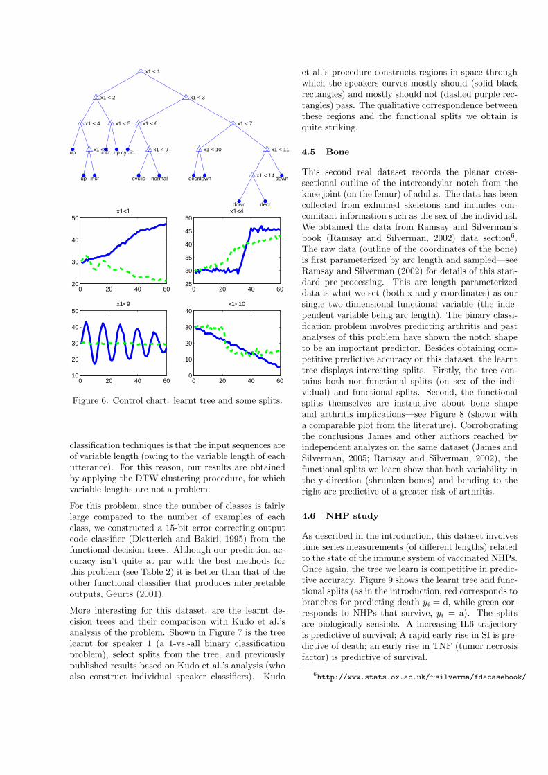
performs best on this dataset, with competitivepredictive accuracy to other techniques (Table 2).Figure 6 shows the complete functional decision treealong with select functional splits. Notice that thehighest level split (x1 < 1) corresponds broadly topartitioning the instances as those that generallyincrease and those that generally decrease (cyclicand normal are arbitrarily assigned to one or other).Appealingly, other internal splits display similar sortsof intuitive behavior (see x1 < 4, for example) andleaf splits display strong representative instances ofthe component classes (see x1 < 9 and x1 < 10).
4.4 Japanese Vowels
Another dataset in the UCI KDD Archive, theJapanese Vowels dataset was first used in Kudo et al.(1999). The classification problem is a speaker identi-fication task and the dataset consists the utterance ofthe Japanese vowels “a” and “e” by nine male speak-ers (yi ∈ {1, . . . , 9}). Each utterance is describedby 12 temporal attributes, which are 12 time-varyingLPC spectrum coefficients (for details of how these at-tributes were obtained see Kudo et al. 1999). An im-portant challenge this dataset poses to many standard
5Hettich and Bay (1999), http://kdd.ics.uci.edu
up incr up cyclic
up incr cyclic normal decrdown down
down decr
x1 < 1
x1 < 2 x1 < 3
x1 < 4 x1 < 5 x1 < 6 x1 < 7
x1 < 8 x1 < 9 x1 < 10 x1 < 11
x1 < 14
0 20 40 6020
30
40
50x1<1
0 20 40 6025
30
35
40
45
50x1<4
0 20 40 6010
20
30
40
50x1<9
0 20 40 600
10
20
30
40x1<10
Figure 6: Control chart: learnt tree and some splits.
classification techniques is that the input sequences areof variable length (owing to the variable length of eachutterance). For this reason, our results are obtainedby applying the DTW clustering procedure, for whichvariable lengths are not a problem.
For this problem, since the number of classes is fairlylarge compared to the number of examples of eachclass, we constructed a 15-bit error correcting outputcode classifier (Dietterich and Bakiri, 1995) from thefunctional decision trees. Although our prediction ac-curacy isn’t quite at par with the best methods forthis problem (see Table 2) it is better than that of theother functional classifier that produces interpretableoutputs, Geurts (2001).
More interesting for this dataset, are the learnt de-cision trees and their comparison with Kudo et al.’sanalysis of the problem. Shown in Figure 7 is the treelearnt for speaker 1 (a 1-vs.-all binary classificationproblem), select splits from the tree, and previouslypublished results based on Kudo et al.’s analysis (whoalso construct individual speaker classifiers). Kudo
et al.’s procedure constructs regions in space throughwhich the speakers curves mostly should (solid blackrectangles) and mostly should not (dashed purple rec-tangles) pass. The qualitative correspondence betweenthese regions and the functional splits we obtain isquite striking.
4.5 Bone
This second real dataset records the planar cross-sectional outline of the intercondylar notch from theknee joint (on the femur) of adults. The data has beencollected from exhumed skeletons and includes con-comitant information such as the sex of the individual.We obtained the data from Ramsay and Silverman’sbook (Ramsay and Silverman, 2002) data section6.The raw data (outline of the coordinates of the bone)is first parameterized by arc length and sampled—seeRamsay and Silverman (2002) for details of this stan-dard pre-processing. This arc length parameterizeddata is what we set (both x and y coordinates) as oursingle two-dimensional functional variable (the inde-pendent variable being arc length). The binary classi-fication problem involves predicting arthritis and pastanalyses of this problem have shown the notch shapeto be an important predictor. Besides obtaining com-petitive predictive accuracy on this dataset, the learnttree displays interesting splits. Firstly, the tree con-tains both non-functional splits (on sex of the indi-vidual) and functional splits. Second, the functionalsplits themselves are instructive about bone shapeand arthritis implications—see Figure 8 (shown witha comparable plot from the literature). Corroboratingthe conclusions James and other authors reached byindependent analyzes on the same dataset (James andSilverman, 2005; Ramsay and Silverman, 2002), thefunctional splits we learn show that both variability inthe y-direction (shrunken bones) and bending to theright are predictive of a greater risk of arthritis.
4.6 NHP study
As described in the introduction, this dataset involvestime series measurements (of different lengths) relatedto the state of the immune system of vaccinated NHPs.Once again, the tree we learn is competitive in predic-tive accuracy. Figure 9 shows the learnt tree and func-tional splits (as in the introduction, red corresponds tobranches for predicting death yi = d, while green cor-responds to NHPs that survive, yi = a). The splitsare biologically sensible. A increasing IL6 trajectoryis predictive of survival; A rapid early rise in SI is pre-dictive of death; an early rise in TNF (tumor necrosisfactor) is predictive of survival.
6http://www.stats.ox.ac.uk/∼silverma/fdacasebook/
Table 2: Predictive Performance—Error RatesData Best LR Seg. Fnl. FDT
CBF 01 2.77 0.5 1.17 0.13D
CBF2 - 5.29 - - 0.25D
CC 0.332 10.33 0.5 2.33 2.0E
JV 3.83 - 3.51 19.4 9.46D
Bone - 21.86 - - 19.79E
NHP - 33.33 - - 26.67E
1: Kadous and Sammut (2005) 2: Geurts and Wehenkel(2005) 3: Kudo et al. (1999) D: DTW clustering, E:
Euclidean clustering.
5 DISCUSSION, FUTURE WORK
In this paper, we presented a simple and effective ex-tension to decision trees that allows them to operateon functional input variables. We presented resultsshowing that these functional decision trees are accu-rate and produce interpretable classifiers.
Many extensions to the basic idea presented here sug-gest themselves; we describe a few. The representa-tive curves can be generated by more sophisticatedclustering algorithms; of particular interest would beones designed for clustering functional curves. For ex-ample, the one proposed by James and Sugar (2003).Also, a range of algorithms from model-based cluster-ing (e.g. HMM based) to non-parametric clustering(e.g. Gaussian processes based clustering methods)might be applied.
Further, one is not limited to decision trees as thebase classifier either. An alternative way to view asingle functional split is that it defines an auxiliaryvariable that may be used in addition to standard fea-tures in any classification algorithm. Multi-way splits,for example, might be particularly powerful featuresin multi-class problems. Finally, predictive accuracycan likely be improved by boosting these functionaldecision trees, a topic we are currently investigating.
Acknowledgements
We thank the US National Science Foundation for fi-nancial support as well as the KD-D group, who sup-ported this work through NSF grant EIA-0087022.
References
L. Breiman, J. H. Friedman, R. A. Olshen, andC. J. Stone. Classification and Regression Trees.Wadsworth International Group., 1984.
T. G. Dietterich and G. Bakiri. Solving multiclasslearning problems via error-correcting output codes.Journal of Artificial Intelligence Research, 2:263 – 286,1995.
A. Genkin, D. D. Lewis, and D. Madi-gan. Large-scale bayesian logisitic regres-sion for text categorization., 2004. URLhttp://www.stat.rutgers.edu/∼madigan/PAPERS/.
P. Geurts. Pattern extraction for time-series clas-sification. In L. de Raedt and A. Siebes, editors,PKDD, LNAI 2168, pages 115 – 127, Freiburg, Sep-tember 2001.
P. Geurts and L. Wehenkel. Segment and combineapproach for non-parametric time-series classification.In PKDD, October 2005.
C. J. A. Gonzalez and J. J. R. Diez. Boosting interval-based literals: Variable length and early classifica-tion. In A. Kandel M. Last and H. Bunke, editors,Data mining in time series databases. World Scien-tific, 2004.
S. Hettich and S. D. Bay. The UCI KDD archive,1999. URL http://kdd.ics.uci.edu.
G. James and B. Silverman. Functional adaptivemodel estimation. Journal of the American StatisticalAssociation, 100:565 – 576, 2005.
G. James and C. Sugar. Clustering for sparsely sam-pled functional data. Journal of the American Statis-tical Association, 98:397 – 408, 2003.
M. W. Kadous and C. Sammut. Classification of mul-tivariate time series and structured data using con-structive induction. Machine Learning Journal, 58:179 – 216, 2005.
M. Kudo, J. Toyama, and M. Shimbo. Multidimen-sional curve classification using passing-through re-gions. Pattern Recognition Letters, 20(11-13):1103 –1111, 1999.
J. R. Quinlan. C4.5: Programs for Machine Learning.Morgan Kaufmann, San Mateo, California, 1993.
J. O. Ramsay and B. W. Silverman. Applied Func-tional Data Analysis: Methods and Case Studies.Springer-Verlag, New York, 2002.
N. Saito. Local feature extraction and its applicationusing a library of bases. PhD thesis, Yale University,1994.
H. Shimodaira, K. i. Noma, M. Nakai, andS. Sagayama. Dynamic time-alignment kernel in sup-port vector machine. In NIPS, volume 2, pages 921 –928, 2001.

0 0
0 0
0 1 1 0
x11 < 1
x4 < 2 x10 < 3
x3 < 4 x1 < 5
x2 < 7 x3 < 8
0 10 20 30−1
0
1
2
3x1<5
0 10 20 30−2
−1
0
1x2<7
0 10 20 30−1
0
1
2x3<4
0 10 20 30−1
−0.5
0
0.5
1x4<2
Figure 7: Japanese Vowels: Functional splits corre-sponding to reported results in Kudo et al. (1999).Branches corresponding to speaker 1 have been col-ored red for ease of comparison. Note: the bottomfigure is a capture of a figure in Kudo et al. (1999).
0 0.2 0.4 0.6 0.8 10
0.1
0.4
0.6
0.8
1x1<1
x
y
0 0.2 0.4 0.6 0.8 10
0.2
0.4
0.6
0.8
1x1<2
x
y
Figure 8: Bone data comparative results. Top Row fig-ures: captures from a figure in James and Silverman(2005). Plot shows, in blue, the first two principalcomponents of the predictive model they propose. ’-’sign curve being for arthritic bones and the ’+’ curvebeing for healthy bone shapes (mean bone shape inred). Lower row figures: root and next level split oflearnt FDT (tree not shown). Branches of the func-tional splits predicting arthritis are colored red.
0 10 20 30 40 500
1
2
3
4x7 < 1, IL6
0 10 20 30 40 500
1
2
3
4x3 < 2, Si
0 10 20 30 40 500.4
0.6
0.8
1
1.2
1.4x9 < 3, TNF
Weeks
a
a
a d
x7 < 1
x3 < 2
x9 < 3
Figure 9: NHP learnt tree, functional splits. Branchesof the functional splits predicting death are coloredred.


![Decision Trees for Hierarchical Multilabel Classification ... · text classification [1] and functional genomics [2]. In functional genomics, an important problem is predicting](https://static.fdocuments.net/doc/165x107/5fb675a0ec941d1cdc0931b7/decision-trees-for-hierarchical-multilabel-classiication-text-classiication.jpg)

![FunSeqSet: Towards a Purely Functional Data Structure for ......Dynamic Trees Problem • We refer to the term “dynamic trees problem” to the one defined by [Sleator and Tarjan,1983]:](https://static.fdocuments.net/doc/165x107/5fa1a7435bc8a5406c4342d3/funseqset-towards-a-purely-functional-data-structure-for-dynamic-trees.jpg)