Decision tree -...
42
Decision Tree LING 572 Fei Xia 1
-
Upload
nguyenkhue -
Category
Documents
-
view
216 -
download
0
Transcript of Decision tree -...

Decision Tree
LING 572
Fei Xia
1
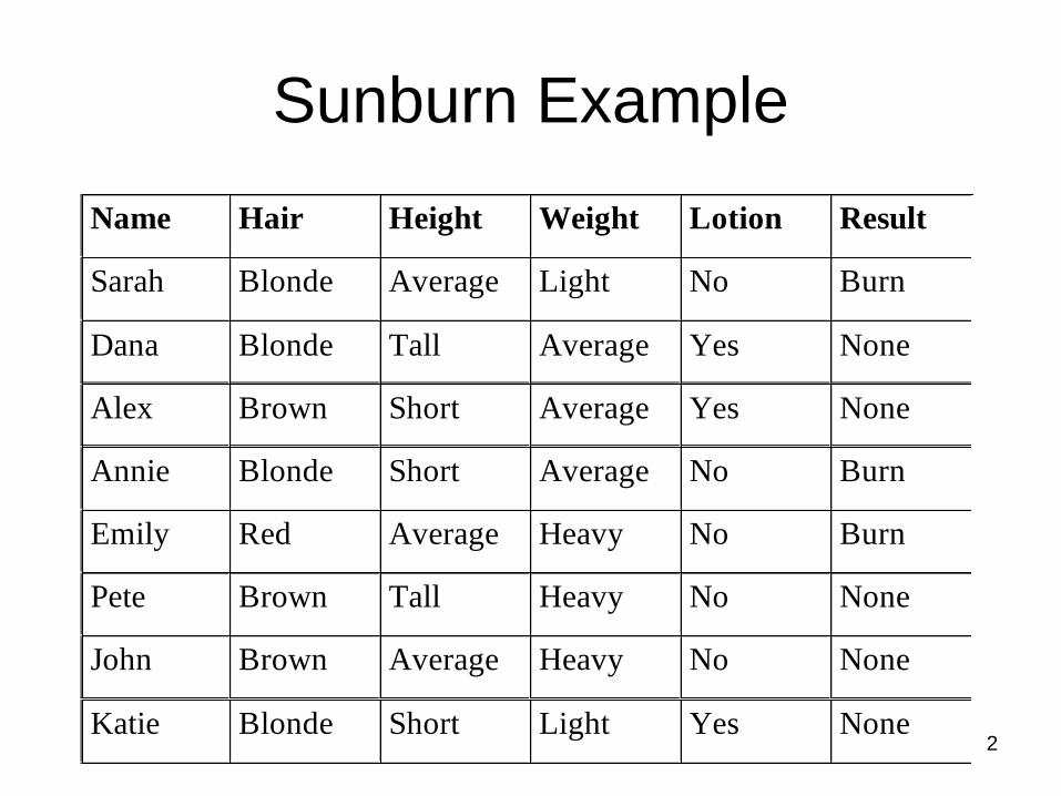
Sunburn Example
Name Hair Height Weight Lotion Result
Sarah Blonde Average Light No Burn
Dana Blonde Tall Average Yes None
Alex Brown Short Average Yes None
Annie Blonde Short Average No Burn
Emily Red Average Heavy No Burn
Pete Brown Tall Heavy No None
John Brown Average Heavy No None
Katie Blonde Short Light Yes None2

Learning about Sunburn
• Goal:
– Train on labelled examples
– Predict Burn/None for new instances
• Solution??
– Exact match: same features, same output
• Problem: N*3*3*3*2 feature combinations, which could
be much worse when there are thousands or even
millions of features.
– Same label as ‘most similar’
• Problem: What’s close? Which features matter? Many
match on two features but differ on result.
3
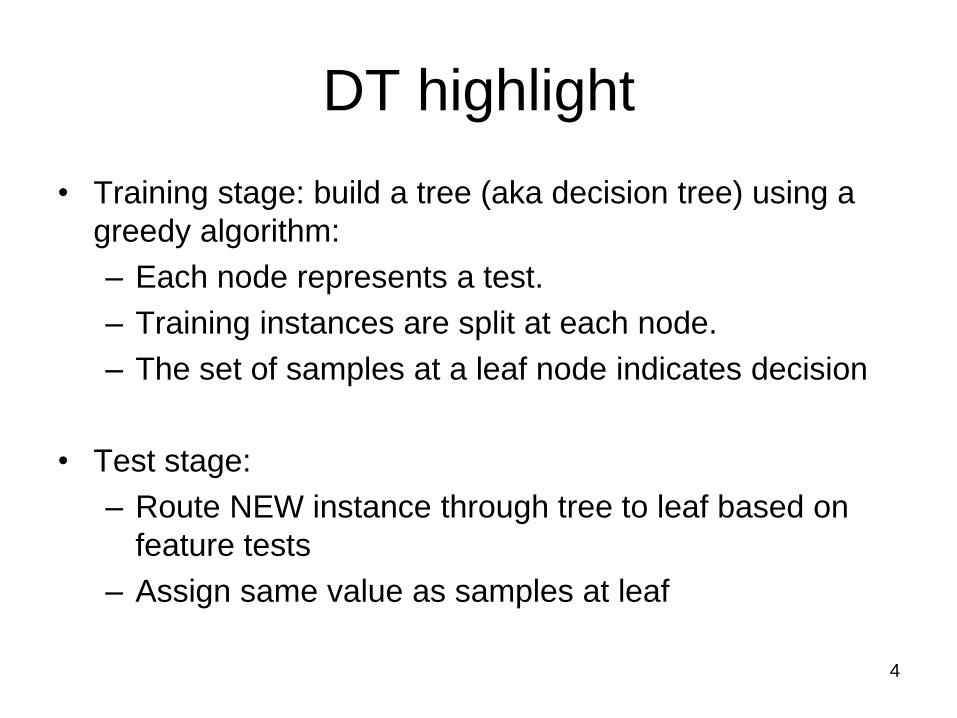
DT highlight
• Training stage: build a tree (aka decision tree) using a
greedy algorithm:
– Each node represents a test.
– Training instances are split at each node.
– The set of samples at a leaf node indicates decision
• Test stage:
– Route NEW instance through tree to leaf based on
feature tests
– Assign same value as samples at leaf
4

Where should we send Ads?
District House
type
Income Previous
Customer
Outcome
(target)
Suburban Detached High No Nothing
Suburban Semi-
detached
High Yes Respond
Rural Semi-
detached
Low No Respond
Urban Detached Low Yes Nothing
…5
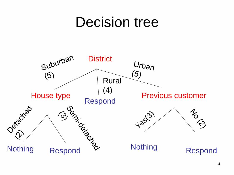
District
Rural
(4)
RespondHouse type
Nothing
Previous customer
RespondNothing
Respond
Decision tree
6

Decision tree representation
• Each internal node is a test:– Theoretically, a node can test multiple features
– In general, a node tests exactly one feature
• Each branch corresponds to test results– A branch corresponds to a feature value or a range of
feature values
• Each leaf node assigns – a class: decision tree
– a real value: regression tree
7

What’s the best decision tree?
• “Best”: We need a bias (e.g., prefer the “smallest” tree):– Smallest depth?
– Fewest nodes?
– Most accurate on unseen data?
• Occam's Razor: we prefer the simplest hypothesis that fits the data.
Find a decision tree that is as small as possible and fits the data
8
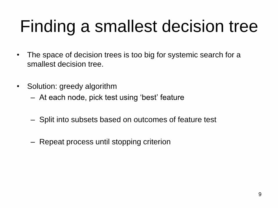
Finding a smallest decision tree
• The space of decision trees is too big for systemic search for a
smallest decision tree.
• Solution: greedy algorithm
– At each node, pick test using ‘best’ feature
– Split into subsets based on outcomes of feature test
– Repeat process until stopping criterion
9

Basic algorithm: top-down induction
1. Find the “best” feature, A, and assign A as the decision
feature for the node
2. For each value (or a range of values) of A, create a
new branch, and divide up training examples
3. Repeat the process 1-2 until the gain is small enough
Effectively creates set of rectangular regions
Repeatedly draws lines in different axes
10

Features in DT
• Pros: Only features with high gains are used as tests
when building DT
irrelevant features are ignored
• Cons: Features are assumed to be independent
if one wants to capture group effect, he must model
that explicitly (e.g., creating tests that look at feature
combinations)
11
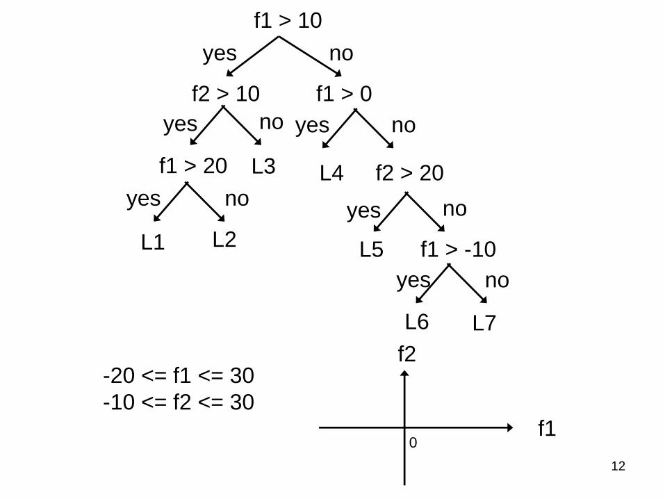
12
f1 > 10
f2 > 10
yes no
f1 > 0
yes no yes no
f1 > 20
yes no
L1 L2
L3 L4 f2 > 20
yes no
L5
yes no
f1 > -10
L6 L7
-20 <= f1 <= 30
-10 <= f2 <= 30
f1
f2
0

Major issues
Q1: Choosing best feature: what quality
measure to use?
Q2: Determining when to stop splitting:
avoid overfitting
Q3: Handling features with continuous
values
13

Q1: What quality measure
• Information gain
• Gain Ratio
• 2
• Mutual information
• ….
14
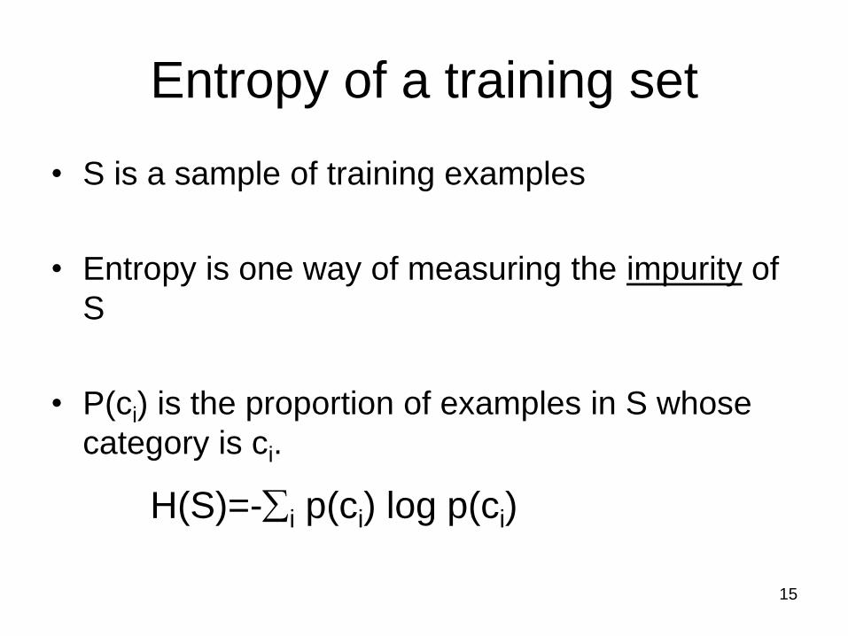
Entropy of a training set
• S is a sample of training examples
• Entropy is one way of measuring the impurity of
S
• P(ci) is the proportion of examples in S whose
category is ci.
H(S)=-i p(ci) log p(ci)
15

Information gain
• InfoGain(Y | X): We must transmit Y. How many
bits on average would it save us if both ends of
the line knew X?
• Definition:
InfoGain (Y | X) = H(Y) – H(Y|X)
• Also written as InfoGain (Y, X)
16

Information Gain
• InfoGain(S, A): expected reduction in entropy due to knowing A.
• Choose the A with the max information gain.
(a.k.a. choose the A with the min average entropy)
)(||
||)(
)|()()(
)|()(),(
)(
a
AValuesa
a
a
SHS
SSH
aASHaApSH
ASHSHASInfoGain
17
Average
Entropy

An example
IncomeHigh Low
S=[9+,5-]
H=0.940
[3+,4-] [6+,1-]
InfoGain (S, Income)
=0.940-(7/14)*0.985-(7/14)*0.592
=0.151
PrevCustom
Yes No
S=[9+,5-]
H=0.940
[6+,2-] [3+,3-]
InfoGain(S, PrevCustom)
=0.940-(8/14)*0.811-(6/14)*1.0
=0.048
H=0.985 H=0.592 H=0.811 H=1.00
18

Other quality measures
• Problem of information gain:
– Information Gain prefers attributes with many values.
• An alternative: Gain Ratio
Where Sa is subset of S for which A has value a.
||
||log
||
||)(),(
),(
),(),(
2
)( S
S
S
SAHASSplitInfo
ASSplitInfo
ASInfoGainASGainRatio
a
AValuesa
aS
19

Q2: Avoiding overfitting
• Overfitting occurs when the model fits the training data too well:
– The model characterizes too much detail or noise in our training data.
– Why is this bad?
• Harms generalization
• Fits training data well, fits new data badly
• Consider error of hypothesis h over
– Training data: ErrorTrain(h)
– Entire distribution D of data: ErrorD(h)
• A hypothesis h overfits training data if there is an alternative hypothesis h’, such that
– ErrorTrain(h) < ErrorTrain(h’), and
– ErrorD(h) > errorD(h’) 20
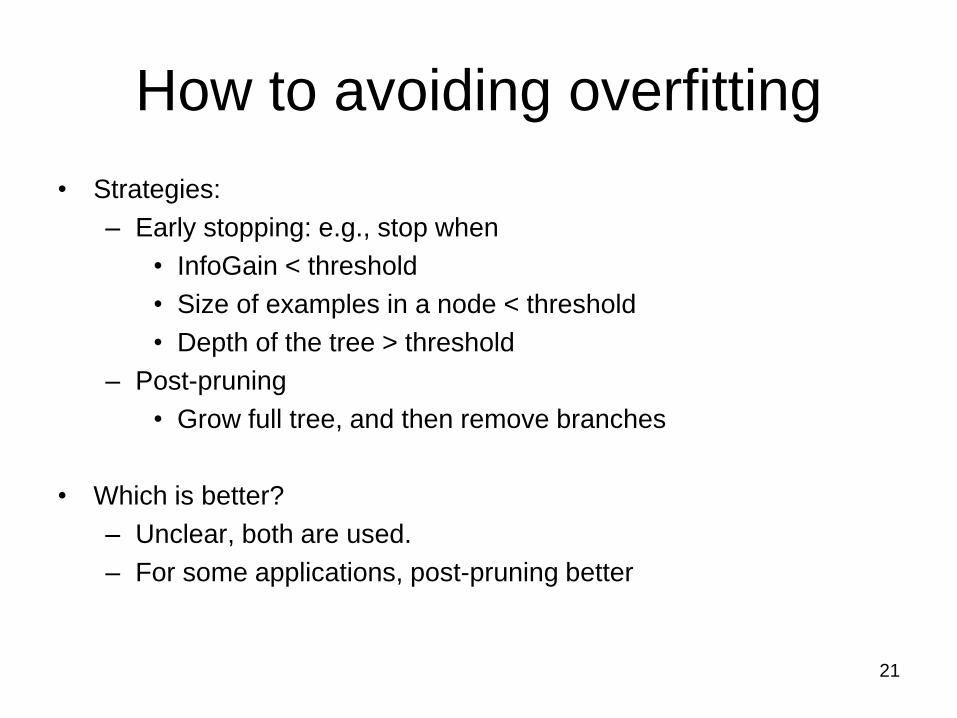
How to avoiding overfitting
• Strategies:
– Early stopping: e.g., stop when
• InfoGain < threshold
• Size of examples in a node < threshold
• Depth of the tree > threshold
– Post-pruning
• Grow full tree, and then remove branches
• Which is better?
– Unclear, both are used.
– For some applications, post-pruning better
21
Post-pruning
• Split data into training and validation sets
• Do until further pruning is harmful:
– Evaluate impact on validation set of pruning each possible node (plus those below it)
– Greedily remove the ones that don’t improve the performance on validation set
Produces a smaller tree with good performance
22
Performance measure
• Accuracy:
– on validation data
– K-fold cross validation
• Misclassification cost: Sometimes more accuracy is desired for some classes than others.
• Minimum description length (MDL): – Favor good accuracy on compact model
– MDL = model_size(tree) + errors(tree)
23

Rule post-pruning
• Convert the tree to an equivalent set of rules
• Prune each rule independently of others
• Sort final rules into a desired sequence for use
• Perhaps most frequently used method (e.g.,
C4.5)
24

District
Rural
(4)
RespondHouse type
Nothing
Previous customer
Respond
Nothing Respond
Decision tree rules
25
If District==Urban && PrevCustomer==Yes then Nothing
Q3: handling numeric features
• Different types of features need different tests:
– Binary: Test branches on true/false
– Discrete: Branches for each discrete value
– Continuous feature discrete feature
• Example
– Original attribute: Temperature = 82.5
– New attribute: (temperature > 72.3) = true, false
Question: how to choose split points?
26
Choosing split points for a
continuous attribute
• Sort the examples according to the values of the continuous attribute.
• Identify adjacent examples that differ in their target labels and attribute values
a set of candidate split points
• Calculate the gain for each split point and choose the one with the highest gain.
27

Summary of Major issues
Q1: Choosing best attribute: different quality
measures.
Q2: Determining when to stop splitting: stop
earlier or post-pruning
Q3: Handling continuous attributes: find the
breakpoints
28
Other issues
Q4: Handling training data with missing
feature values
Q5: Handing features with different costs
– Ex: features are medical test results
Q6: Dealing with y being a continuous value
29

Q4: Unknown attribute values
Possible solutions:
• Assume an attribute can take the value “blank”.
• Assign most common value of A among training data at node n.
• Assign most common value of A among training data at node n which have the same target class.
• Assign prob pi to each possible value vi of A– Assign a fraction (pi) of example to each descendant in tree
– This method is used in C4.5.
30
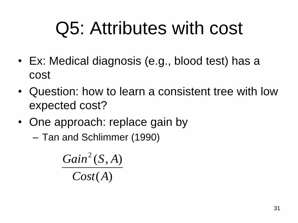
Q5: Attributes with cost
• Ex: Medical diagnosis (e.g., blood test) has a
cost
• Question: how to learn a consistent tree with low
expected cost?
• One approach: replace gain by
– Tan and Schlimmer (1990)
)(
),(2
ACost
ASGain
31

Q6: Dealing with continuous target attribute
Regression tree
• A variant of decision trees
• Estimation problem: approximate real-valued functions: e.g., the crime rate
• A leaf node is marked with a real value or a linear function: e.g., the mean of the target values of the examples at the node.
• Measure of impurity: e.g., variance, standard deviation, …
32

Summary
• Basic case: – Discrete input attributes
– Discrete target attribute
– No missing attribute values
– Same cost for all tests and all kinds of misclassification.
• Extended cases:– Continuous attributes
– Real-valued target attribute
– Some examples miss some attribute values
– Some tests are more expensive than others.
33

Strengths of decision tree
• Simplicity (conceptual)
• Robust to irrelevant features
• Efficiency at testing time
• Interpretability: Ability to generate understandable rules
• Ability to handle both continuous and discrete attributes.
34

Weaknesses of decision tree
• Efficiency at training: sorting, calculating gain, etc.
• Poor feature combination
• Theoretical validity: greedy algorithm, no global optimization
• Predication accuracy: trouble with non-rectangular regions
• Stability: not stable
• Sparse data problem: split data at each node.
35
Addressing the weaknesses
• Used in classifier ensemble algorithms:
– Bagging: sample the training data m times, build a
classifier for each sample, and then let the m
classifiers vote on a test instance.
– Boosting: build one classifier at a time, based on the
results of the current ensemble
• Decision tree stump: one-level DT
36
Common algorithms
• ID3
• C4.5
• CART
More in “additional slides”
37

Additional slides
38

Common algorithms
• ID3
• C4.5
• CART
39

ID3
• Proposed by Quinlan (so is C4.5)
• Can handle basic cases: discrete
attributes, no missing information, etc.
• Information gain as quality measure
40
C4.5
• An extension of ID3:
– Several quality measures
– Incomplete information (missing attribute
values)
– Numerical (continuous) attributes
– Pruning of decision trees
– Rule derivation
– Random mood and batch mood
41
CART
• CART (classification and regression tree)
• Proposed by Breiman et. al. (1984)
• Constant numerical values in leaves
• Variance as measure of impurity
42