- . 1 .

Y

N A S A C O N T R A C T O R R E P O R T

DECISION-MAKING I N A FUZZY ENVIRONMENT

by R. E. Bellman und L. A. Zudeh

$ Prepared by 3 -5 8 UNIVERSITY OF CALIFORNIA ,& 4 Berkeley, Calif. 94720 W! '",, for

N A T I O N A L A E R O N A U T I C S A N D S P A C E A D M I N I S T R A T I O N W A S H I N G T O N , D. C . MAY 1970

https://ntrs.nasa.gov/search.jsp?R=19700017250 2020-05-03T01:45:50+00:00Z

TECH LIBRARY KAFB, NM

C&W'O' J NASA CR-1594

/' DECISION-MAKING IN A FUZZY ENVIRONMENT

J L/

By R. E. Bellman and L. A. Zadeh

, 7 . !, , ..

,i/' .( -. c - " t

Issued by Originator as Report No ERL-69-8 'i

pJ Prepared under Grant No. NGL-05-003-016 by

ELECTRONICS RESEARCH LABORATORY ; J C ~ C , . . iL:L'!4; i<c'L:& / - . UNIVERSITY OF CALIFORNIA I

F b , Ltc, 3' Berkeley, Calif. 94720 J,,i! za",

for

NATIONAL AERONAUTICS AND SPACE ADMINISTRATION

For sale by the Clearinghouse far Federal Scientific and Technical Information Springfield, Virginia 22151 - CFSTI price $3.00

ABSTRACT

By decision-making in a fuzzy environment is meant a

decision process in which the goals and/or the constraints, but not

necessarily the system under control, are fuzzy in nature. This means

that the goals and/or the constraints Constitute classes Of alternatives

whose boundaries are not sharply defined.

An example of a fuzzy constraint is: "The cost of A

should not be substantially higher than a," where a is a specified

constant. Similarly, an example of a fuzzy goal is: "x should be in

the vicinity of x ' I where x is a constant. The underlined words are

the sources of fuzziness in these examples. 0, 0

Fuzzy goals and fuzzy constraints can be defined pre-

cisely as fuzzy sets in the space of alternatives. A fuzzy decision,

then, may be viewed as an intersection of the given goals and con-

straints. A maximizing decision is defined as the set of points in

the space of alternatives at which the membership function of a fuzzy

decision attains its maximum value.

The use of these concepts is illustrated by examples

involving multistage decision processes in which the system under

-iii-

control is either deterministic or stochastic. By using dynamic pro-

gramming, the determination of a maximizing decision is reduced to the

solution of a system of functional equations. A reverse-flow technique

is described for the solution of a functional equation arising in con-

nection with a decision process in which the termination time is defined

implicitly by the condition that the process stops when the system under

control enters a specified set of states in its state space.

- iv-

CONTENTS

1.

2.

3.

4 .

5.

6.

7.

INTRODUCTION

A BRIEF INTRODUCTION TO FUZZY SETS

FUZZY GOALS, CONSTRAINTS AND DECISIONS

MULTISTAGE DECISION PROCESSES

STOCHASTIC SYSTEMS IN A FUZZY ENVIRONMENT

SYSTEMS WITH IMPLICITLY DEFINED TERMINATION TIME

CONCLUDING REMARKS

REFERENCES

FIGURES

Page No.

1

5

15

25

31

36

51

53

-V-

1. INTRODUCTION

Much of the decision-making in the real world takes place

in an environment in which the goals, the constraints and the conse-

quences of possible actions are not known precisely. To deal quantita-

tively with imprecision, we usually employ the concepts and techniques of

probability theory and, more particularly, the tools provided by decisSon

theory, control theory and information theory. In so doing, we are tac-

itly accepting the premise that imprecision - whatever its nature - c.an be equated with randomness. This, in our v+ew, is a questionable as-

sump t ion.

Specifically, our contention is that there is a need for

differentiation between randomness and fuzziness, with’ the latter being

a major source of imprecision in many decision processes. By fuzziness,

we mean a type of imprecision which is associated with the use of fuzzy

sets,’”that is, classes in which there is no sharp transition from

membership to non-membership. For example, the class of green objects

is a fuzzy set. So are the classes of objects characterized by such

commonly used adjectives as large, small, substantial, significant,

important, serious, simple, accurate, approximate, etc. Actually, in

sharp contrast to the notion of a class or a set in mathematics, most of

the classes in the real world do not have crisp boundaries which separate

those objects which belong to the classes in question from those which

do not. In this connection, it is important to note that, in the dis-

course between humans, statements such as “John is several inches taller

.

than Jim," "x is much larger than y, "Corporation X has a bright

future, "the stock market has suffered a sharp decline, convey inf or-

matlon despite the fuzziness of the meaning of the underlined words. In

fact, it may be argued that the main distinction between human intel-

ligence and machine inte1,ligence lies in the ability of humans -- an ability which present-day computers do not possess -- to manipulate fuzzy concepts and respond to fuzzy instructions.

What is the distinction between randomness and fuzziness?

Essentially, randomness has to do with unkertainty concerning membership

or non-membership of an object in a non-fuzzy set. Fuzziness, on the

other hand, has to do with classes in which there may be grades of mem-

bership intermediate between full membership and non-membership. To

illustrate the point, the fuzzy assertion "Corporation X has a modern

outlook" is imprecise by virtue of the fuzziness of the terms "modern

outlook." On the other hand, the statement "The probability that Cor-

poration X is operating at a loss is 0.8," is a measure of the uncer-

tainty concerning the membership of Corporation X in the non-fuzzy class

of corporations which are operating at a loss.

Reflecting this distinction, the mathematical techniques

for dealing with fuzziness are quite different from those of probability

theory. They are simpler in many ways because to the notion of prob-

ability measure in probability theory corresponds the simpler notion of

membership function in the theory of fuzziness. Furthermore, the cor-

2

respondents of a + b and ab, where a and b are real numbers, are the simpler operations Max(a,b) and Min(a,b). For this reason, even in

those cases in which fuzziness in a decision process can be simulated by

a probabilistic model, it is generally advantageous to deal with it

through the techniques provided by the theory of fuzzy sets rather than

through the employment of the conceptual framework of probability theory.

Decision processes in which fuzziness enters in one way

or another’can be studied from many points of view. 3’4 ’5 In the present

note, our main concern is with introducing three basic concepts: fuzzy

goal, fuzzy constraint and fuzzy decision, and exploring the application

of these concepts to multistage decision processes in which the goals or

the constraints may be fuzzy, while the system under control may be either

deterministic or stochastic - but not fuzzy. This, however, is not an intrinsic restriction on the applicability of the concepts and techniques

described in the following sections.

Roughly speaking, by a fuzzy goal we mean an objective

which can be characterized as a fuzzy set in an appropriate space. To

illustrate, a simple example of a fuzzy goal involving a real-valued

variable x would be: “x should be substantially larger than 100.”

Similarly, a simple example of a fuzzy constraint would be: “x should

be approximately in the range 20-25.’’ The sources of fuzziness in these

statements are the underlined words.

3

A less trivial example is provided by a deterministic

discrete-time system characterized by the state equations

xn+l = xn + un , n=0,1,2,. . . where x and u denote, respectively, the state and input at time n and

in which for simplicity xn and un are assumed to be real-valued. Here

a fuzzy constraint on the input may be

n n

where the wavy bar under a symbol plays the role of a fuzzifier, that is,

a transformation which takes a non-fuzzy set into a fuzzy set which is

approximately equal to it. In this instance, u < 1, would read "un

should be approximately less than or equal to 1, and the effect of the

fuzzifier is to transform the non-fuzzy set - 1 < u < 1 into a fuzzy set

-1 - un 5 1. The way in which the latter set can be given a precise mean-

n:

- n - w u

ing will be discussed in Section 2.

Assume that the fuzzy goal is to make x approximately 3 equal to 5, starcing with the initial state x. = 1. Then, the problem is

to find a sequence of inputs u ul, u2 which will realize the specified

goal as nearly as possible, subject to the specified constraints on u 0'

0' ul,

In what follows, we shall consider in greater detail a few

representative problems of this type. It should be stressed that our

limited objective in the present paper is to draw attention to problems

involving multistage decision processes in a fuzzy environment and

4

suggest tentative ways of attacking them, rather than to develop a gen-

eral theory of decision processes in which fuzziness and randomness may

enter.in a variety of ways and combinations. In particular, we shall not

concern ourselves with the application to decision-making of the concept

of a fuzzy algorithm3 - a concept which may be of use in problems which are less susceptible to quantitat'ive analysis than those considered in

the sequel.

For convenience of the reader, a brief summary of the

basic properties of fuzzy sets is provided in the following section.

"" ~ .. . ~- ~~~ ~~

2. A Brief Introduction to Fuzzy Sets

Informally, a fuzzy set is a class of objects in which

there is no sharp boundary between those objects that belong to the class

and those that do not. A more precise definition may be stated as fol-

lows.

Definition. Let X = (x} denote a collection of objects (points) denoted

generically by x. Than a fuzzy set A X is a set of ordered pairs

A = {(x,pA(x))} , x E X (1)

where p (x) is termed the grade of membership of x A, and vA: X +. M

is a function from X to a space M called the membership space. When M

contains only two points, 0 and 1, A is non-fuzzy and its membership

A

5

function becomes identical with the characteristic function of a non-

fuzzy set.

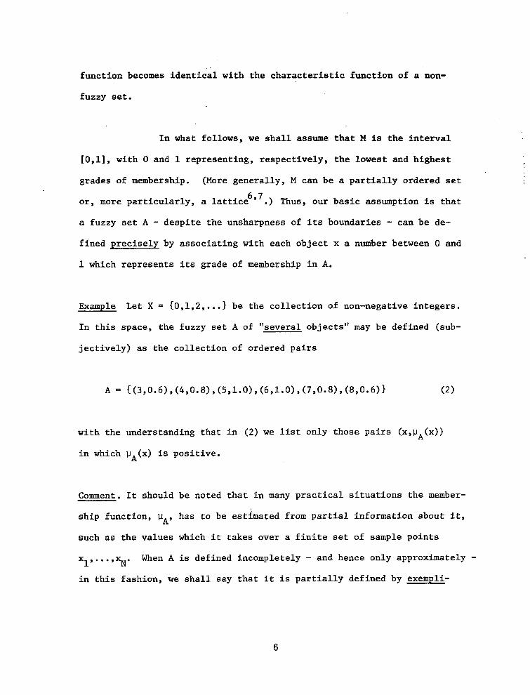
In what follows, we shall assume that M is the interval

[0,1], with 0 and 1 representing, respectively, the lowest and highest

grades of membership. (More generally, M can be a partially ordered set

or, more particularly, a lattice6” .) Thus, our basic assumption is that a fuzzy set A - despite the unsharpness of its boundaries - can be de- fined precisely by associating with each object x a number between 0 and

1 which represents its grade of membership in A.

Example Let X = (0,1,2,. . . I be the collection of non-negative integers.

In this space, the fuzzy set A of “several objects” may be defined (sub-

jectively) as the collection of ordered pairs

A = {(3,0.6) , (4,0.8), (5,1.0), (6,1.0), (7,0.8), (8,0.6)) (2)

with the understanding that in ( 2 ) we list only those pairs (x,v (x))

in which LI (x) is positive.

A

A

Comment, It should be noted that in many practical situations the member-

ship function, LIAy has to be estimated from partial information about it,

such as the values which it takes over a finite set of sample points

xl, ...,%. When A is defined incompletely - and hence only approximately - in this fashion, we shall say that it is partially defined by exempli-

\

6

f ication. The problem of estimating pA from. the. knowledge of the set of

pairs (xl,pA(xl)) , .. . (%,pA(%)) is the problem of abstraction - a prob- lem that plays a central role in pattern recognition. ” We shall not

concern ourselves with the solution of this problem in the present

paper and will assume throughout - except where explicitly stated to the contrary - that p (x) is given for all x in X. A

For notational purposes, it is convenient to have a de-

vice for indicating that a fuzzy set A .is obtained from a non-fuzzy set

by fuzzifying the boundaries of the latter set. For this purpose, we

shall employ a wavy bar under a symbol (or symbols) which define x. For

example, if A is the set .of real numbers between 2 and 5, i.e., x = {x I 2 < x < 5}, then A = (x I 2 < X 5 5) is a fuzzy set of real numbers which

are approximately between 2 and 5. Similakly, A = {x I x = - 5) or simply 5 will denote the set of numbers which are approximately equal to 5 . The

symbol - will be referred to as a fuzzifier.

” - “3

...

We turn next to the definition of several basic concepts

which we shall need in later sections.

Normality: A fuzzy set A is normal if and only if Sup pA(x) = 1, that is,

the supremum of vA(x) over X is unity. A fuzzy set is subnormal if it is

not normal. A non-empty subnormal fuzzy set can be normalized by

dividing each pA(x) by the factor S;p pA(x). (A fuzzy set A is empty if

and only if p,(x) i 0. )

x

7

Equality: Two fuzzy sets are equal, written as A = B, if and only if

- VA - VB, that is, vA(x) = pB(x) for all x in X. (In the sequel, to

simplify the notation we shall omit the argument x when an equality or

inequality holds for all values of x in X.)

Containment: A fuzzy set A is contained or is a subset of a fuzzy set

B, written as A C B , if and only if 1-I < PB. In this sense, the fuzzy Eat

of very large numbers is a subset of the fuzzy set of large numbers.

A -

Complementation: A' is said to be the complement of A if and only if

PA' = - pA. For example, the fuzzy sets: A =' {tall men} and A' =

{not tall men) are complements of one another if the negation "not" is

interpreted as an operation which replaces 1-1 (x) with l-vA(x) for each

x in X.

A

Intersection: The intersection of A and B is denoted by A n B and is de-

fined as the largest fuzzy set contained in both A and B. The membership

function of A rl B is given by

where Min(a,b) = a if azb and Min(a,b) = b if a>b. In infix form, using

the conjunction symbol A in place of Min,(3) can be written more simply as

a

The not ion of i n t e r sec t ion bea r s a close r e l a t i o n t o t h e

not ion of the connective "and." Thus, i f A is t h e class of t a l l men and

B is the class of f a t men9 then A n B i s the class of men who are both t a l l

and fat . -

Comment, It should be noted. that our ident i f icat ion of "and" with (4)

imp l i e s t h a t we are i n t e r p r e t i n g "and" i n a "hard" sense, that is, we do

not a l low any tradeoff between p (x) and p (x) so long as p (x) > ~ . l ' (x).

For example, i f pA(x) = 0.8 and pB(x) = 0.!j9 then pA n ,(x) = 0.5 so long

as pA(x) 0.5. I n some cases, a s o f t e r i n t e r p r e t a t i o n of "and'! vhich

corresponds to forming the a lgebraic product of pA(x) and pB(x) - r a t h e r

than the conjunct ion 1-1 (x) A 1-1 (x) - may be c lose r t o t he i n t ended mean-

ing of "and." From the mathematical as well as p rac t i ca l po in t s o f view,

the i den t i f i ca t ion o f "and" with A is p re fe rab le t o its i d e n t i f i c a t i o n

A B A B

A B

with the product, except where A clear ly does not express the sense i n

which one wants "and" t o b e i n t e r p r e t e d . F o r t h i s r e a s o n , i n t h a t f o l -

10~7s "and" will be understood to be a hard "and" u n l e s s e x p l i c i t l y s t a t e d

t h a t i t should be interpreted as a s o f t "and"(in the s ense of corre-

sponding to t he a lgeb ra i c p roduc t of membership func t ions) .

Union: The not ion of the union of A of B is dua l t o t he no t ion of i n t e r -

sec t ion . Thus, the union of A and B, denoted as A u B , i s def ined as t h e

smallest fuzzy set containing both A and B. The membership function of

A u B is given by

9

where Max (a,b) = a if a b and Max (a,b) = b if a < b. In infix form,

using the disjunction symbol vein place of Max, we can write (5) more

simply as

As in the case of the intersection, the union of A and B

bears a close relation to the connective "or. Thus, if A = (tall men)

and B = (fat men), then A u B = (tall or fat men}. Also, we can differen-

tiate between a hard "or:'1, which corresponds to (6) , and a soft "or",

which corresponds to the algebraic of A and B, which is denoted by

A e B and is defined by (9).

It is easy to verify that u and are related to one

another by the identity

Algebraic product: The algebraic product of A and B is denoted by A3 and

is defined by

Algebraic sum: The algebraic of A and B is denoted by A +3 B and is

defined by

10

It is easy to verify that

1

A 0 B = (A'B')

Comment. .It should be noted that the operations v and II are associative

and distributiverover one$nother. on the other hand, e (product) and +3 (sum) are

associative but not distributive,

Convexity and concavity. Let A be a fuzzy set in X = R". Then A is

convex if and only If f o r every pair of points (x,y) i n X, the membership

. for 0 X 51. Dually, A is concave if its complement A' is convex. It

I s easy to show that if A and B are convex, so is A!%. Dually, if A and

B are concave, so is A m ,

Relation. A fuzzy relation, R, in the product space XxY = { (x,y) 1, x E X,

y E Y, is a fuzzy set i n X x Y characterized by a membership function %

which associates with each ordered pair (x,y) a grade of membership

pR(x,y) in R. More generally, an n-ary fuzzy relation in a product space

11

x = x X X X.. . .xx" is a fuzzy set in X characterized by an n-variate membership function %(x1, . . ., x,), xi E X , i = 1, . . ., n.

1 2

i

Example. Let X = Y = R1, where R is the real line (-my ). Then x>>y is a fuzzy relation in R . A subjective expression for % in this case might be: %(x,y) = 0 for x<y; uR(x,y) = (1+ (x-y) ) for x>y.

1

2

-2 -1 -

Fuzzy sets induced by mappings. Let f :X+Y be a mapping from X = {x) to

Y = cy), with the image of x under f denoted by y = f (x). Let A be a

fuzzy set in X. Then, the mapping f induces a fuzzy set B in Y whose

membership function is given by

where the supremum is taken over the set of points f (y) in X which are

mapped by f into y.

-1

Conditioned fuzzy sets: A fuzzy set B(x) in Y = cy) is conditioned on x

if its membership function depends on x as a parameter. This dependence

is expressed by uB(ylx) .

Suppose that the parameter x ranges over a space X, so

that to each x in X corresponds a fuzzy set B ( x ) in Y. Thus, we have a

mapping - characterized by pB (y Ix) - from X to the space of fuzzy sets

12

i n Y. Through t h i s mapping, any given fuzzy set A i n -X induces a ' fuzzy

set B i n Y which is defined by

where ll and y denote the membership func t ions of A and B, respec t ive ly .

In terms of A and v (13) may be wr i t t en more simply as

A B

Note t h a t this equation is analogous - but no t equiva len t - t o t h e ex-

p res s ion fo r t he marg ina l p robab i l i t y d i s t r ibu t ion of t h e j o i n t d i s t r i b -

t i o n of two random variables , wi th pB(y ]x) playing a role analogous to

t h a t of a cond i t iona l d i s t r ibu t ion .

Decomposability: L e t X = {x), Y = {y) and l e t C be a fuzzy set i n t h e

product space Z = XxY defined by a membership function yc(x,y). Then C

is decomposable a long X and Y i f and only i f C admits of the represen-

t a t i o n

c = A ~ B

or equiva len t ly

where A and B are fuzzy sets with membership funct ions of the form

pA(x) and pg(y) , respect ively. (Thus, A and B are cyl indr ica l fuzzy

sets i n Z.) The same ho lds fo r a fuzzy set i n t h e p r o d u c t of any f i n i t e

number of spaces.

Probabi l i ty of fuzzy events: L e t P be a p robab i l i t y measure on Rn. A

fuzzy eventlo A i n Rn is def ined to be a fuzzy subset A of Rn whose mem-

bership function, llA, is measurable. Then, t h e p r o b a b i l i t y of A is de-

f ined by the Lebesgue-St ie l t j es i n t e g r a l

Equivalently,

where E denotes the expectation operator. In the case of a non-fuzzy set ,

(16) reduces to the convent iona l def in i t ion of the p robabi l i ty o f a non-

fuzzy event.

This concludes our brief introduction to some of the bas ic

concepts re la t ing to fuzzy sets. In the fo l lowing sec t ion , we s h a l l u s e

these concepts as a bas i s fo r de f in ing t he cen t r a l no t ions of goal , con-

s t r a i n t and d e c i s i o n i n a fuzzy environment.

14

3. Fuzzy Goals,'Constraints and Decisions

In the conventional approach to decision-making, the

principal ingredients of a decision process are (a) A set of alterna-

tives; (b) a set of constraints on the choice between different alter-

natives; and (c) a performance function which associates with each

alternative the gain (or loss) resulting from the choice of that alter-

native .

When t7e view a decision process from the broader perspec-

tive of decision-making in a fuzzy environment, a different and perhaps

more natural conceptual framework suggests itself. The most important

Eeature of this framework is its symmetry with respect to goals and

constraints - a symmetry, which erases the differences between them and makes it possible to relate in a relatively simple way the concept of a

decision to those of the goals and constraints of a decision process.

r

More specifically, let X = {x) be a given set of alterna-

tives. Then, a fuzzy goal or simply a &, G, in X will be identified

with a given fuzzy set G in X. For exampleg if X = R' (the real line),

then the fuzzy goal expressed in words as I' x should be substantially

larger than 10" might be represented by a fuzzy set in R whose member-

ship function is (subjectively) given by

1

I

PG(X) = 0 , x<10

15

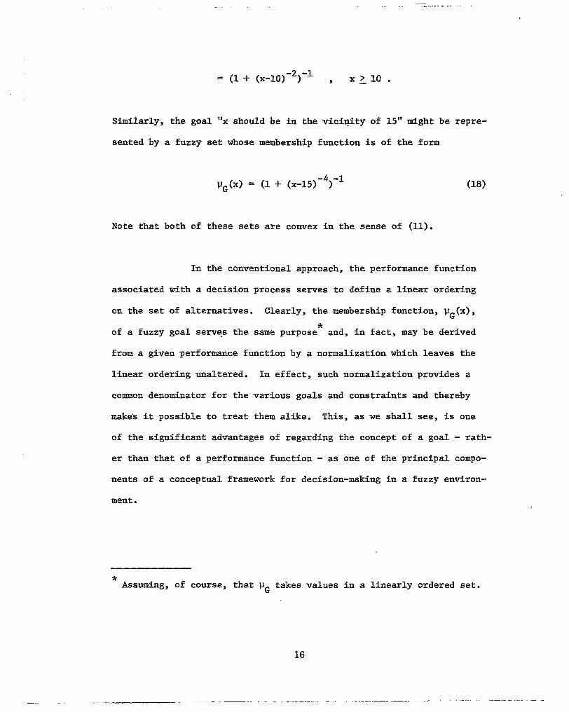
= (1 + (x-10) ) , X L l O . -2 -1

Similarly, the goal "x should be in the vicinity of 15" might be repre-

sented by a fuzzy set whose membership function is of the form

Note that both of these sets are convex in the sense of (11).

In the conventional approach, the performance function

associated with a decision process serves to define a linear ordering

on the set of alternatives. Clearly, the membership function, pG(x),

of a fuzzy goal serves the same purpose and, in fact, may be derived

from a given performance function by a normalization which leaves the

linear ordering unaltered. In effect, such normalization provides a

common denominator f o r the various goals and constraints and thereby

make's it possible to treat them alike. This, as we shall see, is one

of the significant advantages of regarding the concept of a goal - rath- er than that of a performance function - as one of the principal compo- nents of a conceptual framework for decision-making i n a fuzzy environ-

ment.

*

* Assuming, of course, that p takes values in a linearly ordered set. G

T - I'.

In a similar manner, a fuzzy constraint or simply a

constraint, C, in X is defined to be a fuzzy set in X. For example, in

R , the constraint "x should be approximately between 2 and lo," could

be represented by a fuzzy set whose membership function might be of the

f o m

1

where a is a positive number and m is a posftive even integer chosen in

such a way as to reflect the sense in which the approximation to the in-

terval [2,10] is to be understood. For example, if we set m = 4 and a =

5-4, then at x = 2 and x = 10 we have approximately 1~ (x) = 0.8, while

at x = 1 and x = 11, IJ (x) = 0.5; and at x = 0 and x = 12, uc(x) is ap-

proximately equal to 0 . 3 .

C

C

An important aspect of the above definitions of the con-

cepts of goal and constraint is that both are defined as fuzzy sets in

the space of alternatives and thus, as will be elaborated upon below,

can be treated identically in the formulation of a decision. By con-

trast, in the conventional approach to decision-making, a constraint

set is taken to be a non-fuzzy set in the space of alternatives X, where-

as a performance function is a function from X to some other space.

Nevertheless, even in the case of the conventional approach, the use of

Lagrangian multipliers and penalty functions makes it apparent that

there is an intrinsic similarity between performance functions and con-

17

straints. This similarity - indeed identity - is made explicit in our *

formulation, I

As an illustration, suppose that we have a fuzzy goal G

and a fuzzy constraint C expressed as follows:

G: x should be substantially larger than 10, with pG(x)

given by (17)

c : x should be in the viclnity of 15, with p (X) ex- C

pressed by (18).

Note that G and C are connected to one another by the

connective e. Now, as was pointed out in Sec.2, corresponds to the intersection of fuzzy sets. This implies that in the example under

consideration the combined effect of the fuzzy goal G and the fuzzy

constraint C on the choice of alternatives may be represented by the

intersection G n C . The membership -function of the intersection is given

by

or more explicitly

(x) = Min ((1 + (x-10) ) , (1 + (x - 15) ) ) for x > 10 -2 -1 -4 -1 l’lGr?C: -

*For a very thorough discussion of these points see Ref. 12.

18

Note that G n C is a convex fuzzy set since both G and C are convex

fuzzy sets.

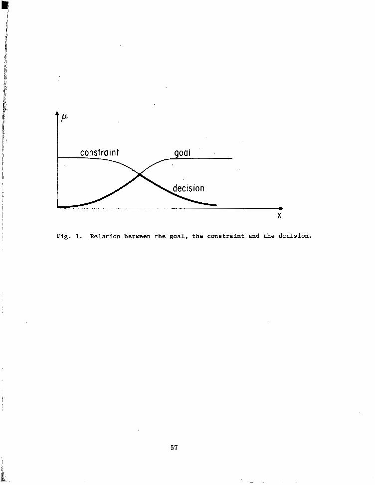
Turning to the concept of a decision, we observe that,

intuitively, a decision is basically a choice or a set of choices drawn

from the available alternatives. The preceding example suggests that a

fuzzy decision or simply a decision be defined as the fuzzy set of alter-

natives resulting from the intersection of the goals and constraints.

We formalize this idea in the following definition.

Definition. Assume that we are given a fuzzy goal G and a fuzzy con-

straint C in a space of alternatives X. Then, G and C combine to form a

decision, D, which is a fuzzy set resulting from intersection of G and C.

In symbols,

D = G n C

and correspondingly

Lf) = ?JG A PC

The relation between G, C and D is depicted in Fig.1.

19

More generally, suppose that we have n goals G 190.09 G n and m constraints C 190.e3 Cm. Then, the resultant decision is the inter-

section of the given goals G ~ 9 ~ ~ ~ 9 G and the given constraints C1OO..s n Cm. That is,

D = ~~n G~ n... n G n cp c2n o o o n cm n

and correspondingly

Note that in the above definition of a decision, the

goals and the constraints enter into the expression for D in exactly

the same way. This is the basis for our earlier statement concerning

the identity of.the roles of goals and constraints in our formulation

of decision processes in a fuzzy environment.

Coment. The definition of a decision as the intersection of the goals

and constraints, reflects our interpretation of "and" in the "hard"

sense of (4) If the interpretation of "and" is left open, we shall

say that a decision - viewed as a fuzzy set - is a confluence of the goals and the constraints. Thus, "confluence" acquires the meaning of

"intersection" when "and" is interpreted in the sense of (4); the mean-

ing of "algebraic product" when "and" is interpreted in the sense of

20

(8); and may be assigned other concrete meanings when a need f o r a spe-

c i a l i n t e r p r e t a t i o n of "and" arises. I n s h o r t , a broad def in i t ion of the

concept of decis ion may be s ta ted as:

Decision = Confluence of Goals and Constraints

As an i l lus t ra t ion o f (21) ' we sha l l cons ider a very

simple example i n which X = €1'2 $ o . ,101 and G19 G2, C and C2 are de-

f ined below.

l

2 3 4 5 6 7 8 9 10

0.1

0.6

0.6

0.4

0.4

1.0

0.9

0.6

0.8

0.9

1.0

0.7

1.0

0.8

0.8

0.9

0.7

0.6

0.7

1.0

0.4 0.2

0.5 0.3

0.5 0.3

0.8 0.6

0

0

0.2

0.4

0

0

0.1

0 .'2

Forming the conjunction of p G1 $ 'G2 ' 'C1 and pc we obta in the

2 fol lowing table of values for pD (x)

X I 1 2 3 4 5 6 7 8 9 10

0 0.1 0.4 0.7 0.8 0.6 0.4 0.2 0 0

Thus the d e c i s i o n i n t h i s c a s e is the fuzzy set

D = {(2,O.1),(3,O.4),(4,O.7)9.(5,O.8)9(6yO~6)y(7,O~4)~(8,O~2~~

21

I

Note that no x in X has full (that is, unity grade) membership in D.

This reflects, of course, the fact that the specified goals and con-

straints conflict with one another, ruling out the existence of an

alternative which fully satisfies all of them.

The concept of a decision as a fuzzy set in the space of

alternatives may appear at first to be somewhat artificial. In fact it

is quite natural, since a fuzzy decision may be viewed as an instruction

whose fuzziness is a consequence of the imprecision of the given goals

and constraints. Thus, in our example, G1, G2, C and C may be respec-

tively expressed in words as: ''x should be close to 5," "x should be 1 2

close to 3 ," "x should be close to 4" and "x should be close to 6 " . The

decision, then, is to choose x to be close to 5. The exact meaning of

11 close" in each case is given by the values of the corresponding member-

ship function.

How should a fuzzy instruction such as "x should be close

to 5" be executed? Although there does not appear to be a universally

valid answer to questions of this type, it is reasonable in many in-

stances to choose that x or x's which have maximal grade of membership

in D. In the case of our example, this would be x = 5.

*

* The execution of fuzzy instructions is discussed in Ref. 3 .

22

More generally, let D be a fuzzy decision and let D be M

its core, that is, the non-fuzzy set of points in X at which the maximum

of pD(x) over X, if it exists, is attained. Then, we shall say that any

x in DM constitutes a maximizing decision. In other words, a maximizing

decision is simply any alternative in X which maximizes pD(x), e.g., x = 5

in the foregoing example. Note that in Rn a sufficient condition for the

-

uniqueness of a maximizing decision is that D be a strongly convex fuzzy

set. *

In defining a fuzzy decision D as the intersection - or more generally, as the confluence - of the goals and constraints, we are tacitly assuming that all of the goals and constraints that enter into

D are, in a sense, of equal importance. These are some situations, how-

ever, in which some of the goals and perhaps some of the constraints are

of greater importance than others. In such cases, D might be expressed

as a convex combination of the goals and the constraints, with the

weighting coefficients reflecting the relative importance of the con-

stituent terms. More explicitly, we may express 1-1 (x) as D

n m

* A fuzzy set is strongly convex if it is convex and its membership function is unimodal.

23

where the Q and 8 . are membership functions such that i J

n m

i=1 j =1 x . Qi(X) + c Bj(X) = 1

Subject to this constraint, then, the values of a (x) and 8 . (x) can be

chosen in such a way as to reflect the relative importance of G1, ..., G and C1, ..., C In particular, if m = n = 1, it is easy to verify that

(22) can generate any fuzzy set which is contained in G u C and contains GnC. Note that (22) resembles the familiar artifice of transforming a

vector-valued criterion into a scalar-valued criterion by forming a linear

combination of the components of the vector-valued objective function.

i J

n

m'

So far, we have restricted our attention to situations in

which the goals and the constraints are fuzzy sets in X, the space of

alternatives. A more general case which is of practical interest is one

in which the goals and the constraints are fuzzy sets in different

spaces. Specifically, let f be a mapping from X = {x) to Y = {y), with

x representing an input (cause) and y, y = f(x), representing the corre-

sponding output (effect).

Suppose that the goals are defined as fuzzy sets G 1'""' G in Y while the constraints C1, ..., C are defined as fuzzy sets in X.

Now, given a fuzzy set G in Y, one can readily find a fuzzy set G in n m *

i i

24

X which induces Gi in Y. Specifically, the membership function of Gi *

is given by the equality

, i = l,...,n

The decision D; then, can be expressed as the intersection

of G1 , . . . ,G and C1,. . . , C Using (23), we can express 1-1 (x) more ex- n m* D plicitly as

* *

where f: X-tY. In this way, the case where the goals and the constraints

are defined as fuzzy sets in different spaces can be reduced to the case

where they are defined in the same space. We shall find ( 2 4 ) of use in

the analysis of multistage decision processes in the following section.

4 . i Multistage .- ~ ~ Decision Processes

As an application of the concepts introduced in the pre-

ceding sections, we shall consider a few basic types of problems involv-

ing multistage decision-making in a fuzzy environment. It should be

stressed that, in what follows, our main purpose is to illustrate the use

of the concepts of fuzzy goal, fuzzy constraint and fuzzy decision, rather

than to develop a general theory of multistage decision processes in

25

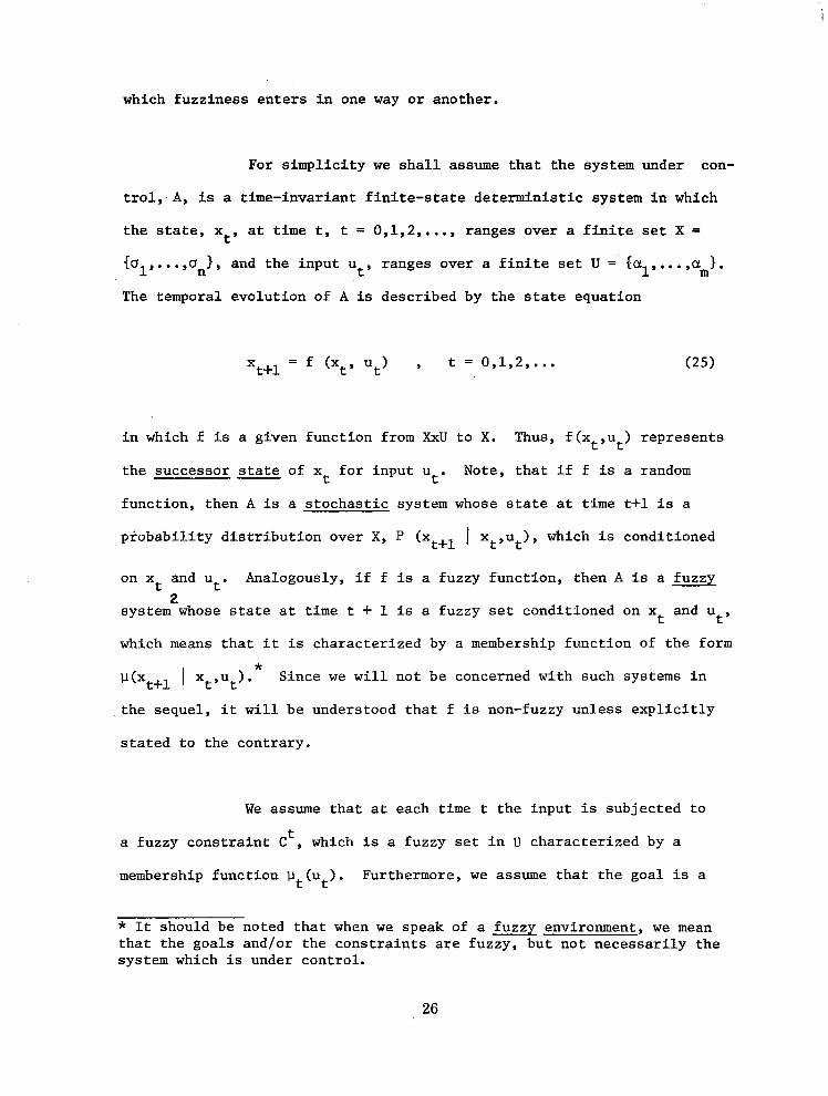
which fuzziness enters in one way or another.

For simplicity we shall assume that the system under con-

trol, A, is a time-invariant finite-state deterministic system in which

the state, x at time t, t = 0,1,2,..., ranges over a finite set X =

{o1,.. .,u 1 , and the input ut, ranges over a finite set U = {al,.. . ,a 1 .

The temporal evolution of A is described by the state equation

ty

n m

x = f (xt, Ut) , t = 0,1,2,. . . t+l (25)

in which f is a given function from XxU to X. Thus, f(x u ) represents t' t

the successor state of x for input u Note, that if f is a random

function, then A is a stochastic system whose state at time t+l is a

probability distribution over X, P ( x ~ + ~ u ), which is conditioned

t t'

I Xt, t on x and u Analogously, if f is a fuzzy function, then A is a fuzzy

system whose state at time t + 1 is a fuzzy set conditioned on x and u t ty

which means that it is characterized by a membership function of the form

~ ( x ~ + ~ I xt,ut). Since we will not be concerned with such systems in the sequel, it will be understood that f is non-fuzzy unless explicitly

t t' 2

*

stated to the contrary.

We assume that at each time t the input is subjected to

a fuzzy constraint Ct , which is a fuzzy set in U characterized by a

membership function 1-1 (u ). Furthermore, we assume that the goal is a t t

* It should be noted that when we speak of a fuzzy environment, we mean that the goals and/or the constraints are fuzzy, but not necessarily the system which is under control.

26

fuzzy set GN in X, which is characterized by a membership' function

p ,(x ), where N is the time of termination of the process. These Gh assumptions are common to most of the problems considered in the sequel.

1': J Problem 1. In this case, the system is assumed to be characterized by 1; /:I: (25), with f a given non-random function. The termination time N is g 2 assumed to be fixed and specified, The initial state, xo, is assumed

to be given. The problem is to find a maximizing decision.

Applying (20), the decision - viewed as a decomposable I '8

fuzzy set' in U x U X ... X U, may be expressed at once as 1 ;i

explicitly, in terms of membership functions, we have

where % is expressible as a function of x. and u0,. . ., uK1 through the iteration of (25).

27

Our problem, then, is to find a sequence of inputs

u which maximizes p as given by (27). As is usually the case U 0’”” N-1 D in multistage processes, it is expedient to express the solution In the

f o m

u = IT (x,) , t = 0,1,2,. . . ,N-1 , t t

where T is a policy function. Then, we can employ dynamic programming

to give us both the IT and the maximizing decision u t

M M t * 9 uN-l’

More specifically, using ( 2 6 ) and (25), we can write

Now, if y is a constant and y is any function of uGl,

we have the identity

Consequently, (28) may be rewritten as

28

where

’ !

may be regarded as the membership function of a fuzzy goal at time t =

N-1 which is induced by the given goal GN at time t = N.

On repeating this backward iteration, which is a simple

instance of dynamic programming, we obtain the set of recurrence equations

which yield the solution to the problem. Thus, the maximizing decision

M U Of”” UN-19 is given by the successive maximizing values of %-v in

(311, with s-v defined as a function of x N.-V ’ V = l,..., N.

29

Example. As a simple illustration, consider a system with three states

u cJ2, u and two inputs a and a2. Assume N = 2 for simplicity. Let

the fuzzy goal at time t = 2 be defined by a membership function

whose values are given by

1, 3 1

G2

Furthermore, let the fuzzy constraints at t = 0 and t = 1 be defined

respectively by

The state transition table which defines the function f in (25) is

assumed to be

a 1 U U 3 1

a 2 *2 U 3

Using (30) , the membership function of the fuzzy goal

induced at t = 1 is found to be

30

and the Corresponding maximizing decision is given by

Similarly, for t = 0

and

Thus, i f the initial state (at t = 0) is GI, then the maximizing deci-

sion is cc ,a and the corresponding value of )J is 0.8. 2 1 G2

Next, we turn to a more general multistage decision

process in which the system under control is stochastic, while the goal

and the constraints are fuzzy.

5 . Stochastic Systems in a Fuzzy Environment

As in the proceding problem, assume that the termination

time N is fixed and that an initial state xois specified. The system

is assumed to be characterized by a conditional probability function

P(X~+~ (xt,ut). The problem is t o maximize the probability of attainment

31

"

of the fuzzy goal at time N, subject to the fuzzy constraints C , ..., cN-l

0

If the fuzzy goal G is regarded as a fuzzy event'' in X, N

then the conditional probability of this event given XN-1 s-1 is expressed by

where E denotes the conditional expectation and 1-1 is the membership

function of the given fuzzy goal. G

We observe that (32) expresses Prob (GN I xNml, or,

equivalently, E lJ (x ), as a function of and s-~, just as in the

preceding problem 1-1 N(xN) was expressed as a function of GN

G 3 - 1 and

via (25). This implies that E 1-1 N(xN) can be treated in the same G

way as N ( ~ N > was treated in the non-stochastic case, thus making it

possible to reduce the solution of the problem under consideration to G

that of the preceding problem.

More specifically, the recurrence equations (31) are

replaced by

32

where, as before , 1-1 (x ) . deno tes t he membership funct ion of the

fuzzy goal a t t = N - V induced by the fuzzy goal a t t = N - v + 1 , V = 1, ..., N . These equations yield a s o l u t i o n t o the problem, as is

i l l u s t r a t e d by the fol lowing example.

G N-V P-v

Example. As i n t he p reced ing example, we assume that the system has

th ree states u2, d and two inputs a a N i s assumed t o be equal

t o 2 , and the p robabi l i ty func t ion p ( x u ) is given by the follow-

ing two tables, corresponding to ut = al, and u = a respect ively.

1’ 3 1.’ 2’

t+JXt’ t

t 2’

I.

O2

“3

u = a t 1

Ol 2 u3 U

0.8 0.1 0.1

0 0.1 0.9

0.8 0.1 0,1

11.

x%

O2

u3

u = a t 2

u1 - 2 u3 U

0.1 0.9 0

0.8 0.1 0.1

0.1 0 0 . 9

The entries i n these t a b l e s are the va lues of P ( X ~ + ~ Ixt ,ut) .

33

Thus , t he en t ry 0.8 i n t h e p o s i t i o n (o1, a2) . i n t h e first t a b l e s i g n i f i e s

t h a t i f the system i s i n s ta te 0 a t time t and input cx is appl ied, then 1 1

with probabi l i ty 0.8 t h e s ta te a t t i m e t + 1 w i l l be a2.

The fuzzy goal a t t = 2 is assumed t o b e t h e same as i n

the preceding example, t h a t i s

Likewise, the constraints are assumed t o b e t h e same. Thus

Using ( 3 3 ) , we compute Ep 2(x2) as a func t ion of x and G 1.

u1 Tabula t ing the resu l t s , we have

a2 I 0.93 0.42 0.75

Next, using (33) with v = 1 and computing p (x ) w e G1

obtain

34

which correspond to the following values of the maximal policy function

! The final iteration with v = 2 yields

a 1 0.62 0.62 0.62

a 2 0.8 0.62 0.60

The values of l~ in (61) represent the probabilities of GO

attaining the given goal at t = 2 starting with 0 , a2 and 0 , respec-

tively, assuming that the inputs are determined by the maximal policy 3

function IT that is, u = IT^ (x,) ( t = 0, 1, xt: = 01, 02, a,, ut =

CL CL ) whose values are given in (60) and ( 6 2 )

t’ t

1’ 2

I: .

Comment. It should be noted that when the fuzzy goal at time N is

defined in such a way that the probability of attaining it is small

for all values of %-1 and u it may be necessary to normalize the N-1 ’

35

fuzzy goal induced at time N-1 before finding its intersection with CN-l,

for otherwise the decision would be unifluenced by the constraints. To be

consistent, such nomalization may have to be carried out at each stage of

the decision process. Although we shall not dwell further upon this aspect

of the problem in the present paper, it should be emphasized that it is by

no means a trivial one and requires a more thorough analysis.

6 . Systems With Implicitly Defined"Te-rgination Time

In the preceding cases, we have assumed that the termi-

nation time, N, is fixed a priori. In the more general case which we

shall consider in this section, the termination time is assumed to be

determined implicitly by a subsidiary condition of the form x&C, where

T is a specified non-fuzzy subset of X termed the termination set. Thus,

the process terminates when the state of the system under control enters,

for the first time, a specified subset of the state space. In this case,

the goal is defined as a fuzzy set G in T , rather than in X.

*

More concretely, assume that the system under control, A,

is a deterministic system characterized by a state equation of the form

X t+l t' t = f(x u ) , t = 0,1,2,. .. ( 3 4 )

where x ranges over X = {u1, . . ,G ,O u 1, in which T = {at+l,. . . , 0 }>constitutes the termination set. As before, f is assumed to be a

*In its conventional (non-fuzzy) formulation, this case plays an important role in the theory of optimal control and Markoffian decision processes. Some of the more relevant papers on this subject are cited in the list of references.

36

t R R / b l a * * * ' n

n

given function from XxU to X, where U = {al, ..., am} is the range of u t = 0,1,2,. . . . Note that if (Si is an absorbing state, that is, a

state in T, then we can write f (0 i, aj) = ai for all a in U. t’

j

The fuzzy goal is assumed to be a subset of T character-

ized by a membership function 1-1 (x ), where N is the time at which x ET,

with xt$ T for t < N . As for the constraints on the input, we assume for

simplicity that they are independent of time but not necessarily the

state, Thus, if A is in state d at time t, then the fuzzy constraint

on u is assumed to be represented by a fuzzy set C(Oi) (orC(xt)) in U

which is conditioned on ai. The membership function of this set will

be denoted by vC(utlxt).

G N t

i

t

Let x be an initial state in TI, where T’ = {dl,..,,dk} 0

is the complement of T in X. To each such initial state will correspond

a decision, D(xo), given by

where the successive states x ..., XN-~, 5 can be expressed as iter- ated functions of x. and uo, ..., %-1 through the state equation

( 3 4 ) . Thus

1’

37

. . . . . . . e . . . . . . . . . .

Note that, as in (26), the C’s in (35) should be regarded

as fuzzy sets in the product space U XU x...x Ux T . Another point that should be noted is that D(x 1 is uniquely determined by (35) for

each x with the understanding that D(xo) is empty if there is no

finite sequence of inputs uo, ...? u which takes the initial state x into T. In this event, we shall say that T is not reachable from the

initial state.

0

0’

N-1

0 \

From (35), we can readily derive a simpler implicit equa-

tion which is satisfied by D(xo). Specifically, in virtue of the time-

invariance of A and the time-independence of the goal and constraint

sets, (35) implies

for t = 0,192¶. .. . In particular,

and hence (37) can be written as

38

or, using ( 3 4 ) ,

which is the desired implicit equation. Expressed in terms of the member-

ship functions of the sets in question, this equation assumes the follow-

ing form (for t = 0 )

where the termination time N is also a function of x. and uo, ul, u2, ... through the state equation ( 3 4 ) and the termination condition xN E T ,

with 6 T, ..., %-1 6 T .

Now suppose that the successive inputs u uls * * . , u N-1 are determined by a stationary (time-invariant) policy function IT , IT :

T' +v , which associates with each state x in T' an input u which

should be applied to A when it is in state x Thus, t t

t'

Since uo, ..., u are determined by x and n through N-1 0

( 4 2 ) and the state equation (34), the membership function of D(x )

'can be written as p (x !IT>. Similarly, pc(u0 I x,) can be written as

vc(n(xo 1 /xo 1, and pD(u1, . , %-llf(xo, uo)> as v,-,(f(xo,.rr(xo))IIT)

0

D o

39

With these substitutions, (41) assumes the more compact form

which in effect is a system of R equations (one for each value of xo)

in the %. This system of equations determines FC as a function of x.

for each -IT , with the understanding that % = 0 if under IT the process

does not terminate, that is, there does not exist a finite N such that

% E T. Furthermore, it is understood that 1 - 1 ~ = uG for states in T.

D

It is easy to demonstrate that ( 4 3 ) has a unique solution.

Specifically, by decomposing the set of states T' = {U1, ..., u } into

disjoint subsets T' l,..,, Tk , where Ti , x = l,..., K, represents the

set of states from which T is reachable in A steps, it is readily seen

that the equations in ( 4 3 ) corresponding to the x which are in T1 yield

uniquely the respective values of 1-1 D o In terms of these, the equations

in ( 4 3 ) corresponding to the x in T yield uniquely the values of 1-1

for x in T2. Continuing in this manner, all the uD1s can be determined

uniquely by successively solving subsets of the system of equations ( 4 3 )

for the blocks of variables in T i , ..., Tk .

!L

0

0 2 D

0

For our purposes, it will be convenient to represent a

policy -IT as a policy vector

40

whose ith component, i - = 1, . . . , ti, is the input which must be applied

when A is in state 0 . Note that Tr((Ji) ranges over the set U = {al,. . . , ~1 1 and thus that there are mR distinct policies in the policy space. m

With reference to the system of equations ( 4 3 ) , let

be an n-vector, termed the goal attainment vector, whose components are

the values of the membership function of D at ul, ..., an (corresponding to policy T ). It is natural to define a partial ordering in the policy space by the inequality

which means that a policy T ' is better than or equal to a policy T" if

and only if p (Oili'r') 2 pD(aiI?') for i = 1, .. ., n. Then, a policy T will be said to be maximal if and only if T is better than or equal

to every policy in the policy space.

D

Does there exist a maximal policy for the problem under

consideration? The answer to this question is in the affirmative. This

assertion can be proved rigorously,* but it will suffice for our purposes

* A proof for the case of a stochastic finite-state system is given in Ref. 13.

41

to regard it as a consequence of the alternation principle14. - a principle

of broad validity which in concrete cases can be asserted as a provable

'theorem.

Specifically, let IT' and IT" be two arbitrary policy vectors,

with p (IT') and p (IT") being the Corresponding goal attainment vectors.

Using IT' and IT" , let us construct a policy vector IT in accordance with

the following rules:

D D

for each component IT. of IT , i = 1, ..., R . Then, according to the

alternation principle, IT IT' and T - > IT" , that is, IT is better than or equal to both IT' and IT" From this and the finiteness of the

policy space it follows at once that there exists a maximal policy.

1

From ( 4 3 ) it is a simple matter to derive a functional

equation satisfied by the goal attainment vector corresponding to the

maximal policy. Thus, let

= Max p (IT) IT D

and let P(IT) be an n x n matrix of zeros and ones whose ij th element is

42

one i f and o n l y i f D = f (ai, n(o i ) ) , tha t is, t h e state u i s the

immediate successor of 0 under policy T . j. j

i

which i s the des i red func t iona l equa t ion for . Although different

i n d e t a i l , e q u a t i o n ( 4 9 ) i s of t h e same general form as the func t iona l

equat ions ar is ing in the theory of Markoff ian decis ion processes .

Its so lu t ion , however, i s considerably simpler to obtain because of the

d i s t r i b u t i v i t y of Max and A .

VD

12 -27

Spec i f i ca l ly , l e t n ,..., 7~ where r = m , denote the 1 r R

mR d i s t inc t po l i cy vec to r s . Then, on using v i n p l a c e of Max, ( 4 9 )

becomes

Taking advantage of t h e d i s t r i b u t i v i t y of v and A , and f a c t o r i n g l i k e

terms, we can put (50) i n t o a much simpler form which, written as a

system of equa t ions i n t he components of pM , reads D

where cc = r(ai) = input under policy IT in state oi ; pD (ai) = i th

component of the maximal goal attainment vector; f(a a ) = successor

state* of ai for input a with f (ai, a.) = ai for i = ra+l,. . . ,n (that is, for a in the termination set T) ; pC (aj lai) = value of the member-

ship function of the constraint C in state a for input a , with uc(a. loi) = 1

for i = R+l, ..., n; and for i = J!,+l,...,n, pD (ai) = pG(ai) =

value of the membership function of the given goal G at 0 Thus, the:

pD (cri), i = 1,. . . > R , are the unknowns in (51), while the uD (ai) , I =

R + 1 D . , ,PI, and the 1-1 ( a . I oi), i = 1, . . . , n , j = 1, . . . , m , are given

M j

i' j

j ' J

i

i 1 J M

i * M M

c 3 constants.

To make the solution of (51) more transparent, it is help-

ful to simplify the notation in (51) by letting the unknowns in (51) be

denoted by wi that is, wi = pD (ai) for i = 1, . . . Furthermore,

let the product and plus symbols denote A and v , respectively. Then,

(51) can be written more compactly in matrix form as

M

* Note that the successor states in ( 4 9 ) are defined by P ( r ) .

44

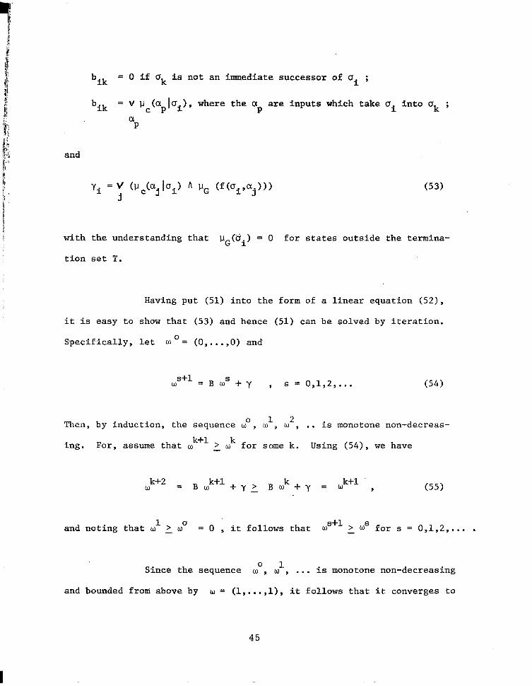
bik = 0 if crk is not an immediate successor of ui ;

bik = V b (a 10 1, where the a are inputs which take ai into uk ; C P i P

a P

and

with the understanding that 1-1 (d. ) = 0 for states outside the termina-

tion set T. G i

Having put (51) into the form of a linear equation (52),

it is easy to show that (53) and hence (51) can be solved by iteration.

Specifically, let w O = (o,.. . ,o> and

w = B w + y , s = 0,1,2,. .. S ( 5 4 )

Then, by induction, the sequence w , w w , .. is monotone non-decreas- ing. For, assume that wk+l wk for some k. Using ( 5 4 ) , we have

0 1 2

and noting that a' 1. w = 0 , it follows that us+' > Us - for s = 0,1,2,. .. . 0

Since the sequence w , w , ... is monotone non-decreasing and bounded froni above by w = (l,...,l), it follows that it converges to

0 1

45

I

the solution of ( 5 2 1 , that is, to the first fi components* of the maximal

goal attainment vector LI,, . Actually, a more detailed argument shows that ( 5 4 ) yields the solution of ( 5 2 ) in not more than fi iterations. In

M

essence, this follows from the fact that if T is reachable from a state

in T’, then it is reachable in R or fewer steps.

To gain an intuitive insight into the above solution, it

is helpful to interpret the transition from ( 4 9 ) to (51) with the aid of

the state diagram of A. Thus, for concreteness assume that A has five

states, with transitions corresponding to various inputs shown in Fig.2.

In this diagram, the number associated with the branch leading from 0

to its successor state via input a is the value of p (a . 1 0 ) . States

a and a are in the termination set and the corresponding values of

p (a. ) are shown alongside. The indicated values of the p ( a . la ) cor-

respond to the constraint sets

i

j C J i

4 6

G 1 C J i

For the system in question, the state transition function

f(o a ) is given by the following table i’ j

46

CLfi Ul “2 (5 3 “4 U5

I CL 1 a4 “3 5 U4 U U 5

cL2 a2 O2 1 U4 ‘(55 (3

From t h i s t a b l e , i t is easy to cons t ruc t the matrix P(IT) f o r any given

policy. For example, for IT = ( a2, al, a2 ), w e have

0 1 0 0

P ( a , a , C L ) = 2 1 2 1: 1 1 0

The system of equations (51) i s obtained by r eve r s ing t he

d i r e c t i o n of f low in each branch (see Fig.3) and t reat ing the s ta tes in

T , t h a t i s , u and u as sources , wi th the states i n T ’ , t h a t i s , U

a2 and u , playing the ro le of receptors ( s inks) . From the diagram

shown in F ig .3 , t he equa t ions i n (51) can be w r i t t e n by inspection. Thus,

4 5 1’

3

47

Employing the simplified notation in which A and v are

replaced by the product and sum, respectively, and wi = pD (ai), i = 1,

2,3, the system of equations (56) becomes

M

u = B w + y (57)

where

B =

0 1 0

0 1 0.8

0.7 0 0

Letting uo = ( o , o , o ) , we o5tain on first interation w1 =

( 0 . 6 , 0 , 0 . 8 ) .

Subsequent iterations yield

u2 = (0.6, 0.8, 0 .8 )

u3 = (0.8, 0.8, 0.8)

u4 = (0.8, 0.8, 0.8)

Thus, u3 = (0.8, 0.8, 0.8) is the solution of (57).

To visualize the iteration process, imagine that each of

the sources in Fig.3 (which are the absorbing states in Fig.2) generates

balls of various diameters, with a i =R+l, ..., n, generating balls i y

48

of diameters ranging from 0 to pG(ai). Furthermore, imagine that a

branch in Fig.2 which leaves state (5 via input a , i s a pipe of diam-

eter p (a I.,) which can carry balls of diameter 2~ (a Iu ) along the

reverse direction, that is, along the direction shown in Fig.3. Thus,

the diagram of Fig.3 may be visualized as a network of pipes whose diam-

i j

c j c j i

eters are indicated in the diagram and which can carry balls of lesser

or equal diameter in the indicated directions. The states in the termi-

nation set (a and 0 1 play the role of sources of balls of diameters up

to p (a ) and p (a ) respectively, while the remaining states (a

and a ) act as receptors. Because the absorbing states act as sources,

we shall refer to the method of solution described above as a reverse-

4 5

G 4 G 5 1’ a2

. 3

flow technique.

Now assume that it takes one unit of time for the balls

to travel from a node of the network of Fig.3 to another node. If we

start with no balls at al, 0 and 0 at time 0, then at time t = 1 2 3 the maximum diameters of balls at a and will be, respec- 1’ 2 3

tively , w w1 and w1 where w = (wl, w2, w ) is the first iter- 1 1 1 1 3 1’ 2 3’

ate of (57). At time t = 2, the maximum diameters of balls will be

given by w2 and at time t = 3 by w . Since it takes no more than 3

three units of time for any ball to travel from its source to any node

in the network, there will be no further increase in the size of balls

at each source upon further iteration. Thus, w gives the maximum

diameter of balls at each receptor node and hence is the desired

solution of (57).

3

49

Turning to the illustration of ( 4 3 ) and the alternation

principle, consider the policy vector 7~ = (al, al, all. For this 7~ , the system of equations ( 4 3 ) becomes

In this case, u1 and a are in T' and 0 is in Ti . Noting that vD (a4 1 IT) = vG (a,) = 1 and 1-1 (a5 I n) = vG (a5) = 0.8,

we find at once vD (01 I .rr) = 0.6 ; pD(u21 IT) = 0.8 ; vD ( 'J31 IT) = 0.8

3 1 2

which is the des ired solution.

Carrying out the same computation for other policy vectors,

we obtain the results tabulated below

(5 1 O2 U 3

0.6 0.8 0.8

0.6 0.6 0.6

0.6 0 0.8

0.6 0 0.6

0.8 0.8 0.8

0 0 0

0 0 0.8

0 0 0

50

1 As a check on the alternation principle, let us take

1 ;

I' IT' = (a,; al, a2) and IT" = (a1, a2, all. Using (47) leads to IT = (a1, a 1,

1,; ! I Note that IT 2 IT' and IT 2 ITTT". From inspection of the table, the maximal

policy is seen to be (a,, al, al). which agrees with the result obtained

by iteration.

The approach to the solution of problems involving implic-

itly defined termination time which we have described in this section can

be extended to more complex decision processes in a fuzzy environment. In

particular, the technique employed for solving the functional equation ( 4 9 )

can readily be extended to fuzzy systems in a fuzzy environment. Furthermore,

( 4 3 ) and ( 4 9 ) can be extended also - as in section 4 - to stochastic finite- state systems. Because of limitations on space, we shall not consider these

cases in the present paper.

7. Concluding Remarks

The task of developing a general theory of decision-

making in a fuzzy environment is one of very considerable magnitude and

complexity. Thus, the results presented in this paper should be viewed

as merely a first attempt at constructing a conceptual framework for

such a theory.

There are many facets of the theory of decision-making

in a fuzzy environment which require more thorough investigation, Among

51

these are the question o f execution of fuzzy decisions; the way in

which the goals and the constraints must be combined when they are of

unequal importance or are interdependent; the control of fuzzy systems

and the implementation of fuzzy algorithms; the notion of fuzzy feed-

back and its effect on decision-making; control of systems in which the

fuzzy environment is partially defined by exemplification; and decision-

making in mixed environments, that is, in environments in which the

imprecision stems from both randomness and fuzziness.

52

1: r

R e f e r e n c e s

1. t. A . Zadeh , "Fuzzy Sets ," I n f o r m a t i o n a n d C o n t r o l , v o l . 8 ,

pp .338-353 , June , 1965.

i: 2. L. A . Zadeh, "Toward a T h e o r y of F u z z y S y s t e m s ,I1 > .

1 1; NASA CR-1432, September 1969 J i

3 . L . A . Z a d e h , " F u z z y I n f o r m a t i o n a n d C o n t r o l ,

vo1.12, p p . 9 9 - 1 0 2 , F e b r u a r y , 1 9 6 8

4. s. 5. L. Chang, I IFuzzy Dynamic Programming and the Decis ion

M a k i n g P r o c e s s , " P r o c . 3 d P r i n c e t o n C o n f e r e n c e o n I n f o r m a t i o n

S c i e n c e s e n d S y s t e m s , p p . 2 0 0 - 2 0 3 , 1969.

5. 5. FU a n d T . J . L i , "On t h e B e h a v i o r o f L e a r n i n g A u t o m a t a

a n d i t s A p p l i c a t i o n s , " T e c h . Rep. TR-EE 68-20, P u r d u e U n i v e r s i t y ,

L a f a y e t t e , I n d i a n a , Aug. 1968.

6. J . Goguen, " L - f u z z y S e t s , " J o u r . Math. Ana l . and App l . , vo l .18 ,

p p . 1 4 5 - 1 7 4 , A p r i l , 1967.

7. J . G . Brown, l t F u z z y S e t s o n B o o l e a n L a t t i c e s , " Rep. No. 1957,

B a l l i s t i c Research L a b o r a t o r i e s , A b e r d e e n , M a r y l a n d , J a n u a r y , 1969.

53

8. A . B e l l m a n , R. K a l a b a a n d L. A . Z a d e h , " A b s t r a c t i o n a n d P a t t e r n

C l a s s i f i c a t i o n , " J o u r . M a t h . A n a l . ' a n d A p p l . , v o 1 . 1 3 , p p . 1 - 7 ,

J a n u a r y , 1966.

9. W . G . Wee, "On G e n e r a l i z a t i o n o f A d a p t i v e A l g o r i t h m s a n d A p p l i c a -

t i o n o f t h e F u z z y S e t C o n c e p t t o P a t t e r n C l a s s i f i c a t i o n , " T e c h n i c a l

R e p o r t TR-EE-67-7, P u r d u e U n i v e r s i t y , L a f a y e t t e , I n d i a n a ; J u l y , 1 9 6 7 .

10. L. A . Z a d e h , " P r o b a b i l i t y M e a s u r e s o f F u z z y E v e n t s , " J o u r . Math.

Ana l . and App l . , vo l .10 , pp .421-427 , Augus t , 1968 .

11. C. L. C h a n g , " F u z z y T o p o l o g i c a l S p a c e s o " J o u r . M a t h . A n a l y s i s a n d

A p p l . , ~ 0 1 . 2 4 , p p . 1 8 2 - 1 9 0 , 1968.

13. J . H. E a t o n a n d L. A. Z a d e h , ' @ O p t i m a l P u r s u i t S t r a t e g i e s i n Discrete-

S t a t e P r o b a b i l i s t i c S y s t e m s , " J o u r . Basic E n g i n e e r i n g (ASME), v o l . 8 4 ,

Ser ies D, pp.23-29 , March , 1962.

14 . J . H . E a t o n a n d L. A. Z a d e h , "An A l t e r n a t i o n P r i n c i p l e f o r O p t i m a l

C o n t r o l , " A u t o m a t i c n a n d R e m o t e C o n t r o l , v o l . 2 4 , p p . 3 2 8 - 3 3 0 , M a r c h , 1 9 6 3 .

15. R . E. B e l l m a n , " D y n a m i c P r o g r a m m i n g , l l P r i n c e t o n U n i v . P r e s s ,

P r i n c e t o n , N.J., 1957.

54

ij 16. V . G. E o l t y a n s k ' i i , R. V. Gamkrelidze, and L. S. P o n t r y a g i n , "On 1'

8' 1 the Theory of Optimal Processas , I l Izv. Akad. Nauk SSSR, vo1.24,

pp.3-42, 1960. I !

19. R. Hellman, " A Markof f i an Dec i s ion P rocess , " Jour. of Math. and r

Mechanics, vo1.6, pp.679-684, 1957.

20. A . A. Howard, "Dynamic Programming and Markoff Processes," M.I.T.

Press and J. Wiley, Inc., Cambridge, Mass. and New York, N . Y . ,

1960.

21. P. Wolfe and G. B. Dantz ig , "Linear Programming in a Markoff

Chain," Oper. Res., vol.10, pp.702-710, 1962.

22. C. Derman and M. K l e i n , "Some Remarks on F in i t e Hor i zon Markof f i an

Decis ion Models , " Opera t ions Research, vo1.13, pp.272-278, 1965. 0

23. C. Derman, "Markof f i an Sequen t i a l Con t ro l P rocesses , - Denumerable

S t a t e S p a c e , " J o u r . Math. Anal. and Appl., vol.10, pp.295-302,

1965.

I. -

24. D. Blackwel l , "Discounted Dynamic Programming, ' l Ann. Math, Stat . ,

~ 0 1 . 3 6 , pp.226-235, 1965.

25. A. F. V e i n o t t , Jr. , "On F i n d i n g O p t i m a l P o l i c i e s i n D i s c r e t e

Dynamic Programming wi th no D iscount ing , ' ' Ann. Math. Stat., vo1.37,

pp.1284-1294, 1966.

2 6 . R. M. Harp and M. He ld , "F in i te -Sta te Processes and Dynamic P ro -

grarnming,ll S I A M J o u r . on Appl. Math., vo1.15, pp.693-718, 1967.

27. E. V . Denardo, "Contract ion Mappings i n the Theory Under l y ing

Dynamic Programming," SIAM Review, vo1.9, pp.165-177, 1967.

56

constraint goal

. . . . . . . . . . .

Fig. 1. Relation between the goal, the constraint and the decision.

57

Q~ 0.6

I

0.8

Fig. 2. State diagram for A.

58

8l c5 0.8 0.8

I

Fig. 3. Reversed-flow s t a t e diagram

NASA-Langley, 1970 - 19 CR-1594

. 59