Decision Makers as Statisticians:

Diversity, Ambiguity and Robustness∗

Nabil I. Al-Najjar†

First draft: October 2006This version: October 2007

Abstract

I study individuals who use frequentist statistical models to drawsecure or robust inferences from i.i.d. data. The main contribution ofthe paper is a steady-state model in which distinct statistical modelsare consistent with empirical evidence, even as data increases withoutbound. Individuals may hold different beliefs and interpret their en-vironment differently even though they know each other’s statisticalmodel and base their inferences on identical data. The behavior mod-eled here is that of rational individuals confronting an environment inwhich learning is hard, rather than ones beset by cognitive limitationsor behavioral biases.

∗ I thank Lance Fortnow, Drew Fudenberg, Ehud Kalai, Peter Klibanoff, Nenad Kos,Charles Manski, Mallesh Pai, and Jonathan Weinstein.† Department of Managerial Economics and Decision Sciences, Kellogg School of Man-

agement, Northwestern University, Evanston IL 60208.e-mail: <al-najjar@northwestern.edu>.Research page : http://www.kellogg.northwestern.edu/faculty/alnajjar/htm/index.htm

Contents

1 Introduction 11.1 Uniform Learning and its Implications . . . . . . . . . . . . . 21.2 Beliefs and Decisions . . . . . . . . . . . . . . . . . . . . . . . 41.3 Robust vs. Bayesian Inference . . . . . . . . . . . . . . . . . . 51.4 Descriptive vs. Normative Interpretations . . . . . . . . . . . 6

2 Uniform Learning and Consistency with Empirical Evidence 72.1 Basic Setup . . . . . . . . . . . . . . . . . . . . . . . . . . . . 72.2 Motivation and Intuition . . . . . . . . . . . . . . . . . . . . . 82.3 Uniform Learning and Statistical Models . . . . . . . . . . . . 112.4 Learning Complexity, Scarcity of Data and the Order of Limits 132.5 Event-Dependent Confidence . . . . . . . . . . . . . . . . . . 15

3 Large Sample Theory 153.1 Exact Learning . . . . . . . . . . . . . . . . . . . . . . . . . . 163.2 Continuous Outcome Spaces . . . . . . . . . . . . . . . . . . . 173.3 Discrete Outcome Spaces . . . . . . . . . . . . . . . . . . . . 183.4 Modeling Choices and Generalizations . . . . . . . . . . . . . 19

4 Diversity, Ambiguity and Decision Making 204.1 A Decision Theoretic Framework . . . . . . . . . . . . . . . . 204.2 Diversity of Beliefs . . . . . . . . . . . . . . . . . . . . . . . . 234.3 Statistical Ambiguity and Probabilistic Closure . . . . . . . . 254.4 Choice over Statistical Models . . . . . . . . . . . . . . . . . . 27

5 Implications and Connections 275.1 Uniform Learning and Vapnik-Chervonenkis Theory . . . . . 275.2 Over-fitting and Falsifiability . . . . . . . . . . . . . . . . . . 295.3 Statistical Models, Coarsening, and Information Partitions . . 305.4 Statistical Models vs. ‘Bounded Rationality’ . . . . . . . . . . 315.5 Bayesian and Frequentist Beliefs . . . . . . . . . . . . . . . . 32

A Proofs 35A.1 Strategic Product Measures . . . . . . . . . . . . . . . . . . . 35A.2 Proof of Theorem 3: Exact Learning . . . . . . . . . . . . . . 35A.3 Proof of Theorem 4: Complete Learning in Continuous Out-

come Spaces . . . . . . . . . . . . . . . . . . . . . . . . . . . . 38A.4 Proof of Theorems 5: Failure of Complete Learning in Dis-

crete Outcome Spaces . . . . . . . . . . . . . . . . . . . . . . 39A.5 Miscellaneous Proofs . . . . . . . . . . . . . . . . . . . . . . . 46

“The crowning intellectualaccomplishment of the brain

is the real world.” 1

1 Introduction

While classical subjectivist decision theory allows for virtually unlimitedfreedom in how beliefs are specified, this freedom is all but extinguishedin economic modeling. Virtually all equilibrium concepts in economics—beit Nash, sequential, or rational expectations equilibrium—require beliefs tocoincide with the true data generating process, reducing any disagreementsin beliefs to differences in information.2 , 3 On the other hand, there is noshortage of examples in the sciences, business or politics where the way in-dividuals ‘look at a problem’ and ‘interpret the evidence’ is just as importantin determining beliefs as the data on which these beliefs are based.

To capture this and other related phenomena, I study individuals facingthe most classical of statistical learning problems, that of drawing inferencesfrom i.i.d. data. These individuals are modeled as classical (frequentist)statisticians concerned with drawing secure or robust inferences. The maincontribution of the paper is to show that distinct statistical models canbe consistent with empirical evidence, even in a steady-state when dataincreases without bound. Individuals may then hold different beliefs andinterpret their environment differently even though they know each other’sstatistical model and base their inferences on identical data.

Decision makers are assumed to be as rational as anyone can reasonablybe. But rationality cannot eliminate the constraints inherent in statisticalinference—any more than it can eliminate other objective constraints likelack of information. The methodology advocated in this paper is to study ra-tional individuals confronting environments in which learning is hard, ratherthan appeal to cognitive limitations or behavioral biases.

1G. Miller: “Trends and debates in cognitive psychology,” Cognition, 1981, vol. 10,pp. 215-25.

2In games with incomplete information, this also requires the common prior assumptionwhich dominates both theoretical and applied literatures.

3The points made in this paragraph are not new. But being part of the folklore ofthe literature, they are hard to trace to original references. The contrast between thesubjectivist and equilibrium methodologies is adapted from Hansen and Sargent (2001).For an exposition of the problems with the Bayesian methodology in statistical inference,see Efron (2005)’s presidential address to the American Statistical Society.

1

1.1 Uniform Learning and its Implications

What makes learning hard? It is intuitive that two individuals with commonexperience driving on US highways will agree on which side of the roadother drivers will use. It is far less obvious that two nutritionists, even whenexposed to a large common pool of data, will necessarily reach the sametheories about the impact of diet on health. These, and countless otherexamples like them, suggest that some learning problems can be vastly moredifficult than others. It is, however, not at all clear what this formally means:learning the probability of any single event in an i.i.d. setting reduces to thesimple problem of learning from a sequence of coin flips. This is so regardlessof how ‘complicated’ the event, the true distribution, or the outcome spaceis.

Focusing on learning probabilities ‘one event at a time,’ misses the point,however. Decision making is, by definition, about choosing from a family offeasible acts. From a learning perspective, this raises the radically differentand more difficult problem of using one sample to learn the probabilities ofa family of events simultaneously.

The theory of uniform learning is the formal framework that studies ro-bust (i.e., distribution-free) inference in this context.4 In Section 2, I usethis theory to introduce a simple model of belief formation where probabil-ities are estimated from empirical frequencies using a frequentist statisticalmodel. Any such model gives rise to a belief correspondence that maps obser-vations to a set of probability measures consistent with empirical evidence.

The individual chooses confidence levels in his estimates of various events.This choice is trivial when data is abundant and the set of alternatives tochoose from is narrowly defined. An example is repeated i.i.d. coin flipsor, more generally, a finite outcome space and data that asymptotically in-creases without bound. In this case, frequentist, Bayesian, and just aboutany other sensible inference all agree.

The more interesting case is situations characterized by scarcity of data.A key insight from the theory of uniform learning concerns the tension be-tween the amount of data, and the ‘richness’ of the structure of acts thedecision maker wants to evaluate. What makes a learning problem hard isnot the amount of data per se, but this amount in relation to the ‘statisti-

4This theory, also known as Vapnik-Chervonenkis theory, and its generalization, thetheory of empirical processes, occupy a central role in modern statistics but are relativelyunknown to economic theorists. The reason for this is clear and revealing: a Bayesian hasno use for uniform learning.

2

cal complexity’ of the alternatives considered. Thus, the impact-of-diet-on-health problem is hard because one is concerned with learning about manyevents simultaneously, namely how different diets impact individuals withdifferent characteristics. The theory of uniform learning provides a formalframework to make sense of intuitive notions like a set of events is ‘rich,’‘hard to learn’ or ‘statistically complex.’

With abundant data and a narrowly defined decision problem beliefsare (approximately) determinate: the set of measures consistent with em-pirical evidence collapses to a small (ε-) neighborhood and little scope fordisagreement remains. But when data is scarce and the decision maker hasto evaluate a rich set of options, the result is statistical ambiguity, in thesense that data is insufficient to pin down beliefs. In this case, differentindividuals with different statistical models may draw different inferencesand hold wildly different beliefs even though they observe the same dataand know each others’ models.

An implication of this theory is a sort of ‘law of conservation of confi-dence:’ as the individual increases confidence in his estimates of the proba-bility of some events, he inevitably decreases his confidence in others.5 Thistrade-off has interesting implications for confidence-sensitive decision mak-ers. First, as discussed earlier, beliefs may be under-determined by empiricalevidence. Second, although ambiguity about the probability of some eventsdisappears as the number of observations increases, ambiguity about oth-ers persists. On the statistically unambiguous events, the decision makerhas Bayesian beliefs6 but this is now a consequence of the learning modelrather than an aspect of preferences. Third, coarsening and categorizationare necessary for learning. The pervasiveness of categorization seems beyonddispute and does not require a model to establish. Why people categorizeis less obvious and is potentially the more important question: do individu-als categorize because of computational complexity, limited memory, lack ofinformation? If decision makers are modeled as classical, frequentist statis-ticians, then categorization is necessary to draw secure inferences. Since themodel is free of any presumed a priori structure, any implied categorizationreflects individuals’ attempt to make sense of their environment (hence theopening quote of this paper). No appeal to computational complexity or

5The reader may find it helpful to compare this with ordinary linear regression, whereadding more regressors lowers the confidence in the estimated parameters. A key differ-ence here is that our setting is non-parametric. The need for a non-parametric model isdiscussed at length in Section 3.4.

6That is, a single (additive) probability measure that is updated using Bayes rule.

3

cognitive limitations is made.In Section 3, I turn to large sample theory, where the main technical con-

tribution of this paper lies. The known theory of uniform learning primarilyfocuses on the case of finite data and has no bite in the limit, as the amountof data increases. This makes it unsuitable for use in most economic models.On a practical level, large sample theories permit greater tractability andclearer intuitions. More fundamentally, equilibrium notions in economics—e.g., Nash or rational expectations equilibrium—are usually interpreted ascapturing insights about steady-state or long-run behavior. A theory oflearning in which diversity is nothing more than a temporary phenomenonwould be difficult to reconcile with this steady-state interpretation.7

1.2 Beliefs and Decisions

The main concern of this paper is with belief formation, with questionslike: where do beliefs come from? and what makes them ‘reasonable?’ Anorthogonal, but equally important, question is: what decisions do individualsmake given their beliefs? To answer this, a decision making model thatcombines beliefs and tastes into choices is needed. In Section 4, I introducea simple framework to integrate uniform learning into standard models ofdecision making and their applications.

One issue I address using this framework is whether learning consider-ations lead rational decision makers to hold common beliefs. See Morris(1995) for a survey and synthesis. One of the clearest statements of one sideof the argument is Aumann (1987, pp. 12-13):

“[T]he CPA expresses the view that probabilities should be based oninformation; that people with different information may legitimatelyentertain different probabilities, but there is no rational basis for peoplewho have always been fed precisely the same information to do so.”

At the other end of the argument, Savage (1954) writes:8

“[I]t is appealing to suppose that, if two individuals in the same situa-tion, having the same tastes and supplied with the same information,act reasonably, they will act in the same way. [....] Personally, I

7This point, often under-appreciated, is discussed at length in Bewley (1988) whointroduced the notion “undicoverability” to capture the idea of stochastic processes thatcannot be learned from data. His model and analysis are, however, quite different fromwhat is reported here.

8Page numbers refer to the 1972 edition, Savage (1972).

4

believe that [such agreement] does not correspond even roughly withreality, but, having at the moment no strong argument behind my pes-simism on this point, I do not insist on it. But I do insist that, untilthe contrary be demonstrated, we must be prepared to find reasoninginadequate to bring about complete agreement. [...] It may be, andindeed I believe, that there is an element in decision apart from taste,about which, like taste itself, there is no disputing.” (p. 7)

In reconciling these conflicting views, it is a good idea to have in mind anexplicit model that explains how “probabilities should be based on informa-tion.” My claim is that, when viewed as statisticians, it is perfectly naturalfor individuals to hold different beliefs based on identical information. Theirstatistical models may be interpreted as Savage’s “element in decision apartfrom taste, about which [...] there is no disputing.”

1.3 Robust vs. Bayesian Inference

The reader imbued with the Bayesian paradigm may be bewildered by no-tions of learning and robustness that make no reference to prior beliefs,updating rules and the like. Besides, doesn’t the standard Bayesian modelalready contain a theory of belief formation in the form of updating viaBayes rule?

Separating belief formation from decision making, as done in this paper,may seem like a serious violation of the Bayesian paradigm. Historically,however, Savage conceived his framework as normative, as a way to definerational behavior in situations involving uncertainty, but that is otherwisesilent on the question of belief formation. Thus, he writes (1967, p. 307)that the subjectivist view of probability is best thought of as a tool “bywhich a person can police his own potential decisions for incoherency.” Thisdoes not seem to commit even a Bayesian to any particular model of beliefformation.

A common retort is that Bayesian theory already provides a theory ofbelief formation via de Finetti’s theorem. The need for a separate model ofbelief formation is obviated, so the argument goes, by assuming a decisionmaker with exchangeable beliefs who updates his prior using Bayes rule. Theeffectiveness of this as a ‘learning’ and ‘belief formation’ procedure is deeplyentrenched in the Bayesian folklore, but it is also a myth. A classic theoremby Freedman (1965), detailed in Section 5.5, shows that Bayesian posteriorsare “generically” erratic in a very strong sense whenever the outcome space

5

is infinite.9 Although there is always room to quibble over the meaningof genericity of beliefs and probability laws, what seems beyond dispute isthe impossibility of a general result establishing the consistency of Bayesianupdating. In a survey of that literature, Diaconis and Freedman (1986, p.14) write:

“Unfortunately, in high-dimensional problems, arbitrary details of theprior can really matter; indeed, the prior can swamp the data, no mat-ter how much data you have.”

Our intuition, often naively derived from coins and urns, that data eventu-ally swamps the priors is misleading. Freedman (1965) puts it quite vividly:

“[F]or essentially any pair of Bayesians, each thinks the other is crazy.”

If one substantially relaxes Bayesian theory, then there is not even a consen-sus on how to update beliefs to incorporate new evidence.10 In summary, theerratic nature of Bayesian decision making and its inability to incorporaterobustness suggest that one should not be quick to dismiss non-Bayesianinference as irrational.

1.4 Descriptive vs. Normative Interpretations

Readers who declare frequentist statisticians irrational will have a hard timenot just with this paper, but with current statistical practice in all empiri-cal fields of enquiry–which is overwhelmingly frequentist.11 At a minimum,frequentist decision making is worth studying because it is descriptively im-portant, and may therefore be a better approximation of how economicactors behave.

There are also reasons to think that a concern for robustness is norma-tively compelling. In his 1951 paper, Savage states that “the central problemof statistics is [..] to make reasonably secure statements on the basis of in-complete information.” What applies to statisticians ought to apply just aswell to economic actors. The fact that the classic Savage (1954) frameworkprecludes concerns for security led to many subsequent attempts to rein-troduce such concerns. These include Bewley’s ((1986) and (1988)) studies

9Freedman’s result holds when the outcome space is the set of integers. It was gener-alized by Feldman (1991) to complete separable outcome spaces, such as [0, 1] or Rn.

10Such as preferences not supported by a single prior, as in ambiguity models, forinstance. See Machina (1989)’s classic survey of these issues, especially the resultingproblem of dynamic (in-)consistency.

11 See, for instance, Efron ((2005) and (1986)).

6

of Knightian uncertainty, the ambiguity models of Schmeidler (1989) andGilboa and Schmeidler (1989), the macroeconomics literature on robustnessand model uncertainty pioneered by Hansen and Sargent (e.g., see their 2001expository paper), and the econometrics literature that uses minimax regretor other robustness criteria as found, for instance, in Manski (2004).

Although classical frequentist methods dominate empirical studies ineconomics, they had negligible impact on economic theorizing. One areawhere frequentist-like procedures appear is the literature on learning ingames, as in models of fictitious play, adaptive learning and regret matching.Another example is Kreps (1998)’s model of anticipated utility, aspects ofwhich he attributes to the older literature on learning rational expectations.

Hansen and Sargent (2001, p. 215) argue that a fundamental aspect ofthe economic methodology is what might be termed inferential symmetry,namely that “the economist and the agents inside his model [be] on thesame footing” and, in particular, that “economic agents share the modelers’doubts” and concerns for robustness. In light of this, it is puzzling that wechoose frequentist methods to learn about the behavior of economic agentsand their environments, yet assume that these very agents are Bayesianswhen learning about the same environment.

2 Uniform Learning and Consistency with Empir-ical Evidence

2.1 Basic Setup

A decision maker faces a set of outcomes X with a σ-algebra of events Σ anda true but unknown probability distribution P in P, the set of probabilitymeasures on (X,Σ). Here we focus exclusively on statistical inference andbelief formation; decision making is examined in Section 4.

I consider three models, with the third not used until Section 3.3:

1. Xf is a finite set, Σ = 2Xf is the set of all subsets, and P is the set ofall probability measures;

2. Xc is a complete separable metric space, Σ = B is the family of Borelsets, and P is the set of countably additive probability measures;

3. Xd is a countable set, Σ = 2Xd is the set of all subsets, and P is theset of finitely additive probabilities.

7

To simplify the notation, we will distinguish the probability spaces (asXf , Xc or Xd) but not the sets of events Σ or probabilities P as they willalways be clear from the context. Definitions, claims and interpretationsrelating to an outcome space X are meant to apply to all three possibilitieslisted above.

The decision maker bases his beliefs on repeated i.i.d. sampling fromthe fixed true distribution P on X. Finite samples of t observations aremodeled by conditioning on the first t coordinates of an infinite samples = (x1, . . .). Formally, let S denote the set of all infinite sequences ofelements in X, interpreted as outcomes of infinite sampling. I.i.d. samplingunder P corresponds to the product probability measure P∞ on (S,S), whereS is the σ-algebra generated by the product topology.12

2.2 Motivation and Intuition

This subsection focuses on the special class of categorization problems tointroduce and motivate the main ideas.

Definition 1 A decision maker faces a categorization problem if:

• X is of the form Y × a, b for some set of “instances” Y and twocategories, a and b;

• The decision maker chooses an element of F , the set of all functionsf : Y → a, b, interpreted as categorization rules;

• Given P , his payoff from f is P(y, i) : f(y) = i, i = a, b.

As an example, consider a stylized investment problem where an investorfaces randomly drawn “investment opportunities” from a set Y . A catego-rization rule is a contingent investment strategy f : Y → buy, sell. Givensuch f , a correct categorization is made at x = (y, i) if f(y) = i. His payoffis simply the probability of the set of outcomes where he ‘gets it right:’

Af ≡ (y, i) ∈ X : f(y) = i.

To convert this problem into a standard decision theoretic language, a nat-ural state space is P and acts are functions from P to monetary payoffs in

12Most readers are familiar with these standard concepts in the cases Xf and Xc. SectionA.1 provides the requisite background in general enough terms to cover the less familiarcase of (Xd,Σ).

8

[0, 1].13 We restrict attention to categorization acts:

ξ : P → [0, 1]

such that for every P , ξ(P ) = P (Af ) for some f ∈ F . For a Bayesiandecision maker, this is a completely straightforward problem. He wouldhave a belief π over P and chooses the investment rule that maximizesexpected payoff given his belief.

We are interested in the case where no such belief is given as a primitive,but must rather be constructed from experience. Specifically, the decisionmaker observes a sequence st = (x1, . . . , xt) drawn i.i.d. from P . In ourinvestment example, the stationarity of P may be interpreted as consistingof two parts: (a) the description of each investment opportunity is com-prehensive enough that no potentially relevant factors are omitted; and (b)the economic fundamentals of what makes a company or a stock profitableare stable. If the underlying distribution is non-stationary, then one wouldexpect learning to be even harder, and for reasons quite distinct from thosewe wish to emphasize here.

I will take the point of view that the decision maker is a frequentistwho is concerned with obtaining secure inferences. Difficulties with theBayesian procedure of starting with a prior and update it using the datawere discussed in the Introduction and will be further elaborated in Section5.5.

Define the empirical frequency of A ⊂ X relative to a sample st:

νt(A, s) ≡ #(x1, . . . , xt) ∩At

.14 (1)

An application of your favorite version of the weak law of large numbersensures that νt(Af , s) is a good estimate of ξ(P ) ≡ P (Af ) when t is large.For example, by Chebyshev’s inequality one has, for any f ∈ F :

P∞s : |P (Af )− νt(Af , s)| < ε > 1− 14tε2

.

13Assume risk neutrality throughout this example for simplicity.14In the special structure of categorization problems, the data is in the form of a sequence

st = (yr, ir)tr=1 of t instance-category pairs and the empirical frequency of Af is

νt(Af , st) =

#f(yr) = irt

.

9

In fact, probabilities can be estimated uniformly regardless of the event orthe distribution:

supf∈F

supP∈P

P∞s : |P (Af )− νt(A, s)| < ε > 1− 14tε2

. (2)

It is irrelevant whether f is complicated or simple, the outcome space X isfinite or infinite, . . . etc. The inference about any single rule boils down toestimating the probability of one event, and this is formally equivalent tofinding the probability of heads in independent coin flips. This may be oneof the reasons behind the commonly held intuition that “people eventuallylearn.”

But choice involves, almost by definition, evaluating many acts simulta-neously. In the investment example, one has to evaluate the performance ofas many candidate investment rules as possible in order to choose the bestone. Taking a learning perspective, define the set of ε-good samples for f as:

Good tε,P (f) ≡s :∣∣P (Af )− νt(Af , s)

∣∣ < ε

This is the set of samples on which the empirical frequency of Af is a goodestimate of its true probability. Here the parameter ε may be viewed as ameasure of the confidence one has in this approximation.

Suppose now we are choosing among rules f1, . . . , fI and there isenough data to ensure that each event Good tε,P (Afi) has high probability.Then, by definition, we can confidently assess the performance of any givenrule fi. This, however, says little about how to confidently choose the bestrule within the set f1, . . . , fI since this requires samples that are represen-tative for each event Af1 , . . . , AfI simultaneously. That is, one has to ensurethat the probability:

P∞[∩iGood tε,P (Afi)

]. (3)

is large. The fact that each event Good tε,P (Afi) is large guarantees only thatthe probability of the intersection is at least 1−Iε, a conclusion that quicklybecomes useless as the number of rules being compared increases.

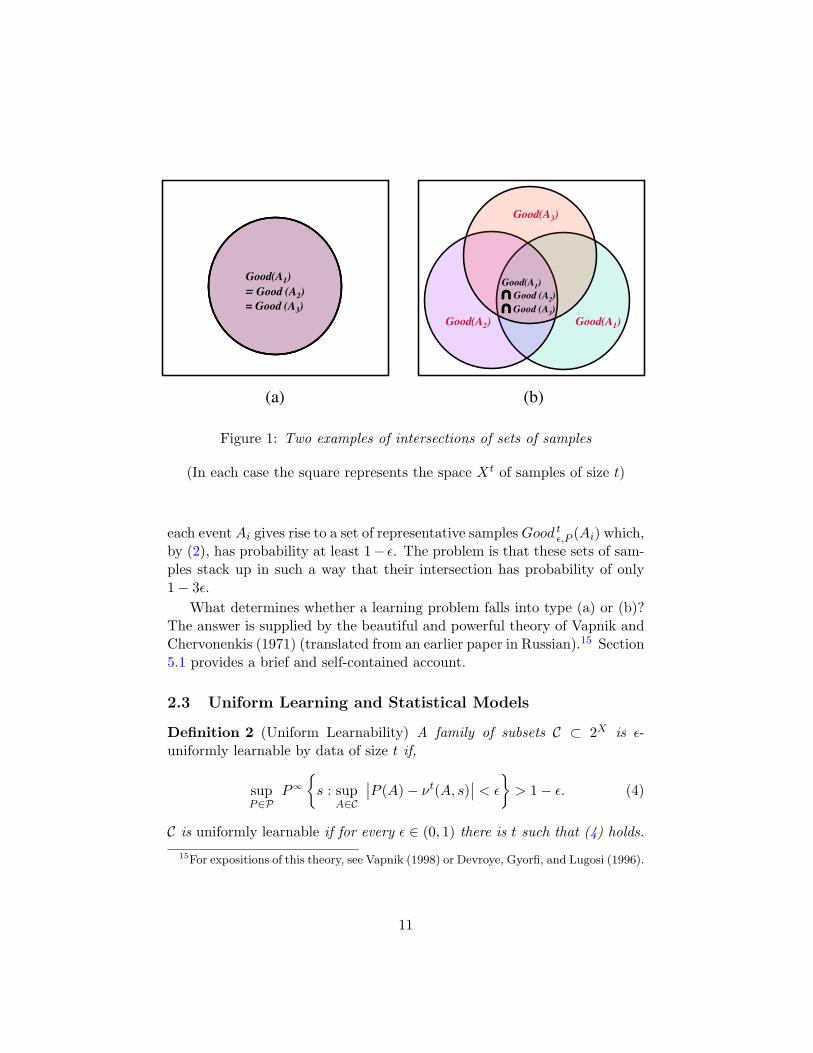
The central issue is to determine for what class of events is uniformlearning possible. This is illustrated in Figure 1 where the square repre-sents the set of all samples of length t and the comparison is among threeevents A1, A2, and A3 in the outcome space X. In Figure 1(a) the eventsGood tε,P (Ai), i = 1, 2, 3, coincide so their intersection has probability 1− ε.In this case, one has as much confidence in the joint evaluation of the threeevents as in each event simultaneously. Part (b) illustrates opposite case:

10

The square represents the space Xt of samples of size t

For an event A, GoodA is the set of

representative samples relative to the event A

Good(A1)Good(A2)

Good(A3)

Good(A1)

= Good (A2)

= Good (A3)

(a)

Good(A1)

! Good (A2)

! Good (A3)

(b)

Figure 1: Two examples of intersections of sets of samples

(In each case the square represents the space Xt of samples of size t)

each event Ai gives rise to a set of representative samples Good tε,P (Ai) which,by (2), has probability at least 1− ε. The problem is that these sets of sam-ples stack up in such a way that their intersection has probability of only1− 3ε.

What determines whether a learning problem falls into type (a) or (b)?The answer is supplied by the beautiful and powerful theory of Vapnik andChervonenkis (1971) (translated from an earlier paper in Russian).15 Section5.1 provides a brief and self-contained account.

2.3 Uniform Learning and Statistical Models

Definition 2 (Uniform Learnability) A family of subsets C ⊂ 2X is ε-uniformly learnable by data of size t if,

supP∈P

P∞s : sup

A∈C

∣∣P (A)− νt(A, s)∣∣ < ε

> 1− ε. (4)

C is uniformly learnable if for every ε ∈ (0, 1) there is t such that (4) holds.15For expositions of this theory, see Vapnik (1998) or Devroye, Gyorfi, and Lugosi (1996).

11

The crucial aspect of the definition is the location of supA∈C , indicating therequirement that the probability being evaluated in (4) is that of samplesin which all events in C have their probabilities ε-close to their empiricalfrequencies.

Definition 3 (Statistical Models) A triple (C, ε, t) is a (feasible) statisticalmodel whenever C is ε-uniformly learnable with data of size t.

For each event A, think of νt(A, s) as a “point-estimate” of P (A) and ε asdenoting the boundaries of a confidence interval around νt(A, s). Extendingthis idea to all events, define

µtC,ε(s) =p ∈ P : sup

A∈C

∣∣p(A)− νt(A, s)∣∣ ≤ ε . (5)

as the set of distributions consistent with empirical evidence. A probabilitymeasure that does not belong to µtC,ε is one that can be rejected with highconfidence as inconsistent with the data. We suppress reference to C and ε,simply writing µt(s), whenever they are clear from the context.

We shall view the collection of events C and the degree of confidence εas reflecting the decision maker’s model of his environment. On the otherhand, the amount of data t is an objective constraint that confronts thedecision maker with a trade-off between confidence, measured by ε, and thescope of events C he can learn.

The problem with this logic is that feasibility of a statistical model, byitself, is a hopelessly weak criterion; it is, for instance, trivially satisfied whenC = ∅ or ε = 1.16 To obtain a meaningful theory, it is useful to introducethe following partial order on statistical models:

Definition 4 A statistical model (C′, ε′, t′) dominates another model (C, ε, t)if

• C ⊆ C′, ε′ ≥ ε and t′ ≤ t.

(C′, ε′, t′) strictly dominates (C, ε, t) if at least one of the above inequalitiesholds strictly.

When considering decision makers’ preferences over statistical models inSection 4.4, I will argue that it is normatively compelling that scarce datais not wasted. Thus, the most relevant statistical models must be maximal:

16In typical statistical learning theory applications, the family of events C is exogenouslygiven, such as half intervals in [0,1], or rectangles in R2. I know of no instance in whichthe idea of maximality is used in that literature.

12

Definition 5 (Maximality) A statistical model (C, ε, t) is maximal if thereis no feasible model (C′, ε′, t′) that strictly dominates it.

A maximal model does not overlook any sharper inferences that could havebeen drawn using the same amount of data t.

For a finite outcome space Xf , the existence of a maximal model thatdominates a given model (C, ε, t) is straightforward. This is more delicateon infinite outcome spaces, but still true:

Theorem 1 Fix t and suppose that (C, ε, t) is a feasible statistical model.Then there is a maximal feasible statistical model (C′, ε′, t′) that dominates(C, ε, t).

2.4 Learning Complexity, Scarcity of Data and the Order ofLimits

A key theme of this paper is that the desire to draw secure inferences fromscarce data leads individuals to statistical models that are coarser than thetrue model. This is captured by the criterion of uniform learnability, whichreflects the difficulty of learning when data is scarce relative to the set ofoptions available to the decision maker. Recall that the weak law of largenumbers implies that there is t such that for all t > t

supA∈C

supP∈P

P∞s :∣∣P (A)− νt(A, s)

∣∣ < ε> 1− ε. (6)

This bound pertains to a statistical experiment in which a fresh sampleis drawn for each event evaluated. Each new event would require t newobservations, a preposterous amount of data when the decision maker iscomparing a large set of acts.

A concern for scarcity of data means that data is not so abundant thatone can generate samples at will. The uniform learning criterion

supP∈P

P∞s : sup

A∈C

∣∣P (A)− νt(A, s)∣∣ < ε

> 1− ε (7)

models a decision maker who gets one shot at sampling t observations. Thescarcity of data forces the decision maker to restrict attention to a narrowerclass of events C.

In summary, modeling environments where learning is hard is an illusivegoal because no event, when taken in isolation, is ever hard to learn. Rather,

13

complexity in learning is a property of families of events and arises only whenthe scarcity of data is taken seriously.

Whether a decision problem is complex or not depends on the relation-ship between the amount of data available and the richness of the set ofevents considered. This is sharply illustrated in the following theorem:

Theorem 2 Let X = Xf be a finite outcome space with cardinality n. Then:

1. For any given n and ε > 0 there is t such that 2Xf is uniformly learn-able with data of size t ≥ t; and

2. Given any t, ε > 0 and α > 0 there is n such that #Xf > n implies:

#C#2Xf

< α

for any C that is ε-uniformly learnable with data of size t.

The problem is one of order of limits: Holding the finite set of outcomesfixed, taking the amount of data to infinity guarantees uniform learning ofthe powerset. On the other hand, holding t large but fixed, the set of eventsand acts that can be uniformly learned shrinks down to zero as the size of theoutcome space increases. This is even when t is large enough to guaranteelearning the probability of any event in isolation.

If the outcome space is ‘small,’ as in the case of coin flips, the side of theroad drivers are likely to use and so on, then case 1 of the theorem is rele-vant. Things differ dramatically when the outcome space is vast. Consider,for example, the problem of evaluating the impact of diet on health. If thereare z1 binary attributes that define an individual’s characteristics, z2 binaryattributes that define diet characteristics, and z3 binary attributes that de-fine health consequences, then the cardinality of the finite outcome space is2z1+z2+z3 . For entirely conservative values of, say, z1 + z2 + z3 = 50, thecardinality of the set of events is the incomprehensibly large number 2250

.For individuals to reach agreement on the probability of all events throughlearning is more in the realm of fantasy, even by the standard of idealizedeconomic models of decision making.17

When part 2 of the theorem is relevant, as in the last example, individualsseeking robust inferences from a large but limited pool of data either restrict

17The reader may be amused by the fact that complete 0.01-agreement will require,using (17), a minimum t that exceeds the estimated number of minutes since the BigBang.

14

the scope of theories C, the set of models they consider P, or both. The keypoint is that such restrictions must precede empirical evidence. It shouldtherefore not be surprising that rational individuals entertain ambiguity anddisagreements even when facing identical information.

2.5 Event-Dependent Confidence

The model presented above is unnecessarily restrictive in that it rules outtrading off confidence across events. Consider, for example, a choice betweena bet that pays 1 on an event A and zero otherwise, and another that pays100 on B and -50 otherwise. One would expect a decision maker to demandgreater precision about his estimate of P (B) than P (A).

The formalism used so far assumes a common confidence interval size εfor all events. This is done for simplicity, and a generalization can be readilymade. Instead of a single ε applied to a family of events C, confidence isnow represented by

• A function ζ : Σ → [0, 1], representing an event-dependent (size of)confidence interval;

• A constant δ ∈ [0, 1] representing a confidence level.

Uniformly learnable would then mean:

supP∈P

P∞s : ∀A,

∣∣P (A)− νt(A, s)∣∣ < ζ(A)

> δ. (8)

Our more restrictive formulation (C, ε, t) is one characterized by δ = ε anda distinguished family of events C such that ζ(A) = ε for each A ∈ C. Thearguments of the paper go through, with appropriate modifications, underthe more general model.

3 Large Sample Theory

I now turn to the asymptotic properties of uniform learning as the amountof data increases. There are at least three reasons why large outcome spacesare important:

• Robustness: A natural question is: would the conclusions of the anal-ysis eventually disappear as more data accumulates?

15

• Tractability: Asymptotic models can be considerably simpler and yieldsharper intuitions.

• Applicability: Equilibria in economic and game theoretic models areoften viewed as steady-states that arise as limits of learning processes.

3.1 Exact Learning

As the decision maker is given more data, he can sharpen his statisticalmodel by either decreasing ε or increasing the range of events C he learnsabout. We formalize this using the notion of learning strategy:

Definition 6 A learning strategy is a sequence σ ≡ (Ct, εt, t)∞t=1 of sta-tistical models satisfying:

• εt → 0;

• Ct ⊆ Ct+1 for every t;

• Ct is a maximal εt-uniformly learnable family of events by data of sizet.

The learning strategy is simple if there is t such that Ct = Ct+1 for everyt ≥ t.

The idea is that, as the decision maker is given larger sets of data, the set offeasible statistical models increases. His choice from the larger set of modelsmay either involve increasing confidence or enlarging C. Simple strategiesinvolve increasing confidence while holding the set of events C constant.

Given a learning strategy σ = (Ct, εt, t)∞t=1, the set of beliefs consistentwith empirical evidence is:

µσ(s) ≡p : ∀t sup

A∈Ct

∣∣p(A)− νt(A, s)∣∣ ≤ εt .

The next theorem shows that on a ‘typical’ sample, any p ∈ µσ(s) shouldassign to any event A a probability equal to the true probability P (A), andthus µσ(s) has a very clean structure on most samples:

Theorem 3 (Exact Learning) Fix any learning strategy (Ct, εt, t) andwrite C = ∪tCt. Then for any P ∈ P:

µσ(s) =p : p(A) = P (A), ∀A ∈ C

, P∞ − a.s.

In particular, µσ(s) is a convex set of probability measures, almost surely.

16

The main challenge in proving this result is to show that it holds for finitelyadditive P on Xd, as required in Section 3.3 below. Note also that agreementon C may lead to agreement on events outside C. See Section 4.3.

The theorem justifies the following straightforward definition:

Definition 7 Beliefs are asymptotically determinate if there is a learningstrategy σ such that for every P ,

µσ(s) = P, P∞ − a.s.

That is, the only belief consistent with empirical evidence is the true distri-bution.

The phenomenon of most interest to us is beliefs that are not determi-nate. An easy consequence of Theorem 2 is that this cannot be achieved ifX is finite. To model environments where learning is hard, data is scarce,and beliefs are indeterminate, we need to turn to infinite outcome spaces.

3.2 Continuous Outcome Spaces

An obvious candidate for an infinite outcome space is Xc, a complete sepa-rable metric space with the Borel σ-algebra B. P is the set of all (countablyadditive) probability measures on (Xc,B). We begin with a general, anddiscouraging, result:

Theorem 4 If X is a complete metric space then beliefs are asymptoticallydeterminate via a simple learning strategy.

A prototypical example illustrating the theorem is:

Example 1 Let X = [0, 1] and C be the class of half intervals: [0, r] or (r, 1]where r is any number in [0, 1]. Then this is an uncountable collection ofevents that is uniformly learnable.

There are two distinct learning principles at play in this example:

• Statistical learning: by the classic Glivenko-Cantelli Theorem, the em-pirical distribution functions converge to the distribution function uni-formly almost surely, so in the limit the probability of each half intervalis known without error;

• Deduction: once the probabilities of events in C are known one can usethe axioms of probability to deduce the probabilities of events outsideC. In this example, this leads to deducing the probabilities of all Borelevents. The theorem shows that this intuition generalizes.

17

The argument underlying the theorem shows that complete learning inthe limit can be achieved using an exceedingly simple class of events, similarin their simplicity to the half intervals. It is difficult to think of boundedrationality reasons that would prevent a decision maker from using suchsimple learning procedure.

The example is disturbing in another way, namely that it reveals a rathersharp disconnect with the finite outcome space/finite data model. It is easyto find examples of finite outcome space and finite data in which completelearning does not occur. Yet this cannot occur in the settings covered inTheorem 4. This is an artifact of the mathematical structure of Xc thatdistorts the learning problem by imposing strong restrictions on Σ and P.This leads to the model of the next section in which complete learningcannot occur, reflecting more faithfully the phenomenon found in finite-finite models.

3.3 Discrete Outcome Spaces

Here we consider Xd to be countable; Σ is the set of all subsets of X; andP the set of all finitely additive probability measures on Σ. This spaceof outcomes is discrete in the sense that there is no extraneous metric ormeasurable structure that restricts the set of events.

Theorem 5 Beliefs in the discrete outcome space (Xd,Σ) are not asymp-totically determinate.

In fact, for any learning strategy σ, there is P such that µσ(s) 6= P,P -a.s.18

It is worth noting that the scope of disagreement asserted in the theoremcan be substantial, as shown in the following corollary to its proof:

Corollary 6 For any uniformly learnable C and any α ∈ (0, 0.5] there is apair of probability measures λ and γ that agree on C, yet |λ(B)− γ(B)| = α

for uncountably many events B.

To interpret these results, recall the earlier discussion that there aretwo learning principles: a statistical principle, under which probabilities arededuced from data, and a deductive principle, under which probabilitiesof some events are deduced from knowledge of the probabilities of others.

18This is a stronger claim than just saying that beliefs are not asymptotically determi-nate, which would have only required that µσ(s) 6= P on some set A with P (A) > 0.

18

Statistical inference works here just like it did in continuous outcome spaces.What is different is that there is no longer a uniformly learnable C suchthat the probability of all events can be deduced from knowledge of theprobability of events in C.

The proof uses a combinatorial result that bounds the “size” of uniformlylearnable classes of events. Passing to the limit is quite delicate because,among other things, the cardinality of a family of events is not a usefulmeasure of its learning complexity.19 The proof uses a novel argument inwhich a (finitely additive) measure λ can be perturbed without changingthe probability it assigns to events in C.

3.4 Modeling Choices and Generalizations

3.4.1 The Absence of Presumed Structure

A finite outcome space Xf is free from any presumed a priori structure, suchas notions of distance, ordering, or similarity between elements. I view astructure-free model as an essential backdrop to any study that seeks toshed light on how individuals model their environment. No one disputesthat cognitive structures, like orderings and similarity, are essential in de-cision making. But to explain why these structures look the way they do,one should avoid letting extraneous presumed structures surreptitiously con-taminate the analysis. In a structure-free model, like Xf , individuals end upusing orderings and similarity in the form of a statistical model to facilitatelearning and to make sense of empirical evidence (hence the opening quoteof this paper).

In infinite outcome spaces, the counterpart of Xf is the discrete spaceXd, which admits all subsets and all probability measures as legitimate. Bycontrast, the continuous outcome space Xc comes loaded with structural as-sumptions. When Xc = [0, 1], for instance, a similarity function in the formof a metric is implied, limiting the range of events, acts, and probabilitiesused. This accounts for the learning result, Theorem 4, that stands in starkcontrast to what happens in large but finite outcome spaces.

3.4.2 Stationarity

The model assumes that the decision maker faces a stationary problem (Pis unchanging). Many decision problems may be usefully modeled as sta-

19The example in footnote 25 illustrates that knowledge of the probabilities of a count-able family may be sufficient to determine the probabilities of all Borel sets.

19

tionary, while some non-stationary problems become stationary in a richeroutcome space. In any event, failure of learning would hold a fortiori in non-stationary settings where the object to be learned is constantly changing.

3.4.3 Robustness

Robustness enters via our assumption that the decision maker is completelyignorant about the true model P , and that he seeks inferences robust to thismodel uncertainty. This may be viewed as too extreme. In defense of thisrequirement, consider:

• The model can accommodate the introduction of prior knowledge thatnarrows down the set of possible distributions. The qualitative insightsgeneralize if we limit the decision maker’s model uncertainly to someP ( P, provided this is a rich enough set of distributions.

• But one must then ask where does knowledge of P come from? Therequirement to be robust to all distributions helps delineate the bound-ary between empirically-grounded and extra-factual sources of knowl-edge.

In the investment example, allowing all P ’s may correspond to a technicalinvestor with no prior theory (e.g., basic economics or finance) that puts apriori restrictions on the true distribution. If the investor were to incorporatetheories from macroeconomics or finance, say, he will presumably be ableto reduce P to some smaller set P. But despite decades of extensive andcommonly shared evidence, even the best theories these fields have to offerleave ample room for model uncertainty. This is seen daily in well-publicizedconflicting policy recommendations, forecasts, and investment strategies.

4 Diversity, Ambiguity and Decision Making

4.1 A Decision Theoretic Framework

Learning leads to a compact convex set of probability measures µt(s) andµσ(s) consistent with empirical evidence. These are purely statistical con-structs that impose constraints on beliefs, but otherwise orthogonal to howbeliefs are incorporated into choice. To do so requires an explicit decisiontheoretic framework.

20

Here I use a simple formulation based on Gajdos, Hayashi, Tallon, andVergnaud (2006)’s model of how objective information can be incorporatedinto a subjective setting. Fix a finite set of consequences Z. An act is afunction of the form:

ξ : P → ∆(Z).

Here, P is interpreted as the set of states and ∆(P) as an individual’s beliefsabout these states. For example, ξ may be induced by a categorization rule,as detailed in Section 2.2. Endow P and ∆(P) with their weak* topologies,20

and let K be the set of all compact and convex subsets of ∆(P).Consider now a decision maker with objective information that the true

distribution π over the states space P lies in some compact convex set Π ⊆∆(P). Gajdos, Hayashi, Tallon, and Vergnaud (2006) proposed that thisdecision maker evaluates an act ξ according to:

U(ξ) = minπ∈ϕ(Π)

∫Xu ξ(P ) dπ(P ) (9)

where

• u is a vNM utility function; and

• ϕ : K → K maps objective information, in the form of a set of measuresΠ, to a subjective set of measures ϕ(Π), and satisfies

ϕ(K) ⊆ K, ∀K ∈ K. (10)

They provide preference axioms, extending those of Gilboa and Schmei-dler (1989), that characterize this representation. Unfortunately, their setupincludes assumptions of technical nature that make their preference charac-terization inapplicable to our problem.21 Here I use their functional form;verifying whether their representation holds with these technical assump-tions removed will be undertaken in future work.

The main innovation here is the specific source of objective informationproposed, namely statistical inference from repeated sampling.

Definition 8 (Frequentist restrictions on subjective beliefs)20The topology on ∆(P) is generated by sets of the form: π ∈ ∆(P) : α < π(E) < β

where E ⊂ P and 0 ≤ α < β ≤ 1.21Namely that P must be countable and ∆(P) consists of measures of finite support.

21

• Infinite samples: Given a strategy σ and a sample s, the set Πσ(s) ⊆∆(P) of beliefs consistent with empirical evidence consists of all prob-ability measures π ∈ ∆(P) that put mass 1 on µσ(s).

• Finite samples: Given a statistical model (C, ε, t) and a sample s, theset Πt

σ(s) ⊆ ∆(P) of beliefs consistent with empirical evidence consistsof all probability measures π ∈ ∆(P) that put mass at least 1 − ε onµ(C,ε,t)(s).

Below I focus exclusively on Πσ(s) since the case of finite data Πtσ(s) is quite

similar. It is straightforward to verify that the mapping

s 7→ Πσ(s)

is a correspondence assigning to each sample a compact convex set of prob-ability measures. The sets of beliefs Πσ(s) do not vary arbitrarily withdata. Rather, they all share the property that there is a family of events,independent of s, on which any two measures in Πσ(s) must agree.22

The functional form generally expressed in (9) above now becomes:

U(ξ; s) = minπ∈ϕs(Πσ(s))

∫Xu ξ dπ. (11)

The inclusion condition (10), which now becomes:

ϕs (Πσ(s)) ⊆ Πσ(s) ∀s,

says that the decision maker cannot be completely delusional: he must putno weight on probabilities that are securely rejected by available evidence.

If beliefs are asymptotically determinate, as in the finite or continuousoutcome spaces, µσ(s) is a singleton measure P . In this case, inclusion forcesthe decision maker to hold the belief δP that puts unit mass on P in almostall samples. The utility function in (11) implies that decision maker willbehave exactly as a Bayesian, almost surely.

If µσ(s) is non-degenerate (as in the discrete model, or in a finite out-come space with limited data), then objective information cannot pin downa single distribution P . This leaves the decision maker the freedom to en-tertain many possible beliefs π; all learning does is to restrict these beliefsto Πσ(s). To evaluate acts, as in (11), the decision maker transforms theobjective information Πσ(s) into a subjective set of measures ϕs (Πσ(s)).Two polar cases of such transformation are worth noting:

22Lehrer (2005) makes a similar point in a very different context.

22

• Bayesian Belief Selection: ϕs is single-valued.

• Maximally Ambiguous Beliefs: ϕs is the identity (ϕ(Π) = Π for allΠ ∈ K).

Note that, in evaluating acts, the taste component u is assumed to beindependent of the sample s. Samples only provide information, so it makessense that they only impact beliefs. On the other hand, we allow ϕs tovary with s to reflect subjective elements of how the decision maker in-terprets ambiguous objective information. When beliefs are asymptoticallydeterminate, the inclusion condition (10) makes this freedom superfluous.But when empirical evidence is not sufficient to reduce µσ(s) to a single-ton, the decision maker’s subjective “inferences” and interpretations of theevidence may well vary from sample to sample. He may potentially be in-fluenced by unmodeled heuristics, misconceptions, over-confidence, biasesinvolving superstitions, or by reading patterns in otherwise randomly gen-erated numbers. One may debate whether or not doing so is “rational,” butsuch debate would have to appeal to criteria that go beyond the minimalistapproach adopted here.

I conclude by noting that the analysis of this paper is not wedded to anyparticular model of how beliefs are incorporated into decision making. Theabove model is attractive for its simplicity and tractability, but the mainpoints on the role of uniform learning and the incorporation of objectiveinformation could have just as easily been made using smooth ambiguitypreferences (Klibanoff, Marinacci, and Mukerji (2005)) or variational pref-erences (Maccheroni, Marinacci, and Rustichini (2006)).

4.2 Diversity of Beliefs

Should individuals who have observed a large, common pool of data holdthe same beliefs? We consider the case of infinite data for simplicity. Similardefinitions and argument hold in the finite data case.

Consider two individuals, i = 1, 2 who:

1. Face the same unknown environment P ;

2. Observe the same infinite sequence of data s;

3. Have identical vNM utility u;

4. Each has a learning strategy σi;

23

5. ϕis is single-valued for every s.

Conditions 1-3 are obvious; they rule out differences in the environment,data, or tastes as sources of disagreement. Decision makers who differ onthese dimensions are, not surprisingly, likely to disagree on how to evaluateacts, even with infinite data. Condition 4 is definitional. Condition 5 isnecessary to even define what “holding the same beliefs” means.

Under these conditions, each individual is a subjective utility maximizer,with a single-valued πis ≡ ϕis

(Π(s)

)that varies with the sample. We say

that two individuals almost always hold a common belief if for every P ,π1s = π2

s, P∞ − a.s.

Theorem 7 Two individuals almost always hold a common belief if either

• Beliefs are asymptotically determinate; or

• The two individuals use the same learning strategy σ and the functionsϕ1s and ϕ2

s are equal almost surely.

The theorem, whose proof is straightforward, highlights the sort of con-ditions needed for common beliefs to obtain. If beliefs are asymptoticallydeterminate, then µσ(s), and hence Π(s), is single-valued. Inclusion thenforces the two individuals to hold identical beliefs, and evaluate acts identi-cally. Under these assumptions, the only sources of differences in behaviorsare differences in tastes or information about future outcome realizations.

But if beliefs are asymptotically indeterminate, then differences in theσi’s and ϕis’s can no longer be ignored. Assume first that the two individualschoose identical learning strategies. Then they both have the same objectiveinformation Π(s) and this set of beliefs exhausts all available statisticalevidence. This leaves room for the subjective mappings ϕis to play a role.These mappings summarize individuals’ reliance on unmodeled heuristics,intuitions or biases to figure out how to assign probabilities to events notpinned down by Π(s).

The subjective mappings ϕis that drive disagreement are not shaped byevidence, nor are they subject to learning. It would seem rather remote thatindividuals end up with identical ϕis’s on their own.

The second, and potentially more radical, source of disagreement is dif-ference in learning strategies. With common learning strategies, individualsmust agree on the probability of some events. But when their learningstrategies are allowed to differ, then it may so happen that, in a rich enough

24

problem, there is no agreement on any non-trivial event. Again, there isno reason to expect that learning or players’ rationality should lead theirstrategies to merge over time.

The upshot is that, in environments where learning is hard, conditionsthat guarantee common beliefs are exceedingly demanding because differentindividuals can look at the same problem differently. One should thereforenot be surprised, and indeed should expect, that different individuals withaccess to a large identical pool of data can reach different conclusions.

4.3 Statistical Ambiguity and Probabilistic Closure

One may interpret the multiplicity of distributions consistent with empiricalevidence (i.e., the fact that µσ(s) is non-singleton) as indicative of statis-tical ambiguity. Although µσ(s) is a purely statistical construct, it doesbear on whether ambiguity-sensitive behavior arises. The following result isstraightforward:

Theorem 8 An individual displays ambiguity averse behavior almost surelyif:

• Beliefs are not asymptotically determinate; and

• ϕs is set-valued almost surely.

There is a large literature on the role of ambiguity in decision makingthat builds on the insights of Schmeidler (1989) and Gilboa and Schmeidler(1989). This literature, which is too vast for even a cursory review here,characterizes ambiguity aversion in terms of axioms on choice behavior. Thispaper takes a complementary approach: I put forth an explicit learningmodel and a decision model, within which ambiguity aversion may or maynot arise, then ask “what must be true about a given environment to causeambiguity averse behavior arise or vanish?”

The next natural question is: “what are the events on which all ambiguitydisappears in the limit?” To make this more formal, fix a learning strategyσ=(Ct, εt, t)∞t=1 and write C = ∪tCt. By Theorem 3, the decision makerlearns the probability of all events in C exactly. Two problems arise: first,C need not have any particular structure; for example, it need not be closedunder complements, unions . . . etc. For example, the class of events inExample 1 is not an algebra. Second, agreement on the probabilities ofevents in C may lead to agreement on events outside C. For instance, if we

25

know the probability of two events A, B ∈ C and these events are disjoint,then we can unambiguously deduce the probability of the event A∪B, evenif it does not belong to C.

These issues point to the need of formally defining the class of eventswhose probabilities can be unambiguously determined in the limit. Call afunction p : C → [0, 1] a partial probability if it is the restriction to C of someprobability measure p′ on Σ.23

Definition 9 An event A ∈ Σ has unambiguous probability given C if, forany partial probability p on C, and any two extensions p′, p′′ of p to Σ,p′(A) = p′′(A).

The set C? of all such events will be referred to as the probabilistic closureof C.

Obviously, C ⊆ C? with equality obtaining if C is an algebra of events in Xd,or a σ-algebra in Xc. What can be said about the structure of C? in general?

There is an increasing agreement in the ambiguity literature that un-ambiguous events need not form an algebra, but only a λ-system. Thisobservation was first made by Zhang (1999), and subsequently elaboratedin many papers, in particular Epstein and Zhang (2001). A λ-system isa family of events closed under complements and disjoint unions, but notnecessarily arbitrary unions or intersections (Billingsley (1995)).

Theorem 9 Fix any uniformly learnable family C:

1. C? is a λ-system;

2. C? may be strictly larger than the smallest λ-system containing C;

3. C? need not be an algebra.

Part (1) is evident. Part (2) is known; an example in de Finetti (1974)illustrates the point. A version of his example, which also illustrates part(3), is reproduced in the appendix.

23A more direct condition defining partial probabilities on arbitrary families of setswas identified by Horn and Tarski (1948). See Bhaskara Rao and Bhaskara Rao (1983,Definition 3.2.2).

26

4.4 Choice over Statistical Models

So far we have examined choice over acts, taking the prior choice of a learningstrategy σ as given. Different strategies of course lead to different informa-tion structures, begging the question: how a decision maker chooses amongalternative learning strategies?

For expositional convenience, restrict attention to statistical models (C, ε, t)with finite data. Intuitively, a decision maker chooses the model that is mosthelpful in evaluating the acts of interest to him. One can define a binaryrelationship www on statistical models that reflects this preference and intro-duce standard assumptions like completeness and transitivity. It also makessense to require www to be monotone increasing in C and t, and decreasing inε. This just says that the decision maker prefers, other things held fixed,more data, more events and higher confidence.

Beyond these weak requirements, there seems to be little additionalstructure on www that one would be compelled to impose in general. In spe-cific contexts, it is not hard to think of idiosyncratic as well as social andcompetitive factors that shape the choice of a statistical model. Statisti-cal practice offers insights into the process of model selection: practitionersdesign statistical models as a function of the hypotheses they want to test,intuitions about likely connections, conventions and so on. These are extra-factual considerations that lie outside our minimalist learning model. Onecan hope that a more ambitious model than the present one can account forpatterns of diversity and conformity of individuals’ models.

5 Implications and Connections

5.1 Uniform Learning and Vapnik-Chervonenkis Theory

Uniform learning can be given an elegant and insightful characterizationusing the theory of Vapnik and Chervonenkis. The key concept in thistheory is that of shattering capacity of a family of events C. Define the mth

shatter coefficient of a family of sets C to be

s(C,m) = maxx1,...,xm⊂X

#C ∩ x1, . . . , xm : C ∈ C.

Here, interpret x1, . . . , xm as a potential sample drawn from X. Then#A∩ x1, . . . , xm : A ∈ C is the number of subsets that can be obtainedby intersecting the sample with some event in C. The shatter coefficients(C,m) is a measure of the complexity of a family of events C.

27

Clearly, s(C,m) ≤ 2m. The highest integer m at which this bound isachieved is called the Vapnik-Chervonenkis (or VC-) dimension of C:

VC ≡ maxms(C,m) = 2m.

If there is no such m, we write VC =∞.A central result in statistical learning theory is that a class of events is

uniformly learnable if and only if it has finite VC-dimension. In particular,

supP∈P

P∞s : sup

A∈C|νt(A, s)− P (A)| > ε

< K tVC e−tε

2/32, (12)

where K is some constant. While tighter bounds are available (perhapsunder mild additional assumptions), the above version is the most useful forour purposes.24

For a family of events C to have a finite VC-dimension means that it isnot too rich to be uniformly learned. A finite C obviously has finite VC-dimension, while the powerset has VC-dimension equal to the cardinality ofthe space. But the cardinality of a family C has at best a tangential (andoften misleading) relationship to its statistical complexity.

The best-known class of finite VC-dimension is the half intervals ap-pearing in Example 1, also known as the Glivenko-Cantelli class. This isan uncountable family of events that nevertheless has a VC-dimension of 2.Historically, this was the first class of events for which uniform learnabilityresults were shown. This, and the striking generalization provided by Vapnikand Chervonenkis (1971), spawned the vast literature on the subject.

To see that this class has VC = 2, note that any pair of points x1, x2 ∈ Xcan be shattered by C, so VC ≥ 2. Take any set of three points x1 < x2 < x3,intersections with elements of C generate the sets x1, x3, x1, x2, x2, x3,but no intersection can generate the singleton set x2. Since no set withthree points can be shattered, we have VC = 2.25

The next example shows that passing from a family C to the algebra itgenerates is not innocuous from a learning stand point:

24See Devroye, Gyorfi, and Lugosi (1996) and, for another take on the problem, Pollard(1984). A characterization in terms of samples drawn from a given subset of X is givenin Talagrand (1987).

25 Consider the class C′ ( C with identical definition as C but where t is restrictedto be a rational number. Then C and C′ have identical VC-dimension, even though C′ iscountable while C is not. This is another illustration that learning is only tangentiallyrelated to the cardinality of the events to be learned.

28

Example 2 X = [0, 1] with C′ the algebra generated by the Glivenko-Cantelliclass C. Then VC′ =∞. In particular, the family of Borel subsets has infiniteVC-dimension.

To verify the claim, note first that the algebra generated by C contains allfinite unions of intervals. Fix a finite set x1, . . . , xm. It is clear that anysubset of x1, . . . , xm can be expressed as the intersection of x1, . . . , xmwith a finite union of intervals. This means that the algebra generated by Cshatters a finite set x1, . . . , xm of size m for any m, and hence has infiniteVC-dimension. To verify the last claim, note that passing to superset ofevents can only increase the VC-dimension.

5.2 Over-fitting and Falsifiability

The fundamental trade-off facing the decision maker in this paper is betweenthe desire to learn the probability of as many events as possible, and thefear of over-fitting the data. To see the relationship to over-fitting, I focuson the special case of categorization problems.

Let F be a class of categorization rules f : Y → I, with I = 0, 1. Astate is a probability distribution P on the set of outcomes Y ×I. Denote itsmarginal on Y by ηP (or just η, when P is clear). We make a few simplifyingassumptions, which only sharpen our point:

• Y is finite;

• All P ’s have the same marginal η on Y ;

• η(y) > 0 for every y;

• There is f ∈ F such that P (i | y) = f(y) for every y, i.

The last condition says that the true category is deterministic conditionalon y. Under these assumptions, every P may be identified with a truecategorization, which we denote by f .

Fix a small ε > 0 and finite t, so the decision maker’s statistical modelreduces to the set of events Af : f ∈ F, where F is a subset of the setof all categorization rules F .

As in Section 2.2, the decision maker evaluates categorization rules ac-cording to the probability of the event Af that he ‘gets it right:’

P (Af ) ≡ P

(y, i) ∈ X : f(y) = i.

29

Under our simplifying assumptions, this takes a very simple form. Definem(f, P )(y) to be 1 if f and f match at y and 0 otherwise. The goal of thedecision maker is to match f as closely as possible, in the sense of solving:

maxf∈F

∑y

m(f, f)(y) η(y), (13)

with η being fixed and known.How should a decision maker constrain his statistical model F? By

choosing a ‘rich’ class F, say the set of all categorization rules F , he wouldbe relaxing the constraint in (13), potentially producing a better choice off . The problem is that F = F is so rich that it perfectly fits any samplest = (yr, ir)tr=1 of t instance-category pairs. This decision maker canrationalize everything but learns nothing. In fact, all he learns from thesample is the values of f at the instances y1, . . . , yt but nothing about whatto do elsewhere. This is the classic problem of over-fitting.

Learning is fundamentally about generalization, and this is possible onlythrough ex ante restrictions on the set of admissible rules. The theory ofuniform learning and the concept of VC-dimension formally delineate whatsort of restrictions are needed in order to over-come this over-fitting problem.This is formally done by requiring that F be uniformly learnable, in thesense of (4).

One may view a statistical model F as a theory and each f ∈ F asan admissible hypothesis or explanation within that theory. The decisionmaker uses data to decide which explanation within those admissible underhis theory F has the greatest empirical support. If F is very rich, thenit can produce an explanation that fits any observed set of data. As atheory, F is not falsifiable. Conversely, the requirement that F has a finite(and, ideally, small) VC-dimension amounts to saying that F is falsifiableby some realizations of the data. The interpretation of VC theory in termsof falsifiability of theories is further elaborated on in Vapnik (1998) andHarman and Kulkarni (2007).

5.3 Statistical Models, Coarsening, and Information Parti-tions

A key theme of this paper is that the desire to draw secure inferences fromscarce data leads individuals to coarser models of their environment. Asan example, consider a categorization problem and a decision maker whochooses a statistical model (C, ε, t) with small ε. Then an ambiguity-sensitive

30

decision maker will strongly favor categorization acts measurable with re-spect to C. For example, if C is the algebra generated by some partitionA1, . . . , AL of X, then he will be inclined to choose acts that do not makefine distinctions between outcomes within any given Al, effectively catego-rizing outcomes according to the partition A1, . . . , AL.26

This coarsening is superficially similar to the representation of incom-plete information as partitions of the underlying state space. There areprofound differences, however. Information partitions model the availabil-ity of information, while the coarsening of the state space using statisticalmodels captures constraints on information processing. In the model of thispaper, individuals may draw different inferences even though they have iden-tical information, know each other’s statistical models, and have a commoninitial understanding of the structure of their environment.

An important and frequently raised concern about non-standard modelsof behavior is that they often boil down to a model of incomplete informa-tion. The Bayesian incomplete information paradigm has been a run-awaysuccess precisely because of its flexibility in incorporating a broad range ofphenomena previously seen as impervious to analysis in terms of rationalchoice. The model of this paper differs from incomplete information modelsjust as fundamentally as Bayesian and frequentist approaches to inferencediffer. The two modeling approaches ask different questions, raise differentissues, and reach different conclusions.

5.4 Statistical Models vs. ‘Bounded Rationality’

In his survey of the literature, Lipman (1995) describes ‘boundedly rational’behavior as “choice that is imperfect in the sense that the output is oftennot the ‘correct’ one but is sensible in that it can be understood as anattempt by the agent to do reasonably well.” A natural modelling approachis what Lipman refers to as partitional models where a decision maker isassumed to be constrained by a partition that reflects his coarse and limitedunderstanding of the environment. The decision maker displays “boundedlyrational” behavior in the sense that he chooses from a diminished set of acts(those measurable with respect to his partition). Lipman (1995) observesthat much of the ‘bounded rationality’ literature is of the partitional variety,citing as examples models where decision makers use analogies and costlypartitions, or suffer from memory limitations, bounded recall, computabilityconstraints, among others.

26In general, C can have a more subtle structure than an algebra generated by a partition.

31

It is tempting to think of ‘boundedly rational’ behavior through thelenses of partitional, incomplete information models. This, I believe, isunfortunate. Lack of information is an objective constraint that limits whatan agent can and cannot condition on. The constraints imposed by ‘boundedrationality,’ on the other hand, have to do with information processing, anobject that is inherently more nebulous, constantly changing with learning,introspection and competitive pressures. I suspect this is one reason why‘bounded rationality’ models are often perceived, fairly or not, as ad hoc.

Al-Najjar, Anderlini, and Felli (2006) explore a class of partitional mod-els of undescribable events. Their goal is to model events that can be as-signed probabilities, but that cannot be described ex ante relative to a givenlanguage. By contrast, the present paper explains why learning may causedecision makers to use statistical models that coarsely lump outcomes—independent of any language. The driving force here is the difficulty oflearning a family of events rather than the difficulty of describing any singleevent.

From the perspective language-based models, this paper says that lan-guage, or any other cognitive construct that goes beyond the simple-mindedcounting of frequencies, should matter only when learning is hard. Thelearning- and language-based approaches are potentially complementary andmay be related in some subtle ways.

5.5 Bayesian and Frequentist Beliefs

A true Bayesian would be bemused by the seemingly arbitrary use of frequen-cies in the learning model of this paper. The decades-old debate betweenBayesians and their detractors is well beyond the scope of this paper.27

There are many basic and well-known reasons why Bayesianism may beproblematic, such as the lack of procedure to form priors. Here I elaborateon the intractability of learning in a Bayesian setting.

Suppose a decision maker faces an experiment in which random drawsare taken from an outcome space X. As a good Bayesian, he should have aprior belief on the state space S, the space of all infinite sequences of suchdraws. If he regards the outcomes at each stage as symmetric, then his belief

27See for example Efron (1986)’s “Why isn’t everyone a Bayesian?” which points outthat Bayesianism “has failed to make much of dent in the scientific statistical practice”because objectivity in this practice is key and “by definition one cannot argue with asubjectivist.” Efron (2005) advocates a combination of frequentist and Bayesian ideas.

32

is an exchangeable distribution. By the celebrated de Finetti Theorem28 hisprior is equivalent to a two-stage lottery where he first draws a P accordingto some probability measure ν on P, then outcomes are generated i.i.d.according to P . In words, exchangeable beliefs must be i.i.d. with unknownparameter P .

De Finetti’s theorem is an elegant representation of beliefs on symmetricexperiments, but it is not a theory of learning. Granted de Finetti’s repre-sentation, and using νt(s) to denote the posterior after t observations, thelearning question is: given that data is generated according to P , would theposteriors converge to put unit mass on P?

If the true distribution P is compatible with the decision maker’s beliefsν 29 then he ends up learning the true P . A Bayesian, confident ν is thecorrect model, is convinced he will eventually learn. But what happens ifhis model is mis-specified?

Suppose that X is a complete separable metric space and endow both Pand ∆(P) with the weak topology, and P×∆(P) with the product topology.Interpret a typical element (P, ν) of this space as a true distribution P anda Bayesian belief ν. The following is a startling result on the pathologicalnature of Bayesian updating: if X is any infinite complete, separable metricspace, then for a generic choice of (P, ν) the sequence of posteriors νt(s)visits every open set in ∆(P) infinitely often P -a.s.

This was first shown by Freedman (1965) and later generalized by Feld-man (1991). The notion of genericity here is that of a residual set.30 Asan illustration, take any distribution Q and any open neighborhood of thebelief δQ that puts unit mass on Q. Then the Bayesian will put almost unitmass on that neighborhood, believing with near certainty that the process isdriven by Q. For almost all samples s, this occurs infinitely often for everyneighborhood of every Q. Diaconis and Freedman (1990) conclude that for aBayesian in a higher dimensional setting, the prior swamps the data, ratherthan the other way around.

From a decision making stand point, these inconsistency results seemto undermine the normative case for forming beliefs via Bayesian updating.They suggest that building a compelling normative case for Savage-style

28The classic reference is Hewitt and Savage (1955) which generalizes de Finetti’s result.29Formally, ν is drawn at random according to a probability measure ν on ∆(X) that

is mutually absolutely continuous with respect to ν. See Feldman (1991) for references.A typical proof of this result relies on the fact that the sequence of posteriors forms amartingale under P .

30i.e., the complement of a countable union of nowhere dense sets.

33

behavior that takes belief formation and learning seriously one should allowfor non-Bayesian belief formation processes. In the model of this paper,given a statistical model C, beliefs on the set of events C? are Bayesian,although they are not arrived at in a Bayesian fashion.

Consider, finally, the case of a strict frequentist, by which I mean adecision maker with belief given by:

πtfreq(s) ≡ δνt(s)

where νt(s) is the empirical measure (1). When X is a complete separablemetric space, the empirical measure converges to the true measure, so afrequentist will not suffer from the erratic belief formation inflicting theBayesian.

Our definition of the set of distributions µt(s) consistent with empiricalevidence is also based on empirical frequencies, and the empirical measuresalways belongs to µt(s). The difference is that µt(s) uses the empiricalfrequences only for the uniformly learnable family of events C that are part ofthe decision maker’s statistical model. It is agnostic about the probabilitiesof events outside C.31 This is essential for our model for two reasons. First,a strict frequentist will put unit mass on the set of outcomes appearingin the sample, ruling out as impossible outcomes that did not appear inthe sample. This is particularly striking when X is infinite (e.g., [0,1]),in which case a frequentist cannot entertain the possibility that the truedistribution is atomless. Even when X is finite but very large, a strictfrequentist exposed to a realistic size sample will hold beliefs that wouldappear overly dogmatic and unreasonable. Second, the strict frequentistassigns probabilities regardless of concerns for confidence in these estimates.The notion of consistency with empirical evidence incorporates confidencevia the requirement of uniform learning. Although the set µt(s) alwaysincludes the empirical measures, it also includes all other measures thatcannot be incontrovertibly ruled out by evidence.

31Except in so far as they can be bounded by knowledge of probabilities of events in C.

34

A Proofs

A.1 Strategic Product Measures

Defining sampling when X is complete separable metric space (i.e., X = Xc)is standard: we take as sample space Ω the product X ×X × · · · endowedwith the Borel σ-algebra generated by the product topology.

The case of discrete X is, however, not standard and appeals to resultslikely to be unfamiliar to the reader. They are, however, appropriate gen-eralizations of the usual constructions: Given X = Xd, we also define thesample space Ω = X ×X × · · · . The product topology on this space is de-fined the usual way, where each coordinate is given the discrete topology. Asin the countably additive case, we take as set of events the Borel σ-algebragenerated by the product topology on Ω.

Suppose we are given a finitely additive probability measure λ on X. Weare interested in defining the product measure λ∞ on Ω. If λ happens to becountably additive, a standard result is that a countably additive λ∞ canbe uniquely defined. When λ is only finitely additive, the product measureλ∞ need not be uniquely defined.

Dubins and Savage (1965) faced this problem in their book on stochasticprocesses and proposed the concept of strategic products. These are productmeasures that satisfy natural disintegration properties (trivially satisfiedwhen λ is countably additive). In a classic paper, Purves and Sudderth(1976) showed that any finitely additive λ on a discrete X has a uniqueextension λ∞ to the Borel σ-algebra on Ω.

I do not provide the details of the Dubins and Savage (1965) concept ofstrategic products or Purves and Sudderth (1976)’s constructions becausethey are not essential for what follows. For the purpose of the present pa-per, what the reader should bear in mind is: (1) the concept of strategicproducts is a natural restriction (for example, all product measures in thecountably additive setting are strategic products); and (2) Purves and Sud-derth’s result permits extensions to the finitely additive setting of manyof the major results in stochastic processes, including the Borel-Cantellilemma, the strong law of large numbers, the Glivenko-Cantelli theorem andthe Kolmogorov 0-1 law.

A.2 Proof of Theorem 3: Exact Learning

Lemma A.1 Fix any uniformly learnable (C, ε), we have:

P∞s : lim

t→∞supA∈C

∣∣νt(A, s)− P (A)∣∣ = 0

= 1.

35

Proof: From (12) we have that for every P ∈ P and α > 0

∞∑t=1

P∞s : sup

A∈C|νt(A, s)− P (A)| > α

<∞.

As shown by Purves and Sudderth (1976), the Borel-Cantelli Lemma appliesin the strategic setting. This implies:

P∞s : ∃t ∀t > t, sup

A∈C|νt(A, s)− P (A)| ≤ α

= 1.

Take a sequence αn ↓ 0, and note that each of the events:s : ∃t ∀t > t, sup

A∈C|νt(A, s)− P (A)| ≤ αn

is a tail event. Purves and Sudderth (1983) show that P∞ is countablyadditive on tail events, so:

P∞⋂n

s : ∃t ∀t > t, sup

A∈C|νt(A, s)− P (A)| ≤ αn

= 1,

hence:P∞s : lim

t→∞supA∈C

∣∣νt(A, s)− P (A)∣∣ = 0

= 1.

Lemma A.2 For any uniformly learnable C and an ε > 0, we have, P∞-a.s.,

M(C, ε, s) ≡∞⋃i=1

⋂t≥i

p : sup

A∈C

∣∣p(A)− νt(A, s)∣∣ ≤ ε

=p : ∃t, ∀t > t sup

A∈C

∣∣p(A)− νt(A, s)∣∣ ≤ ε

=p : sup

A∈C|p(A)− P (A)| ≤ ε

.

Proof: Lemma A.1 states that the set of sample paths:s : lim

t→∞supA∈C

∣∣νt(A, s)− P (A)∣∣ = 0

(14)

36

has P∞-probability 1. Being in the event in (14) above implies that givenany ε′ > 0 we have supA′∈C |νt(A′, s) − P (A′)| < ε′ for all large t. For theremainder, fix s to be any sample in this set.

If p ∈ M(C, ε, s) then supA∈C |p(A) − νt(A, s)| < ε for all large enought. Thus, for all large t, we have:

supA∈C|p(A)− P (A)| ≤ sup

A∈C

[∣∣p(A)− νt(A, s)∣∣+∣∣νt(A, s)− P (A)

∣∣]≤ sup

A∈C

∣∣p(A)− νt(A, s)∣∣+ sup

A′∈C

∣∣νt(A′, s)− P (A′)∣∣

≤ ε+ ε′.

Since ε′ was arbitrary, we conclude

supA∈C|p(A)− P (A)| ≤ ε,

so p ∈p′ : supA∈C |p′(A)− P (A)| ≤ ε

.

Conversely, if p ∈p : supA∈C |p(A) − P (A)| ≤ ε

then, to show that

supA∈C |p(A)−νt(A, s)| < ε for all large t, we proceed similarly to the aboveargument:

supA∈C

∣∣p(A)− νt(A, s)∣∣ ≤ sup

A∈C

[∣∣p(A)− P (A)∣∣+∣∣P (A)− νt(A, s)

∣∣]≤ sup

A∈C

∣∣p(A)− P (A)∣∣+ sup

A′∈C

∣∣νt(A′, s)− P (A′)|

≤ ε+ ε′,

and the conclusion follows from the fact that ε′ was arbitrary.

Theorem 3 Fix any learning strategy (Ct, εt)∞t=1 and write C ≡ ∪∞t=1Ct.Then for any P ∈ P

µσ(s) =p : p(A) = P (A),∀A ∈ C

, P∞ − a.s.

In particular, µσ(s) is a convex set of probability measures, almost surely.

Proof: We first note that:

M(s) =⋂Ct′

t′=1,2...

⋂ε>0

∞⋃i=1

⋂t≥i

p : sup

A∈Ct′

∣∣p(A)− νt(A, s)∣∣ ≤ ε

=⋂Ct′

t′=1,2...

⋂ε>0

M(Ct′ , ε, s).

37

Note also that any event of the form:s :M(C′, ε, s) =

p : sup

A∈C′|p(A)− P (A)| ≤ ε

is a tail event and, by Lemma A.2, must have P∞-probability 1. By Purvesand Sudderth (1983)’s result that P∞ is countably additive on tail events,we have

P∞

⋂Ct′

t′=1,2...

⋂ε>0

s :M(Ct′ , ε, s) =

p : sup

A∈Ct′|p(A)− P (A)| ≤ ε

= 1.32

This is equivalent to the desired result, namely:

P∞s :M(s) =

p : sup

A∈C|p(A)− P (A)| ≤ ε

= 1

(recall that C ≡ ∪∞t=1Ct).

A.3 Proof of Theorem 4: Complete Learning in ContinuousOutcome Spaces

This is essentially a consequence of two facts: (1) all complete separablemetric spaces are “equivalent” to a Borel subset of [0, 1]; and (2) on [0, 1]knowing the probabilities of half intervals is sufficient to determine the prob-ability of all Borel sets. The technical details are as follows:

By Royden (1968, Theorem 8, p. 326) (X = Xc,B) is Borel equivalentto a Borel subset of [0,1].33 That is, there is a Borel subset B ⊂ [0, 1] and ameasurable bijection φ : X → B such that φ−1 is also measurable. For eachr ∈ [0, 1] define Ar = φ−1

([0, r]

)and let C = Ar : r ∈ [0, 1]. That is, the

collection C mimics the structure of half-intervals on [0, 1]. Note, however,that these sets need not preserve much of the geometric properties of halfinterval, such as connectedness. What they do preserve, however, is the factthat they are nested: Ar ( Ar′ whenever r < r′. It is easy to verify, then,that the family of sets C has VC-dimension of 1.34 From this it follows that

32These are countable intersections, since we can take a sequence εn ↓ 0 if necessary.33The interval [0,1] will always be understood as being endowed with the Borel σ-algebra.34See Problem 13.15 of Devroye, Gyorfi, and Lugosi (1996, p. 231) for this obvious fact

and its (slightly less obvious) converse.

38

for every (countably additive) probability distribution P :

P∞s : sup

A∈C| limt→∞

νt(A, s)− P (A)| = 0

= 1.

Fix any sample path s such that supA∈C | limt→∞ νt(A, s)−P (A)| = 0. If

p ∈ limt→∞ µtσ(s), then it follows from the definition of µtσ that p(A) = P (A)

for every A ∈ C.To show that p and P are identical, we “transfer” p and P to the interval

[0,1]. For every Borel set A ⊂ [0, 1], define p(A) ≡ p(φ−1(A)

)and P (A) ≡

P(φ−1(A)

). Then by Royden (1968, Proposition 1, p. 318) P and p are

probability measures on [0,1] that agree on the values they assign to all halfintervals, and thus must have the same distribution functions. From this, itfollows that p = P , hence p = P since φ is a Borel equivalence.

A.4 Proof of Theorems 5: Failure of Complete Learning inDiscrete Outcome Spaces

We first prove the following weaker claim:

Proposition 10 Beliefs in the discrete outcome space (Xd,Σ) are not asymp-totically determinate by any simple learning strategy.

We will show that there are two probability measures λ and γ that agreeon C but disagree on some (in fact, many) events outside C?. The proofproceeds in three steps: (1) Construct a “nice” finitely additive probabil-ity measure λ on C; (2) Construct a class of admissible perturbations s ofthe density of λ with the property that they leave λ unaffected on C; (3)Show that any admissible perturbation to λ yields a new finitely additiveprobability measure γ that differs from λ in the value it assigns to manysets.

A.4.1 Constructing λ

Let XN∞N=1 be an increasing sequence of finite subsets of X such that

ηN − ηN−1

ηN> 1− 1

N

where ηN ≡ #XN denotes the cardinality of XN . Note that this implies thatηN > NηN−1. To avoid excessive repetition, in the remainder of the proof itwill be understood that N − 1 ≥ 1 whenever necessary.

39

Define the probability measure λN on 2X by

λN(A) =#(A ∩XN)

#XN

.

That is, λN(A) is the frequency of the set A in XN .Let U be a free ultrafilter on the integers and for any sequence of real

numbers xN define the expression

U−limN→∞

xN = x

to mean that the set N : |xN −x| < ε belongs to U for any for every ε > 0.Then for any event A, define:

λ(A) ≡ U−limN→∞

λN(A),

Intuitively, λ is a “uniform” distribution on the integers. It is immediatethat λ is atomless (i.e., assigns zero mass to each point) and purely finitelyadditive.

Comments: For readers not familiar with these concepts, the idea is todefine the probability of the event A, λ(A), as limit of the finite probabilitiesλN(A). If λN(A), N = 1, 2 . . . converges, then the statement that λ(A) ≡limN→∞ λN(A) is equivalent to saying that the set of integers N : |λN(A)−λ(A)| < ε is cofinite (i.e., complement of a finite set) for every ε > 0. Thatis, “λN(A) converges to λ(A)” means that the set of N ’s on which λN(A) iswithin ε of λ(A) is small for all ε > 0, where ‘small’ here means finite.

The notion of ultrafilter generalizes this intuition by identifying a collectionof large subsets of integers U . That U is free means that it contains allcofinite sets, and that it is ‘ultra’ means that each set of integers is either inU or its complement is. This immediately implies that the operation U−limgeneralizes the usual limit, and that any sequence must have a generalizedU−lim. Ultrafilters is a standard mathematical tool that generalizes limitsby selecting convergent subsequences in a consistent manner.35

A.4.2 Perturbations

A perturbation is any function s : X → 1 − ε, 1 + ε, with ε ∈ [0, 1].Let S denote the set of all perturbations. Endow S with the σ-algebra Σgenerated by the product topology, i.e., the one generated by all sets of theform s : s(x) = 1 + ε for some x ∈ X.

35Bhaskara Rao and Bhaskara Rao (1983) provide formal definitions. Wikipedia has anice article on the subject.

40

Let P be the countably additive product measure on the measure space(S,Σ) assigning probability 0.5 to each of the events s : s(x) = 1 + ε, x ∈X. That is, P is constructed by taking equal probability i.i.d. randomizationsfor s(x) ∈ 1−ε, 1+ε. Note that (S,Σ, P ) is a standard countably additiveprobability space constructed using standard methods (e.g., Kolmogorovextension). The only finite additivity is in the measure λ on the index setX.

Fix an arbitrary N . Two events A,B ⊂ X are XN-equivalent (or simplyequivalent, when N is understood) if A ∩ XN = B ∩ XN . We use AN todenote the equivalence class of A and define CN ≡ AN : A ∈ C. That is,CN is the appropriate ‘projection’ of C on XN .

The key observation is that, C having finite VC-dimension v on all of Xmeans that no subset of v + 1 points in X can be shattered by C. Then,a fortiori, no subset of v + 1 points in XN can be shattered by C, so theVC-dimension of the family of events CN in XN is at most v.

A key combinatorial result, due to Sauer (1972) (see also Devroye, Gyorfi,and Lugosi (1996, Theorem 13.3, p. 218)) states that, given an outcomespace of ηN points, any family of events of finite VC-dimension v cannotcontain more than 2(ηN)v events.

Comments: To appreciate this bound, recall that XN contains 2N events inall, so an implication of Sauer’s Lemma is that being of finite VC-dimensionseverely restricts how rich a family of events can be. For example, with 50states (N = 50) if C has a VC-dimension of 5, say, then the ratio of thenumber of events in C to the powerset is no more than 5.5× 10−7.

This cardinality argument, while suggestive, does little for us in the limit:when the size of XN goes to infinity, even fixing v, both the cardinalityof C and the power set go to infinity. In fact, it is possible to construct afamily of events C in X of VC-dimension 1, yet C has uncountable cardinality(see Devroye, Gyorfi, and Lugosi (1996, Problem 13.14, p. 231)). Thisnecessitates a more indirect approach than just “counting sets.”

Let C′N ⊂ CN denote the family of events AN : A ∈ C, λ(A) ≥ 14. Since

C is closed under complements, so is CN , hence for each A ∈ C at least oneof the sets AN , A

cN belongs to C′N .

Since the perturbations are chosen independently, we may apply theChernov bound to conclude that, for any subset of XN containing at least

41

N/4 points:

P

s ∈ S :1ηN

∣∣∣∣∣∣∑

x∈AN−XN−1

s(x)−#(AN −XN−1)

∣∣∣∣∣∣ > α

≤ 2 e−2 #(AN−XN−1)α

≤ 2 e−2ηN−ηN−1

4α

≤ 2 e−2ηN8α.

Since there are no more than 2(ηN)v events in C′N , we obtain:

P (ZαN ) ≤ 4 (ηN)v e−ηN4α

where

ZαN ≡

s ∈ S : maxAN∈C′N

1ηN

∣∣∣∣∣∣∑

x∈AN−XN−1

s(x)−#(AN −XN−1)

∣∣∣∣∣∣ > α

.

By construction, ZαN , N = 1, 2 . . . is a sequence of independent events,for any fixed α > 0. (This is the reason why we use the sets AN − XN−1,rather than simply AN . Had we used the latter, the ZαN ’s will obviously becorrelated.) Summing up, we obtain:

∞∑N=1

P (ZαN ) ≤ 4∞∑N=1

(ηN)v e−ηN4α <∞.

By the Borel-Cantelli Lemma (the usual version, since P is countably ad-ditive), the set Zα of perturbations that belong to infinitely many of theZαN ’s has P -measure 0. This, in turn, implies that the event

Q0 ≡∞⋂k=1

(Z1/k)c (15)

also has P -measure 1. In addition, using the law of large numbers, P (Q1) =1 where Q1 =

s ∈ S : λx : s(x) = 1 + ε = 1

2

(this follows from Al-Najjar

(2007)–the argument in this case is in fact completely straightforward).From the above it follows that P (Q0 ∩ Q1) = 1 and so Q0 ∩ Q1 is, in

particular, non-empty.

Comments: The above argument is delicate and is the heart of the proof.Think of an indicator function χA of an event A with 0 < λ(A) < 1 as

42

its ‘density’ function with respect to the distribution λ. The idea is toperturb that density by tweaking it up and down by ε. Call a perturbations neutral with respect to A if λ(A) ≡

RχA dλ =

Rs · χA dλ. Any such

perturbation s defines a new probability measure γ(A) ≡Rs χA dλ that

leaves the probability of A intact yet differs from A at least on the eventB ≡ x : s(x) = 1 − ε. I show the existence of perturbations s thataccomplish this not just with respect to a single event A, but all events in Csimultaneously.

The strategy is to draw, for each x, a value in 1 + ε, 1 − ε with equalprobability and independently across the x’s. It is straightforward to checkthat, given a single fixed event A, any draw s will be, P−almost surely,neutral with respect to A. Since the intersection of countably many P -measure 1 sets has P -measure 1, this conclusion can be extended to anycountable family of events A = A1, A2, . . .. The trouble is in dealingwith an uncountable family C, a case that is essential for the theory sincemany standard classes like half intervals, half spaces, Borel sets, . . . etc areuncountable. A less direct and more subtle argument is needed.

Here, the assumption that C is uniformly learnable (specifically, has finiteVC-dimension) plays a critical role via the fundamental combinatorial resultknown as Sauer’s lemma. It is well-known from the theory of large deviationsthat convergence in the (weak) law of large numbers is exponential in samplesize. This implies that one can estimate the probabilities of an increasingfamily of events, provided the cardinality of this family does not increase tooquickly. Sauer’s lemma roughly states that a family with finite VC-dimensionmust have a cardinality that is polynomial in the size of the outcome space.The difficulty, of course, is that neither large deviations nor Sauer’s lemmahave much meaning in the limit, when t is infinite. In the proof I firstproject the (possibly uncountable) family C on the finite sets XN , identifythe (approximately) good perturbations, and bound their probabilities. Onlythen can I pass to the limit to obtain the sets Q0 and Q1.

A.4.3 Perturbed Measures

The desired candidate perturbation is any element of Q0 ∩ Q1. Fixing onesuch s, define the set function:

γ(A) ≡∫As(x) dλ, A ⊂ X.

We first verify that γ is a finitely additive probability measure. From theadditivity of the integral, it immediately follows that γ is an additive setfunction. Positivity of γ follows as long as ε ∈ [0, 1]. Finally, the fact that

43

s ∈ Q1 implies

γ(X) =∫Xs(x) dλ

= (1 + ε)λx : s(x) = 1 + ε+ (1− ε)λx : s(x) = 1− ε

=12

(1 + ε) +12

(1− ε) = 1.

Next we show that λ and γ coincide on C (hence necessarily on C?). Takeany set A ∈ C. If λ(A) = 0, then

γ(A) ≡∫As(x) dλ ≤ (1 + ε)λ(A) = 0,

so γ agrees with λ on A. By the additivity of the integral, the same conclu-sion holds if λ(A) = 1.

Having disposed of this case, assume that 0 < λ(A) < 1. Without lossof generality, let λ(A) ≥ 0.5 (if not, take its complement and use additivityagain). From the ultrafilter construction, there is a subsequence Nk, k =1, 2 . . . such that λNk(A)→ λ(A), hence for each k we have ANk

∈ C′Nk .Now

|γ(A)− λ(A)| =∣∣∣∣U−limN→∞

∫As(x) dλN − U−lim

N→∞λN(A)

∣∣∣∣=

∣∣∣∣ limk→∞

∫As(x) dλNk − lim

k→∞λNk(A)

∣∣∣∣= lim

k→∞

1ηNk

∣∣∣∣∣∣∑

x∈A∩XNk

s(x)−#(A ∩XNk)

∣∣∣∣∣∣= lim

k→∞

1ηNk

∣∣∣∣∣∣∑

x∈ANk

s(x)−#ANk

∣∣∣∣∣∣ .Using the triangle inequality, we have:∣∣∣∣∣∣

∑x∈AN

s(x)−#AN

∣∣∣∣∣∣ =

∣∣∣∣∣ ∑x∈AN−XN−1

s(x) +∑

x∈AN∩XN−1

s(x)

−#(AN −XN−1)−#(AN ∩XN−1)

∣∣∣∣∣≤

∣∣∣∣∣∣∑

x∈AN−XN−1

s(x)−#(AN −XN−1)

∣∣∣∣∣∣+ εηN−1,

44

from which we conclude that:

|γ(A)−λ(A)| ≤ limk→∞

1ηNk

∣∣∣∣∣∣∑

x∈ANk−XNk−1

s(x)−#(ANk−XNk

)

∣∣∣∣∣∣+ε limk→∞

ηNk−1

ηNk.

Fixing α > 0 and using the fact that s ∈ Q0 we have, for all large enough k,

1ηNk

∣∣∣∣∣∣∑

x∈ANk−XNk−1

s(x)−#(AN −XN−1)

∣∣∣∣∣∣ < α.

The above, and the assumption that limk→∞ηNk−1

ηNk= 0 imply that

|γ(A)− λ(A)| ≤ α.

Since α is arbitrary, it follows that γ(A) = λ(A).All that remains to prove is that the perturbed measure γ must differ

from λ on some (in fact, many) events outside C?. Take the event B ≡ x :s(x) = 1− ε. Since s ∈ Q1, we have λ(B) = 0.5, yet

γ(B) ≡∫Bs(x) dλ = (1− ε)λ(B) 6= λ(B), (16)

so B 6∈ C? since, by the earlier part of the argument, λ and γ coincide on C.This completes the proof of Proposition 10.

Comments: From Theorem 4, we know that this proof must break downsomewhere if X were a complete separable metric space with countably addi-tive probabilities. A natural question is: at what stage was finite additivityneeded and the implications of Theorem 4 avoided? The construction of theperturbation s by i.i.d. sampling is not possible in a complete, separable Xwith countably additive probabilities. The reason is that a typical samplepath s is non-measurable and the perturbed measure γ(A) =

Rs · χA dλ

cannot be meaningfully defined. Of course, I do not claim that finding s viarandom sampling is the only feasible procedure to construct perturbations,but only point out that this particular procedure breaks down in standardspaces–as it should, given Theorem 4.

A.4.4 Proof of Corollary 6

From (16) and the fact λ(B) = 0.5 we can write:

γ(B) = λ(B)− 0.5 ε

45

so|γ(B)− λ(B)| = |0.5 ε|.

Varying ε within the interval (0,1] yields the desired conclusion. The factthat there are uncountably many such B’s follows from the fact that thedistribution on admissible perturbations is atomless, and hence its supportmust be uncountable.

A.4.5 Proof of Theorem 5

We now assume that C = ∪∞t=1Ct with Ct having finite VC-dimension. In-dex the events defined in (15) by t, writing it as Qt0 to make explicit itsdependence on Ct. Consider now the event

∞⋂t=1

Qt0 ∩ Q1

and note that it must have P∞-probability 1. Let s be any element of thisset. It is clear that the remainder of the argument in Section A.4.3 goesthrough unaltered.

A.5 Miscellaneous Proofs

Proof of Theorem 1: Let C denote the set of all classes of events contain-ing C that are ε-uniformly learnable by data of size t. Then C is partiallyordered by set inclusion. By Hausdorff maximal principle, in C there is a to-tally ordered chain containing C. That is, there is a maximal set C? ⊂ C suchthat C ∈ C? and C? is linearly ordered by set inclusion. Define C ≡ ∪C∈C? C.

First we note that C is ε-uniformly learnable by data of size t. For if thiswere not the case, then there is sample x1, . . . , xm that can be shatteredby C but not by any class in C?. But shattering a finite sample requiresonly finitely many events. By the definition of C there must be C ∈ C? thatcan also shatter the same sample, contradicting the assumption that C isε-uniformly learnable by data of size t. Since C? is maximal, C ∈ C?.

Proof of Theorem 2: The VC-dimension of 2Xf is n. The first claimfollows directly from (12). For the second part, a lower bound on the amountof data needed was shown by Ehrenfeucht, Haussler, Kearns, and Valiant

46

(1989)36 to be:

t ≥ VC − 132ε

. (17)

Applying this bound with VC = n, holding t and ε fixed, yields the result.

Example illustrating part 2 of Theorem 9: TakeX = 1, 2, 3, 4, 5, 6and C to consist of X, the empty set, and all events of the form x, x+1, x+2, where x ∈ X and addition is modulo 6. It is easy to verify that C isclosed under complements and disjoint unions, so C itself is a λ-system. Onthe other hand, C 6= C?: if µ is any probability measure on 2X , then

µ(1, 2, 3) + µ(3, 4, 5)− µ(2, 3, 4) = µ(1, 3, 5).

So the probability of the event 1, 3, 5 6∈ C can be unambiguously deter-mined, and so this event belongs to C?.

On the other hand, C? 6= 2X : Fix any µ that assigns positive probabilityto each state. Consider vectors of the form α = (α,−0.5α,−0.5α, α,−0.5α,−0.5α).Then for any appropriately chosen value for α > 0, µ + α is a probabilitymeasure that assigns identical values as µ to events in C even though µ andµ+ α differ at each state. This shows, in particular, that 1 6∈ C?.

36See also Devroye, Gyorfi, and Lugosi (1996, Section 14.5)).

47

References

Al-Najjar, N. I. (2007): “Finitely Additive Representation of Lp Spaces,”Journal of Mathematical Analysis and Applications, 330, 891–899.

Al-Najjar, N. I., L. Anderlini, and L. Felli (2006): “UndescribableEvents,” Review of Economic Studies, 73, 849–68.

Aumann, R. J. (1987): “Correlated equilibrium as an expression ofBayesian rationality,” Econometrica, 55(1), 1–18.

Bewley, T. (1986): “Knightian Decision Theory: Part I,” Cowles Founda-tion Discussion Paper no. 807.

(1988): “Knightian Decision Theory and Econometric Inference,”Cowles Foundation Discussion Paper no. 868.

Bhaskara Rao, K. P. S., and M. Bhaskara Rao (1983): Theory ofcharges. Academic Press Inc., New York.

Billingsley, P. (1995): Probability and measure, Wiley Series in Proba-bility and Mathematical Statistics. John Wiley & Sons Inc., New York,third edn., A Wiley-Interscience Publication.

de Finetti, B. (1974): Theory of Probability, Vol. 1-2. Wiley, New York.

Devroye, L., L. Gyorfi, and G. Lugosi (1996): A Probabilistic Theoryof Pattern Recognition. Springer, Berlin.

Diaconis, P., and D. Freedman (1986): “On the consistency of Bayesestimates,” Ann. Statist., 14(1), 1–26.

Diaconis, P., and D. Freedman (1990): “On the uniform consistencyof Bayes estimates for multinomial probabilities,” Ann. Statist., 18(3),1317–1327.

Dubins, L. E., and L. J. Savage (1965): How to gamble if you must.Inequalities for stochastic processes. McGraw-Hill Book Co., New York.

Efron, B. (1986): “Why Isn’t Everyone a Bayesian?,” The AmericanStatistician, 40(1), 1–5.

(2005): “Bayesians, Frequentists, and Scientists.,” Journal of theAmerican Statistical Association, 100(469), 1–6.

Ehrenfeucht, A., D. Haussler, M. Kearns, and L. Valiant (1989):“A general lower bound on the number of examples needed for learning,”Inform. and Comput., 82(3), 247–261.

Epstein, L., and J. Zhang (2001): “Subjective Probabilities on Subjec-tively Unambiguous Events,” Econometrica, 69(2), 265–306.

48

Feldman, M. (1991): “On the generic nonconvergence of Bayesian actionsand beliefs,” Econom. Theory, 1(4), 301–321.

Freedman, D. A. (1965): “On the asymptotic behavior of Bayes estimatesin the discrete case. II,” Ann. Math. Statist., 36, 454–456.

Gajdos, T., T. Hayashi, J.-M. Tallon, and J.-C. Vergnaud (2006):“Attitude toward Imprecise Information,” Journal of Economic Theory(Forthcoming).

Gilboa, I., and D. Schmeidler (1989): “Maxmin expected utility withnonunique prior,” J. Math. Econom., 18(2), 141–153.

Hansen, L., and T. Sargent (2001): “Acknowledging Misspecification inMacroeconomic Theory,” Monetary and Economic Studies (Special Edi-tion), 19, 213–237.

Harman, G., and S. Kulkarni (2007): Reliable Reasoning: Inductionand Statistical Learning Theory. MIT Press.

Hewitt, E., and L. J. Savage (1955): “Symmetric measures on Cartesianproducts,” Trans. Amer. Math. Soc., 80, 470–501.

Horn, A., and A. Tarski (1948): “Measures in Boolean algebras,” Trans.Amer. Math. Soc., 64, 467–497.

Klibanoff, P., M. Marinacci, and S. Mukerji (2005): “A smoothmodel of decision making under ambiguity,” Econometrica, 73(6), 1849–1892.

Kreps, D. (1998): “Anticipated Utility and Dynamic Choice,” in Frontiersof Research in Economic Theory: The Nancy L. Schwartz Memorial Lec-tures, ed. by D. Jacobs, E. Kalai, and M. Kamien. Cambridge UniversityPress.

Lehrer, E. (2005): “Partially-specified Probabilities: Decisions andGames,” Tel-Aviv University.

Lipman, B. (1995): “Information Processing and Bounded Rationality: ASurvey,” The Canadian Journal of Economics, 28(1), 42–67.

Maccheroni, F., M. Marinacci, and A. Rustichini (2006): “Ambigu-ity Aversion, Malevolent Nature, and the Variational Representation ofPreferences,” Econometrica, 74, 1447–98.

Machina, M. (1989): “Dynamic Consistency and Non-Expected UtilityModels of Choice Under Uncertainty,” Journal of Economic Literature,27(4), 1622–1668.

49

Manski, C. F. (2004): “Statistical treatment rules for heterogeneous pop-ulations,” Econometrica, 72(4), 1221–1246.

Morris, S. (1995): “The Common Prior Assumption in Economic Theory,”Economics and Philosophy, 11, 227–253.

Pollard, D. (1984): Convergence of Stochastic Processes. Springer-Verlag.

Purves, R. A., and W. D. Sudderth (1976): “Some finitely additiveprobability,” Ann. Probability, 4(2), 259–276.

(1983): “Finitely additive zero-one laws,” Sankhya Ser. A, 45(1),32–37.

Royden, H. L. (1968): Real Analysis, 2ed Edition. MacMillan PublishingCo.,Inc., New York.

Sauer, N. (1972): “On the density of families of sets,” Journal of Combi-natorial Theory, 13, 145–147.

Savage, L. J. (1951): “The Theory of Statistical Decision,” Journal of theAmerican Statistical Association, 46(253), 55–67.

(1954): The foundations of statistics. John Wiley & Sons Inc., NewYork.

(1967): “Difficulties in the theory of personal probability,” Philos-ophy of Science, 34, 305–10.

(1972): The foundations of statistics. Dover Publications Inc., NewYork, revised edn.

Schmeidler, D. (1989): “Subjective Probability and Expected UtilityWithout Additivity,” Econometrica, 57(3), 571–587.

Talagrand, M. (1987): “The Glivenko-Cantelli Problem,” Annals of Prob-ability, 15, 837–70.

Vapnik, V. N. (1998): Statistical Learning Theory, Adaptive and LearningSystems for Signal Processing, Communications, and Control. John Wiley& Sons Inc., New York, A Wiley-Interscience Publication.

Vapnik, V. N., and A. Y. Chervonenkis (1971): “On the Uniform Con-vergence of Relative Frequencies of Events to their Probabilities,” Theoryof Probability and its Applications, XVI, 264–80.

Zhang (1999): “Qualtative Probabilities on λ-systems,” Mathematical So-cial Sciences, 38, 11–20.

50