Decision and Risk Analysis Regression analysis Kiriakos Vlahos Spring 99.

DRA/KV

Decision and Risk Analysis

Regression analysis

Kiriakos VlahosSpring 99

DRA/KVSession overview

• Why understanding relationships is important

• Visual tools for analysing relationships• Correlation

– Interpretation – Pitfalls

• Regression– Building models– Interpreting and evaluating models– Assessing model validity– Data transformations– Use of dummy variables

DRA/KV

Why analysing relationships is

important

• Development of theory in the social sciences and empirical testing

• Finance e.g.– How are stock prices affected by

market movements?– What is the impact of mergers on

stockholder value?• Marketing e.g.

– How effective are different types of advertising?

– Do promotions simply shift sales without affecting overall volume?

• Economics e.g.– How do interest rates affect

consumer behaviour?– How do exchange rates influence

imports and exports?

DRA/KV

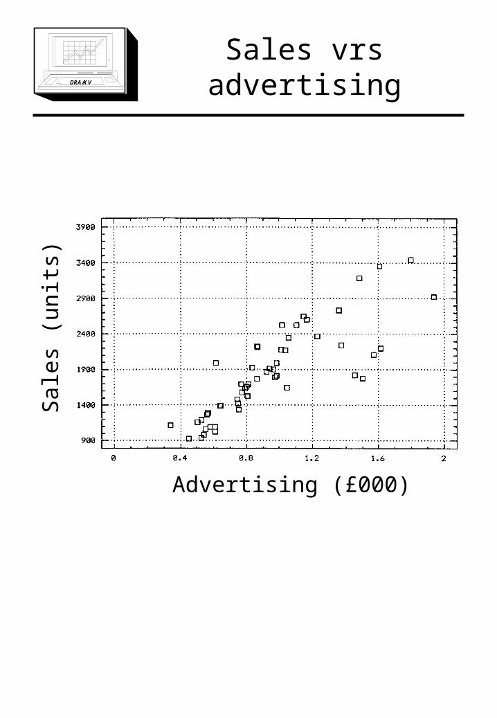
Sales vrs advertising

Advertising (£000)

Sal

es (

unit

s)

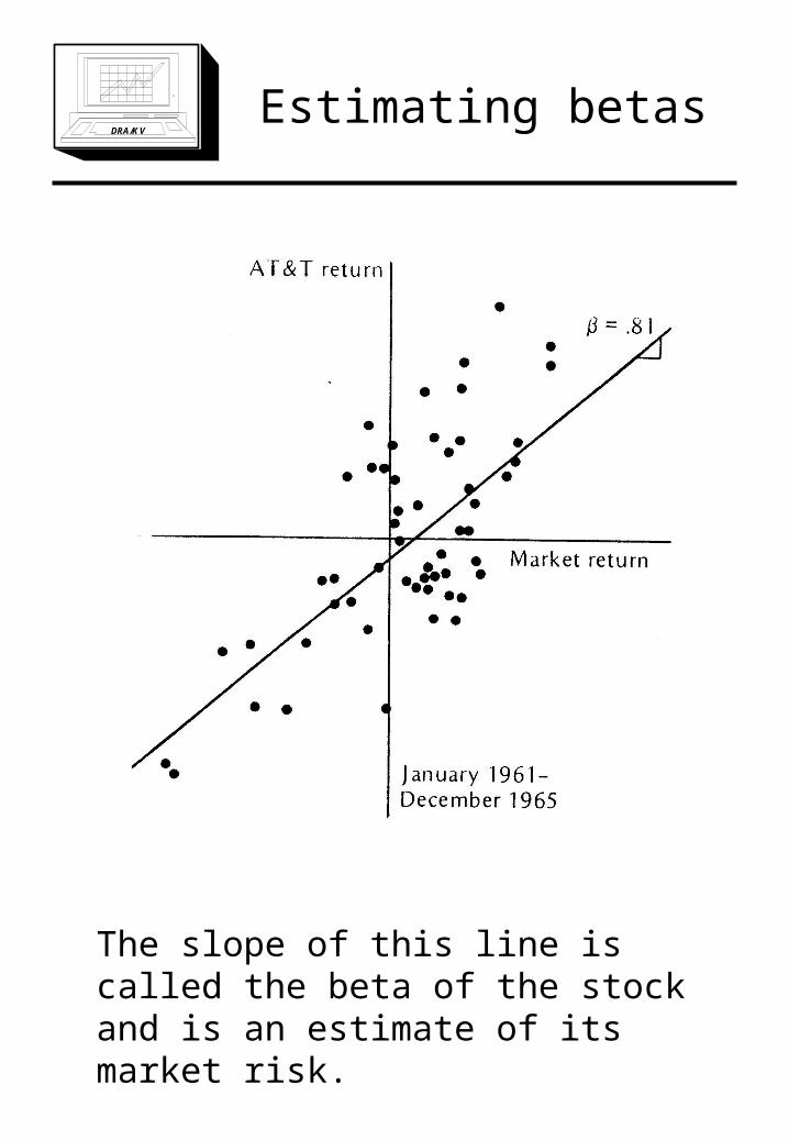
DRA/KVEstimating betas

The slope of this line is called the beta of the stock and is an estimate of its market risk.

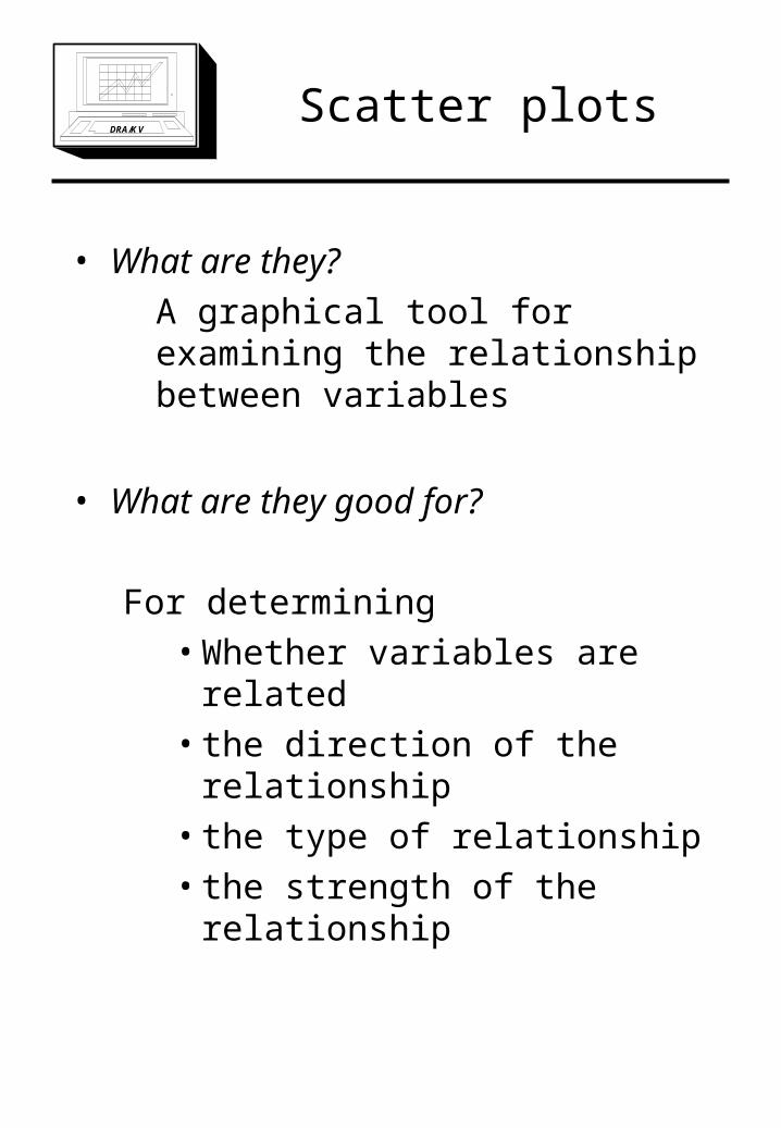
DRA/KVScatter plots

• What are they?

A graphical tool for examining the relationship between variables

• What are they good for?

For determining• Whether variables are related• the direction of the relationship• the type of relationship• the strength of the relationship

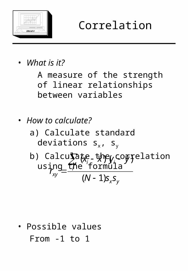
DRA/KVCorrelation

• What is it?

A measure of the strength of linear relationships between variables

• How to calculate?

a) Calculate standard deviations sx, sy

b) Calculate the correlation using the formula

• Possible values

From -1 to 1

yx

iii

xy ssN

yyxxr

)1(

))((

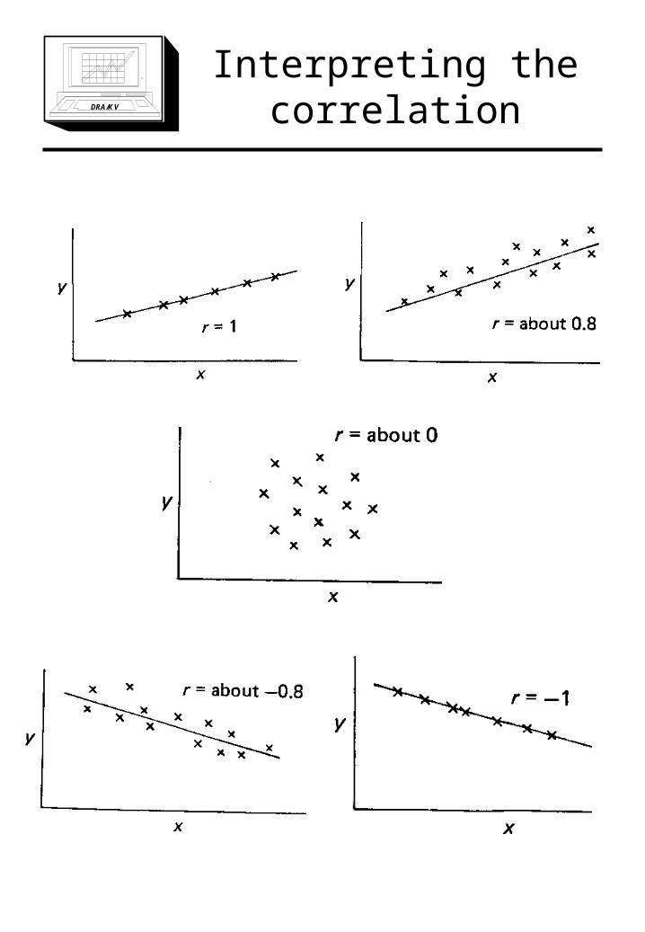
DRA/KV

Interpreting the correlation

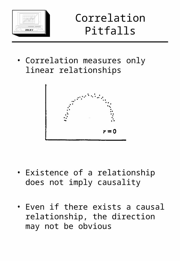
DRA/KVCorrelation Pitfalls

• Correlation measures only linear relationships

• Existence of a relationship does not imply causality

• Even if there exists a causal relationship, the direction may not be obvious

DRA/KV

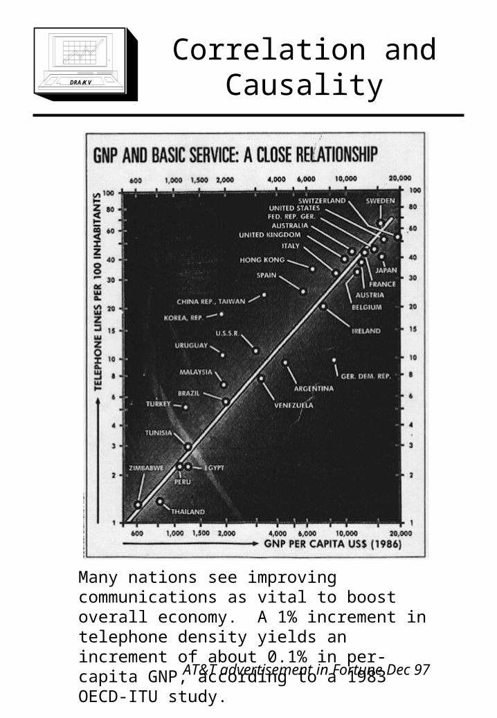
Correlation and Causality

Many nations see improving communications as vital to boost overall economy. A 1% increment in telephone density yields an increment of about 0.1% in per-capita GNP, according to a 1983 OECD-ITU study.

AT&T advertisement in Fortune Dec 97

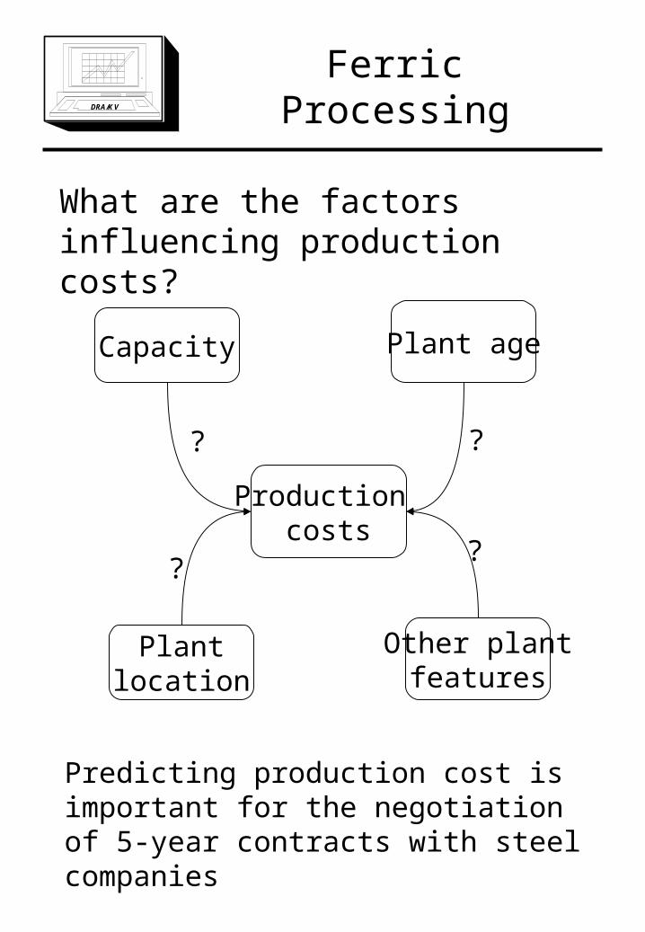
DRA/KVFerric Processing

What are the factors influencing production costs?

Production costs

Capacity Plant age

Plantlocation

Other plantfeatures

Predicting production cost is important for the negotiation of 5-year contracts with steel companies

?

? ?

?

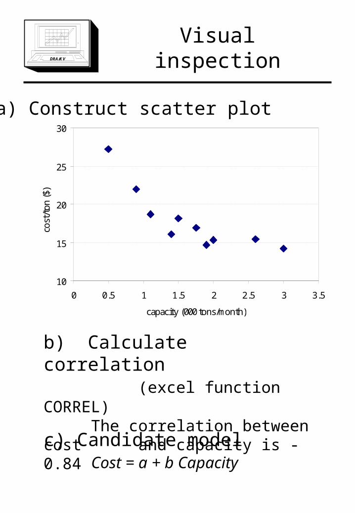
DRA/KVVisual inspection

10

15

20

25

30

0 0.5 1 1.5 2 2.5 3 3.5

capacity (000 tons/month)

cost

/ton

($)

a) Construct scatter plot

b) Calculate correlation (excel function CORREL)

The correlation between cost and capacity is -0.84

c) Candidate modelCost = a + b Capacity

DRA/KV

Simple Linear Regression

10

15

20

25

30

0 0.5 1 1.5 2 2.5 3 3.5


cost

/ton

($)

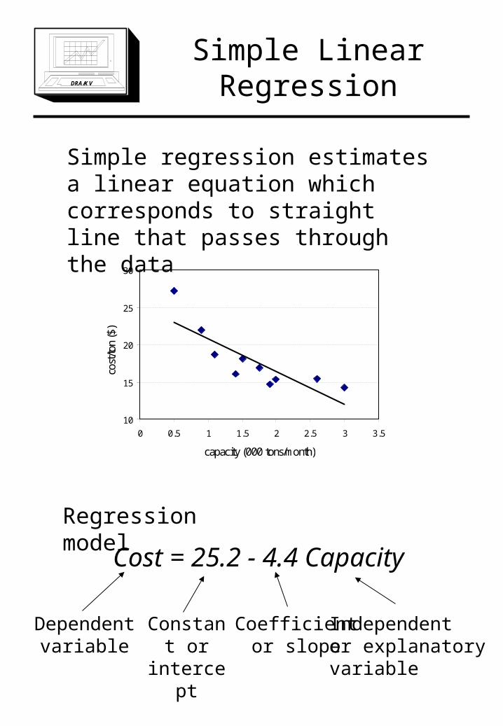
Simple regression estimates a linear equation which corresponds to straight line that passes through the data

Regression model

Cost = 25.2 - 4.4 Capacity

Dependent variable

Constant orintercept

Coefficientor slope

Independentor explanatoryvariable

DRA/KVLeast squares

10

15

20

25

30

0 0.5 1 1.5 2 2.5 3 3.5


cost

/ton

($)

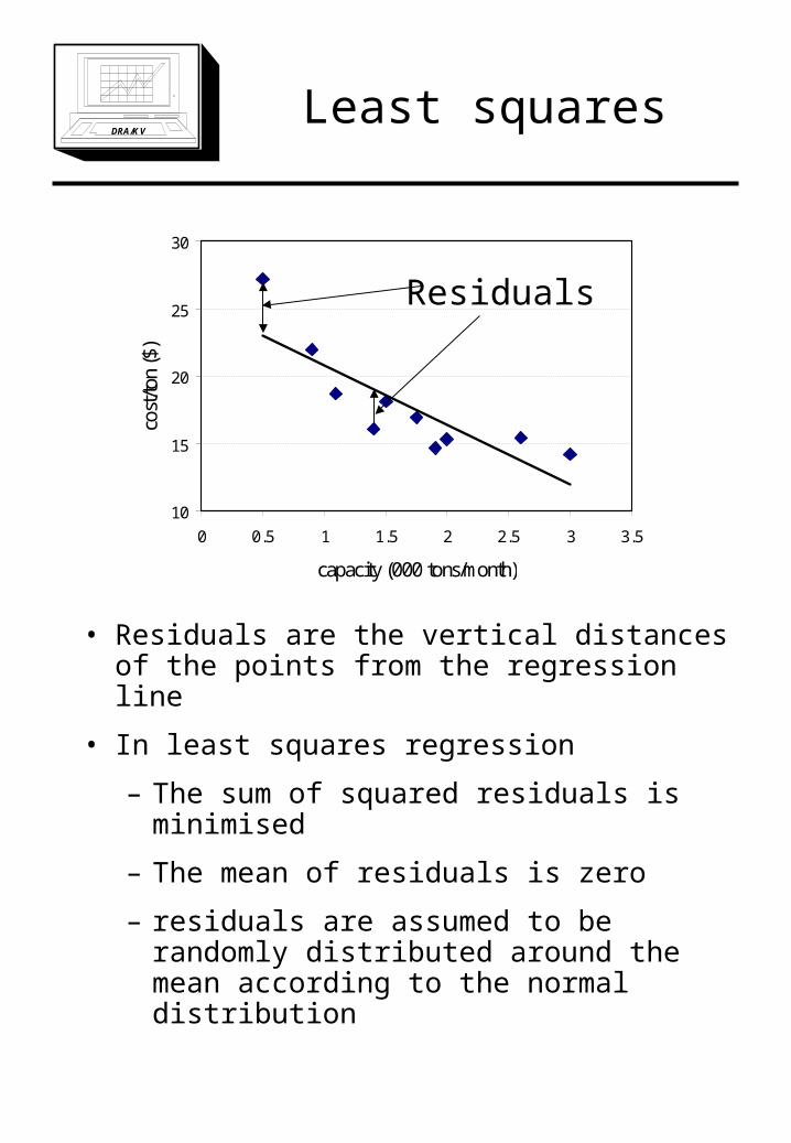
Residuals

• Residuals are the vertical distances of the points from the regression line

• In least squares regression

– The sum of squared residuals is minimised

– The mean of residuals is zero

– residuals are assumed to be randomly distributed around the mean according to the normal distribution

DRA/KVExcel output

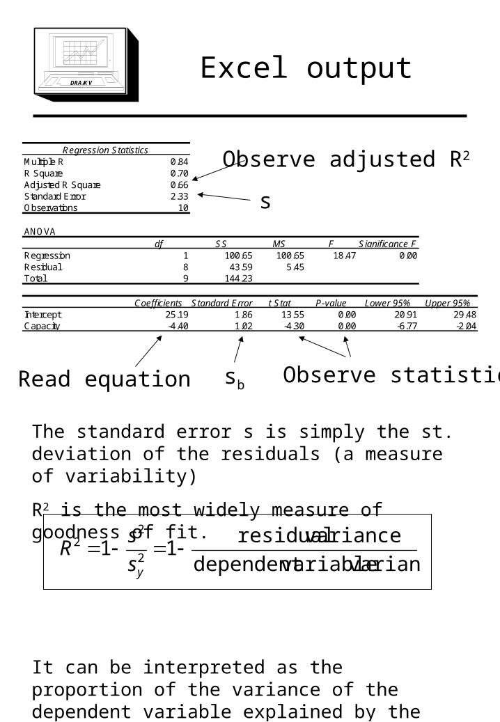
Regression StatisticsMultiple R 0.84R Square 0.70Adjusted R Square 0.66Standard Error 2.33Observations 10

ANOVAdf SS MS F Significance F

Regression 1 100.65 100.65 18.47 0.00Residual 8 43.59 5.45Total 9 144.23

Coefficients Standard Error t Stat P-value Lower 95% Upper 95%Intercept 25.19 1.86 13.55 0.00 20.91 29.48Capacity -4.40 1.02 -4.30 0.00 -6.77 -2.04

Read equation

Observe adjusted R2

Observe statisticssb

s

The standard error s is simply the st. deviation of the residuals (a measure of variability)

R2 is the most widely measure of goodness of fit.

It can be interpreted as the proportion of the variance of the dependent variable explained by the model. Use the adjusted R2 ,which accounts for the no. of observations.

variancevariabledependent

varianceresidual11

2

22

ys

sR

DRA/KVHypothesis testing

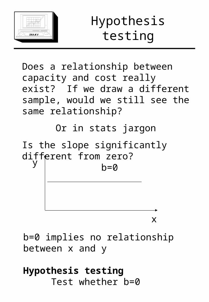
Does a relationship between capacity and cost really exist? If we draw a different sample, would we still see the same relationship?

Or in stats jargon

Is the slope significantly different from zero?

x

y b=0

b=0 implies no relationship between x and y

Hypothesis testingTest whether b=0

DRA/KV

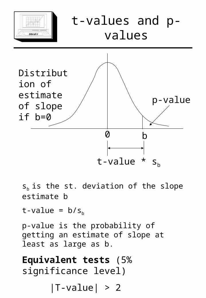
t-values and p-values

0 b

p-value

t-value * sb

sb is the st. deviation of the slope estimate b

t-value = b/sb

p-value is the probability of getting an estimate of slope at least as large as b.

Equivalent tests (5% significance level)

|T-value| > 2

p-value < 0.05

Distribution of estimate of slope if b=0

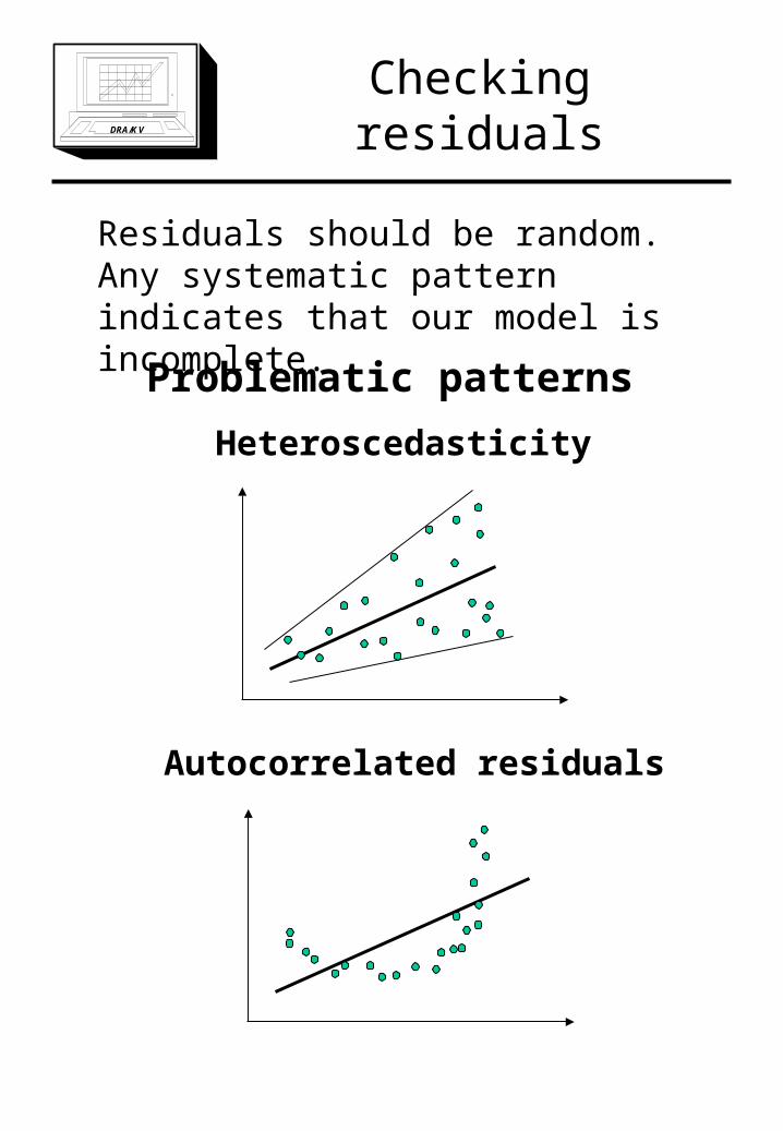
DRA/KVChecking residuals

Residuals should be random. Any systematic pattern indicates that our model is incomplete.

Autocorrelated residuals

Heteroscedasticity

Problematic patterns

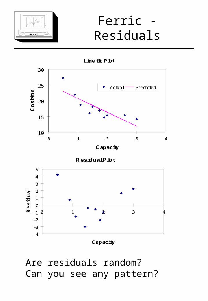
DRA/KVFerric - Residuals

Line fit Plot

10

15

20

25

30

0 1 2 3 4

Capacity

Co

st/

ton

Actual Predicted

Residual Plot

-4

-3

-2

-1

0

1

2

3

4

5

0 1 2 3 4

Capacity

Re

sid

ua

ls

Are residuals random?Can you see any pattern?

DRA/KV

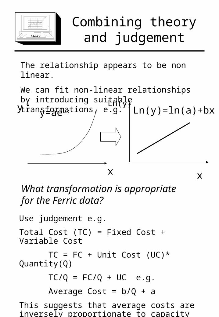
Combining theory and judgement

The relationship appears to be non linear.

We can fit non-linear relationships by introducing suitable transformations, e.g.

x

y y=aebx

x

Ln(y)Ln(y)=ln(a)+bx

What transformation is appropriate for the Ferric data?

Use judgement e.g.

Total Cost (TC) = Fixed Cost + Variable Cost

TC = FC + Unit Cost (UC)* Quantity(Q)

TC/Q = FC/Q + UC e.g.

Average Cost = b/Q + a

This suggests that average costs are inversely proportionate to capacity

DRA/KV

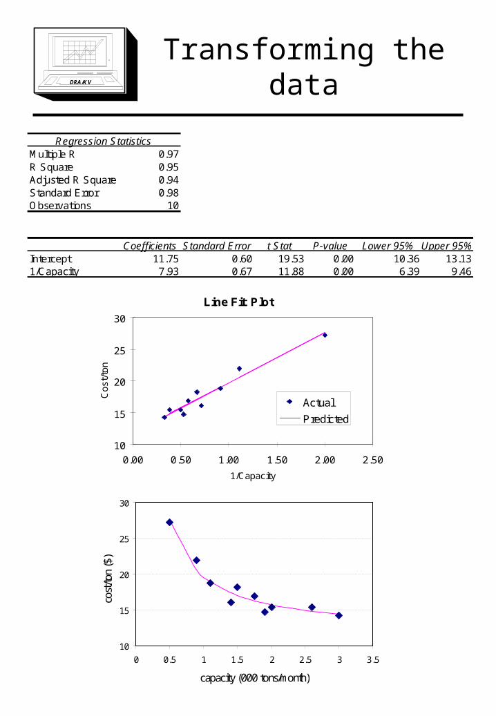
Transforming the data


Coefficients Standard Error t Stat P-value Lower 95% Upper 95%Intercept 11.75 0.60 19.53 0.00 10.36 13.131/Capacity 7.93 0.67 11.88 0.00 6.39 9.46

10

15

20

25

30

0 0.5 1 1.5 2 2.5 3 3.5


cost

/ton

($)

Line Fit Plot

10

15

20

25

30

0.00 0.50 1.00 1.50 2.00 2.50

1/Capacity

Cos

t/to

n

Actual

Predicted

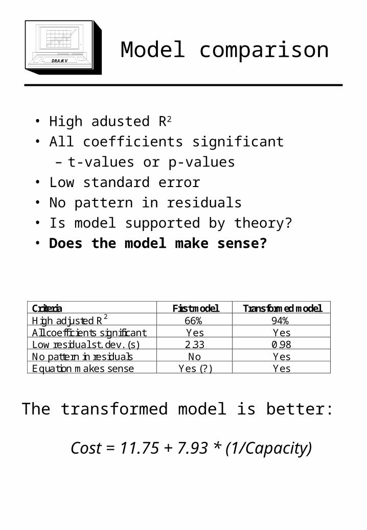
DRA/KVModel comparison

• High adusted R2

• All coefficients significant– t-values or p-values

• Low standard error• No pattern in residuals• Is model supported by theory?• Does the model make sense?

Criteria First model Transformed modelHigh adjusted R2 66% 94%All coefficients significant Yes YesLow residual st. dev. (s) 2.33 0.98No pattern in residuals No YesEquation makes sense Yes (?) Yes

The transformed model is better:

Cost = 11.75 + 7.93 * (1/Capacity)

DRA/KV

Forecasting &confidence intervals

• If capacity is 2 what is the forecast for cost?– Cost = 11.75 + 7.93 (1/2) = 15.71

• Approximate 95% confidence interval:

15.71 2 * s

where s=0.98 is the standard error

• The greater the number of observations the better the approximation

• More accurate intervals can be calculated using statistical packages

DRA/KV

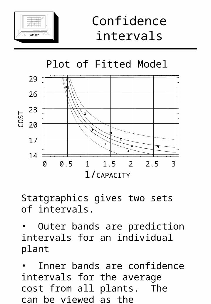
Confidence intervals

Plot of Fitted Model

1/CAPACITY

CO

ST

0 0.5 1 1.5 2 2.5 314

17

20

23

26

29

Statgraphics gives two sets of intervals.

• Outer bands are prediction intervals for an individual plant

• Inner bands are confidence intervals for the average cost from all plants. The can be viewed as the confidence intervals for the regression line.

DRA/KV

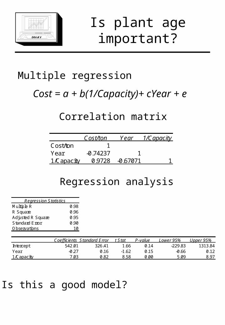
Is plant age important?

Multiple regression

Cost = a + b(1/Capacity)+ cYear + e


Coefficients Standard Error t Stat P-value Lower 95% Upper 95%Intercept 542.01 326.41 1.66 0.14 -229.83 1313.84Year -0.27 0.16 -1.62 0.15 -0.66 0.121/Capacity 7.03 0.82 8.58 0.00 5.09 8.97

Cost/ton Year 1/CapacityCost/ton 1Year -0.74237 11/Capacity 0.9728 -0.67071 1

Correlation matrix

Regression analysis

Is this a good model?

DRA/KVMulticollinearity

87878685

8585

84

83

81

81

10

15

20

25

30

0 1 2 3 4


cost

/ton

($)

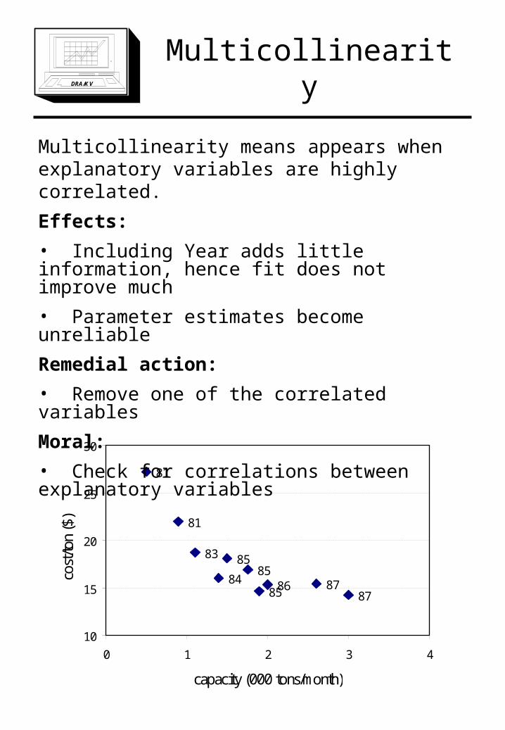
Multicollinearity means appears when explanatory variables are highly correlated.

Effects:

• Including Year adds little information, hence fit does not improve much

• Parameter estimates become unreliable

Remedial action:

• Remove one of the correlated variables

Moral:

• Check for correlations between explanatory variables

DRA/KV

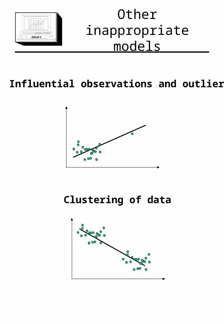
Other inappropriate models

Influential observations and outliers

Clustering of data

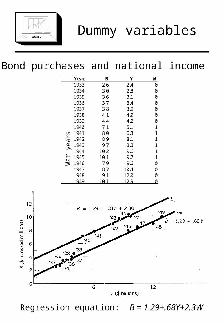
DRA/KVDummy variables

Bond purchases and national incomeYear B Y W1933 2.6 2.4 01934 3.0 2.8 01935 3.6 3.1 01936 3.7 3.4 01937 3.8 3.9 01938 4.1 4.0 01939 4.4 4.2 01940 7.1 5.1 11941 8.0 6.3 11942 8.9 8.1 11943 9.7 8.8 11944 10.2 9.6 11945 10.1 9.7 11946 7.9 9.6 01947 8.7 10.4 01948 9.1 12.0 01949 10.1 12.9 0

War

ye

ars

Regression equation: B = 1.29+.68Y+2.3W

DRA/KV

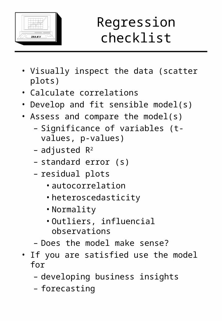
Regression checklist

• Visually inspect the data (scatter plots)

• Calculate correlations

• Develop and fit sensible model(s)

• Assess and compare the model(s)

– Significance of variables (t-values, p-values)

– adjusted R2

– standard error (s)

– residual plots

• autocorrelation

• heteroscedasticity

• Normality

• Outliers, influencial observations

– Does the model make sense?

• If you are satisfied use the model for

– developing business insights

– forecasting

DRA/KV

Preparation for Regression workshop

• Work on Excel regression tutorial

• Revise Ferric case

• Read note on Regression Analysis

• Select your workshop partner

• In preparation for the exam work on

regression exercises

Decision and Risk Analysis Regression analysis Kiriakos Vlahos Spring 99.

Documents

Transcript of Decision and Risk Analysis Regression analysis Kiriakos Vlahos Spring 99.