Decision Analysis Framework for Risk Management of Crude ... faculteit/Afdelingen... · Decision...

Hindawi Publishing CorporationAdvances in Decision SciencesVolume 2011, Article ID 456824, 17 pagesdoi:10.1155/2011/456824

Research ArticleDecision Analysis Framework for RiskManagement of Crude Oil Pipeline System

Alex W. Dawotola, P. H. A. J. M. van Gelder, and J. K. Vrijling

Hydraulic Engineering Section, Delft University of Technology, Stevinweg 1,2628 CN Delft, The Netherlands

Correspondence should be addressed to Alex W. Dawotola, [email protected]

Received 27 August 2011; Revised 11 October 2011; Accepted 26 October 2011

Academic Editor: Omer Benli

Copyright q 2011 Alex W. Dawotola et al. This is an open access article distributed under theCreative Commons Attribution License, which permits unrestricted use, distribution, andreproduction in any medium, provided the original work is properly cited.

A model is constructed for risk management of crude pipeline subject to rupture on the basis of amethodology that incorporates structured expert judgment and analytic hierarchy process (AHP).The risk model calculates frequency of failure and their probable consequences for differentsegments of crude pipeline, considering various failure mechanisms. Specifically, structured expertjudgment is used to provide frequency of failure assessments for identified failure mechanismsof the pipeline. In addition, AHP approach is utilized to obtain relative failure likelihood forattributes of failure mechanisms with very low probability of occurrence. Finally, the expected costof failure for a given pipeline segment is estimated by combining its frequency of failure and theconsequences of failure, estimated in terms of historical costs of failure from the pipeline operator’sdatabase. A real-world case study of a crude pipeline is used to demonstrate the application of theproposed methodology.

1. Introduction

1.1. Background

Pipelines carry products that are very vital to the sustenance of national economies andremain a reliable means of transporting water, oil, and gas in the world. They are generallyperceived as safe with limited number of failures recorded over their service life. However,like any other engineering assets, pipelines are subject to different degrees of failure anddegradation. When it occurs, pipeline rupture can be fatal and very disastrous. It is thereforeimportant that they are effectively monitored for optimal operation while reducing failuresto acceptable safety limit.

Integrity maintenance of pipelines is a major challenge of service companies, especiallythose involved in the transmission of oil and gas. Two major factors have been the drivingforce behind this challenge. These are the need to minimize costs of operation and doing

2 Advances in Decision Sciences

it without compromising on risk. The huge impact of pipeline failure on operational costshas necessitated the development of more effective risk management strategies to helpmitigate potential risks. Ideally, most pipeline operators ensure that during design stage,safety provisions are created to comply with theoretical minimum failure rate for the pipeline.Quantitative risk assessment has been a valuable tool to operators in minimizing risk as wellas complying with minimum safety requirement for engineering structures. In quantitativerisk assessment, an attempt is made to numerically determine the probabilities of rupturecaused by various failure mechanisms and the likely consequences of failure in terms ofeconomic loss, human hazards, and degradation of the environment.

Quantitative risk assessment (QRA) of pipeline networks is complex and can some-times be laborious due to the differences in the system networks. According to Huipeng[1], one approach to simplify QRA process is the use of hierarchical approach. Hierarchicalapproaches such as fault tree analysis, event tree analysis, and failure mode event analysishave found applications in risk assessment for complex structures as explained in Dhillonand Singh [2]. However, such methodologies are data intensive. The rupture of pipelinesoccurs in most countries rarely, and as such, the data of failures are often insufficient to carryout a thorough hierarchical approach. Also, when failure data are gathered, the classificationsmay not cover all the known failure mechanisms and attributes.

In this paper, a systematic approach to risk ranking and risk management of ruptureof crude pipelines is presented and applied to a case study. The pipeline is divided intothree different segments, and the level of risk for each segment was determined. Theproposed methodology involves a combination of two well-known techniques: AHP andCooke’s classical model for expert elicitation in the context of pipeline maintenance decisionsupport. Developed by Saaty [3], AHP fundamentally works by using opinions of expertsin developing priorities for alternatives and the criteria used to judge the alternatives ina system. The classical model proposed by Cooke [4] is a structured expert judgment-based approach. The model is able to provide rational probability assessments and has beensuccessfully applied to over forty-five expert elicitation case studies covering both academicand industrial areas by Cooke and Goossens [5].

In the proposed methodology, the classical model was used to obtain frequency offailure due to rupture for an existing crude pipeline system. Five failure mechanisms wereconsidered. These are external interference, corrosion, structural defects, operational errorsand other minor failures. Four of the failure mechanisms are further subdivided into attributesas follows:

(i) external interference (sabotage and mechanical damage),

(ii) corrosion (internal and external corrosion),

(iii) structural defects (construction defect and material defect),

(iv) operational errors (equipment failure and human error).

Analytic hierarchy process is then used to rank segments of pipeline riskwise byobtaining relative proportion of attributes with respect to the failure mechanisms. Themotivation for AHP was due to the realization that experts find it more difficult to estimatethe frequency of failure of failure attributes with generally low probability of occurrence.In essence, it was proposed to conduct pairwise ranking of the attributes using AHP. Inaddition, failure costs for each failure mechanism/attribute was estimated on the basis ofhistorical failure expenditure data obtained from the pipeline company. On the account of

Advances in Decision Sciences 3

the frequency of failure and failure costs, the expected cost of failure due to rupture on eachof the pipeline segment is then calculated.

The unique feature of the approach is that two known methodologies are combined toachieve quantitative risk assessment of pipeline assets. One of the benefits of the approach isthat the level of subjectivity in AHP is reasonably reduced, since the classical model entailsperformance-based calibration of the experts. In other words, experts’ inputs are utilized onthe basis of the consistency of the experts during elicitation process. The risk assessmentresults include quantitative estimate of frequency of failure instead of relative ranks expectedfrom a stand-alone AHP. The fact that AHP’s output are ranks and not probability can be seenas a major setback to its application in risk analysis. By combining quantitative estimates fromclassical model with relative ranking from AHP, frequencies of failure of pipeline segmentscan be estimated, taking uncertainty into consideration.

The remainder of the paper is classified into four sections. Section 2 introduces andexplains the proposed classical-AHP methodology. Section 3 presents a case study of cross-country crude pipeline to illustrate the proposed methodology. Section 4 applies the fre-quency of failure and failure costs hitherto obtained in the model to provide risk managementphilosophy of pipeline segments, and Section 5 draws the conclusion. The risk-based rankingof pipeline segments is valuable to oil and gas companies in prioritizing inspection andmaintenance activities of pipelines, ranking causes of failure by severity of impact and inbudget allocation to maintenance activities. The results could also prove valuable in arrivingat a design, redesign, construction, and monitoring decision for existing and new pipelines.

2. The Classical-AHP Methodology

In the following sections, a description of analytic hierarchy process and structured expertjudgment techniques will be provided in other to provide good background for the appli-cation of the proposed methodology in quantitative risk assessment of crude pipelines.

2.1. Failure Frequency Calculation Using StructuredExpert Judgment (The Classical Model)

The classical model is a formal method for deriving the requisite weights for a linear poolof individual experts. It is a structured expert judgment elicitation approach that involvestreating expert judgments as scientific data in a formal decision process. The basic proceduresin the classical model are pre-elicitation, elicitation, and post-elicitation. The processes thatcomprise each step are summarized in Figure 1 below.

A major part of the classical model is the requirement that experts should provideinformation only on quantities which are measurable and familiar to the experts. That is,the quantities for which the experts have to provide information should be verifiable byexperiments. The expert’s uncertainty distribution is combined using performance-basedweighting derived from their responses to the seed variables. The purpose of the seed vari-ables in the model can be classified into three, namely, (i) to quantify experts’ performanceas subjective probability assessors, (ii) to enable performance-optimized combinations ofexperts’ distributions, and (iii) to evaluate and validate the combination of expert judgments.

The tool used for carrying out structured expert judgment in classical model is theso-called expert calibration software, EXCALIBUR. The software is open access and availablethrough the Risk and Environmental Modeling (REM) group of Delft University of Tech-nology, website: http://risk2.ewi.tudelft.nl. It runs on a windows program that processes


Structured expert judgment

Step IPre-elicitation

Step IIElicitation

Step IIIPostelicitation

Define case studyIdentify target variablesIdentify query variables

Identify performance variablesIdentify and select experts

Prepare elicitation documentDry run exercise

Train experts

Expert elicitation session Combine expert assessmentsDiscrepancy and robustness analysis

Probabilistic inversion analysisDocumentation

Figure 1: Expert judgment steps.

Seed realization

Seed realization

(b) Less well-calibrated and uninformative expert

(c) Badly calibrated and highly opinionated experts

(d) Weighted combination of experts

95%

95%50%5%95%50%5%

Seed realization95%5%

5%

(a) Well-calibrated, informative expert

Figure 2: Experts calibration and information: Figures (a–c) show how experts are calibrated on the basisof responses to seed questions at given quantiles. Figure (d) shows the performance-based weightedcombination of opinions of experts (a–c) on the target items.


parametric and quantile estimates for continuous uncertain quantities into final expertsweights on the basis of the classical model. In addition to processing experts structured judg-ment, EXCALIBUR supports robustness and discrepancy analysis on the results. Robustnessanalysis shows how sensitive the results are to choice of expert and choice of calibrationvariables, and discrepancy analysis shows how the experts differ from the decision maker.

In the software, calibration and information scores are combined to derive perfor-mance-based weighted combinations of uncertainty distributions of each expert. Informationis the degree to which the distribution provided by the expert is concentrated. In the clas-sical model, the amount of concentration is commonly measured by the uniform and log-uniform distributions. Calibration measures the degree to which the actual measured valuescorrespond statistically with the experts assessments. The weights of the classical model arederived from experts’ calibration and information scores, as measured on seed variables.Figure 2 is a schematic chart that shows how calibration and information are defined fordifferent experts.

2.2. Failure Likelihood Estimate Using Analytic Hierarchy Process

Analytic hierarchy process is used in the methodology to rank the attributes of failure mecha-nisms according to the likelihood of failure for different segments of the pipeline. Theoutcome is a relative scale which gives a rational basis for risk-based decision making. Ana-lytic hierarchy process has found applications in diverse industries. For example, Quresh andHarrison [6] applied AHP in Riparian revegetation policy selections for a small watershed inAustralia. Similarly, Cagno et al. [7] utilised AHP as an elicitation method of expert opinionto determine the a priori distribution of gas pipeline failures, and Dey [8] applied AHP inbenchmarking project management practices of Caribbean organizations. The building blocksof analytic hierarchy process are briefly explained below.

2.3. Procedures for Analytic Hierarchy Process

The first step of analytic hierarchy process is problem formulation, which involves the ulti-mate goal for the analysis. In the risk ranking of pipeline, the goal will be selection of pipelinesegments with the highest likelihood of rupture due to different failure mechanisms andattributes. Once the goal has been defined, the failure mechanisms are then identified. Thefailure mechanisms are further divided into attributes. The failure mechanisms and attributes willbe in the first and second level hierarchy, respectively, in the AHP value tree.

Secondly, the decision alternatives are selected. The identification of decisionalternatives is a very important procedure in analytic hierarchy process. As a matter of fact,the conclusion on the decision alternatives is the outcome of the AHP. For example, thedecision maker or an expert could be asked to conduct pairwise assessments of failure mech-anisms/attributes of pipeline rupture for a set of pipeline segments. In this case, pipelinesegments will be the decision alternatives, and the goal will be to compare these pipeline seg-ments in terms of failure, and to rank them on the basis of the perceived likelihood of rupture.

The next step is the development of hierarchy (value tree). The value tree connectstogether the goal of the risk assessment, the failure mechanisms and attributes, and the deci-sion variables. In the value tree for risk ranking of crude pipeline, the goal (pipeline selection) isconnected to the first level hierarchy (failure mechanisms). The first level hierarchy is then con-nected to the decision variables (pipeline segments) via the second level hierarchy (attributes).


Table 1: Scale of decision preference for comparing two failure attributes.

Judgment Explanation Score

Equally Two attributes have equal likelihood of rupture 1

Moderately The likelihood of rupture due to one attribute is slightly morethan the other attribute 3

Strongly The likelihood of rupture due to one attribute is stronglymore than the other attribute 5

Very strongly The likelihood of rupture due to one attribute is very stronglymore than the other attribute 7

Extremely The likelihood of rupture due to one attribute is extremelymore than the other attribute 9

Intermediate judgment The intermediate values are used when compromise is needed 2, 4, 6, 8

Thirdly, all necessary information pertaining to the pipeline segments will be collectedand recorded. To aid in the classification of the segments, the required features could bedivided into physical data, construction data, operational data, inspection data, and failurehistory. The necessary information on the pipeline/segments should be documented andmade available to the experts before pairwise ranking exercise.

Finally, a training session should be organized to familiarize experts with the elic-itation procedures. During the elicitation, the experts rank each pair of attribute on the basisof scale proposed by Saaty [3]. Table 1 below gives an explanation of the scale for com-paring two attributes. For example, if two criteria are judged to have the same level of risk,the pairwise comparison score will be 1. A score of 9 is given if one criterion is assumed to beextremely stronger than the other. Intermediate judgments of 2, 4, 6, and 8 are selected whena conclusion cannot be reached from the scores of 1, 3, 5, and 7 as defined in Table 1. Theresponses are consolidated in a preference matrix and synthesized to obtain the weightages.

2.3.1. Consistency Check

AHP provides the possibility of checking the logical consistency of the pairwise matrix bycalculating the consistency ratio (CR). The acceptable value for CR is 0.1 maximum, indi-cating deviations from nonrandom entries of less than an order of magnitude. Factors thataffect consistency ratio include homogeneity of attributes of the decision variables, sparsenessof the attributes, and the level of knowledge of experts participating in the pairwise rankingof attributes.Given a weight vector,

�w =

⎡⎢⎢⎣w1

w2

wn

⎤⎥⎥⎦. (2.1)

Obtained from a decision matrix,

A =

⎡⎢⎢⎣a11 a12 a1n

a21 a22 a2n

an1 an2 ann

⎤⎥⎥⎦. (2.2)


The consistency of the decision matrix is calculated as follows: multiply matrix A by theweight vector �w to give vector,

�B = �A · �w =

⎡⎢⎢⎣b1

b2

bn

⎤⎥⎥⎦, (2.3)

where

b1 = a11w1 + a12w2 + a1nwn,

b2 = a21w1 + a22w2 + a2nwn,

bn = an1w1 + an2w2 + annwn.

(2.4)

Divide each element of vector, �B with the corresponding element in the weight vector �w togive a new vector

c =

⎡⎢⎢⎣b1/w1

b2/w2

bn/wn

⎤⎥⎥⎦ =

⎡⎢⎢⎣c1

c2

cn

⎤⎥⎥⎦, (2.5)

λmax is the average of the elements of vector �c:

λmax =1n

n∑i=1

ci. (2.6)

Consistency Index is then calculated using,

CI =λmax − n

n − 1, (2.7)

where n is order of the decision matrix and λmax is obtained from (2.6) above.Using (2.7), consistency ratio is calculated as

CR =CIRI

, (2.8)

where RI is the random index and its value is obtained from Table 2 below.Other measures of consistency have been defined. For example, Mustajoki J and

Hamalainen [9] give a consistency measure (CM) of between 0 to 1 using the multiattributevalue theory inherent in their Web-HIPRE software. According to their work, a CM of 0.2 isconsidered acceptable.


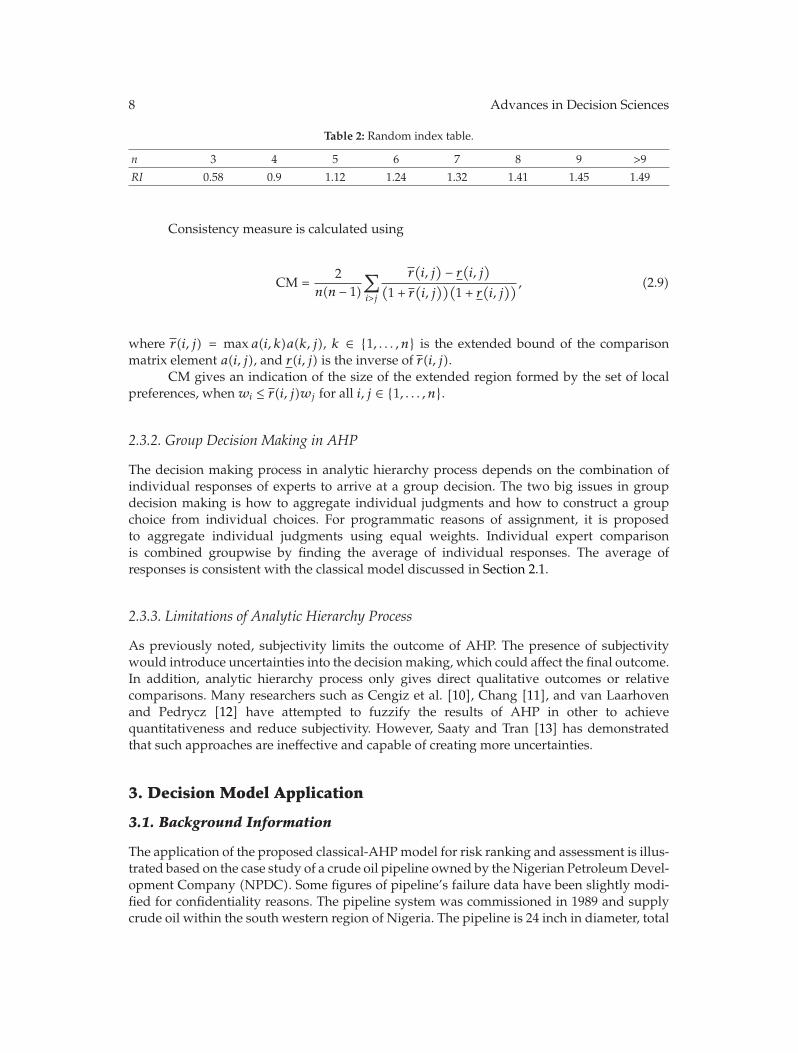
Table 2: Random index table.

n 3 4 5 6 7 8 9 >9

RI 0.58 0.9 1.12 1.24 1.32 1.41 1.45 1.49

Consistency measure is calculated using

CM =2

n(n − 1)

∑i>j

r(i, j

) − r(i, j

)(1 + r

(i, j

))(1 + r

(i, j

)) , (2.9)

where r(i, j) = maxa(i, k)a(k, j), k ∈ {1, . . . , n} is the extended bound of the comparisonmatrix element a(i, j), and r(i, j) is the inverse of r(i, j).

CM gives an indication of the size of the extended region formed by the set of localpreferences, when wi ≤ r(i, j)wj for all i, j ∈ {1, . . . , n}.

2.3.2. Group Decision Making in AHP

The decision making process in analytic hierarchy process depends on the combination ofindividual responses of experts to arrive at a group decision. The two big issues in groupdecision making is how to aggregate individual judgments and how to construct a groupchoice from individual choices. For programmatic reasons of assignment, it is proposedto aggregate individual judgments using equal weights. Individual expert comparisonis combined groupwise by finding the average of individual responses. The average ofresponses is consistent with the classical model discussed in Section 2.1.

2.3.3. Limitations of Analytic Hierarchy Process

As previously noted, subjectivity limits the outcome of AHP. The presence of subjectivitywould introduce uncertainties into the decision making, which could affect the final outcome.In addition, analytic hierarchy process only gives direct qualitative outcomes or relativecomparisons. Many researchers such as Cengiz et al. [10], Chang [11], and van Laarhovenand Pedrycz [12] have attempted to fuzzify the results of AHP in other to achievequantitativeness and reduce subjectivity. However, Saaty and Tran [13] has demonstratedthat such approaches are ineffective and capable of creating more uncertainties.

3. Decision Model Application

3.1. Background Information

The application of the proposed classical-AHP model for risk ranking and assessment is illus-trated based on the case study of a crude oil pipeline owned by the Nigerian Petroleum Devel-opment Company (NPDC). Some figures of pipeline’s failure data have been slightly modi-fied for confidentiality reasons. The pipeline system was commissioned in 1989 and supplycrude oil within the south western region of Nigeria. The pipeline is 24 inch in diameter, total


length 340 km, with design pressure and operating temperature of 100 bar and 26.8◦C, respec-tively. The material of the pipeline is made from API5LX42 carbon steel, with a concrete typecoating. It is basically located onshore but connects a compressor station located offshore.

In the analysis, the entire pipeline is classified into three segments (X1, X2, and X3), inline with its natural stretch. AHP-classical model is utilized to assess the risks related to thepipeline by arranging the segments of pipeline into a hierarchical ranking of risk. The aimof the analysis is to prioritize the most critical segments of pipeline to various failure mech-anisms due to rupture. The analysis also takes into consideration the human, environmental,and financial consequences of accidents which may occur in any segment of pipeline.

In order to start the analysis, six pipeline experts from the company were invitedand trained on the application of the model. Failure data sheet of each pipeline segment ismade available to the experts. The failure data sheet contains information related to pipelinerepair history, design parameters, inspection records, and current operating conditions.All the experts are familiar with the pipeline and pipeline segments under study. Theyparticipated in both structured expert judgment and AHP-based pairwise ranking of thepipeline segments. The procedure is explained separately below.

3.2. Estimation of Failure Frequency Using the Classical Model

Estimation of failure frequencies and uncertainties is carried out on the basis of the classicalmodel. Five failure mechanisms were considered for each pipeline segment, namely, externalinterference, corrosion, structural defects, operational errors, and other minor failures. Thefailure mechanisms are actually the target variables in the classical model. In total, twentyeight variables were obtained, considering five target variables for each segment of thepipeline and ten seed variables that are used to calibrate the experts. The seed variableswere obtained using generic equipment failure rates from literature and books to calibratethe experts. Initially, the experts were elicitated on the values of the seed variables. Thereafter,each of the experts was required to provide 5%, 50%, and 95% quantiles of the uncertaintydistributions for the frequency of failure (in kmyr) by rupture due to the failure mechanismsfor segment X1, X2, and X3 of the pipeline.

3.2.1. Expert Calibration

The experts’ responses were processed using EXCALIBUR software. The outcome of expertcalibration which is based on performance of the “seed” variables are displayed in Table 3.The optimal decision maker (ODM) is also computed. The ODM is obtained as thenormalized weighted linear combination of the experts’ distributions. In EXCALIBUR, theexperts’ distributions can be combined using either global weight, item weight, or equal weight.However, in this paper, global weight was used, because it possesses the best calibration andunnormalized weight—which is the combined score of the experts.

From Table 3, the calibration of the experts reveals that the best experts (in anincreasing order) are experts 1, 6, and 4 with normalized weights of 0.248, 0.30, and 0.452respectively. The other experts (2, 3, and 5) have very low calibration scores, and theirindividual weights are not considered in the optimal decision maker. Therefore, only experts1, 6, and 4 form the decision maker. The calibration and information of the optimal decisionmaker is calculated on the basis of global weight, as discussed before. The outcome confirmsthe assertion that the ODM calculated on the basis of global weight (calibration = 0.474)


Table 3: Results of expert calibration and optimal decision maker.

Expert Calibration Relative informationrealization Unnormalized weight Normalized weight DM

1 0.036 2.968 0.106 0.2482 0 3.738 0 03 0.001 2.201 0 04 0.101 1.906 0.193 0.4525 0 2.553 06 0.036 3.584 0.128 0.300Global DM 0.474 1.606 0.761Item DM 0.290 1.853 0.537Equal DM 0.114 0.989 0.112

Table 4: Robustness analysis of the experts.

Excluded expert Information to backgroundrealization Calibration Information to original DM

realization

1 1.323 0.550 0.2852 1.606 0.474 0.0013 1.082 0.474 0.0524 2.426 0.244 0.8245 1.199 0.474 0.0386 1.238 0.474 0.278None 1.606 0.474 0

possess the best calibration than item weight-based decision maker (calibration = 0.29) andequal weight based decision maker (calibration = 0.11). In addition, it is found that the ODMis better calibrated and its unnormalized weight dominates that of the best experts (1, 4, and6). However, on the basis of relative information realization, it can be said that the decisionmaker is less informative than the best experts.

3.2.2. Robustness Analysis

Robustness analysis is performed on the seed variables and the experts. In the robustnessanalysis, the variables of interest are removed one at a time, and the analysis is repeated untilall variables have been covered. The robustness analysis on the experts shown in Table 4indicates that the calibration score for the experts range from 0.474 to 0.55. These scores arewell above the calibration score of 0.29 and 0.114 obtained for the item weight DM (itemDM) and equal weight DM (equal DM), respectively, in Table 3. Similarly, the robustness ofthe seed variables is analysed and found to range from 0.405 to 0.731 (Table 5). The initialcalibration score obtained for the global DM in Table 3 was 0.474. The analysis confirmsthe robustness of both the experts and the seed variables, when calibration and informationscores of the new decision makers (Tables 4 and 5) are compared with that of the originaldecision maker (Table 3).


Table 5: Robustness analysis of the seed items.

Excluded seedvariable Information to background realization Calibration Information to original DM

realization

1 1.129 0.405 0.5492 1.569 0.571 0.1943 1.701 0.405 0.2274 1.132 0.571 0.1675 2.452 0.593 0.8216 1.179 0.731 0.7377 0.958 0.571 0.5938 1.626 0.405 0.0959 1.346 0.571 0.28710 1.804 0.405 0.133None 1.606 0.474 0

3.2.3. Resulting Solution

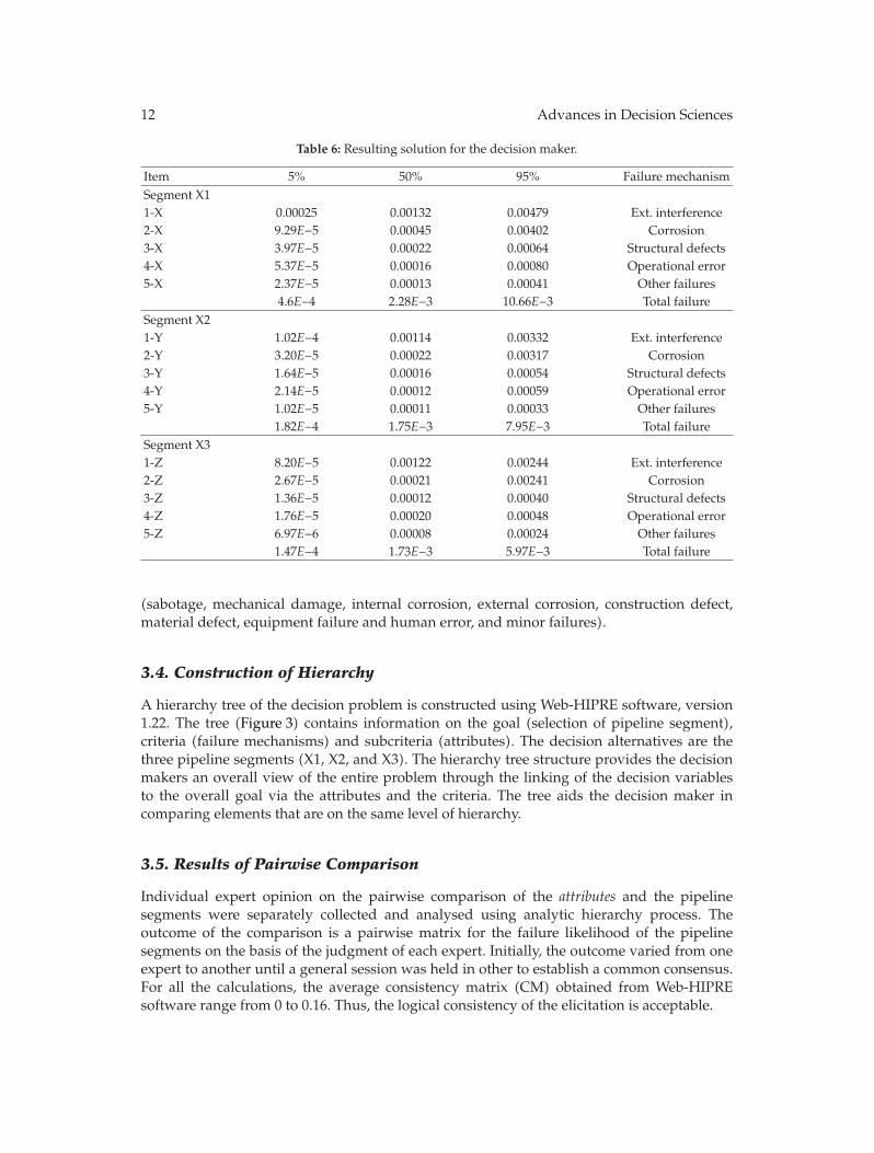
The resulting solution is the combined decision maker’s distribution of values assessed byexperts that contribute to the ODM. The DM optimization is achieved at a significance levelof 0.0358, giving 96.4% acceptable level. The acceptance level is acceptable and the outcome ofthe structured expert judgment on the frequency of failure of the pipeline due to the identifiedfailure mechanisms for the segments of the pipeline (X1, X2, and X3) is satisfactory. Detailedresults of the calculation of failure frequencies are given in Table 6. The 50% uncertaintyfrequencies of failure for segments X1, X2, and X3 are 2.28E−3 per kmyr, 1.75E−3 per kmyr,and 1.73E−3 per kmyr, respectively.

The overall failure frequencies compare favourably with results reported in literatures.For example, Little [14] reported a value of 0.42E−3 per kmyr for frequency of failure inWestern Europe petroleum pipelines, 0.3E−3 per kmyr for cross country oil pipelines in UnitedKingdom, and 0.53E−3 per kmyr for total failure of USA Department of Transportation’s liquidpipelines. The difference between these values and the frequency of failure obtained for thecase study could be due to factors such as difference in location and physical and processproperties of the pipelines. These factors have been shown to have significant influence onfrequency of failure of pipelines, according to Restrepo et al. [15].

From Table 6, using 50% quantile estimate, it appears that X1 is the most vulnerableamong the three pipeline segments, having the highest frequency of failure, followed by X2and then X3. However, it is interesting to note that X3 has the highest frequency of failure dueto operational error. This can be explained partially by the fact that there are more controlvalves that involve manual operations in X3 compared to X1 and X2.

3.3. Relative Estimate of Failure Attributes

In this step, AHP is utilized to determine the likelihood of rupture due to the failure attributes.The six experts that participated in the study were provided with questionnaires that describefeatures of pipeline segments X1, X2, and X3. The questionnaires were formulated so as toselect pipeline segment on the basis of risk of rupture, considering all the failure attributes


Table 6: Resulting solution for the decision maker.

Item 5% 50% 95% Failure mechanismSegment X11-X 0.00025 0.00132 0.00479 Ext. interference2-X 9.29E−5 0.00045 0.00402 Corrosion3-X 3.97E−5 0.00022 0.00064 Structural defects4-X 5.37E−5 0.00016 0.00080 Operational error5-X 2.37E−5 0.00013 0.00041 Other failures

4.6E−4 2.28E−3 10.66E−3 Total failureSegment X21-Y 1.02E−4 0.00114 0.00332 Ext. interference2-Y 3.20E−5 0.00022 0.00317 Corrosion3-Y 1.64E−5 0.00016 0.00054 Structural defects4-Y 2.14E−5 0.00012 0.00059 Operational error5-Y 1.02E−5 0.00011 0.00033 Other failures

1.82E−4 1.75E−3 7.95E−3 Total failureSegment X31-Z 8.20E−5 0.00122 0.00244 Ext. interference2-Z 2.67E−5 0.00021 0.00241 Corrosion3-Z 1.36E−5 0.00012 0.00040 Structural defects4-Z 1.76E−5 0.00020 0.00048 Operational error5-Z 6.97E−6 0.00008 0.00024 Other failures

1.47E−4 1.73E−3 5.97E−3 Total failure

(sabotage, mechanical damage, internal corrosion, external corrosion, construction defect,material defect, equipment failure and human error, and minor failures).

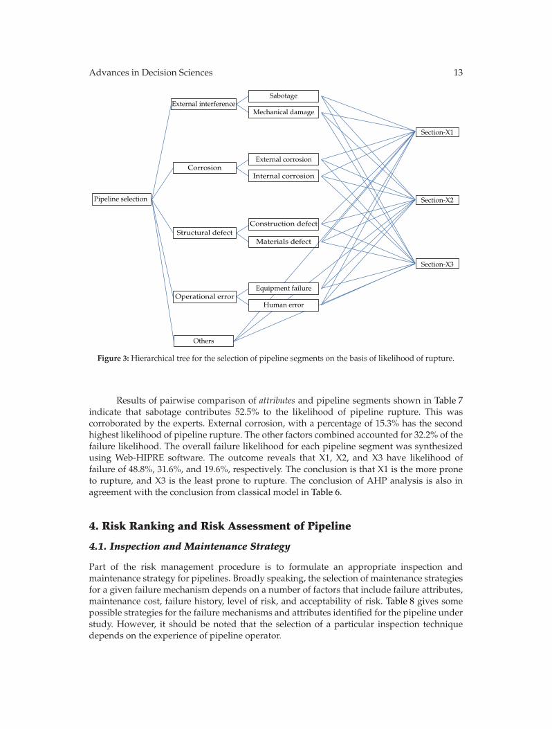
3.4. Construction of Hierarchy

A hierarchy tree of the decision problem is constructed using Web-HIPRE software, version1.22. The tree (Figure 3) contains information on the goal (selection of pipeline segment),criteria (failure mechanisms) and subcriteria (attributes). The decision alternatives are thethree pipeline segments (X1, X2, and X3). The hierarchy tree structure provides the decisionmakers an overall view of the entire problem through the linking of the decision variablesto the overall goal via the attributes and the criteria. The tree aids the decision maker incomparing elements that are on the same level of hierarchy.

3.5. Results of Pairwise Comparison

Individual expert opinion on the pairwise comparison of the attributes and the pipelinesegments were separately collected and analysed using analytic hierarchy process. Theoutcome of the comparison is a pairwise matrix for the failure likelihood of the pipelinesegments on the basis of the judgment of each expert. Initially, the outcome varied from oneexpert to another until a general session was held in other to establish a common consensus.For all the calculations, the average consistency matrix (CM) obtained from Web-HIPREsoftware range from 0 to 0.16. Thus, the logical consistency of the elicitation is acceptable.


External interferenceSabotage

Mechanical damage

External corrosion

Internal corrosion

Construction defect

Materials defect

Equipment failure

Human error

Corrosion

Structural defect

Operational error

Section-X1

Pipeline selection Section-X2

Section-X3

Others

Figure 3: Hierarchical tree for the selection of pipeline segments on the basis of likelihood of rupture.

Results of pairwise comparison of attributes and pipeline segments shown in Table 7indicate that sabotage contributes 52.5% to the likelihood of pipeline rupture. This wascorroborated by the experts. External corrosion, with a percentage of 15.3% has the secondhighest likelihood of pipeline rupture. The other factors combined accounted for 32.2% of thefailure likelihood. The overall failure likelihood for each pipeline segment was synthesizedusing Web-HIPRE software. The outcome reveals that X1, X2, and X3 have likelihood offailure of 48.8%, 31.6%, and 19.6%, respectively. The conclusion is that X1 is the more proneto rupture, and X3 is the least prone to rupture. The conclusion of AHP analysis is also inagreement with the conclusion from classical model in Table 6.

4. Risk Ranking and Risk Assessment of Pipeline

4.1. Inspection and Maintenance Strategy

Part of the risk management procedure is to formulate an appropriate inspection andmaintenance strategy for pipelines. Broadly speaking, the selection of maintenance strategiesfor a given failure mechanism depends on a number of factors that include failure attributes,maintenance cost, failure history, level of risk, and acceptability of risk. Table 8 gives somepossible strategies for the failure mechanisms and attributes identified for the pipeline understudy. However, it should be noted that the selection of a particular inspection techniquedepends on the experience of pipeline operator.


Table 7: Pairwise ranking of failure criteria and likelihood.

Failure mechanisms Attributes Likelihood Pipeline segmentX1 X2 X3

External interferenceSabotage 0.525 0.271 0.179 0.076

Mechanical damage 0.081 0.051 0.019 0.011

CorrosionExternal corrosion 0.153 0.093 0.041 0.018Internal corrosion 0.061 0.009 0.021 0.031

Structural defectsConstruction defect 0.045 0.023 0.014 0.009

Materials defects 0.021 0.006 0.007 0.008

Operational errorEquipment failure 0.050 0.009 0.018 0.024

Human error 0.019 0.003 0.007 0.009

Others Others 0.044 0.023 0.011 0.010

Overall 0.488 0.316 0.196

Table 8: Maintenance strategy for pipeline failures.

Failure mechanism Attributes Maintenance strategy

External interference Sabotage PatrollingMechanical damage Pipeline marking/improved right of Way

Corrosion External corrosion Pipe coatingInternal corrosion Intelligent pigging survey

Structural defects Construction defect Reconstruction/replacementMaterials defects Replacement of pipelines

Operational error Equipment failure Replacement of faulty equipmentHuman error Operator training

4.2. Expected Failure Cost

For each pipeline segment, severity of failure was estimated from historical failure costs fromdatabase of the pipeline company. The failure costs obtained from the database could notbe used directly due to proprietary reasons. The original data was slightly adjusted, andestimates were used in the risk calculations. However, the determination of cost of failureis based on the category of failure. In the Nigerian context, the category of failure in USdollars includes small failure (less than $50,000), medium failure (between $50,000 and up to$200,000), large failure (between $200,000 and $500,000), and catastrophic failure (more than$1 million).

4.3. Risk Ranking of Pipeline Segments

In Table 9, pipeline segments X1, X2, and X3 are ranked on the basis of level of risk. The resultof frequency of failure (Table 6) shows X1 as the most vulnerable among the three segments,followed by X2 and then X3. However, when failure costs are taken into account and theexpected cost of failure is calculated (Table 9) for 50% uncertainty measure of frequency offailure, the trend changed. The system with highest risk remains X1 but X3 now ranked higherbased on expected level of risk than X2.


Table 9: Expected failure cost for pipeline segment X1, X2, and X3.

Pipelinesegment

Frequency of failure (per kmyr)Failure cost (‘$000) Expected cost of failure

(‘$000 per kmyr)Risk ranking

5% 50% 95%

X1 4.6E−4 2.28E−3 10.66E−3 5,100 11.6 1

X2 1.82E−4 1.75E−3 7.95E−3 2,095 3.67 3

X3 1.47E−4 1.73E−3 5.97E−3 2,425 4.20 2

In Table 10, the ranking obtained from AHP result in Table 7 is combined with severityof failure to calculate the expected failure cost for each pipeline segment at 50% uncertaintymeasure of frequency of failure. The expected failure cost calculation shows that the allocationof equal maintenance resources to the three segments will be a less effective maintenancestrategy, since they differ in expected cost of failure.

5. Conclusions

A decision-based model has been presented for risk ranking and risk assessment man-agement of crude oil pipelines. The model uses structured expert judgment and analytichierarchy process to predict the frequency of failure and severity of failure for a givenpipeline. The work hopes to contribute to the process of prioritizing transportation pipelinesfor integrity maintenance on the basis of the results of risk ranking and risk assessmentconducted.

The assumption in the AHP model is that each expert would have equal weightin the final decision making. However, the assumption may prevent the decision makerin reaching an optimum conclusion, since equal representation may not always lead torational consensus. We have been able to demonstrate that an optimum decision makingcan be achieved with the use of structured expert judgment on the basis of the so-calledclassical model. The classical model reveals that only three out of the six experts actuallycontribute to the optimum decision making. In addition, the subjectivity inherent in AHP canbe minimized through estimation of uncertainties in the expert elicitation.

The case study revealed some interesting conclusions, which shows that location playsa significant role in pipeline integrity as expected cost of failure vary along pipeline segments.For the case study, external interference is found to be the most important failure criterion,representing over 50% of entire failures. The high likelihood of failure by external interferenceis due to a somewhat high occurrence of sabotage acts and mechanical damage around thepipeline location. Therefore, increased surveillance along pipeline’s right of way would helpimprove pipeline reliability.

The result also confirms that equal allocation of maintenance resources to pipelinesegments may not always be the optimal maintenance decision. For example, in the allocationof maintenance resources for pipeline under study, X1, with the highest expected failurecost should receive more attention than the other segments. In addition, X3 will requiremore maintenance resources than X2. The maintenance manager will find this approach tobe beneficial in formulating the annual inspection and maintenance policy for company’sassets. Furthermore, the outcome of the decision analysis could prove useful in formulatingindividual and societal risk acceptance criteria for regulatory compliance. In general, theaccuracy of the severity of failure and the expected cost of failure calculated could be furtherimproved with more pipeline failure data.


Table

10:T

otal

risk

asse

ssm

ents

for

cros

s-co

untr

ycr

ude

oilp

ipel

ine.

Failu

rem

echa

nism

Pipe

line

segm

ent

Freq

uenc

yof

failu

re(per

kmyr)

Att

ribu

tes

Rel

ativ

era

nkFr

eque

ncy

offa

ilure

(per

kmyr)

Failu

reco

st(‘

$000)

Exp

ecte

dco

stof

failu

re(‘

$000

perkm

yr)

5%50

%95

%5%

50%

95%

Ext

erna

lin

terf

eren

ce

X1

0.00

025

0.00

132

0.00

479

Sabo

tage

0.27

12.

10E−4

1.11E−3

4.03E−3

2,20

024

44M

echa

nica

lDam

age

0.05

13.

96E−5

2.09E−4

7.59E−4

1,00

020

9.1

X2

1.02E−4

0.00

114

0.00

332

Sabo

tage

0.17

99.

22E−5

1.03E−3

3.00E−3

800

824.

5M

echa

nica

lDam

age

0.01

99.

79E−6

1.09E−4

3.19E−4

400

43.8

X3

8.20E−5

0.00

122

0.00

244

Sabo

tage

0.07

67.

16E−5

1.57E−3

2.13E−3

1,00

015

72.4

Mec

hani

calD

amag

e0.

011

1.04E−5

2.28E−4

3.09E−4

500

113.

8

Cor

rosi

on

X1

9.29E−5

0.00

045

0.00

402

Ext

erna

lcor

rosi

on0.

093

8.47

E−5

4.10E−4

3.67E−3

300

123.

1In

tern

alco

rros

ion

0.00

98.

20E−6

3.97E−5

3.55E−4

200

7.9

X2

3.20E−5

0.00

022

0.00

317

Ext

erna

lcor

rosi

on0.

041

2.12

E−5

1.45E−4

2.10E−3

120

17.5

Inte

rnal

corr

osio

n0.

021

1.08E−5

7.45E−5

1.07E−3

806.

0

X3

2.67E−5

0.00

021

0.00

241

Ext

erna

lcor

rosi

on0.

018

9.81

E−6

7.71E−5

8.85E−4

120

9.3

Inte

rnal

corr

osio

n0.

031

1.69E−5

1.33E−4

1.52E−3

100

13.3

Stru

ctur

ald

efec

ts

X1

3.97E−5

0.00

022

0.00

064

Con

stru

ctio

nd

efec

t0.

023

3.15

E−5

1.74E−4

5.08E−4

8014

.0M

ater

iald

efec

t0.

006

8.21

E−6

4.55E−5

1.32E−4

200.

9

X2

1.64E−5

0.00

016

0.00

054

Con

stru

ctio

nd

efec

t0.

014

1.09

E−5

1.07E−4

3.60E−4

303.

2M

ater

iald

efec

t0.

007

5.47

E−6

5.33E−5

1.80E−4

100.

5

X3

1.36E−5

0.00

012

0.00

040

Con

stru

ctio

nd

efec

t0.

009

7.20

E−6

1.06E−4

2.12E−4

353.

7M

ater

iald

efec

t0.

008

6.40

E−6

9.41E−5

1.88E−4

151.

4

Ope

rati

onal

erro

r

X1

5.37E−5

0.00

016

0.00

080

Equ

ipm

entf

ailu

re0.

009

4.03E−5

1.20E−4

6.00E−4

800

96.0

Hum

aner

ror

0.00

31.

34E−5

4.00E−5

2.00E−4

400

16.0

X2

2.14E−5

0.00

012

0.00

059

Equ

ipm

entf

ailu

re0.

018

1.54E−5

8.64E−5

4.25E−4

400

34.6

Hum

aner

ror

0.00

75.

99E−6

3.36E−5

1.65E−4

200

6.7

X3

1.76E−5

0.00

020

0.00

048

Equ

ipm

entf

ailu

re0.

024

1.28E−5

1.82E−4

3.49E−4

400

72.7

Hum

aner

ror

0.00

94.

80E−6

6.82E−5

1.31E−4

200

13.6

Oth

erfa

ilure

s

X1

2.37E−5

0.00

013

0.00

041

0.02

32.

37E−5

1.30E−4

0.00

041

100

13.0

X2

1.02E−5

0.00

011

0.00

033

Oth

erFa

ilure

s0.

011

1.02E−5

1.10E−4

0.00

033

556.

1X

36.

97E−6

0.00

008

0.00

024

0.01

06.

97E−6

1.20E−4

0.00

024

556.

6


Acknowledgments

The authors would like to acknowledge the management of the Nigerian National PetroleumCompany (NNPC) and National Petroleum Development Company (NPDC) for their gener-ous supply of data used in this study. All the experts that participated in this research are alsoappreciated for their useful contributions.

References

[1] L. Huipeng, Hierarchical risk assessment of water supply systems, Ph.D. thesis, Lougborough University,Leicestershire, UK, 2007.

[2] B. S. Dhillon and C. Singh, Engineering Reliability, John Wiley & Sons, New York, NY, USA, 1981.[3] T. L. Saaty, The Analytic Hierarchy Process, McGraw-Hill, New York, NY, USA, 1980.[4] R. M. Cooke, Experts in Uncertainty, Environmental Ethics and Science Policy Series, The Clarendon

Press Oxford University Press, New York, NY, USA, 1991.[5] R. M. Cooke and L. L. H. J. Goossens, “TU Delft expert judgment data base,” Reliability Engineering

and System Safety, vol. 93, no. 5, pp. 657–674, 2008.[6] M. E. Quresh and S. R. Harrison, “Application of the analytical hierarchy process to Riparian Reveg-

etation Policy options,” Small-Scale Forest Economics, Management and Policy, vol. 2, no. 3, pp. 441–458,2003.

[7] E. Cagno, F. Caron, M. Mancini, and F. Ruggeri, “Using AHP in determining the prior distributionson gas pipeline failures in a robust Bayesian approach,” Reliability Engineering and System Safety, vol.67, no. 3, pp. 275–284, 2000.

[8] P. K. Dey, “Benchmarking project management practices of Caribbean organizations using analytichierarchy process,” Benchmarking, vol. 9, no. 4, pp. 326–356, 2002.

[9] J. Mustajoki and R. P. Hamalainen, “Web-HIPRE: global decision support by value tree and AHPanalysis,” INFOR, vol. 38, no. 3, pp. 208–220, 2000.

[10] K. Cengiz, T. Ertay, and G. Buyukozkan, “A fuzzy optimization mode f or QFD planning processusing analytic network approach,” European Journal of Operations Research, vol. 171, no. 2, pp. 390–411,2006.

[11] D.-Y. Chang, “Applications of the extent analysis method on fuzzy AHP,” European Journal of Opera-tional Research, vol. 95, no. 3, pp. 649–655, 1996.

[12] P. J. M. van Laarhoven and W. Pedrycz, “A fuzzy extension of Saaty’s priority theory,” Fuzzy Sets andSystems, vol. 11, no. 3, pp. 229–241, 1983.

[13] T. L. Saaty and L. T. Tran, “On the invalidity of fuzzifying numerical judgments in the analytic hier-archy process,” Mathematical and Computer Modelling, vol. 46, no. 7-8, pp. 962–975, 2007.

[14] A. D. Little, Risks from Gasoline Pipelines in the UK, CRR 210, Health and Safety Executive, 1999.[15] C. Restrepo, J. Simonoff, and R. Zimmerman, “Causes, cost consequences, and risk implications of

accidents in U.S. hazardous liquid pipeline infrastructure,” International Journal of Critical Infrastruc-tures Protection, vol. 2, no. 1-2, pp. 38–50, 2009.

Decision Analysis Framework for Risk Management of Crude ... faculteit/Afdelingen... · Decision...

Documents

Transcript of Decision Analysis Framework for Risk Management of Crude ... faculteit/Afdelingen... · Decision...