Decentralized Cooperative Trajectory Estimation for AutonomousUnderwater Vehicles

Liam Paull1, Mae Seto2 and John J. Leonard1

Abstract— Autonomous agents that can communicate andmake relative measurements of each other can improve theircollective localization accuracies. This is referred to as cooper-ative localization (CL). Autonomous underwater vehicle (AUV)CL is constrained by the low throughput, high latency, andunreliability of of the acoustic channel used to communicatewhen submerged. Here we propose a CL algorithm specificallydesigned for full trajectory, or maximum a posteriori, estimationfor AUVs. The method is exact and has the advantage that thebroadcast packet sizes increase only linearly with the numberof AUVs in the collective and do not grow at all in the caseof packet loss. The approach allows for AUV missions to beachieved more efficiently since: 1) vehicles waste less timesurfacing for GPS fixes, and 2) payload data is more accuratelylocalized through the smoothing approach.

I. INTRODUCTION

Accurate self-localization in underwater environments isnotoriously challenging. Typical underwater vehicles mis-sions such as ship hull inspections [1], under-ice exploration[2], and mine countermeasures [3] all benefit from improvedlocalization. In many cases surfacing for a GPS fix iseither dangerous or impractical. Without access to GPS andin the absence of pre-installed infrastructure such as longbaseline (LBL) beacons, underwater localization is generallyachieved through a combination of Doppler velocity log(DVL), inertial sensors, and compasses [4]. Integration ofvelocity, acceleration, or angular rate sensor data to estimateposition will always result in unbounded growth in error(referred to as dead reckoning).

Multi-AUV deployments are becoming common as ve-hicles become cheaper and more autonomously capable. Ifvehicles in a team have the ability to communicate and makerelative measurements of each other, then they can slow theirrate of position uncertainty growth [5]. In the literature thisis often referred to as cooperative localization [6].

CL will reduce the rate of position uncertainty growth forthe vehicles in the team (as compared with dead reckoning).The rate of uncertainty growth decreases as the size of therobot team increases, but is subject to the law of diminishingreturns [7]. In addition, the rate of uncertainty growth isindependent of the accuracy or frequency of the inter-vehiclemeasurements [8].

*This work was supported by National Science and Engineering ResearchCouncil of Canada, Defense Research and Development Canada, and Officeof Naval Research under grant number N00014-13-1-0588 and ONR Global

1Computer Science and Aritificial Intelligence Lab (CSAIL), MIT inCambridge, MA, USA. {lpaull,jleonard}@mit.edu

2Defense R&D Canada in Dartmouth, Nova Scotia, Canadamae.seto@drdc-rddc.gc.ca

After Acoustic Reception Before Acoustic Reception

t = t1

t = t2

t = t3

time

Fig. 1. Conceptual figure showing acoustic communications amongst threeAUVs in a time division multiple access scheme. Green AUV transmitsat time t1, followed by the blue one at time t2, and finally the red oneat time t3. Each reception enables the receiver to obtain a relative rangemeasurement of the sender based on the travel time of the packet and reduceits location uncertainty in the direction of the sender (gray ellipse to blackellipse).

Exact methods require that vehicles must either share theirfiltered estimates and full covariances [9] or all raw propri-oceptive and exteroceptive data [10] to the other membersof the team. For AUV CL this can be problematic sincecommunicating over any appreciable distance underwaterrequires the use of the acoustic channel, which has severeinherent challenges:

1) High latency: The speed of sound (SoS) in water isroughly 2 × 105 times slower than the speed of lightin air.

2) Reduced bandwidth: On the order of 10-100 bytes/sand there is an inherent tradeoff between packet sizeand reliability.

3) Unacknowledged: Only one node (vehicle) can trans-mit at a time. Channel is shared using time-divisionmultiple access (TDMA). Packet reception is notknown to the sender unless an acknowledgement issent in the next transmission.

4) Low Reliability: Packet drop rates from 20-50% ormore depending on the environmental conditions arecommon.

In CL, vehicles must also make relative observations ofone another. Since transmission on the acoustic channelpropagates at the SoS in water (≈ 1500m/s), then relativeranges between sender and receiver can be calculated bymeasuring the time-of-flight (ToF) of the transmission andthe known SoS:

Relative Range = ToF× SoS. (1)

If vehicles can precisely synchronize their onboard clocks,for example by aligning with the GPS time signal at thesurface and maintaining the time with a precise oscillatorwhile submerged, then they can calculate these relativeranges through one-way travel ToF [11]. For a team ofN AUVs, a broadcast acoustic packet can possibly re-sult in N − 1 range measurements relative to the sender.Consequently, and unique to the underwater CL case, therelative measurements and the inter-vehicle communicationsare necessarily concurrent. A conceptual representation ofAUV CL is shown in Fig. 1 where the colored arrowsrepresent acoustic communications that result in relativemeasurements.

The key consideration in AUV CL is how to utilize theacoustic channel. However, design decisions made upstream,such as the choice of state estimator necessarily have asignificant impact.

We proposed a method that draws inspiration from previ-ous “multi-centralized” approaches where the full centralizedstate of the team is estimated onboard each robot [12],[13], [14]. However, in our case, the joint states estimatedonboard each vehicle vary across the team. This is a resultof the insight that agents need not estimate the poses ofthe others in between measurement/communication timesnor their headings at any time since relative range areindependent of heading. Additionally, using an approachsimilar to the “anti-factor” idea proposed in [15], our sys-tem is robust to communications failures without having toresend data by defaulting to send proprioceptive constraintsthat connect the current vehicle pose to the point of lastknown confirmed successful communication. In the case thatthe receiving vehicle already has some of the informationcontained within the factor that is transmitted, then a newcorrect and consistent factor can be generated through localsubtraction. This is related to the “origin-state” methodproposed in [16], but extends it by removing the need forrelative measurements/communications to be unidirectional.

These design choices result in a CL scheme that hasthe following contributions, some of which are achieved byprevious works, but none to our knowledge are able to claimin combination:• Provides full multi-robot trajectory estimation• Data packet size scales linearly with size of robot team• Data packet size is constant in the case of communica-

tions failures• Adaptive to the performance of the communications

channel• Provides consistent estimates (avoids overconfidence)• Does not discard any measurement data and is therefore

exactMulti-AUV deployments can be beneficial in terms of

being able to parallelize missions. Our proposed approachprovides further benefits:

1) The need to surface to bound localization error isreduced since:

a) Any vehicle surfacing will transfer the benefit to

the entire team,b) Localization error grows more slowly when

agents can cooperatively localize,2) Payload data collection is more efficient by combining

a trajectory estimation approach with adaptive planning[17].

In Sec. II, we provide a non-exhaustive review of CLliterature with a particular focus on the underwater case. InSec. III we formulate the centralized cooperative trajectoryestimation problem as a non-linear least squares optimiza-tion. We show that the data transmission requirements torecover this fully centralized estimate vastly exceed thecapabilities of the acoustic channel. In Sec. IV, we proposea decentralized version of the trajectory estimation problemand detail exactly what data should be transmitted andhow the appropriate factors in the factor graph should becomputed from the incoming packets. Experimental resultsare presented in Sec. V using real AUV navigation datafrom multiple AUVs and simulated acoustic communicationsunder various conditions. We conclude in Sec. VI.

II. COOPERATIVE LOCALIZATION LITERATURE

Perhaps the first work to exploit relative measurements be-tween robots for localization was [5] where members of theteam are divided into two groups which take turns remainingstationary as landmarks for the other. The term cooperativelocalization was coined in [6], where the necessity for somerobots to be stationary was also removed. Subsequently,many have suggested different estimation algorithms suchas distributed EKF [9], maximum likelihood [18], maximuma posteriori (MAP) [19], and particle filter [20]. Althoughmany of these works cite the underwater case as a possibleapplication domain, they all require communication capabil-ities that are infeasible underwater.

Recently, some works have specifically addressed thecommunications bandwidth issue through quantization ofmeasurement data [21], [14], [13], or estimation of un-known correlations through covariance intersection [22].The quantization-based approach is based on the sign-of-innovation Kalman filter and still requires transmission ofat least 1 bit for every real-valued measurement. In addition,these approaches are not robust to unknown communicationsfailures. The covariance intersection method in [22] canclaim the same linear scalability of data throughput with thesize of the robot team, however this method is approximate.

Several methods are capable of handling asynchronouscommunications such as [23], [12], [22]. For example, [23],provides a framework for deciding under what conditionsraw data can be replaced by filtered estimates. Similarly in[12] a delayed-state filter is proposed. These works have twonotably shortcomings for implementation underwater: first,filtering approaches will always require the transmission ofthe joint state covariance matrix which scales O(N2) whereN is the size of the robot team, and secondly, data backlogover extended periods of disconnectivity between nodes isproblematic.

x2t21

x2t21+1 x2

t22−1

x1t11

x1t11+1 x1

t12−1

x2t22

x1t12

r2,1t1

u1t11+1 u1

t12

g1t11+1

r1,2t2

u2t21+1 u2

t22

g2t22−1

...

...

θ̂1t11θ̂1t11+1 θ̂1t12−1 θ̂1t12

θ̂2t21θ̂2t21+1 θ̂2t22−1 θ̂2t22

Fig. 2. Factor graph representation of multi-AUV cooperative trajectoryestimation between two AUVs. Each vehicle estimates its own positionthrough compass measurements θ̂, DVL-derived odometry, u, and occa-sional GPS measurements g. Vehicles can additionally improve their poseestimates through relative range observations r.

A. The Underwater Case

For AUV CL the communications channel is the funda-mental limitation. There are two basic approaches: eithervehicles transmit pose estimates (distributions) or raw mea-surements. In the former, a key consideration is accountingfor the correlations that are induced between vehicles asneglecting these will inevitably result in inconsistency anddivergence. A hierarchical approach sidesteps this problemby restricting communication and relative ranging to beone-way. For example, [24], where one or more supportvehicles are referred to as communications and navigationaids (CNA), and [25], [16] where vehicles are separated into“servers” and “clients”. The necessity to transmit a full jointcovariance matrix can also be avoided through the interleavedupdate approach in [26], however the estimates from thisapproach are overly conservative. In the case of transmissionof raw data, the issue becomes how to selectively trans-mit data since sensor frequencies are generally orders ofmagnitude higher than the communication frequencies. In[10], a keyframe-style approach is used, where only a subsetof the relative measurements are used and the remainingcommunication slots are used to marshal data. The keyframerate is chosen a priori based on the expected performanceof the communication channel. Unexpectedly poor commu-nication performance or long periods of disconnectivity willalways result in data backlogging and algorithm failure.In our approach we transmit raw data but we combinemeasurements together to avoid this backlogging problem.

III. CENTRALIZED COOPERATIVE TRAJECTORYESTIMATION

We begin by formulating the centralized trajectory esti-mation problem. Specifically we consider a 2D kinematicmotion model for a torpedo-style AUV since depth can be ac-curately observed with a pressure sensor. When submerged,AUVs dead reckon using a DVL sensor that measures the

velocity relative to the seabed and a compass.Let the pose of vehicle i at time t be represented by: xit =

[xit, yit, θ

it]

T. The centralized trajectory estimator state is xc ,x1:N

1:T where N is the number of vehicles in the collective andT is the present time. Each vehicle propagates an estimateof its own pose using velocity data, uit = [vit, w

it]

T, where vand w are the forward and starboard returns from the DVL:

xit = f(xit−1,uit) + ζit , ζit ∼ N (0,Σit)

= xit−1 +

[∆tR(θit−1)uit

0

]+ ζit

(2)

where ∆t is the reciprocal of the frequency of the DVLsensor, R(θit−1) is the standard 2x2 rotation matrix, and theadditive noise covariance, Σit, is calculated as:

Σit =

∆t2R(θit−1)

[σ2vv 00 σ2

ww

]R(θit−1)T 02×1

01×2 0

where σvv and σww are the RMS error values of the DVLsensor in the forward and starboard directions respectively.

The heading is assumed directly observable through com-pass measurements θ̂it:

θ̂it = θit + γ , γ ∼ N (0, σ2θ̂θ̂

) (3)

When an AUV is at the surface, position is directlyobservable through GPS measurements git

git = [xit, yit]

T + ξ , ξ ∼ N (0,Ξ) (4)

where Ξ is the diagonal matrix of RMS squared values forthe error of the GPS sensor.

Vehicles communicate with each other using the acousticmodem and share the channel through time division multipleaccess (TDMA). In our implementation the TDMA sequenceis decided beforehand. However, it is possible to deviseflexible schemes whereby slots can be chosen dynamically. Inthe fixed case that we are using there is no need to send anyvehicle identifier since the packet origin can be inferred fromthe TDMA sequence. Vehicles synchronize their onboardclocks to the GPS time signal before submerging and thenmaintain the time onboard with precise clocks [27]. AUV jsends acoustic transmission k = 1..K at time tk , tjk andit is received on vehicle i at time tk + ∆i,j

k , tik where∆i,jk is the TOF of the acoustic packet. The resulting range

measurement is represented by the RV ri,jtk . It should be notedthat in reality the acoustic transmission is sent from point topoint in 3D space. We project the range onto the 2D planewhich requires knowledge of both vehicles’ depths, di anddj :

ri,jtk , r2D = (r23D − (di − dj)2)

12

The range measurement model is given by:

ri,jtk = h(xitik,xjtjk

) + δi,jtk , δi,jtk ∼ N (0, σ2rr)

= ||[xitik , yitik

]T − [xjtjk, yjtjk

]T||2 + δi,jtk(5)

where σ2rr is the covariance of the range measurement and is

assumed to be constant with time and independent of range,a claim experimentally validated in [11].

By moving all non-noise terms onto the left hand sideof equations (2)-(5) and following the method in [28] wecan factorize the joint probability over vehicle trajectories,inputs, and measurements, as a product of conditionals:

p(xc,u1:N1:t ,g

1:N1:t , θ̂

1:N1:t , r

1:N,1:Nt1:tk

) ∝T∏t=1

N∏i=1

p(xit|xit−1,uit)

T∏t=1

N∏i=1

p(git|xit)T∏t=1

N∏i=1

p(θ̂it|θit)K∏k=1

N∏i=1

N∏j=1i6=j

p(ri,jtk |xitik,xjtjk

)

(6)

Note that for convenience we have omitted the priors sincein the field the AUV prior location is initialized with GPSon the surface and is encapsulated by g.

We represent the joint probability given in (6) as a Gaus-sian factor graph as shown in Fig. 2 and follow the procedurein [28] to represent the problem as a non-linear least squaresoptimization problem and solve for x∗c , the MAP estimate ofall vehicle trajectories:

x∗c = argminxc

{T∑t=1

N∑i=1

1

2||f(xit−1,u

it)− xit||2Σit+

T∑t=1

N∑i=1

1

2||[xit, yit]T − git||2Ξ +

T∑t=1

N∑i=1

1

2||θit − θ̂it||2σ2

θ̂θ̂

+

K∑k=1

N∑i=1

N∑j=1i 6=j

1

2||h(xitik

,xjtjk

)− ri,jtk ||2σ2rr},

(7)

where the standard squared Mahalanobis distance notation||e||2Σ = eΣ−1eT is used. In the implementation, (7) cansolved incrementally [29].

A. Data Throughput Required for Centralized TrajectoryEstimate

The centralized multi-vehicle MAP estimate is obtainedby solving (7). This requires knowledge of all proprioceptiveand exteroceptive measurement data from all vehicles for alltime.

1) No Comms Dropouts: If the DVL and compass fre-quencies are 10Hz and each piece of data can be encodedwith 1byte (8 bits) and the TDMA slot length is 10sand the number of vehicles in the team is N , then eachvehicle would potentially need to transmit (8bits/piece ofdata*30 pieces of data /second * 10seconds/slot * N slots)*Nvehicles=21.6Kbits of data per transmission for a modestteam size of N = 3. Even in the case of further one-bitquantization as proposed in [21], the amount of data pertransmission is still 2.7Kbits of data. Such throughput ratesare unachievable in water.

2) With Comms Dropouts: In the inevitable case thatthere are communications dropouts, the data required to betransmitted is unbounded and grows linearly with time. Inthe worst case all vehicles would need to transmit all theirsensor data from the start of the mission.

x̄2t21

x̄2t2g

x1t11

x1t11+1 x1

t12−1

x̄2t22

x1t12

r2,1t1

u1t11+1 u1

t12

g1t11+1

r1,2t2

∆x̄2t21→t2g

∆x̄2t2g→t22

g2t2g

...

θ̂1t11θ̂1t11+1 θ̂1t12−1 θ̂1t12

x̄1t11

x̄1t11+1 x̄1

t12−1x̄1t12

∆x̄1t11+1 ∆x̄1

t12...

Fig. 3. Factor graph representation of decentralized multi-AUV trajectoryestimation. Vehicle 1 now maintains 2 factor graphs. Top: The new localmulti-AUV factor graph. Bottom: The dead-reckoning (DR) position graph.Marginalization is performed on the DR position graph to compute thefactors that other members of the team require in order to generate theirown local multi-AUV trajectory estimates.

IV. PROPOSED DECENTRALIZED MULTI-AUVTRAJECTORY ESTIMATION

Here we propose a modified version of (7) where theamount of data required to be passed between vehicles isfeasible within the restrictive acoustic channel and accountsfor the challenges enumerated in Sec. I. The key to theapproach is that each vehicle can treat the others as mov-ing beacons and only needs to estimate their positions atcommunication/measurement times in order to obtain all ofthe benefits of cooperative trajectory estimation locally.

We begin with a few shorthand notation definitions. Theposition of vehicle i at time t is given by x̄it , [xit, y

it]

T.With a slight abuse of notation let the position of vehicle iat transmission time tk be given by x̄ik , [xi

tik, yitik

]T

Each vehicle j locally maintains two factor graphs asshown in Fig. 3. The first consists of own-vehicle posesfor all time and other vehicle positions for all communi-cations/measurement times:

xjd , [x̄1:j−11:K ,xj1:T , x̄

j+1:N1:K ]T (8)

The second is a dead-reckoning (DR) position graphthat is used to estimate only own-vehicle position: x̄j1:T

using compass and DVL sensor data directly (as opposedto estimating heading):

x̄jt = x̄jt−1 + ∆x̄jt + ζ̄jt , ζ̄jt ∼ N (0, Σ̄jt ) (9)

where ∆x̄jt , ∆tR(θ̂jt )ujt and:

Σ̄jt = ∆t2[R(θ̂jt ) R′(θ̂jt )u

jt

]Q[R(θ̂jt ) R′(θ̂jt )u

jt

]T

(10)where Q is diagonal matrix with diagonal elementsσuu, σvv, σθ̂θ̂.

This DR position graph is used to generate the factors thatwill be transmitted to other vehicles. From the DR positiongraph we can generate a change in position factor (esti-mate and associated covariance) from any start time to anyend time by marginalizing out intermediate position nodes.In this case marginalization is equivalent to performing acompounding operation, and since we are only consideringpositions and not orientations, this operation is equivalentto simple addition. For example to combine position factorsfrom time t1 to t2:

x̄jt1 = x̄jt2 + ∆x̄jt1→t2 + ζ̄jt1→t2 (11)

where:

∆x̄jt1→t2 ,t2∑t=t1

∆x̄jt (12)

and

ζ̄jt1→t2 ,t2∑t=t1

ζ̄jt ∼ N (0, Σ̄jt1→t2) (13)

with:

Σ̄jt1→t2 =

t2∑t=t1

Σ̄jt (14)

Each vehicle uses its own local DR position graph com-bined with the bookkeeping algorithm described below todetermine which set of factors should be transmitted suchthat other vehicles in the team will be able to generate alocal estimate of the multi-vehicle trajectory.

A. Bookkeeping

Bookkeeping is required for vehicles to know which localfactors should be generated to guarantee consistency of themulti-vehicle estimates maintained by others. Each vehicle imaintains a set of N−1 incoming (Ciin) and outgoing (Ciout)confirmed contact points. These contact points are the timesof most recent confirmed successful communications to andfrom each other vehicle in the team.

Incoming contact points are easily detectable based onthe times at which communications are received. Outgoingcontact points necessitate the use of communicated acknowl-edgment bits that are sent in subsequent data packet transmis-sions. In the case that an acknowledgement communicationalso fails, the contact point time will not be updated, inessence assuming that the previous outgoing communicationhad failed. However, in the case that this implied assumptionis incorrect, the receiving vehicle will still be able to recoverthe appropriate factor from the data sent using the subtractionproperty for change in position factors (see Sec. IV-C).

As an example, for the case of fully successful transmis-sions for an entire cycle depicted in Fig. 1, the incomingcontact point time sets after the communication at time t3are given by:

C1in = {−, t12, t13}C2in = {t21,−, t23}C3in = {t31, t32,−}

(15)

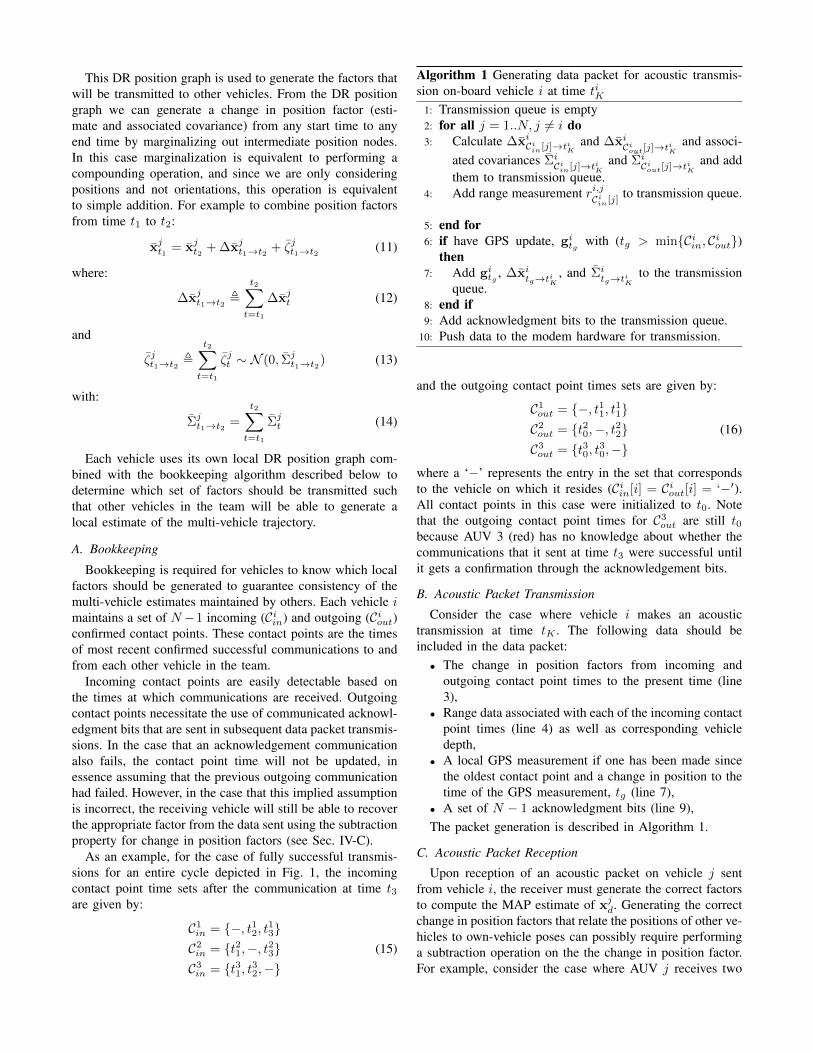
Algorithm 1 Generating data packet for acoustic transmis-sion on-board vehicle i at time tiK

1: Transmission queue is empty2: for all j = 1..N, j 6= i do3: Calculate ∆x̄iCiin[j]→tiK

and ∆x̄iCiout[j]→tiKand associ-

ated covariances Σ̄iCiin[j]→tiKand Σ̄iCiout[j]→tiK

and addthem to transmission queue.

4: Add range measurement ri,jCiin[j]to transmission queue.

5: end for6: if have GPS update, gitg with (tg > min{Ciin, Ciout})

then7: Add gitg , ∆x̄i

tg→tiK, and Σ̄i

tg→tiKto the transmission

queue.8: end if9: Add acknowledgment bits to the transmission queue.

10: Push data to the modem hardware for transmission.

and the outgoing contact point times sets are given by:

C1out = {−, t11, t11}C2out = {t20,−, t22}C3out = {t30, t30,−}

(16)

where a ‘−’ represents the entry in the set that correspondsto the vehicle on which it resides (Ciin[i] = Ciout[i] = ‘−′).All contact points in this case were initialized to t0. Notethat the outgoing contact point times for C3

out are still t0because AUV 3 (red) has no knowledge about whether thecommunications that it sent at time t3 were successful untilit gets a confirmation through the acknowledgement bits.

B. Acoustic Packet Transmission

Consider the case where vehicle i makes an acoustictransmission at time tK . The following data should beincluded in the data packet:• The change in position factors from incoming and

outgoing contact point times to the present time (line3),

• Range data associated with each of the incoming contactpoint times (line 4) as well as corresponding vehicledepth,

• A local GPS measurement if one has been made sincethe oldest contact point and a change in position to thetime of the GPS measurement, tg (line 7),

• A set of N − 1 acknowledgment bits (line 9),The packet generation is described in Algorithm 1.

C. Acoustic Packet Reception

Upon reception of an acoustic packet on vehicle j sentfrom vehicle i, the receiver must generate the correct factorsto compute the MAP estimate of xjd. Generating the correctchange in position factors that relate the positions of other ve-hicles to own-vehicle poses can possibly require performinga subtraction operation on the the change in position factor.For example, consider the case where AUV j receives two

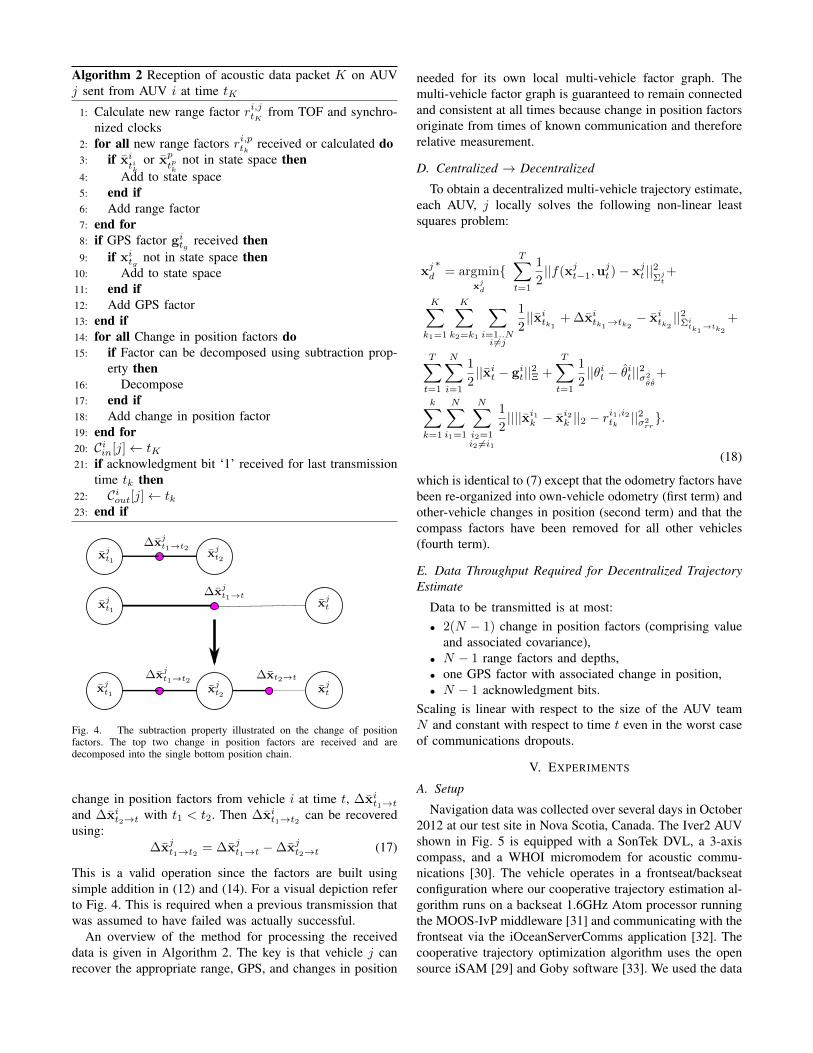
Algorithm 2 Reception of acoustic data packet K on AUVj sent from AUV i at time tK

1: Calculate new range factor ri,jtK from TOF and synchro-nized clocks

2: for all new range factors ri,ptk received or calculated do3: if x̄i

tikor x̄p

tpknot in state space then

4: Add to state space5: end if6: Add range factor7: end for8: if GPS factor gitg received then9: if xitg not in state space then

10: Add to state space11: end if12: Add GPS factor13: end if14: for all Change in position factors do15: if Factor can be decomposed using subtraction prop-

erty then16: Decompose17: end if18: Add change in position factor19: end for20: Ciin[j]← tK21: if acknowledgment bit ‘1’ received for last transmission

time tk then22: Ciout[j]← tk23: end if

x̄jt1

x̄jt

∆x̄jt1→t

∆x̄jt1→t2

∆x̄t2→t

x̄jt2

x̄jtx̄j

t1

x̄jt1

x̄jt2

∆x̄jt1→t2

Fig. 4. The subtraction property illustrated on the change of positionfactors. The top two change in position factors are received and aredecomposed into the single bottom position chain.

change in position factors from vehicle i at time t, ∆x̄it1→tand ∆x̄it2→t with t1 < t2. Then ∆x̄it1→t2 can be recoveredusing:

∆x̄jt1→t2 = ∆x̄jt1→t −∆x̄jt2→t (17)

This is a valid operation since the factors are built usingsimple addition in (12) and (14). For a visual depiction referto Fig. 4. This is required when a previous transmission thatwas assumed to have failed was actually successful.

An overview of the method for processing the receiveddata is given in Algorithm 2. The key is that vehicle j canrecover the appropriate range, GPS, and changes in position

needed for its own local multi-vehicle factor graph. Themulti-vehicle factor graph is guaranteed to remain connectedand consistent at all times because change in position factorsoriginate from times of known communication and thereforerelative measurement.

D. Centralized → Decentralized

To obtain a decentralized multi-vehicle trajectory estimate,each AUV, j locally solves the following non-linear leastsquares problem:

xjd∗

= argminxjd

{T∑t=1

1

2||f(xjt−1,u

jt )− xjt ||2Σjt+

K∑k1=1

K∑k2=k1

∑i=1..Ni6=j

1

2||x̄itk1 + ∆x̄itk1→tk2

− x̄itk2||2Σ̄itk1→tk2

+

T∑t=1

N∑i=1

1

2||x̄it − git||2Ξ +

T∑t=1

1

2||θit − θ̂it||2σ2

θ̂θ̂

+

k∑k=1

N∑i1=1

N∑i2=1i2 6=i1

1

2||||x̄i1k − x̄i2k ||2 − r

i1,i2tk||2σ2

rr}.

(18)

which is identical to (7) except that the odometry factors havebeen re-organized into own-vehicle odometry (first term) andother-vehicle changes in position (second term) and that thecompass factors have been removed for all other vehicles(fourth term).

E. Data Throughput Required for Decentralized TrajectoryEstimate

Data to be transmitted is at most:• 2(N − 1) change in position factors (comprising value

and associated covariance),• N − 1 range factors and depths,• one GPS factor with associated change in position,• N − 1 acknowledgment bits.

Scaling is linear with respect to the size of the AUV teamN and constant with respect to time t even in the worst caseof communications dropouts.

V. EXPERIMENTS

A. Setup

Navigation data was collected over several days in October2012 at our test site in Nova Scotia, Canada. The Iver2 AUVshown in Fig. 5 is equipped with a SonTek DVL, a 3-axiscompass, and a WHOI micromodem for acoustic commu-nications [30]. The vehicle operates in a frontseat/backseatconfiguration where our cooperative trajectory estimation al-gorithm runs on a backseat 1.6GHz Atom processor runningthe MOOS-IvP middleware [31] and communicating with thefrontseat via the iOceanServerComms application [32]. Thecooperative trajectory optimization algorithm uses the opensource iSAM [29] and Goby software [33]. We used the data

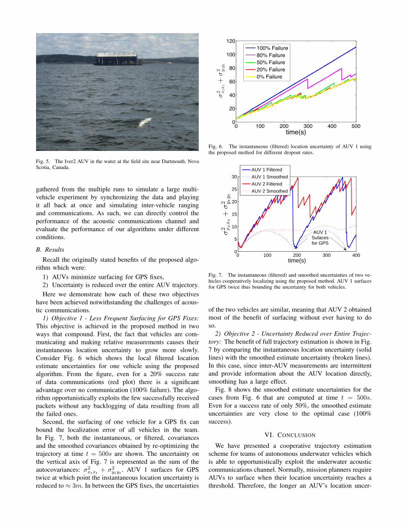
Fig. 5. The Iver2 AUV in the water at the field site near Dartmouth, NovaScotia, Canada.

gathered from the multiple runs to simulate a large multi-vehicle experiment by synchronizing the data and playingit all back at once and simulating inter-vehicle rangingand communications. As such, we can directly control theperformance of the acoustic communications channel andevaluate the performance of our algorithms under differentconditions.

B. Results

Recall the originally stated benefits of the proposed algo-rithm which were:

1) AUVs minimize surfacing for GPS fixes,2) Uncertainty is reduced over the entire AUV trajectory.Here we demonstrate how each of these two objectives

have been achieved notwithstanding the challenges of acous-tic communications.

1) Objective 1 - Less Frequent Surfacing for GPS Fixes:This objective is achieved in the proposed method in twoways that compound. First, the fact that vehicles are com-municating and making relative measurements causes theirinstantaneous location uncertainty to grow more slowly.Consider Fig. 6 which shows the local filtered locationestimate uncertainties for one vehicle using the proposedalgorithm. From the figure, even for a 20% success rateof data communications (red plot) there is a significantadvantage over no communication (100% failure). The algo-rithm opportunistically exploits the few successfully receivedpackets without any backlogging of data resulting from allthe failed ones.

Second, the surfacing of one vehicle for a GPS fix canbound the localization error of all vehicles in the team.In Fig. 7, both the instantaneous, or filtered, covariancesand the smoothed covariances obtained by re-optimizing thetrajectory at time t = 500s are shown. The uncertainty onthe vertical axis of Fig. 7 is represented as the sum of theautocovariances: σ2

xtxt + σ2ytyt . AUV 1 surfaces for GPS

twice at which point the instantaneous location uncertainty isreduced to ≈ 3m. In between the GPS fixes, the uncertainties

0 100 200 300 400 5000

20

40

60

80

100

120

time(s)

σ2 xtx

t+

σ2 yty

t

100% Failure80% Failure50% Failure20% Failure0% Failure

Fig. 6. The instantaneous (filtered) location uncertainty of AUV 1 usingthe proposed method for different dropout rates.

0 100 200 300 4000

5

10

15

20

25

30

time(s)

σ2 xtxt+

σ2 ytyt

AUV 1 Filtered

AUV 1 Smoothed

AUV 2 Filtered

AUV 2 Smoothed

AUV 1Sufacesfor GPS

Fig. 7. The instantaneous (filtered) and smoothed uncertainties of two ve-hicles cooperatively localizing using the proposed method. AUV 1 surfacesfor GPS twice thus bounding the uncertainty for both vehicles.

of the two vehicles are similar, meaning that AUV 2 obtainedmost of the benefit of surfacing without ever having to doso.

2) Objective 2 - Uncertainty Reduced over Entire Trajec-tory: The benefit of full trajectory estimation is shown in Fig.7 by comparing the instantaneous location uncertainty (solidlines) with the smoothed estimate uncertainty (broken lines).In this case, since inter-AUV measurements are intermittentand provide information about the AUV location directly,smoothing has a large effect.

Fig. 8 shows the smoothed estimate uncertainties for thecases from Fig. 6 that are computed at time t = 500s.Even for a success rate of only 50%, the smoothed estimateuncertainties are very close to the optimal case (100%success).

VI. CONCLUSION

We have presented a cooperative trajectory estimationscheme for teams of autonomous underwater vehicles whichis able to opportunistically exploit the underwater acousticcommunications channel. Normally, mission planners requireAUVs to surface when their location uncertainty reaches athreshold. Therefore, the longer an AUV’s location uncer-

0 100 200 300 400 5000

20

40

60

80

100

120

time(s)

σ2 xtxt+

σ2 ytyt

100% Failure80% Failure50% Failure20% Failure0% Failure

Fig. 8. The location uncertainty of the smoothed estimate at time t = 500sof AUV 1 using the proposed method for different dropout rates.

tainty is maintained below the threshold, the less frequentlyit needs to surface. In addition, gathered sensor data will bemore accurately localized through full trajectory estimation.

Future work in this direction includes a large multi-vehicle deployment and extension to the full cooperativesimultaneous localization and mapping scenario.

REFERENCES

[1] F. S. Hover, R. M. Eustice, A. Kim, B. Englot, H. Johannsson,M. Kaess, and J. J. Leonard, “Advanced perception, navigation andplanning for autonomous in-water ship hull inspection,” Int. J. ofRobotics Research, vol. 31, no. 12, pp. 1445–1464, 2012.

[2] C. Kaminski, T. Crees, J. Ferguson, A. Forrest, J. Williams, D. Hopkin,and G. Heard, “12 days under ice; an historic auv deployment inthe canadian high arctic,” in Autonomous Underwater Vehicles (AUV),2010 IEEE/OES, Sept 2010, pp. 1–11.

[3] L. Paull, S. Saeedi, M. Seto, and H. Li, “Sensor-driven online cov-erage planning for autonomous underwater vehicles,” Mechatronics,IEEE/ASME Transactions on, vol. 18, no. 6, pp. 1827–1838, Dec 2013.

[4] ——, “AUV navigation and localization: A review,” Oceanic Engi-neering, IEEE Journal of, vol. 39, no. 1, pp. 131–149, Jan. 2014.

[5] R. Kurazume, S. Nagata, and S. Hirose, “Cooperative positioning withmultiple robots,” in Robotics and Automation, 1994. Proceedings.,1994 IEEE International Conference on, May 1994, pp. 1250–1257.

[6] I. Rekleitis, G. Dudek, and E. Milios, “Multi-robot collaboration forrobust exploration,” in Robotics and Automation, IEEE InternationalConference on, vol. 4, 2000, pp. 3164–3169.

[7] S. I. Roumeliotis and I. M. Rekleitis, “Propagation of uncertaintyin cooperative multirobot localization: Analysis and experimentalresults,” Autonomous Robots, vol. 17, pp. 41–54, 2004.

[8] A. Mourikis and S. Roumeliotis, “Performance analysis of multirobotcooperative localization,” Robotics, IEEE Transactions on, vol. 22,no. 4, pp. 666–681, Aug. 2006.

[9] S. Roumeliotis and G. Bekey, “Distributed multirobot localization,”Robotics and Automation, IEEE Transactions on, vol. 18, no. 5, pp.781–795, Oct. 2002.

[10] M. Fallon, G. Papadopoulos, and J. Leonard, “A measurement distri-bution framework for cooperative navigation using multiple AUVs,” inRobotics and Automation (ICRA), 2010 IEEE International Conferenceon, May 2010, pp. 4256–4263.

[11] S. E. Webster, R. M. Eustice, H. Singh, and L. L. Whitcomb, “Ad-vances in single-beacon one-way-travel-time acoustic navigation forunderwater vehicles,” The International Journal of Robotics Research,vol. 31, no. 8, pp. 935–950, 2012.

[12] E. Nerurkar and S. Roumeliotis, “Asynchronous multi-centralizedcooperative localization,” in Intelligent Robots and Systems, Interna-tional Conference on, Oct. 2010, pp. 4352–4359.

[13] ——, “A communication-bandwidth-aware hybrid estimation frame-work for multi-robot cooperative localization,” in Intelligent Robotsand Systems, International Conference on, Nov 2013, pp. 1418–1425.

[14] E. D. Nerurkar, K. X. Zhou, and S. Roumeliotis, “A hybrid esti-mation framework for cooperative localization under communicationconstraints,” in Intelligent Robots and Systems (IROS), 2011 IEEE/RSJInternational Conference on, 2011, pp. 502–509.

[15] A. Cunningham, K. Wurm, W. Burgard, and F. Dellaert, “Fullydistributed scalable smoothing and mapping with robust multi-robotdata association,” in Robotics and Automation (ICRA), 2012 IEEEInternational Conference on, May 2012, pp. 1093–1100.

[16] J. M. Walls and R. M. Eustice, “An exact decentralized cooperativenavigation algorithm for acoustically networked underwater vehicleswith robustness to faulty communication: Theory and experiment,” inProceedings of the Robotics: Science & Systems Conference, Berlin,Germany, June 2013.

[17] L. Paull, M. Seto, and H. Li, “Area coverage that accounts for poseuncertainty with an AUV surveying application,” in IEEE InternationalConference on Robotics and Automation, 2014, pp. 6592–6599.

[18] A. Howard, M. Matark, and G. Sukhatme, “Localization for mobilerobot teams using maximum likelihood estimation,” in IntelligentRobots and Systems, 2002. IEEE/RSJ International Conference on,vol. 1, 2002, pp. 434–439.

[19] E. Nerurkar, S. Roumeliotis, and A. Martinelli, “Distributed maximuma posteriori estimation for multi-robot cooperative localization,” inRobotics and Automation, 2009. ICRA ’09. IEEE International Con-ference on, May 2009, pp. 1402–1409.

[20] A. Prorok and A. Martinoli, “A reciprocal sampling algorithm forlightweight distributed multi-robot localization,” in Intelligent Robotsand Systems, International Conference on, 2011, pp. 3241–3247.

[21] N. Trawny, S. Roumeliotis, and G. Giannakis, “Cooperative multi-robot localization under communication constraints,” in Robotics andAutomation, 2009. ICRA ’09. IEEE International Conference on, May2009, pp. 4394–4400.

[22] L. Carrillo-Arce, E. Nerurkar, J. Gordillo, and S. Roumeliotis, “De-centralized multi-robot cooperative localization using covariance in-tersection,” in Intelligent Robots and Systems (IROS), 2013 IEEE/RSJInternational Conference on, Nov 2013, pp. 1412–1417.

[23] K. Leung, T. Barfoot, and H. Liu, “Decentralized localization ofsparsely-communicating robot networks: A centralized-equivalent ap-proach,” Robotics, IEEE Transactions on, vol. 26, no. 1, pp. 62 –77,feb. 2010.

[24] A. Bahr, J. J. Leonard, and M. F. Fallon, “Cooperative localizationfor autonomous underwater vehicles,” The International Journal ofRobotics Research, vol. 28, no. 6, pp. 714–728, Jun. 2009.

[25] S. Webster, J. Walls, L. Whitcomb, and R. Eustice, “Decentralizedextended information filter for single-beacon cooperative acousticnavigation: Theory and experiments,” Robotics, IEEE Transactions on,vol. 29, no. 4, pp. 957–974, Aug 2013.

[26] A. Bahr, M. Walter, and J. Leonard, “Consistent cooperative localiza-tion,” in Robotics and Automation, 2009. ICRA ’09. IEEE InternationalConference on, May 2009, pp. 3415–3422.

[27] S. Singh, M. Grund, B. Bingham, R. Eustice, H. Singh, and L. Freitag,“Underwater acoustic navigation with the WHOI Micro-Modem,” inOCEANS 2006, Sep. 2006, pp. 1–4.

[28] F. Dellaert and M. Kaess, “Square root SAM: Simultaneous locationand mapping via square root information smoothing,” Int. J. ofRobotics Research, vol. 25, no. 12, pp. 1181–1203, 2006.

[29] M. Kaess, A. Ranganathan, and F. Dellaert, “iSAM: Incrementalsmoothing and mapping,” Robotics, IEEE Transactions on, vol. 24,no. 6, pp. 1365–1378, Dec. 2008.

[30] L. Freitag, M. Grund, S. Singh, J. Partan, P. Koski, and K. Ball,“The whoi micro-modem: an acoustic communications and navigationsystem for multiple platforms,” in OCEANS, 2005. Proceedings ofMTS/IEEE, vol. 2, Sep. 2005, pp. 1086–1092.

[31] M. Benjamin, P. Newman, H. Schmidt, and J. Leonard, “An overviewof MOOS-IvP and a brief users guide to the ivp helm autonomysoftware,” http:// dspace. mit. edu/ bitstream/ handle/ 1721.1/45569/MIT-CSAIL-TR-2009-028.pdf, June 2009.

[32] S. Sideleau, May 2010, http:// oceanai. mit. edu/ moos-ivp/ docs/ Guide To iOcean Server Comms.pdf.

[33] T. Schneider and H. Schmidt, “Model-based adaptive behavior frame-work for optimal acoustic communication and sensing by marinerobots,” Oceanic Engineering, IEEE Journal of, vol. 38, no. 3, pp.522–533, July 2013.