Debt on Credit Enhancements

Fang Chen, Yan Xu, Tong Yu∗

∗All authors are from the College of Business Administration, University of Rhode Island. Emails:fchen@mail.uri.edu, yan xu@mail.uri.edu, tongyu@uri.edu. All errors are our own. Comments arewelcome.

Debt on Credit Enhancements

Abstract

We examine the effect of credit enhancements (CEs) on investment and firm value.

A benefit of CEs is the reduction of financial constraints induced underinvestment

through liquidity pooling, on the other hand, a cost of CEs is the amplified overin-

vestment through the weakened monitoring role of debt. Using a sample of public

corporate debts with CEs from 1990 to 2009, we find a negative effect of credit en-

hancement on the stock return upon the bond offering announcements. It appears

that the cost of CE use dominates the benefit; CE use is negatively associated with

firm value and firms issuing debt with CEs underperform those without. Further evi-

dence suggests that better investment opportunities and more debt use help alleviate

the negative CE effect.

Key words: Credit Enhancements; Financial Constraint; Overinvestments; Underin-

vestments

1 Introduction

A key feature of internal capital markets is cross subsidization. That is, conglomerates

have the potential to put together resources within the corporate border. The out-

let of such resources is however under heated debate. Studies supporting the internal

capital market efficiency contend that a key advantage of an internal capital market is

that it shields investment projects from the information and incentive problems that

plague external finance (e.g., Alchian, 1969, Williamson, 1975, Gertner, Scharfstein,

and Stein, 1994, and Stein, 1997). Supportive to this argument, Khanna and Tice

(2001) show that internal capital allocation in diversified firms functions efficiently by

tying up capital to investment opportunities. A competing line of research, in con-

trast, argues that internal capital market can hinder investment efficiency. Scharfstein

and Stein (2000) and Rajan, Servaes, and Zingales (2000), among others, highlight

the effect of agency problems and power grabbing to generate inefficient cross subsi-

dization across projects.

In this study,we explore the efficiency of a special type of internal capital markets

with a sample of credit enhancements (CEs thereafter) firms. With an CE arrange-

ment, bond issuers acquire a guaranty from a third party to secure their payments

when bond issuers are at default. A salient fact about CE is that up to this day,

the lion’s share of CEs is conducted within the corporate border, either through the

guaranty of parents for subsidiaries or the guaranty of subsidiaries for their parents.

Therefore CE within conglomerate is an unambiguous operation conducted through

internal capital markets: one division’s assets are used as collateral to raise financ-

ing that is diverted to other divisions. Therefore if CE affects firm valuation, then

studying CE can further our understanding about the efficiency of internal capital

markets.

It is highly likely that use of CE will affect firm valuation. The cross subsidiza-

tion of the internal capital markets is clearly reflected by use of CE. By combining

the divisional cash flows into a smooth aggregate cash flow, firms can raise their debt

1

capacity and enjoy tax benefits (Hege and Ambrus-Lakatos, 2005). In the case of con-

glomerates, the parent pools the liquidity and channel the funds to subsidiaries with

worthy projects through an efficient internal capital market. With the internal guar-

anty arrangement, firms can considerably benefit from reduced financial constraints

and lower cost of external capital. In contrast, the direct cost associated with the use

of CE includes only the small cost of filing to SEC. The direct cost is out of propor-

tion relative to the potential benefit. However, measured in terms of par value, only

a small fraction of corporate bonds were issued with CEs. It may seem puzzling that

no more firms consider CEs.

We conjecture that there must exist some indirect costs related to procurement

of CEs, and it must potentially be associated with the existence of internal capital

market. Our research questions then become, first, as an internal capital market

arrangement, would CE impact firm value? If so in which way? Second, firms are

heterogeneous, and the differences in their firm characteristics may influence the im-

pact of internal capital allocation through CE on firm value. Does the impact of CE

on firm value differ across firms with different level of growth opportunities? Would

the impact of CE on firm value differ between firms with a high debt level and those

with a low debt level?

To better understand the nature of CE, we first investigate the determinants of

the use of credit enhancement with a probit analysis for the period from 1990 to 2009.

Our unique sample includes all CEs used by the public firms and the guarantors are all

subsidiaries. The results show that firms with limited debt capacity are more likely to

use CE for debt and the choice of CE use is irrelevant to growth opportunities. Next

we examine the short-term valuation of the CE bond issuance. The market model

cumulative abnormal stock return in (-30, +30) period is -3.17% and significant at

1% level. The results shows the CE use conveys a unfavorable information to the

stock market. The regression confirms the negative contribution of CE use to the

negative stock reaction. In a long-term, we find in the regression of the Tobin’s Q on

the CE use, the coefficient on CE dummy is -0.61 and significant at 1% level. This

2

finding is robust after controlling a set of firm-specific characteristics and correcting

the self-selection bias.

By documenting a negative valuation on internal capital allocation, we provide

a direct evidence on the inefficiency of an internal capital market operation. Our

evidence also implies a direct agency cost of managers, which may be exacerbated

by the unique feature of CE. Specifically, CE use shifts the incentive of monitoring

on managers from many debt holders to one or two credit enhancers. However, the

monitoring of subsidiaries on their parents perhaps is just weak and inefficient.

Next, in the subsample analysis, we specifically test whether the effect of CE

on firm value differs across firms with different growth opportunities. The rationale

is that for firms with greater growth opportunities, the benefit of expanded debt

capacity from CE use is more likely to manifest, while resource misallocation is more

likely the concern for CE users with lower growth opportunities. Our findings indeed

support the conjecture. The results show that for firms with relatively low growth

opportunities, CE has a significant negative effect on firm value. Specifically, in the

group of firms with lowest growth opportunities, the coefficient of the CE dummy

in the regression of Q is -2.47 and statistically significant. In comparison, for firms

with high growth opportunities, the coefficient of the CE dummy in the regression of

Q is not significant. Our finding supports the notion that the sensitivity of internal

allocation of resource to growth opportunities has impact on firm value (Peyer and

Shivdasani, 2001). It is also consistent with Billett and Mauer (2003) that the firms

with more efficient internal capital markets are more highly valued.

Moreover, in firms with high debt level, firm debt issuance capacity is more likely

to be constrained, justifying the adoption of CE. We find that, for firms with a

low debt level, the coefficient of the CE dummy in the regression of Q is -1.28 and

statistically significant. While for firms with a high debt level, CE has no significant

effect on Q. The extent of negative impact of CE appears to be lower in firms in

the high leverage group. This finding is interesting given CE arrangements that we

3

analyze are within the corporate border. Firms become more sensible in allocating

internal resources when they face higher leverage in this particular setting. Our

findings therefore are not consistent with the prediction in Hege and Ambrus-Lakatos

(2002) such that the pooling of financial resources in an internal capital market may

magnify financial distress situations. Our evidence is also in contrast with those

documented in Lins and Servaes (2000) which show that the conglomerate discount

is actually steeper in poorly developed emerging markets, and those in Claessens et

al. (1999b) which find that during the 1998 Asian financial crisis, the conglomerate

discount in the Asian markets rose.

Our paper clearly points out a link between the internal resource allocation and

conglomerate value reduction, and contributes to the large literature on internal cap-

ital market allocation inefficiency. So far, the literature has largely focused on the

direct allocation of internal capital among firms while not on the source of these

internal funds. Our study fills this void.

Our paper also contributes to the literature on CE. By investigating the relation-

ship between CE and firm valuation, this study explores the implications of corporate

financing in an important yet largely overlooked area. In all, our evidence documents

the significantly negative effect of CE on firm value and its sensitivity to growth op-

portunities and debt level. Credit risk and various instruments purposed to mitigate

credit risk indeed ignited the fire during the recent financial crisis. As a result, a

careful study on the relationship among CE and firm value would not only benefit us

by unveiling potential risks from using CE, but also shed light on the drivers for the

recent financial crisis.

The paper proceeds as follows. In Section 2, we introduce the background of CE.

In Section 3, we review the literature on internal capital market and the relation

between financial constraints, investment and firm value. Section 4 presents the data

and sample, followed by the analysis on the impact of CE on firm value on Section

5. Section 6 tests whether the relation between CE and firm value differs by growth

opportunities and debt levels. Section 7 concludes the paper.

4

2 Backgrounds on Credit Enhancements

A recent global survey shows that the majority of more than 1100 risk managers

consider credit risk as one of the most important risks (Bodnar et al, 2011). Seeing

CE as an effective way to reduce credit risk, a significant proportion of corporate

bonds are issued with credit enhancement (CE). The percentage of corporate bonds

with CE increased from 2% in 1990 to 26% in 2010 in terms of dollar value. Overall,

corporate bonds have been sold for $16,711 billion (par value) during the period of

1990 to 2010. Of bonds issued in the same period, 17% ($2,853 Billion), by dollar

value, were issued with CE. After 2000, SEC greatly reduces the filing cost for the

parent/subsidiary guarantee transaction.

CE is used to protect bond holders from defaults by providing the guarantee to

the payment of principal, premium (if any) and interest of the underlying bonds in

case of default of issuers. The focus of this study is the external credit enhance-

ment for corporate bonds. Traditionally corporate bonds use three major types of

external enhancements: guarantee, insurance and letter of credit (LOC) which takes

96%, 3% and 1% of the total credit enhancement respectively from 1990 to 2010. In

forms of guarantee, guarantors are diversified. They can be parent firms/subsidiaries.

For example, MGM Mirage used all its domestic subsidiaries as guarantors for its

$225,000,000 bonds issued in 2001. They can also be independent firms. For exam-

ple, Nestle SA provided guarantee on $150,000,000 bonds issued by EMC in 2005.

Among 1432 CE bonds by public-listed firms from 1990 to 2009, 1092 CE bonds were

guaranteed by subsidiaries.

The major form of CE is that subsidiaries provide guarantee on bonds issued by

parents. It accounts for about 70% of all CE used by public firms. With the guaranty

from the subsidiaries, debt holders of the parents have recourse to the subsidiaries

if the parents default. Otherwise,these debt holders can’t have recourse on the sub-

sidiaries. In such CE arrangement, debt normally will be unconditionally guaranteed

by the guarantor.

5

Credit ratings is an important factor in the requirement by several regulations

on financial institutions’ and other intermediaries’ investments in bonds. For exam-

ple, regulations restrict banks from investment in speculative-grade bonds since 1936

(Partnoy, 1999; West, 1973). In 1989, savings and loans were required to completely

liquidate their speculative-grade bonds by 1994 (Kisgen, 2006). Finally, pension fund

guidelines often prevent bond investments from speculative-grade bonds (Boot, Mil-

bourn, and Schmeits, 2003). In order to attract financial institutional investors and

other intermediaries, debt borrowers use CE to increase credit rating of debt before

issuing. Should debt borrowers default, debt holders have recourse to guarantors.

Once a bond obtains credit enhancement, the rating agency will assign two ratings:

one is the rating for the underlining bond without the consideration of CE, another

one is the rating of the guarantor/insurer. The rating agency then gives the higher of

either one to the bond with CE. If the guarantor or insurer is downgraded, the rating

agency will reevaluate the bond and adjust the rating if needed. Since the guarantor

or insurer has the possibility of failing to fulfill its obligation of paying debt in case

of the default of the bond issuer, the credit risk for bonds with CE is reduced to the

least extent but not completely eliminated.

3 Literature Review and Hypotheses Development

3.1 Debate on Internal Capital Market Efficiency

Is the internal capital market efficient than external capital market? The debate on

the issue has been fierce. In the camp supporting internal capital market efficiency,

Williamson (1975) argues that the internal capital market of diversified firms might

allocate capital more efficiently than the external capital market because top man-

agement of a diversified firm knows more about the firm’s investment opportunities

than external investors. Further, Gertner, Scharfstein and Stein (1994) and Stein

6

(1997) propose models to identify the conditions for more efficient investment deci-

sions. These modes are mainly related to investment comparison between two forms of

organization: diversified firms and stand-alone firms. Specifically, Stein (1997) argues

that managers will be unwilling to cut investment when they have poor investment

opportunities. However, an internal capital market of diversified firms gives managers

a way to redeploy capital from divisions with poor investment opportunities to those

with good investment opportunities without compromising the overall capital budget.

Khanna and Tice (2001) examine capital expenditure decision of diversified firms in

response to WalMart’s entry to their market. They find diversified firms make quicker

decision of “exit” or “stay” and their capital expenditures are more sensitive to the

their productivity than focus firms. Hence, internal capital allocation in diversified

firms functions efficiently by tying up capital to investment opportunities.

Converse, a competing line of studies argue that internal capital market is in-

efficient. One important measure of capital allocation inefficiency is defined as di-

visions’ investment being independent on their investment opportunities. Lamont

(1997) shows that when oil prices are high, the non-oil divisions of diversified oil

producers increase their investment more than their industry counterparts and these

investments are inconsistent with their own investment opportunities. Shin and Stulz

(1998) find evidence that investment of small divisions of conglomerates depends on

cash flows of other divisions, not their own Q. Rajan, Servaes, and Zingales (2000)

show that when divisions have similar level of resources and opportunities, internal

fund allocation has a positive relation with their opportunities; when divisions have

diversified level of resources and opportunities, the relation between internal fund

allocation and opportunities turns into a negative one in which divisions with good

opportunities are ”poached” by other divisions. The inefficient capital allocation has

also been investigated by comparing the investment efficiency before and after spin-

off. Gertner, Powers, and Scharfstein (2002) examine spin-off divisions of diversified

conglomerates and find their investment becomes more sensitive to industry Q. Ahn

and Denis (2004) further find that for diversified firms after spin-off there is a signifi-

7

cant increase in measures of investment efficiency and firm value. They thus conclude

that internal capital allocation in diversified firms is inefficient.

Most of these studies compare conglomerate firms to their standalone counter-

parts and hence is subject to the criticisms of measurement errors (Whited, 2001;

Villalonga, 2000) and sample selection issues (Campa and Kedia, 2002; Chevalier,

2004). Another limitation also exists in the use of an industry Tobin’s Q as proxy

for growth opportunities which implicitly assume all firms, conglomerates and single-

segment firms have similar investment opportunities within an industry (Marksimovic

and Philips, 2002).

The conditions leading to an inefficient internal market have been investigated by

many researchers. Agency problem of division managers is regarded as one of the main

reasons for inefficient internal capital market efficiency. Scharfstein and Stein (2000)

argue that rent-seeking behavior of division managers will raise their bargaining power

and influence CEO to overinvest in the divisions with bad investment opportunities

and underinvestment in the divisions with good investment opportunities. Datta et al

(2009) suggest that CEO compensation makes difference in internal capital allocation.

Specifically, stock option is more effective than stock grant in reducing agency problem

and being incentive mechanism for efficient allocation. Ozbas and Scharfstein (2010)

find that in unrelated segments of diversified firms investment is less sensitivity than

stand-alone firms. Moreover, the ownership stakes of top management has a positive

relation with the extent of Q-sensitivity differences, suggesting that agency problem

leads to the inefficient capital market.

A key assumption in many studies is that division managers, especially in low-

growth divisions, are empire builder and rent-seekers while parents or CEOs act in

the maximum interest of firms. Mathew and Robinson (2008) base their model on

the assumption of the rational and profit-maximizing behavior on the part of parents.

Kolasinski (2009) builds his hypothesis on the assumption that the CEO would prefer

to commit ex ante to invest more in the high-growth division. Stein (1997) points

8

out that the control right of parents is the key for parents to move funds from less

desirable investments to more desirable ones. It implies that parent firms have to act

in the best interest of firms to make internal capital market efficient. However, the

fact that parents themselves are agents of investors raises the concern if they can act

in the maximum interest of firms. Bolton and Scrafstein (1998) point out because

allocating capital to divisions with opportunities aligns with parents’ empire-building

preference, it is not obvious that agency problem of parents leads to inefficient internal

capital allocation among divisions. Scharfstein and Stein (2000) argue that a two-tier

agency problem, stemming from misaligned incentives at parents and at divisions, is

necessary for ”corporate socialism” in internal capital allocation. Parents use their

authorities to have their bonds guaranteed by subsidiaries and such allocation may

be a consequence of empire-building preference of parents rather than following the

investment opportunities. The CE in the sample of this study is through subsidiary-

guarantee. We therefore postulate the following hypothesis:

H1. Credit enhancement has a negative effect on firm value.

3.2 Financial Constraints, Investments and Firm Value

Whited (1992) includes financial constraints into firms’ investment analysis and finds

firms’ ability to borrow money can explain the different investment patterns very

well. The implication of this finding is that borrowing constraints can lead to under-

investment, subsequently reduce firm value. Billett and Mauer (1994) document that

internal subsidies to small segments with financial constraints and relatively poor in-

vestment opportunities can increase the excess value of the segments. They conclude

that financial constraints affect the relationship between internal capital market and

firm value. A global survey of 1,050 Chief Financial Officers (CFOs) finds that the

majority of firms had to forgo attractive investment opportunities because of financial

constraints in the financial crisis of 2008 (Campello et al, 2010). CE can increase the

ratings of bonds and lessen firms’ financial constraints, thus leading to increased firm

9

value.

Growth opportunity is an important factor in influencing debt level and firm

value. For example, Vogt (1994) finds overinvestment in US manufacturing firms is

the strongest in the large, low-dividend firms with low Tobin’s Q. Lang, Ofek and Stulz

(1994) divide the firms into the high and low growth opportunities group and found

that only in the group with low growth opportunities leverage is negatively related

to subsequent growth of employees number and capital expenditure. McConnell and

Servaes (1995) empirically investigate the relation between leverage and firm value,

and find that this relation is impacted by growth opportunities. Specifically, firm

value is negatively correlated to leverage for the high-growth firms and is positively

correlated to the leverage for the low-growth firms. CE is in nature an internal capital

market allocation and thus it is better if parents have more favorable investment

opportunities. The fewer the growth opportunities, the more likely investment will

go to unprofitable projects. Moreover, the fewer the growth opportunities for a firm,

the less the benefit the firm would receive from reducing financial constraints. This

reasoning leads to the following empirical hypothesis:

H2. The higher growth opportunities of a bond issuer, the less negative effect of

credit enhancement on its firm value is.

Firm value is positively related to debt level since debt has a positive effect in pre-

venting overinvestment. Jensen (1986) argues that debt can reduce managers’ interest

in overinvestment due to the obligation of paying debt. Because of the separation of

corporate equity ownership and management, managers intend to reward themselves

by increasing the size of the firm beyond the optimal level for the shareholders. One

explanation is that managers consider the firm a source of self-esteem and a means

to increase their own human capital (Zingales, 1998). Once firms borrow debt, man-

agers will have to limit their investment on unprofitable projects to avoid bankruptcy.

Therefore, debt plays a monitoring role in reducing agency problem. D’Mello and Mi-

10

randa (2010) investigate the monitoring role of debt and find the new debt offering

by unlevered firms leads to a reduction in abnormal capital expenditure in firms with

overinvestment in real assets. As discussed before, CE weakens the monitoring of

debts. When parents have high level of non-CE bonds, the strengthened monitoring

from non-CE bondholders can mitigate weakening effect from CE to some extent.

Thus, we state the following hypothesis:

H3. The higher level of non-CE bonds of a bond issuer, the stronger monitoring

it has and the less negative effect CE on its firm value.

4 Data

We start with Mergent Fixed Income Securities Database (FISD) data for this study.

From 1990 to 2009, there are 101,428 corporate bonds issued by 7,110 firms† which

include 13,455 bonds issued by 2,428 public firms. Among all these corporate bond

issues, there are 11,765 third-party guarantee credit enhancement used by 1,273 firms

, including 1,422 third-party guarantee credit enhancements by 690 public firms.

Further, for each credit enhancement, We identify the relationship of issuer and guar-

antor from the guarantor description in FISD. If there is still unknown relationship,

We manually identify the guarantors from the prospectus or 10-k and then check the

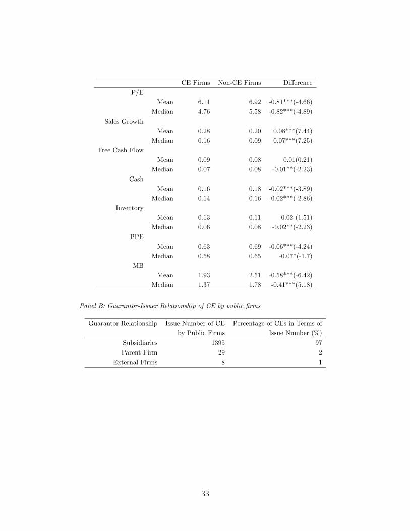
relationship from the Mergent online. Among all credit enhancements, 1395 (97%)

guarantors were subsidiaries, 29 (2%) guarantors were parent firms, 8 (1%) guarantors

were external firms. Since the majority of the guarantors in FISD credit enhancement

data were subsidiaries and the paper focus on the subsidiary-guarantee debt, all credit

enhancements which are not guaranteed by subsidiaries are excluded. The stock in-

formation for this sample is obtained from the Center for Research in Security Prices

(CRSP) and the financial data and the ratings are from COMPUSTAT. Following the

convention on bond research, we exclude the financial firms (SIC codes 6000-6999)

†The US corporate bonds include US corporate debt, US corporate MTN, asset-backed security

and other US corporate bonds but exclude the US corporate convertible, preferred stock.

11

and regulated utilities firms (SIC codes 4900-4999) from the sample. We also exclude

the firms missing sufficient data to compute valid Tobin’s Q.The final sample consists

of 8237 bonds issues by 1,657 public firms, including 1198 credit enhancements bonds

by 553 public firms.

In the short-term, the bond issuers are evaluated by their market model abnormal

return. In the long-term, the bond issuers are evaluated by their Tobin’s Q. Tobin’s Q

is computed as (total asset - book value of equity + market value of equity)/total asset.

Because all the bonds with credit enhancement are long-term bonds, we choose the

average S&P Domestic Long Term Issuer Credit Rating in the 12 months before the

offering date from COMPUSTAT . To reduce the effect of possible spurious outliers,

we winsorize the top and bottom 1 percentile of observations.

For the proxy for the growth opportunity, we follow the method of McConnell and

Servaes (1995) by using a firm’s price-to-operating-earnings (P/E) ratio. The ratio is

computed as stock price divided by the operating earnings per share at the end of the

corresponding year. Sales growth is used as a second proxy for growth opportunities

and is calculated as the average sales growth percentage in the last two years.

Descriptive statistics for bond-issuing firms with credit enhancement and those

without credit enhancement are presented in Table 2. The data period is in the year

before the debt offering. The differences in the firm characteristics between the CE

firms sample and the non-CE firms sample are dramatic. For example, Tobin’s Q for

two groups is significantly different. Mean (median) Tobin’s Q of the CE firms is 1.42

(1.22) and this value increases to 1.66 (1.35) for the non-CE firms. The results show

that the firms with CE have a lower market to book than those without CE. Two

proxies of growth opportunities, P/E and sales growth, have a different result in two

samples. the mean and median P/E of the CE firms are significantly lower than those

of non-CE firms. In contrast, sales growth for CE firms is significantly higher for the

CE firms that for the non-CE firms. The implication of this difference is that P/E

and sales growth may capture a different aspect of growth opportunities. Considering

12

this possibility, we estimate the regression for the high growth and the low growth

samples using P/E and sales growth respectively. The S&P long-term domestic debt

rating for CE firms is lower than that for non-CE firms.

As shown by Table 2, bond-issuing firms with credit enhancement tend to have a

higher debt level, smaller size, lower ROA, lower market-to-book, lower P/E, less free

cash flow, lower long-term credit rating by S&P, higher sales growth than those with-

out credit enhancement. Except free cash flow and inventory, all the mean differences

are statistically significant.

5 Analysis of the Use and the Valuation Effect of

Credit Enhancements

5.1 Probit Analysis on the Use of Credit Enhancement

The first step is to use probit regression to examine the determinants of CE use (Y).

A bond issuer either takes CE (Y=1) or doesn’t (Y=0) in the sample. A set of factors

in a vector x explains the decision. We model the probability that an insurer uses

CE as a probit function:

Pr(Y ∗) = Φ(β′X) (1)

where Y* is not observable while we can observe y, Φ(.)denotes the standard normal

distribution, X is a set of variables explaining bond issuers’ propensity to use CE

(discussed below). The set of parameters β′ reflects the impact of changes in on the

probability.

In the setting of probit, we have:

Y = 1 when Y ∗ > 0 (2)

Y = 0 when Y ∗ <= 0 (3)

13

The potential economic benefit of new debt is the motivation of debt issuers. The

bond yield in the markets and the firm’s growth opportunities are used to control for

the benefit. We use the average annual yield of Moody’s AAA and Baa bonds.The

lower the yield of bonds in the market, the more likely the firms issue new debt to

retire the old debt or invest in new projects. P/E ratio and sales growth are used as

the proxies for growth opportunities. When a firm has higher growth opportunities,

the benefit from raising capital from debt is more likely to manifest.

Another potential benefit of debt is to reduce the agency problem from free cash

flow. Jenson (1986) argues that a firm with high free cash flows should issue debt to

prevent managers from wasting it. However, a firm with free cash may not be able

to issue debt if it has financial constraints. With the credit enhancement, the firm

can extend its debt capacity and mitigate the agency problem. We expect a positive

relationship between the free cash flow and the use of credit enhancement.

The firms with financial constraints are in greater need of CEs than firms without

financial constraints to extend their debt capacity. The proxies for debt capacity

vary in previous researches. Rating controls for a firm’s default risk which is directly

related to the firm’s debt capacity. The lower the credit rating, the higher the default

risk a firm has and the more difficult for the firm to issue bonds. Therefore firms with

lower credit rating are expected to be more likely to use CEs. Size affects the firms’

ability to issue debt (Whited, 1992). Small firms have more information asymmetry

than larger firms and lack collateral to back up their borrowing. Consequently, small

firms have limit access to debt market. Dividend payout by a firm shows its debt

capacity. A firm that doesn’t pay dividends is regarded as a firm with difficulty

for external capital (Fazzari, 1988). Collateral indicates a firm’s payback ability in

case of default. Bernanke and Campbell (1988) advocate that three variables can be

used to measure a firm’s collateral for external capital. These three variables are cash,

inventory, PPE(property, plant and equipment). Debt has the negative impact on the

debt capacity. On one hand, high debt level indicates a high level of default risk. On

the other hand, the over-hang problem arising from existing debt prevents firms from

14

issuing new debt (Myers, 1977; Hart and Moore, 1989; Hart ,1991). The profitability

is also a typical proxy for debt capacity in the corporate finance literature.

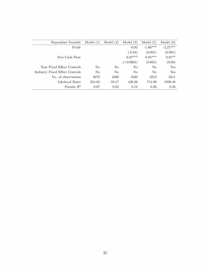
To control for time-varying macroeconomic factors, we include the year-fixed ef-

fects in the last specification. Accordingly, to control the industry specific factors, we

include the two-digit sic fix-industry effects in the last specification.

Table 3 reports the result of the probit regression. Except the coefficient on

inventory, the coefficients on the variables proxy for a firm’s debt capacity are all

significant at 1% level. Specifically, credit rating, size, dividend payout dummy, cash,

PPE, profit and debt are significantly negatively related to the choice of CE use. The

result shows the extending debt capacity is a main determinant of CE use.

The coefficient on free cash flow is positive and significant at 5% level. It is

consistent with the postulation that the firms with financial constraints are more

likely than the firms without financial constraints to use CE to mitigate the agency

problem from free cash flow.

The coefficient on the bond yield in the market is significantly negative. But after

including the fixed-year and fix-industry effect, the coefficient is not significant. Both

proxies of growth opportunities have no significant positive impact on the choice of CE

use. The coefficient on P/E ratio is -0.03 and significant at 1% level. The coefficient

on sales growth is no significant in the last three models. The result implies that the

potential economic benefit, both low bond yield and high growth opportunities, are

irrelevant to the choice of CE use.

last, we fail to find evidence that firms with high inventory are less likely to use

CE.

5.2 Short-term Valuation Effect of Credit Enhancements

The use of CE on bonds conveys information of the bond issuers to the market. The

stock price response to the initial announcement of a new debt issuance reflects the

15

investors’ interpretation of the information. The new debt issuance increases the

leverage whose sign of change is positively related to the sign of stock price change.

For example, the stock repurchase [Masulis (1980), Dann (1981), Vermaelen (1981)]

has a positive two-day announcement period stock return; while convertible debt

calls [Mikkelson (1981)] and common stock issuance [Korwar (1982), Asquith and

Mullins (1983)] have a negative two-day announcement period stock return. One

explanation is the information signalling model of Ross (1977). In this model, the

increase of leverage conveys favorable information and the decrease of leverage conveys

unfavorable information.

CE on debt not only conveys the leverage increase information but also reflects

more information of the firm. The main information of the firm is revealed by the

use of CE in two ways. First, the parent firm itself has limited debt capacity which

may raise from its high default risk. Second, by the new debt guaranteed by its

subsidiaries, the parent firm allocates the internal capital. The inefficiency of internal

capital market allocation has been well identified by previous research. Therefore the

price response to the announcement of a CE debt offering is a net effect of the positive

information from increasing leverage and the negative information from high default

risk and potential inefficient internal market.

Panel A of table 4 presents a time series of average daily market-model common

stock abnormal return centered around the announcement dates (day 0). Column

(2) indicates the slight significantly negative abnormal return between trading days

-10 and +10 for CE bonds. While column (5) shows no significant abnormal return

during the same period for non-CE bonds.

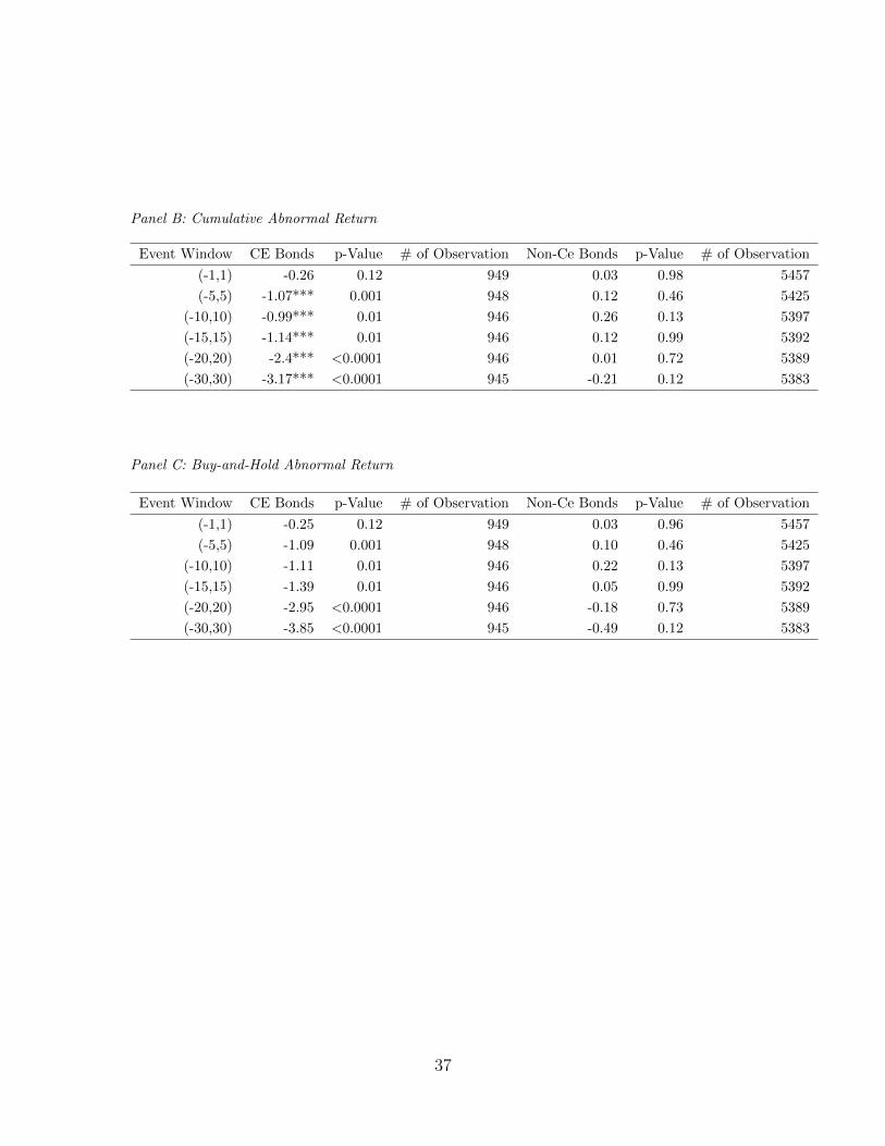
Panel B of table 4 reports the cumulative abnormal return (CAR) and panel C

of table 4 reports the buy-and-hold abnormal return. In both panels, the stock price

reaction is significantly negative to the CE bond offerings and no significant to the

non-CE bond offerings. Specifically, CAR in (-5,+5) period for CE bonds offering

is -1.07% and significant at 1% level. Considering the possible information leakage,

16

CAR in (-30, +30) period has a stronger stock price reaction which is -3.17% and

significant at 1% level. Buy-and-hold abnormal return in (-5,+5) period for CE bonds

offering is -1.09% and significant at 1% level. Additionally, Buy-and-hold abnormal

return in (-30,+30) period for CE bonds offering is -3.85% and significant at 1% level.

The result the market interprets the use of CE as a unfavorable information overall.

To further quantify the contribution of CE use to the negative stock price reac-

tion, we use a regression. CAR is the dependable variable of the regression. The

independent variables include a CE dummy variable for CE use, a set of bonds char-

acteristics like maturity, offering amount, callable dummy, putable dummy and con-

versable dummy, and a set of firms factors like size, profitability and debt. We use

the fixed-year control variable to control the macro economic effect and fixed-industry

variable to control the industry effect.

The result of the regression is reported in table 5. In all models of the regression,

credit enhancement use lowers the abnormal return and the effect is statistically

significant. In model 1, the coefficient on CE dummy is -0.03 and significant at

1% level. In model 2, we add the fix-year and fix-industry effect. The coefficient

on CE dummy is -0.04 and significant at 1% level. In model 3, we add the bonds

characteristics and in model 4, we add the firms factors. The coefficient on CE

dummy remains unchanged at -0.03. In model 5, we add all above variables into the

regression and the coefficient on CE dummy is -0.03 and significant. In other words,

the negative effect of credit enhancement use on stock price reaction is robust after

controlling the bonds characteristics and firm factors.

5.3 Long-term Valuation Effect of Credit Enhancements

The next step of the analysis is to investigate the effect of CE on firm value. We

estimate a regression of the Tobin’s Q of the firms on CE dummy variable and a set

of control variables. A number of firm characteristics serve as control variables in the

regression.

17

• CE is a dummy variable for the use of credit enhancement. It takes a value of

1 for a CE firm and 0 for a non-CE firm.

• P/E ratio is the proxy for the growth opportunities. It has been shown to have

impact on the relationship between firm value and debt level (McConnell and

Servaes, 1995).

• Sales Growth is another proxy for growth opportunities (McConnell and Ser-

vaes,1995; Doidge et al 2004).

• Free Cash Flow is a proxy for overinvestment probability. In Jenson (1986),

firms with free cash flow and low growth opportunities are more likely to have

overinvestment problem when managers have empire-building preference.

• Debt has impact on investment and default risk. On one hand, high debt level

induces underinvestment and reduces overinvestment. On the other hand, high

debt level indicates a financial distress risk and may lower the firm value.

• ROA is related to the firm value directly.

• Size is total asset. Small firms are well known to outperform large firms.

• Rating is used to measure the benefit of CE use. The lower the firm rating is,

the more benefit it receives from CE. Therefore rating has an effect on the firm

value.

In addition, fixed Year Effect is used to capture the impact of time-varying macroe-

conomic factors.

It is worth noting that firms with lower Q are more likely to use CE than those

with higher Q. With this self-selection, the error in the regression is therefore likely

to be correlated to a firm’s decision to whether use CE or not. This correlation will

create a selection bias in the estimate of the coefficient of the CE dummy variable in

the valuation regression. The econometric problem we face is similar to the treatment

18

effects in Heckman model, therefore we also use Heckman’s (1979) two-step estimator.

To examine the effect of CE, we use a valuation regression of Q as:

Qi = α + β′Xi + δCEi + εi (valuation equation) (4)

where Xi is a set of exogenous variables, CEi is a dummy variable that equals one for

a firms that use CE for bond issuing. α, β, δ is a vector of parameters to be estimated

and εi is an error term. δ measure the relation between CEi and Qi. If a firm’s

decision to use CE is related to Q, CEi and εi are correlated and the estimate of δ

will be biased.

To correct the bias, according to Heckman (1979), a reduced form CE decision

equation is given by:

CE∗i = γ′Zi + ν (CE decision equation) (5)

where CE∗i is an unobserved latent variable. We observe only an indicator variable

for the CE decision, defined as CEi = 1 if CE∗i > 0 and CEi = 0 if CE∗i <= 0. Zi is a

set of variables that affects the decision to use CE and µ is an error term. In addition

to the basic structure, the Heckman model requires the following assumption:

(1)µ =

(µε

µν

), σ =

(σ2ε ρσεσnu

ρσεσnu σ2ν

), bivariate normal distribution;

(2)(ε, ν) is independent of X and Z;

(3)var(ν) ≡ σ2ν ≡ 1;

Then the expected Q of the CE firm can be expressed as:

E((Qi| = CEi) = 1) = α + β′Xi + δ + ρσελi,1(γ

′Zi) (6)

Where λi,1(γZi is the ”inverse Mills’ ratio” (IMR) and is estimated as φ(γ′/Φ(γ′Zi),

where φ(.) and Φ(.) are the density function and cumulative standard normal distri-

bution functions respectively. Similarly, we have the expected Q of the non-CE firm

as:

E((Qi| = CEi) = 0) = α + β′Xi + δ + ρσελi,2(γ

′Zi) (7)

19

Where λi,2 is estimated as −φ(γ′Zi)/Φ(γ′Zi)(1 − Φ(γ′Zi)) . The difference of Q for

CE firm and non-CE firms is computed as:

E((Qi| = CEi) = 1)− E((Qi| = CEi) = 0) = δ + ρσεφ(γ′Zi)/[Φ(γ

′Zi)(1− Φ(γ

′Zi)] (8)

From equation (8), if low Q firms tend to choose CE, the low Q after use of CE is

positively related to the low Q before use of CE. Such the correlation of the error

terms, ρ , between two equations are positive and the bias of valuation on CE firms

is upwards.

The first step in Heckman (1979) model is to run a probit model of using CE

for all the firms. The estimates of the γ from this probit model are then used to

computed the ”inverse Mills’ ratio” (IMR, denoted as lambda in the below). In the

second step, the valuation equation now becomes:

Qi = α + β′Xi + δCEi + θLambdai + ei (9)

Where the θi captures the sign of correlation between the error terms in both equation.

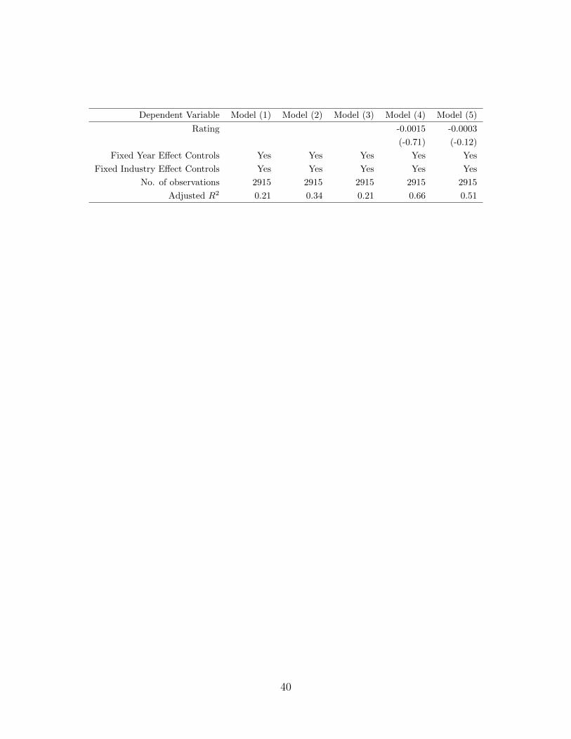
The result of Heckman model is reported in Table 6. Specifications (1) to (5)

are the results for regressions of Q on the CE choice and a set of control variables

after controlling for the self-selection bias. Lambda, inverse Millers’ ratio (IMR) in

Heckman’s model, is significantly positive at all regressions and it shows the error

term in the selection regression and the valuation regression are positively related.

The result confirms the previous finding that low Q firms are more likely to choose

CE. After introducing the selection correction variable Lambda in the regression, the

explanatory power of CE dummy variable becomes economically stronger and stays

statistically significant.

In Specification (1), the CE dummy variable has a coefficient of -1.18 with a

t-statistic of -12.67. One may argue this negative effect of CE on bonds is due

to the fact that firms with CE has less growth opportunities and thus lower firm

value. In specification (2) and (3), we use two proxies for growth opportunities:

20

P/E ratio and sales growth. The results show the coefficient of the dummy variable

CE is still significantly negative even after controlling for the growth opportunities.

Controlling for growth opportunities reduces the magnitude of negative effect from

CE only slightly.

In specification (4) and (5), we add other firm variables. The coefficient of the

dummy variable CE is significant in both regressions. These overall results are con-

sistent with the conjecture and suggest that CE has a significant negative impact on

firm value. In the last specification (4), the regression includes the control variables

CE dummy, P/E, free cash flow, sale growth, debt, ROA, size, and rating. The co-

efficient of CE dummy is -0.61 with a t-statistic -5.84 and R2= 0.51. Except for the

rating, all other variables are significant. In particular, bond issuing firms with lower

free cash flow, higher debt level and higher ROA have higher Q. Bond issuing firms

with low rating (high rating number), large size, short firm history tend to have lower

Q. In sum, the negative effect of CE on firm value is robust after controlling for a set

of a firm’s financial characteristics and self-selection bias.

6 Valuation Effect of Credit Enhancement for Dif-

ferent Subsamples

This section investigates whether the impact of CE on firm value differs between firms

with high growth opportunities and those with low growth opportunities, and differs

between firms with a high debt level and a low debt level.

6.1 Valuation Effect of Credit Enhancement for Firms with

Different Growth Opportunities

For growth opportunities, we first divide the sample into five groups based on their

P/E ratio in the year of the bond issuing. To quantify the impact of growth oppor-

21

tunities, we estimate two regressions with the same set of control variables on the

highest P/E (growth opportunities) group and the lowest P/E (growth opportuni-

ties) group respectively. The regressions include a dummy variable CE that takes the

value of one if it uses CE and zero otherwise. Comparing the coefficients CE dummy

variable in the regression of the high P/E dummy variable and the low P/E dummy

variable reveals the effect of P/E (growth opportunities) on the relationship between

CE use and firm value.

Table 7 reports the results of the regressions. In the lowest P/E (growth oppor-

tunities) group, coefficient for CE is -2.47 (t=-2.83) while that for the highest P/E

(growth opportunities) group is -0.15(t=-0.19). It can be seen that the reduction in

Q from CE in the lowest grow opportunities group is 2.32 higher than that in the

highest grow opportunities group. The magnitude of the coefficient of CE in the low-

est growth opportunities group indicates that the negative effect of CE on firm value

is economically significant when firms lack growth opportunities. Comparing the co-

efficient of CE in the lowest growth opportunities quintile with that in the highest

growth opportunities quintile, one can see that the impact of CE on firm value is

affected negatively by growth opportunities.

The empirical results may depend on the proxy of growth opportunities. As an

alternative measure of growth opportunities, we used sales growth. Again, we divide

the sample into five groups based on the sales growth in the year of bond issuing and

perform one additional sensitivity test on the sales growth. The regression result is

reported in Table 8. Similar to Table 7, there is a significant negative effect of CE on

firm value in the lowest sales growth (growth opportunities) group and no significant

effect of CE on firm value is found in the highest sales growth (growth opportunities)

group. The result further confirms the conjecture that the impact of CE on firm value

has a negative relation with growth opportunities.

The finding supports the view that the internal capital allocation is inefficient

(Scharfstein and Stein, 2000; Rajan, Servaes, and Zingales, 2000). The inefficiency

22

stems from the fact that capital flows to the divisions or subsidiaries with few growth

opportunities. In firms with few growth opportunities, the benefit of expanded debt

capacity from CE use is small and overinvestment is more likely. The cost of CE is

more likely to dominate the benefit of CE. Therefore the negative effect of CE on

firm value is more pronounced in firms with few opportunities.

6.2 Valuation Effect of Credit Enhancement for Firms with

Different Leverage

Next, we break down firms into different leverage groups. To check the impact of debt

level, we divide the sample into five groups based on their debt ratio in the year of the

bond issuing. We then estimate two regressions with the same set of control variables

on the highest debt group and the lowest debt group respectively. The regressions

also include a dummy variable CE.

Table 9 reports the results of the regressions. In the lowest debt group, coefficient

for CE is -1.28 (t=-1.83). In contrast, in the highest debt group coefficient of CE

is -0.66(t=-0.70), which only equals to half of the value in the other group. The

result supports the conjecture that firms with a high debt level is less sensitive to

the negative effect of CE. The benefit of CE on firms with high debt is two-fold.

First, there is reduction on high constraints of debt capacity. Secondly, the strong

monitoring of non-CE debt holders achieves in weakening agency problem, which is

the culprit for the inefficient internal capital market allocation.

In sum, the growth opportunities and debt level have impact on the effect of CE

on firm value and the internal capital allocation efficiency.

23

7 Conclusions

In an increasing trend, firms allocate their internal capital by internal sponsored

guarantee on their debt. This study explores the impact of CE on firm value and

whether the relationship between CE and firm value differs by growth opportunities

and debt levels. CE may affect firm value both positively and negatively. The positive

effect of CE on firm value stems from lessening financial constraints and reducing the

default risk of debt. The negative effect of CE is caused by weakened monitoring

on agency problem, a well identified reason for inefficient internal capital market

allocation (Scraftstein and Stein, 2000). We find a significant negative stock market

reaction on the announcement day of debt offering with CEs. Further, the results of

this empirical test show that bond issuing firms with CE have a significantly lower

firm value than those without CE. The finding remains strong after controlling a set

of firm characteristics and correcting the self-selection bias. The finding indicates the

negative effect of CE on firm value dominates its positive effect on firm value. A

further investigation reveals that the impact of CE on firm value differs by growth

opportunities and debt levels. The extent of negative impact of CE is lower on firms

with higher growth opportunities and higher debt levels. Moreover, the paper finds a

negative valuation effect of credit enhancement on the stocks return upon the bond

offerings.

This study provides a new evidence of inefficient internal capital allocation and

casts doubt on the assumption that CEOs act in the maximum interest of firms. A

possible interpretation is that CEOs use the subsidiary with good rating to borrow

debt and then subsidize the subsidiary with poor rating, a problem called ”corporate

socialism” (Scraftstein and Stein, 2000). The market perceives the internal capital

allocation inefficiency and gives a low valuation to the firm using CE.

This study also raises the question whether risk hedging between different entities

of a firm through CE is an efficient way. The results in this study confirm that the

risk reduction by internal guarantee comes with a value reduction of firm value.

24

This study suggests that the use of CE is subject to agency problems. Therefore,

for firms with better corporate government, the decision of using CE is expected to

less depend on the rating of bond issuers. Instead, the decision may more rely on the

overall effect of CE on firm value. The effect of issuers’ corporate governance on the

choice and valuation of CE merit further investigation.

25

References

Ahn,Seoungpil, Denis, David J. , 2004, Internal capital markets and investment policy:

evidence from corporate spinoffs, Journal of Financial Economics, 71, 489-516

Bodnar, Gordon M., John Graham, Campbell R. Harvey and Richard C. Marston,

2011, Managing risk management, Working paper, Duke University

Bolton, Patrick and David Scharfstein, 1998, Corporate finance, the theory of the

firm, and organization, Journal of Economic Perspectives, 12(4), 95-114

Boot, Arnoud W. A., Todd T. Milbourn, and Anjolein Schmeits, 2006, Credit ratings

as coordination mechanisms, Review of Financial Studies 19(1), 81-118

Campa, Jose Manuel, Kedia, Simi, 2002, Explaining the diversification discount, Jour-

nal of Finance, 57(4), 1731-1762

Campello, Murillo, Lin, Chen, Ma, Yue, Zou, Hong, 2011, The real and financial

implications of corporate hedging, NBER working paper.

Campello, Murillo, Graham, John R., Harvey, Campbell R., 2010, The real effects

of financial constraints: Evidence from a financial crisis, Journal of Financial Eco-

nomics, 97, 470-487

Chevalier, Judith, 2004, What do we know about cross-subsidization? Evidence from

merging firms, Advances in Economic Analysis & Policy, 4(1), Article 3

D’Mello,Ranjan and Mercedes Miranda, 2010, Long-term debt and overinvestment

agency problem, Journal of Banking & Finance, 34, 324-335

Datta, Sudip, Ranjan D’Mello, and Mai Iskandar-Datta, 2009, Executive compen-

sation and internal capital market efficiency, Journal of Financial Intermediation,

18(2), 242-258

26

Denis, David J., Valeriy Sibilkov, 2010, Financial constraints, investment, and the

value of cash holdings, Review of Financial Studies, 23 (1), 247-269

Doidge, Craig, Andrew Karolyi and Rene M. Stulz, 2004, Why are foreign firms listed

in the U.S. worth more? Journal of Financial Economics, 71, 205-238

Diamond, Douglas, 1984, Financial intermediation and delegated monitoring, Review

of Economic Studies, 51(3), 393-414

Faulkender, Michael, Rong Wang, 2006, Corporate financial policy and the value of

cash, Journal of Finance, 61(4), 1957-1990

Fu, Fangjian, 2010, Overinvestment and the operating performance of SEO firms,

Financial Management, 39(1), 249-272

Gertner, R., D. Scharfstein, and J. Stein, 1994, Internal versus external capital mar-

kets, Quarterly Journal of Economics, 109, 1211-1230

Gertner, Robert, Powers, Eric, Scharfstein, David, 2002, Learning about Internal

Capital Markets from Corporate Spin-offs, Journal of Finance, 57(6), 2479-2506

Gertner, Hart, O., 1991, Theories of optimal capital structure: A principal-agent

perspective, Paper prepared for the Brookings Conference on Takeovers, LBO’s, and

Changing Corporate Forms

Gertner, Hart, O., and J. Moore, 1989, Default and renegotiation: A dynamic model

of debt, MIT Department of Economics Working Paper.

Jensen, Michael C., 1986, Agency cost of free cash flow, corporate finance, and

takeovers, American Economic Review, 76(2), 323-329

Jensen, Michael C., 1993, The modern industrial revolution, exit, and the failure of

internal control systems, Journal of Finance, 6(4), 831-880

27

Khanna, Naveen, and Tice, Sheri, 2001, The bright side of internal capital mar-

kets,Journal of Finance, 56(4), 1489-1528

Kisgen, Darren J., 2006, Credit ratings and capital structure, Journal of Finance,

61(3), 1035-1072

Kolasinsk, Adam C., 2009, Subsidiary debt, capital structure and internal capital

markets, Journal of Financial Economics, 94 (2009) 327-343

Lamont, O., 1997, Cash Flow and Investment: Evidence from Internal Capital Mar-

kets,Journal of Finance, 52, 83-109

Lang, Larry, Eli Ofek and Rene Stulz, 1996, Leverage, investment, and firm growth,

Journal of Financial Economics, 40(1), 3-29

Maksimovic, Vojislav, and Gordon Phillips, 2002, Do conglomerate firms allocate

resources inefficiently? Theory and evidence, Journal of Finance 57, 721-767

Mathews, Richard D, Robinson, David, T, Market Structure, 2008, Internal capital

markets, and the boundaries of the firm, Journal of Finance, 63(6), 2703-2736

Mayers, D., and C.W. Smith, Jr. 1987, Corporate insurance and the underinvestment

problem, Journal of Risk and Insurance, 54(1), 45-54.

McConnell, John J., Henri Servaes, 1995, Equity ownership and the two faces of

debt,Journal of Financial Economics, 39, 131-157

Myers, Stewart C., 1977, Determinants of corporate borrowing, Journal of Financial

Economics, 5, 147-175

Ozbas, Oguzhan, Scharfstein, David, 2010, Evidence on the Dark Side of Internal

Capital Markets, Review of Financial Studies, 23(2), 581-599

Partnoy, Frank, 1999, The Siskel and Ebert of financial markets: Two thumbs down

for the credit rating agencies, Washington University Law Quarterly, 77, 619-715

28

Rajan, R., H. Servaes, and L. Zingales. 2000. The Cost of diversity: The diversifica-

tion discount and inefficient investment, Journal of Finance, 55, 35-80

Rauh, J., 2006. Investment and financing constraints: evidence from the funding of

corporate pension plans, Journal of Finance, 61, 33-72

Scharfstein, D., and J. Stein, 2000, The dark side of internal capital markets: Divi-

sional rent-seeking and inefficient investment,Journal of Finance, 55, 2537-2264

Shin, H., and R. Stulz, 1998. Are Internal Capital Markets Efficient? Quarterly

Journal of Economics, 113, 531-552

Stein, J. 1997, Internal Capital Markets and the Competition for Corporate Re-

sources, Journal of Finance, 52,111-133

Stulz, Rene, 1990, Managerial discretion and optimal financing policies, Journal of

Financial Economics, 26, 3-27

Villalonga, B., 2004, Diversification discount or premium? New evidence from busi-

ness information tracking series,Journal of Finance , 59(2), 479-506

Vogt, Stephen C., 1994, The cash flow/investment relationship: Evidence from U.S.

manufacturing, Financial Management, 23(2), 3-20

West, Richard R., 1973, Bond ratings, bond yields and financial regulation: Some

findings, Journal of Law and Economics, 16, 159-168

Whited, Toni M., 1992, Debt, liquidity constraints, and corporate investment: Evi-

dence from panel data, Journal of Finance, 47 (4), 1425-1460

Whited, Toni M., 2001, Is it inefficient investment that causes the diversification

discount?, Journal of Finance, 56, 1667-1692

Williamson, O. 1975, Markets and Hierarchies: Analysis and Antitrust Implications.

New York, NY: Free Press

Zingales L., 1998, Corporate governance, the new Palgrave dictionary of economics

and the law, MacMillan, London

29

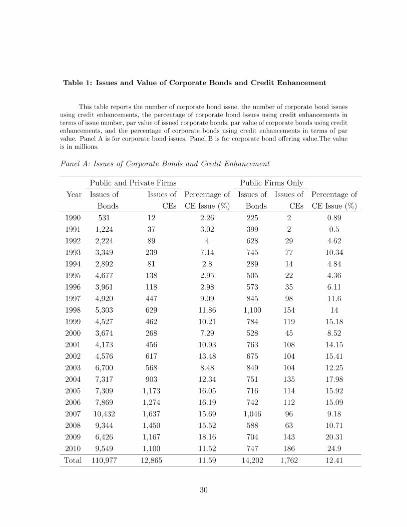
Table 1: Issues and Value of Corporate Bonds and Credit Enhancement

This table reports the number of corporate bond issue, the number of corporate bond issuesusing credit enhancements, the percentage of corporate bond issues using credit enhancements interms of issue number, par value of issued corporate bonds, par value of corporate bonds using creditenhancements, and the percentage of corporate bonds using credit enhancements in terms of parvalue. Panel A is for corporate bond issues. Panel B is for corporate bond offering value.The valueis in millions.

Panel A: Issues of Corporate Bonds and Credit Enhancement

Public and Private Firms Public Firms Only

Year Issues of Issues of Percentage of Issues of Issues of Percentage of

Bonds CEs CE Issue (%) Bonds CEs CE Issue (%)

1990 531 12 2.26 225 2 0.89

1991 1,224 37 3.02 399 2 0.5

1992 2,224 89 4 628 29 4.62

1993 3,349 239 7.14 745 77 10.34

1994 2,892 81 2.8 289 14 4.84

1995 4,677 138 2.95 505 22 4.36

1996 3,961 118 2.98 573 35 6.11

1997 4,920 447 9.09 845 98 11.6

1998 5,303 629 11.86 1,100 154 14

1999 4,527 462 10.21 784 119 15.18

2000 3,674 268 7.29 528 45 8.52

2001 4,173 456 10.93 763 108 14.15

2002 4,576 617 13.48 675 104 15.41

2003 6,700 568 8.48 849 104 12.25

2004 7,317 903 12.34 751 135 17.98

2005 7,309 1,173 16.05 716 114 15.92

2006 7,869 1,274 16.19 742 112 15.09

2007 10,432 1,637 15.69 1,046 96 9.18

2008 9,344 1,450 15.52 588 63 10.71

2009 6,426 1,167 18.16 704 143 20.31

2010 9,549 1,100 11.52 747 186 24.9

Total 110,977 12,865 11.59 14,202 1,762 12.41

30

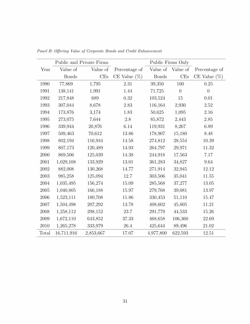
Panel B: Offering Value of Corporate Bonds and Credit Enhancement

Public and Private Firms Public Firms Only

Year Value of Value of Percentage of Value of Value of Percentage of

Bonds CEs CE Value (%) Bonds CEs CE Value (%)

1990 77,869 1,795 2.31 39,350 100 0.25

1991 138,141 1,991 1.44 71,725 0 0

1992 217,848 689 0.32 103,524 15 0.01

1993 307,044 8,678 2.83 116,164 2,930 2.52

1994 173,876 3,174 1.83 50,625 1,095 2.16

1995 273,075 7,644 2.8 85,872 2,443 2.85

1996 339,944 20,876 6.14 119,931 8,267 6.89

1997 509,463 70,612 13.86 178,907 15,180 8.48

1998 802,194 116,944 14.58 274,812 28,554 10.39

1999 807,173 120,489 14.93 264,797 29,971 11.32

2000 869,506 125,039 14.38 244,918 17,563 7.17

2001 1,029,108 133,929 13.01 361,283 34,827 9.64

2002 882,008 130,268 14.77 271,914 32,945 12.12

2003 985,258 125,094 12.7 303,506 35,041 11.55

2004 1,035,495 156,274 15.09 285,568 37,277 13.05

2005 1,040,805 166,188 15.97 279,768 39,081 13.97

2006 1,523,111 180,708 11.86 330,453 51,110 15.47

2007 1,504,498 207,292 13.78 408,602 45,805 11.21

2008 1,258,112 298,152 23.7 291,779 44,533 15.26

2009 1,672,110 643,852 37.33 468,658 106,360 22.69

2010 1,265,278 333,979 26.4 425,644 89,496 21.02

Total 16,711,916 2,853,667 17.07 4,977,800 622,593 12.51

31

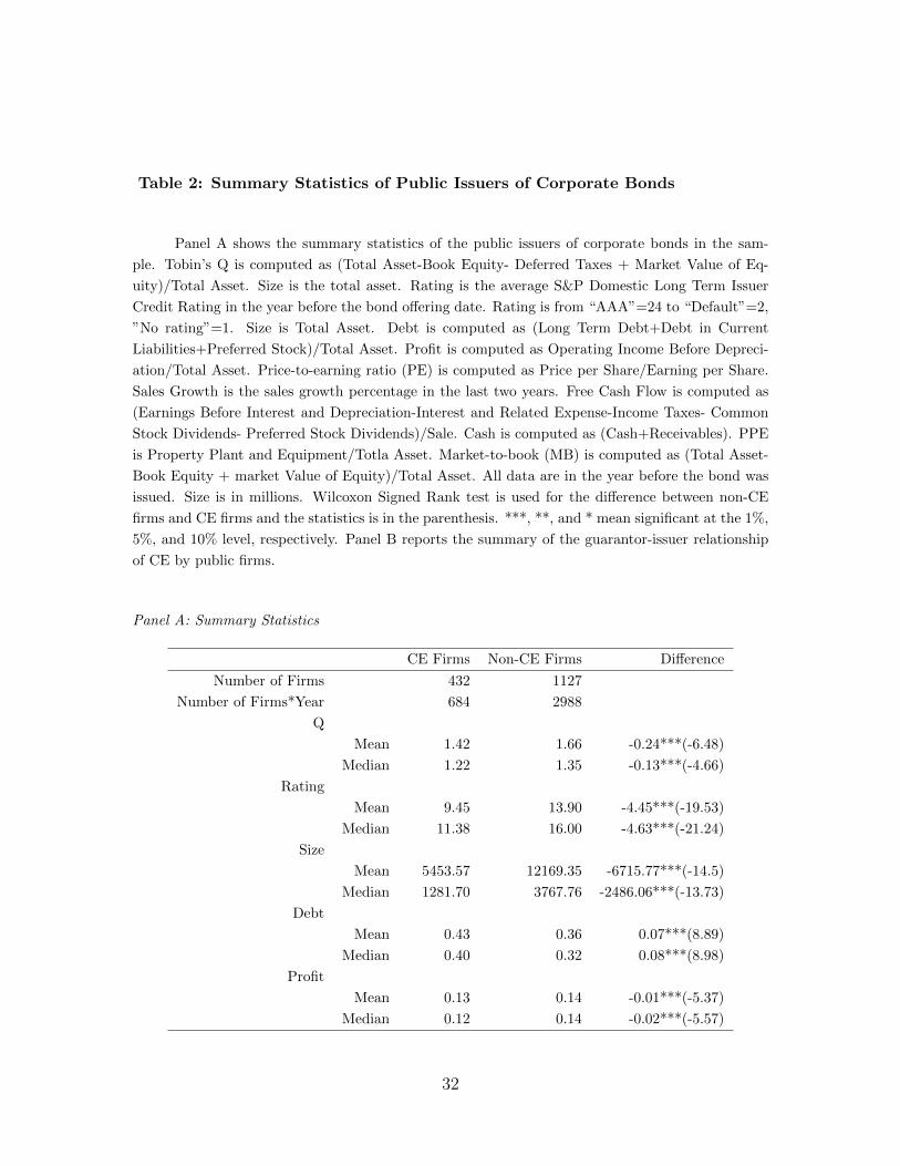
Table 2: Summary Statistics of Public Issuers of Corporate Bonds

Panel A shows the summary statistics of the public issuers of corporate bonds in the sam-

ple. Tobin’s Q is computed as (Total Asset-Book Equity- Deferred Taxes + Market Value of Eq-

uity)/Total Asset. Size is the total asset. Rating is the average S&P Domestic Long Term Issuer

Credit Rating in the year before the bond offering date. Rating is from “AAA”=24 to “Default”=2,

”No rating”=1. Size is Total Asset. Debt is computed as (Long Term Debt+Debt in Current

Liabilities+Preferred Stock)/Total Asset. Profit is computed as Operating Income Before Depreci-

ation/Total Asset. Price-to-earning ratio (PE) is computed as Price per Share/Earning per Share.

Sales Growth is the sales growth percentage in the last two years. Free Cash Flow is computed as

(Earnings Before Interest and Depreciation-Interest and Related Expense-Income Taxes- Common

Stock Dividends- Preferred Stock Dividends)/Sale. Cash is computed as (Cash+Receivables). PPE

is Property Plant and Equipment/Totla Asset. Market-to-book (MB) is computed as (Total Asset-

Book Equity + market Value of Equity)/Total Asset. All data are in the year before the bond was

issued. Size is in millions. Wilcoxon Signed Rank test is used for the difference between non-CE

firms and CE firms and the statistics is in the parenthesis. ***, **, and * mean significant at the 1%,

5%, and 10% level, respectively. Panel B reports the summary of the guarantor-issuer relationship

of CE by public firms.

Panel A: Summary Statistics

CE Firms Non-CE Firms Difference

Number of Firms 432 1127

Number of Firms*Year 684 2988

Q

Mean 1.42 1.66 -0.24***(-6.48)

Median 1.22 1.35 -0.13***(-4.66)

Rating

Mean 9.45 13.90 -4.45***(-19.53)

Median 11.38 16.00 -4.63***(-21.24)

Size

Mean 5453.57 12169.35 -6715.77***(-14.5)

Median 1281.70 3767.76 -2486.06***(-13.73)

Debt

Mean 0.43 0.36 0.07***(8.89)

Median 0.40 0.32 0.08***(8.98)

Profit

Mean 0.13 0.14 -0.01***(-5.37)

Median 0.12 0.14 -0.02***(-5.57)

32

CE Firms Non-CE Firms Difference

P/E

Mean 6.11 6.92 -0.81***(-4.66)

Median 4.76 5.58 -0.82***(-4.89)

Sales Growth

Mean 0.28 0.20 0.08***(7.44)

Median 0.16 0.09 0.07***(7.25)

Free Cash Flow

Mean 0.09 0.08 0.01(0.21)

Median 0.07 0.08 -0.01**(-2.23)

Cash

Mean 0.16 0.18 -0.02***(-3.89)

Median 0.14 0.16 -0.02***(-2.86)

Inventory

Mean 0.13 0.11 0.02 (1.51)

Median 0.06 0.08 -0.02**(-2.23)

PPE

Mean 0.63 0.69 -0.06***(-4.24)

Median 0.58 0.65 -0.07*(-1.7)

MB

Mean 1.93 2.51 -0.58***(-6.42)

Median 1.37 1.78 -0.41***(5.18)

Panel B: Guarantor-Issuer Relationship of CE by public firms

Guarantor Relationship Issue Number of CE Percentage of CEs in Terms of

by Public Firms Issue Number (%)

Subsidiaries 1395 97

Parent Firm 29 2

External Firms 8 1

33

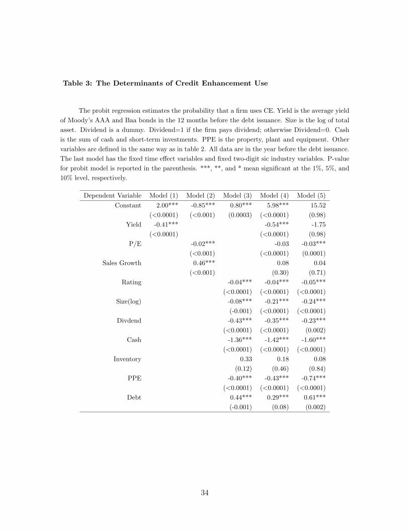
Table 3: The Determinants of Credit Enhancement Use

The probit regression estimates the probability that a firm uses CE. Yield is the average yield

of Moody’s AAA and Baa bonds in the 12 months before the debt issuance. Size is the log of total

asset. Dividend is a dummy. Dividend=1 if the firm pays dividend; otherwise Dividend=0. Cash

is the sum of cash and short-term investments. PPE is the property, plant and equipment. Other

variables are defined in the same way as in table 2. All data are in the year before the debt issuance.

The last model has the fixed time effect variables and fixed two-digit sic industry variables. P-value

for probit model is reported in the parenthesis. ***, **, and * mean significant at the 1%, 5%, and

10% level, respectively.

Dependent Variable Model (1) Model (2) Model (3) Model (4) Model (5)

Constant 2.00*** -0.85*** 0.80*** 5.98*** 15.52

(<0.0001) (<0.001) (0.0003) (<0.0001) (0.98)

Yield -0.41*** -0.54*** -1.75

(<0.0001) (<0.0001) (0.98)

P/E -0.02*** -0.03 -0.03***

(<0.001) (<0.0001) (0.0001)

Sales Growth 0.46*** 0.08 0.04

(<0.001) (0.30) (0.71)

Rating -0.04*** -0.04*** -0.05***

(<0.0001) (<0.0001) (<0.0001)

Size(log) -0.08*** -0.21*** -0.24***

(-0.001) (<0.0001) (<0.0001)

Divdend -0.43*** -0.35*** -0.23***

(<0.0001) (<0.0001) (0.002)

Cash -1.36*** -1.42*** -1.60***

(<0.0001) (<0.0001) (<0.0001)

Inventory 0.33 0.18 0.08

(0.12) (0.46) (0.84)

PPE -0.40*** -0.43*** -0.74***

(<0.0001) (<0.0001) (<0.0001)

Debt 0.44*** 0.29*** 0.61***

(-0.001) (0.08) (0.002)

34

Dependent Variable Model (1) Model (4) Model (3) Model (5) Model (6)

Profit -0.92 -1.86*** -2.21***

(-0.04) (0.001) (0.001)

Free Cash Flow 0.87*** 0.85*** 0.91**

(<0.0001) (0.001) (0.03)

Year Fixed Effect Controls No No No No Yes

Industry Fixed Effect Controls No No No No Yes

No. of observations 3672 3406 3430 3213 3211

Likehood Ratio 254.83 59.17 436.26 714.99 1039.48

Pseudo R2 0.07 0.02 0.12 0.20 0.28

35

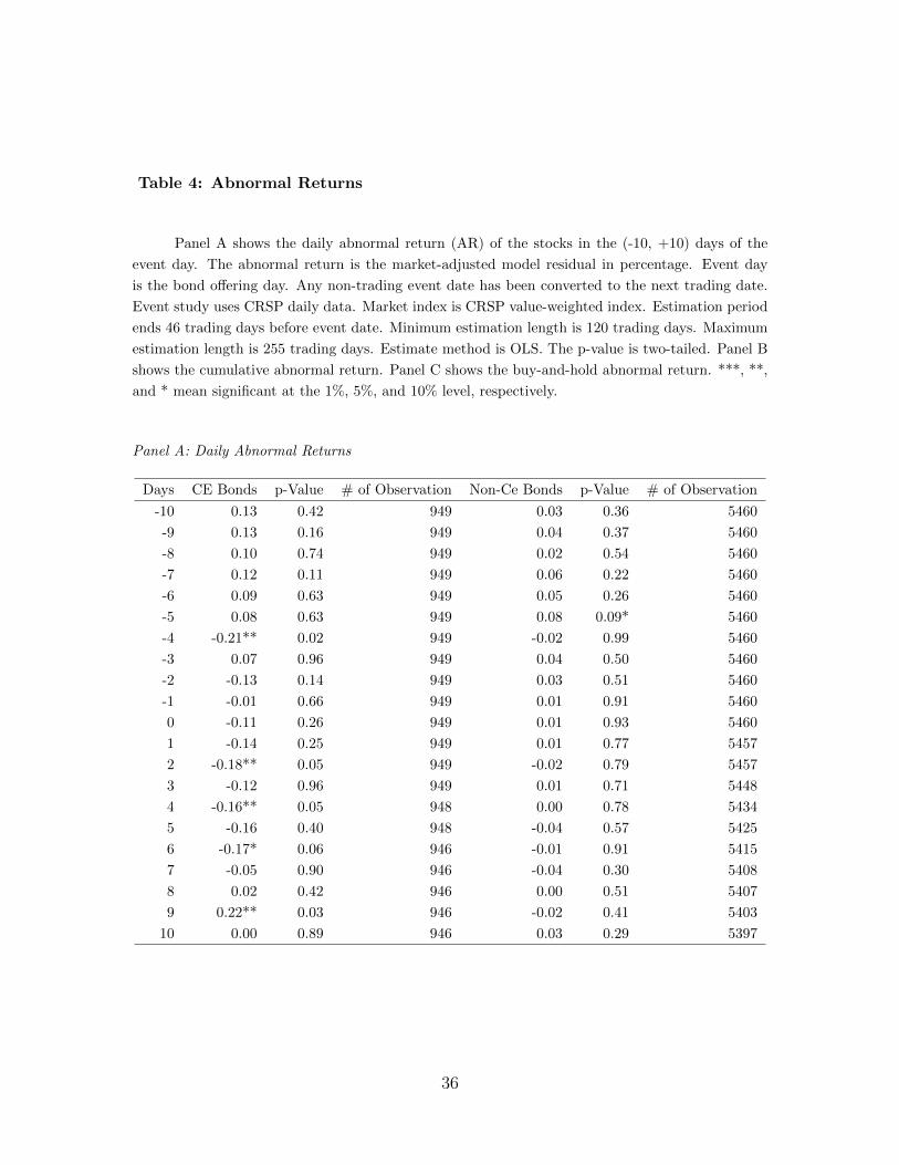
Table 4: Abnormal Returns

Panel A shows the daily abnormal return (AR) of the stocks in the (-10, +10) days of the

event day. The abnormal return is the market-adjusted model residual in percentage. Event day

is the bond offering day. Any non-trading event date has been converted to the next trading date.

Event study uses CRSP daily data. Market index is CRSP value-weighted index. Estimation period

ends 46 trading days before event date. Minimum estimation length is 120 trading days. Maximum

estimation length is 255 trading days. Estimate method is OLS. The p-value is two-tailed. Panel B

shows the cumulative abnormal return. Panel C shows the buy-and-hold abnormal return. ***, **,

and * mean significant at the 1%, 5%, and 10% level, respectively.

Panel A: Daily Abnormal Returns

Days CE Bonds p-Value # of Observation Non-Ce Bonds p-Value # of Observation

-10 0.13 0.42 949 0.03 0.36 5460

-9 0.13 0.16 949 0.04 0.37 5460

-8 0.10 0.74 949 0.02 0.54 5460

-7 0.12 0.11 949 0.06 0.22 5460

-6 0.09 0.63 949 0.05 0.26 5460

-5 0.08 0.63 949 0.08 0.09* 5460

-4 -0.21** 0.02 949 -0.02 0.99 5460

-3 0.07 0.96 949 0.04 0.50 5460

-2 -0.13 0.14 949 0.03 0.51 5460

-1 -0.01 0.66 949 0.01 0.91 5460

0 -0.11 0.26 949 0.01 0.93 5460

1 -0.14 0.25 949 0.01 0.77 5457

2 -0.18** 0.05 949 -0.02 0.79 5457

3 -0.12 0.96 949 0.01 0.71 5448

4 -0.16** 0.05 948 0.00 0.78 5434

5 -0.16 0.40 948 -0.04 0.57 5425

6 -0.17* 0.06 946 -0.01 0.91 5415

7 -0.05 0.90 946 -0.04 0.30 5408

8 0.02 0.42 946 0.00 0.51 5407

9 0.22** 0.03 946 -0.02 0.41 5403

10 0.00 0.89 946 0.03 0.29 5397

36

Panel B: Cumulative Abnormal Return

Event Window CE Bonds p-Value # of Observation Non-Ce Bonds p-Value # of Observation

(-1,1) -0.26 0.12 949 0.03 0.98 5457

(-5,5) -1.07*** 0.001 948 0.12 0.46 5425

(-10,10) -0.99*** 0.01 946 0.26 0.13 5397

(-15,15) -1.14*** 0.01 946 0.12 0.99 5392

(-20,20) -2.4*** <0.0001 946 0.01 0.72 5389

(-30,30) -3.17*** <0.0001 945 -0.21 0.12 5383

Panel C: Buy-and-Hold Abnormal Return

Event Window CE Bonds p-Value # of Observation Non-Ce Bonds p-Value # of Observation

(-1,1) -0.25 0.12 949 0.03 0.96 5457

(-5,5) -1.09 0.001 948 0.10 0.46 5425

(-10,10) -1.11 0.01 946 0.22 0.13 5397

(-15,15) -1.39 0.01 946 0.05 0.99 5392

(-20,20) -2.95 <0.0001 946 -0.18 0.73 5389

(-30,30) -3.85 <0.0001 945 -0.49 0.12 5383

37

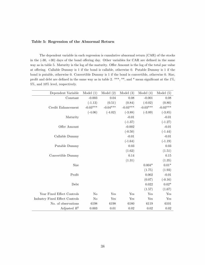
Table 5: Regression of the Abnormal Return

The dependent variable in each regression is cumulative abnormal return (CAR) of the stocks

in the (-30, +30) days of the bond offering day. Other variables for CAR are defined in the same

way as in table 5. Maturity is the log of the maturity. Offer Amount is the log of the total par value

at offering. Callable Dummy is 1 if the bond is callable, otherwise 0. Putable Dummy is 1 if the

bond is putable, otherwise 0. Convertible Dummy is 1 if the bond is convertible, otherwise 0. Size,

profit and debt are defined in the same way as in table 2. ***, **, and * mean significant at the 1%,

5%, and 10% level, respectively.

Dependent Variable Model (1) Model (2) Model (3) Model (4) Model (5)

Constant -0.003 0.04 0.08 -0.001 0.08

(-1.13) (0.51) (0.84) (-0.02) (0.80)

Credit Enhancement -0.03*** -0.04*** -0.03*** -0.03*** -0.03***

(-4.06) (-4.02) (-3.88) (-3.89) (-3.85)

Maturity -0.01 -0.01

(-1.37) (-1.27)

Offer Amount -0.002 -0.01

(-0.50) (-1.44)

Callable Dummy -0.01 -0.01

(-1.64) (-1.19)

Putable Dummy 0.03 0.03

(1.62) (1.51)

Convertible Dummy 0.14 0.15

(1.31) (1.35)

Size 0.004* 0.01*

(1.75) (1.93)

Profit 0.002 -0.01

(0.07) (-0.16)

Debt 0.022 0.02*

(1.57) (1.67)

Year Fixed Effect Controls No Yes Yes Yes Yes

Industry Fixed Effect Controls No Yes Yes Yes Yes

No. of observations 6198 6198 6180 6119 6101

Adjusted R2 0.003 0.01 0.02 0.02 0.02

38

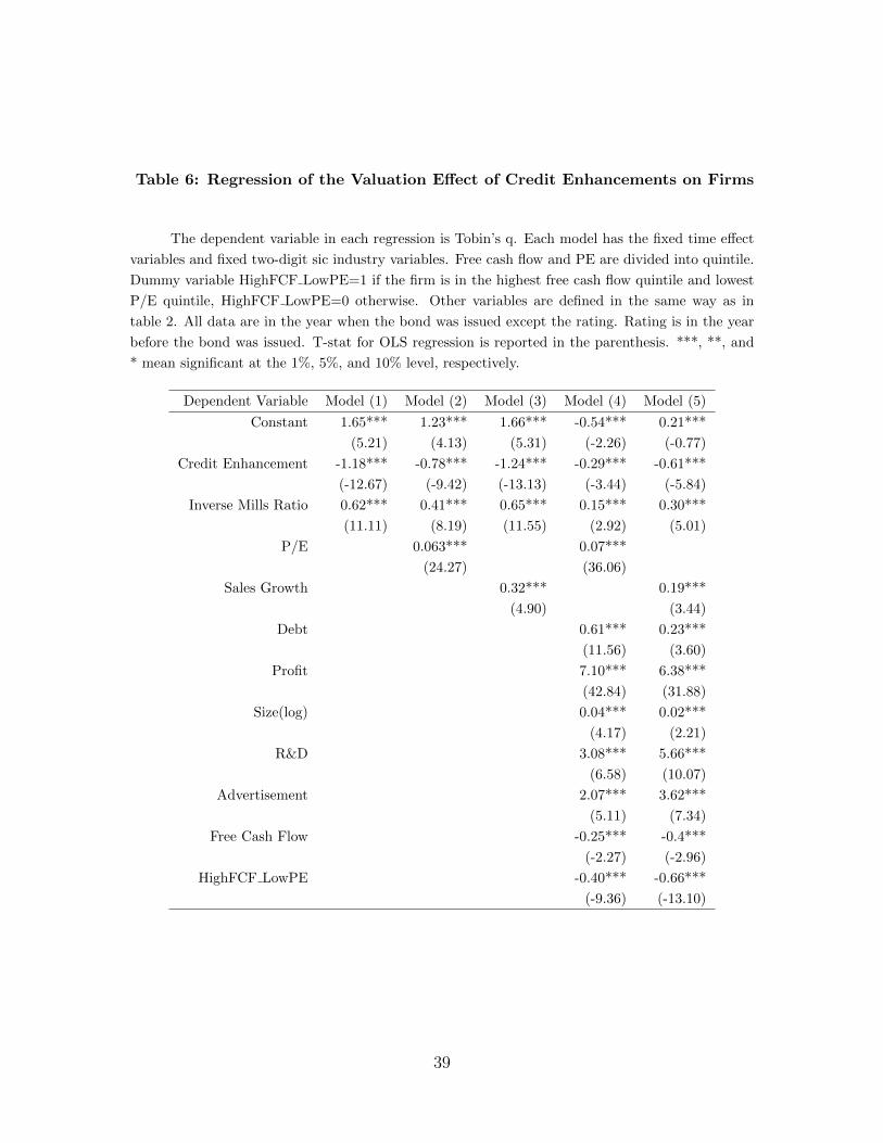
Table 6: Regression of the Valuation Effect of Credit Enhancements on Firms

The dependent variable in each regression is Tobin’s q. Each model has the fixed time effect

variables and fixed two-digit sic industry variables. Free cash flow and PE are divided into quintile.

Dummy variable HighFCF LowPE=1 if the firm is in the highest free cash flow quintile and lowest

P/E quintile, HighFCF LowPE=0 otherwise. Other variables are defined in the same way as in

table 2. All data are in the year when the bond was issued except the rating. Rating is in the year

before the bond was issued. T-stat for OLS regression is reported in the parenthesis. ***, **, and

* mean significant at the 1%, 5%, and 10% level, respectively.

Dependent Variable Model (1) Model (2) Model (3) Model (4) Model (5)

Constant 1.65*** 1.23*** 1.66*** -0.54*** 0.21***

(5.21) (4.13) (5.31) (-2.26) (-0.77)

Credit Enhancement -1.18*** -0.78*** -1.24*** -0.29*** -0.61***

(-12.67) (-9.42) (-13.13) (-3.44) (-5.84)

Inverse Mills Ratio 0.62*** 0.41*** 0.65*** 0.15*** 0.30***

(11.11) (8.19) (11.55) (2.92) (5.01)

P/E 0.063*** 0.07***

(24.27) (36.06)

Sales Growth 0.32*** 0.19***

(4.90) (3.44)

Debt 0.61*** 0.23***

(11.56) (3.60)

Profit 7.10*** 6.38***

(42.84) (31.88)

Size(log) 0.04*** 0.02***

(4.17) (2.21)

R&D 3.08*** 5.66***

(6.58) (10.07)

Advertisement 2.07*** 3.62***

(5.11) (7.34)

Free Cash Flow -0.25*** -0.4***

(-2.27) (-2.96)

HighFCF LowPE -0.40*** -0.66***

(-9.36) (-13.10)

39

Dependent Variable Model (1) Model (2) Model (3) Model (4) Model (5)

Rating -0.0015 -0.0003

(-0.71) (-0.12)

Fixed Year Effect Controls Yes Yes Yes Yes Yes

Fixed Industry Effect Controls Yes Yes Yes Yes Yes

No. of observations 2915 2915 2915 2915 2915

Adjusted R2 0.21 0.34 0.21 0.66 0.51

40

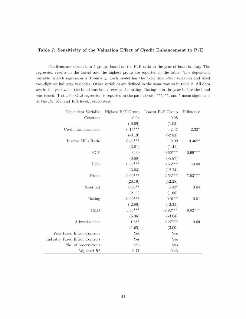
Table 7: Sensitivity of the Valuation Effect of Credit Enhancement to P/E

The firms are sorted into 5 groups based on the P/E ratio in the year of bond issuing. The

regression results in the lowest and the highest group are reported in the table. The dependent

variable in each regression is Tobin’s Q. Each model has the fixed time effect variables and fixed

two-digit sic industry variables. Other variables are defined in the same way as in table 2. All data

are in the year when the bond was issued except the rating. Rating is in the year before the bond

was issued. T-stat for OLS regression is reported in the parenthesis. ***, **, and * mean significant

at the 1%, 5%, and 10% level, respectively.

Dependent Variable Highest P/E Group Lowest P/E Group Difference

Constant -0.04 0.28

(-0.09) (1.03)

Credit Enhancement -0.15*** -2.47 2.32*

(-0.19) (-2.83)

Inverse Mills Ratio 0.45*** 0.09 0.36**

(3.01) (1.41)

FCF 0.30 -0.66*** 0.99***

(0.88) (-5.87)

Debt 0.58*** 0.66*** -0.08

(3.03) (12.24)

Profit 9.60*** 2.53*** 7.03***

(20.16) (12.28)

Size(log) 0.06** 0.02* 0.04

(2.11) (1.66)

Rating -0.02*** -0.01** -0.01

(-2.89) (-2.25)

R&D 5.36*** -2.92*** 9.82***

(5.36) (-3.64)

Advertisement 1.58* 2.27*** -0.69

(1.65) (3.00)

Year Fixed Effect Controls Yes Yes

Industry Fixed Effect Controls Yes Yes

No. of observations 583 583

Adjusted R2 0.71 0.43

41

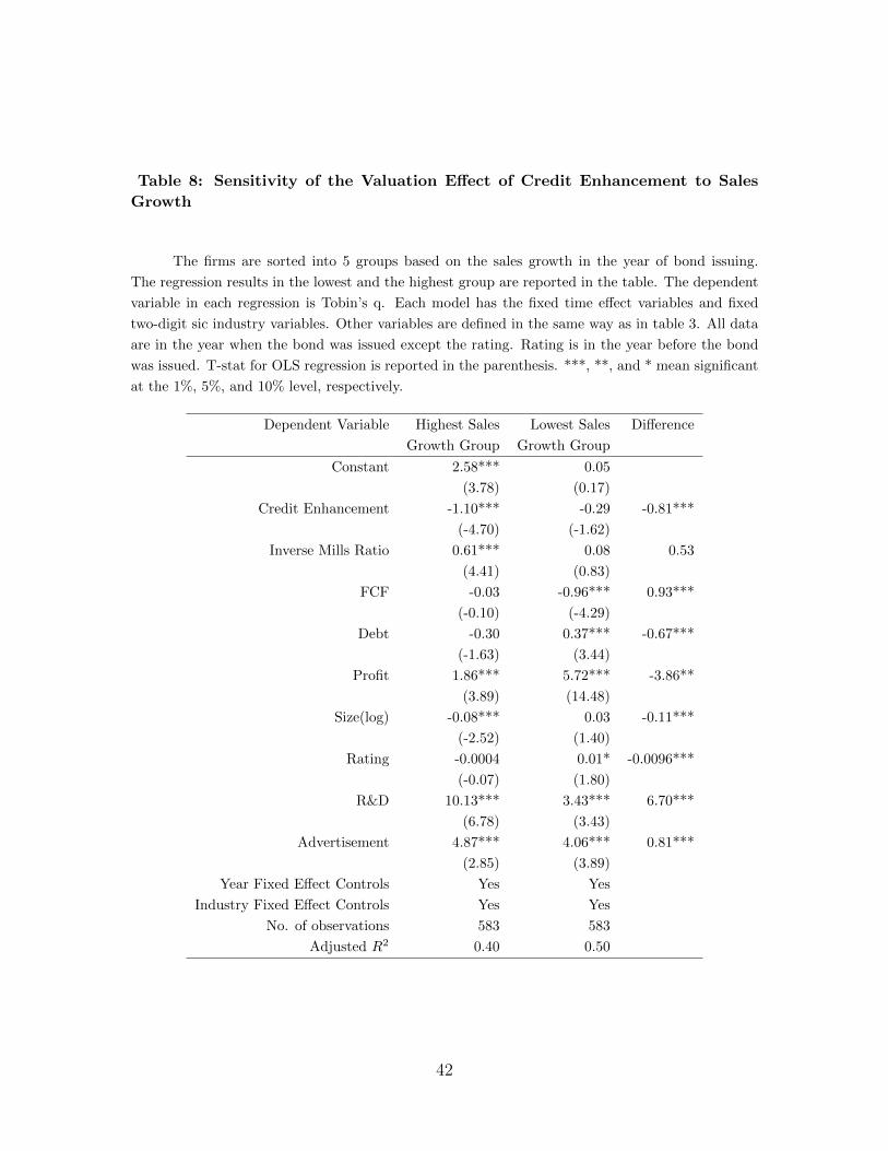
Table 8: Sensitivity of the Valuation Effect of Credit Enhancement to Sales

Growth

The firms are sorted into 5 groups based on the sales growth in the year of bond issuing.

The regression results in the lowest and the highest group are reported in the table. The dependent

variable in each regression is Tobin’s q. Each model has the fixed time effect variables and fixed

two-digit sic industry variables. Other variables are defined in the same way as in table 3. All data

are in the year when the bond was issued except the rating. Rating is in the year before the bond

was issued. T-stat for OLS regression is reported in the parenthesis. ***, **, and * mean significant

at the 1%, 5%, and 10% level, respectively.

Dependent Variable Highest Sales Lowest Sales Difference

Growth Group Growth Group

Constant 2.58*** 0.05

(3.78) (0.17)

Credit Enhancement -1.10*** -0.29 -0.81***

(-4.70) (-1.62)

Inverse Mills Ratio 0.61*** 0.08 0.53

(4.41) (0.83)

FCF -0.03 -0.96*** 0.93***

(-0.10) (-4.29)

Debt -0.30 0.37*** -0.67***

(-1.63) (3.44)

Profit 1.86*** 5.72*** -3.86**

(3.89) (14.48)

Size(log) -0.08*** 0.03 -0.11***

(-2.52) (1.40)

Rating -0.0004 0.01* -0.0096***

(-0.07) (1.80)

R&D 10.13*** 3.43*** 6.70***

(6.78) (3.43)

Advertisement 4.87*** 4.06*** 0.81***

(2.85) (3.89)

Year Fixed Effect Controls Yes Yes

Industry Fixed Effect Controls Yes Yes

No. of observations 583 583

Adjusted R2 0.40 0.50

42

Table 9: Sensitivity of the Valuation Effect of Credit Enhancement to Debt

The firms are sorted into 5 groups based on the debt level in the year of bond issuing. The

regression results in the lowest and the highest group are reported in the table. The dependent

variable in each regression is Tobin’s q. Lambda is the inverse Mills ratio in the Heckman model.

Each model has the fixed time effect variables and fixed two-digit sic industry variables. Other

variables are defined in the same way as in table 3. All data are in the year when the bond was

issued except the rating. Rating is in the year before the bond was issued. T-stat for OLS regression

is reported in the parenthesis. ***, **, and * mean significant at the 1%, 5%, and 10% level,

respectively.

Dependent Variable Highest Debt Group Lowest Debt Group Difference

Constant 0.42 -0.97

(1.36) (-2.88)

Credit Enhancement -0.66*** -1.28*** 0.62

(-0.70) (-1.83)

Inverse Mills Ratio 0.40*** 0.45*** -0.05**

(3.65) (2.89)

P/E 0.05*** 0.08*** -0.03***

(11.95) (15.45)

Sales Growth -0.02 0.06 -0.08

(-0.26) (0.41)

Profit 5.40*** 7.72*** -2.32***

(14.55) (18.21)

Size(log) -0.02 0.04 -0.06***

(-0.97) (1.61)

Rating -0.005 0.001 -0.006***

(-1.03) (0.23)

R&D 3.52*** 1.77* 1.75

(2.70) (1.87)

Advertisement 2.45*** 1.43 1.02

(2.72) (1.41)

Free Cash Flow -0.49*** -0.05

(-2.95) (-0.14)

Year Fixed Effect Controls Yes Yes

Industry Fixed Effect Controls Yes Yes

No. of observations 583 583

Adjusted R2 0.56 0.70

43