Dealing with Endogeneity in Regression Models with Dynamic...
105
Foundations and Trends R in Econometrics Vol. 3, No. 3 (2008) 165–266 c 2010 C.-J. Kim DOI: 10.1561/0800000010 Dealing with Endogeneity in Regression Models with Dynamic Coefficients By Chang-Jin Kim Contents 1 Introduction 166 2 The Control Function Approach to Dealing with Endogeneity for Models with Constant Coefficients: Basic Framework 170 2.1 The Case of i.i.d. Disturbances 170 2.2 The Case of GARCH(1,1) Disturbances 174 2.3 The Case of Serially Correlated Regressors and Disturbances 176 2.4 A Note on the Errors-in-Variables Problem in Rational Expectations Models and Moving-Average Disturbances 180 2.5 Testing for Endogeneity 182 3 Markov-Switching Models with Endogenous Regressors 183 3.1 When the Relationship Between Endogenous Variables and Instrumental Variables is Time-Invariant: Basic Idea 184
Transcript of Dealing with Endogeneity in Regression Models with Dynamic...
Foundations and Trends R© inEconometricsVol. 3, No. 3 (2008) 165–266c© 2010 C.-J. KimDOI: 10.1561/0800000010
Dealing with Endogeneity in RegressionModels with Dynamic Coefficients
By Chang-Jin Kim
Contents
1 Introduction 166
2 The Control Function Approach to Dealing withEndogeneity for Models with ConstantCoefficients: Basic Framework 170
2.1 The Case of i.i.d. Disturbances 1702.2 The Case of GARCH(1,1) Disturbances 1742.3 The Case of Serially Correlated Regressors
and Disturbances 1762.4 A Note on the Errors-in-Variables Problem in Rational
Expectations Models and Moving-Average Disturbances 1802.5 Testing for Endogeneity 182
3 Markov-Switching Models withEndogenous Regressors 183
3.1 When the Relationship Between EndogenousVariables and Instrumental Variables isTime-Invariant: Basic Idea 184
3.2 When the Relationship Between Endogenous Variablesand Instrumental Variables is Markov-Switching:A Common Latent State Variable 191
3.3 When the Relationship Between Endogenous Variablesand Instrumental Variables is Markov-Switching: TwoPotentially Correlated Latent State Variables 195
3.4 When the Relationship Between Endogenous Variablesand Instrumental Variables is Markov-Switching: FurtherGeneralization 203
3.5 Application #1: Is the Backward-Looking ComponentImportant in a New Keynesian Phillips Curve? 209
3.6 Application #2: The Nature of the Structural Break inthe Excess Sensitivity of Consumption to Income 214
4 Markov-Switching Models with EndogenousSwitching: When the State Variable andRegression Disturbance are Correlated 217
4.1 Model Specification 2184.2 Derivation of the Hamilton Filter and the Log-Likelihood
Function 2194.3 An Example in Finance: A Volatility Feedback Model of
Stock Returns 222
5 Time-Varying Parameter Models with EndogenousRegressors 228
5.1 When the Relation Between the Endogenous Variablesand Instrumental Variables is Time-Invariant 230
5.2 When the Relation Between the Endogenous Variablesand Instrumental Variables is Time-Varying 236
5.3 When the Relation Between the Endogenous Variablesand Instrumental Variables is Time-Varying: AnAlternative Two-Step Approach and a Practical SolutionWhen K is Large 242
5.4 Generalization and an Application: Estimationof a Forward-Looking Monetary Policy Rulewith Time-Varying Responses to Inflationand Output Gap 248
6 Concluding Remarks 259
References 261
Foundations and Trends R© inEconometricsVol. 3, No. 3 (2008) 165–266c© 2010 C.-J. KimDOI: 10.1561/0800000010
Dealing with Endogeneity in RegressionModels with Dynamic Coefficients
Chang-Jin Kim∗
University of Washington, USA, and Korea University, Korea,[email protected]
Abstract
The purpose of this monograph is to present a unified economet-ric framework for dealing with the issues of endogeneity in Markov-switching models and time-varying parameter models, as developed byKim (2004, 2006, 2009), Kim and Nelson (2006), Kim et al. (2008),and Kim and Kim (2009). While Cogley and Sargent (2002), Primiceri(2005), Sims and Zha (2006), and Sims et al. (2008) consider estimationof simultaneous equations models with stochastic coefficients as a sys-tem, we deal with the LIML (limited information maximum likelihood)estimation of a single equation of interest out of a simultaneous equa-tions model. Our main focus is on the two-step estimation proceduresbased on the control function approach, and we show how the problemof generated regressors can be addressed in second-step regressions.
* The author would like to thank Richard Startz and Yunmi Kim for their helpful commentsand suggestions. The author acknowledges financial support from the National ResearchFoundation of Korea (KRF-2008-342-B00006) and the Bryan C. Cressey Professorship atthe University of Washington.
1Introduction
Consider the following regression model with dynamic coefficients:
yt = x′tβt + et, et ∼ N(0,σ2
e,t), (1.1)
where yt is 1 × 1 and xt is a K × 1 vector of regressors. The K × 1vector of regression coefficients βt is stochastic and time-dependent.Depending on the assumptions on the stochastic nature of βt, we haveeither a Markov-switching model or a time-varying parameter model.For a time-varying parameter model, we conventionally assume that βt
is subject to a continuous shock. For example, we assume that:
βt = βt−1 + vt, vt ∼ i.i.d.N(0,Q), (1.2)
where the K × K matrix Q is the variance–covariance matrix of vt.For a Markov-switching model, βt is subject to a discrete shock. Forexample, we assume that βt is dependent upon a first-order, J-stateMarkov-switching process St in the following way:
βt = β1S†1,t + β2S
†2,t + . . . + βJS
†J,t, (1.3)
S†j,t =
1, if St = j; j = 1,2, . . .J
0, otherwise,(1.4)
166
167
where the transitional dynamics of St are defined as:
Pr[St = j|St−1 = i] = pji,
J∑j=1
pji = 1. (1.5)
Time-varying parameter models, which date to Cooley and Prescott(1973, 1976), Rosenberg (1973), Sarris (1973), and Markov regime-switching models, originally introduced by Goldfeld and Quandt (1973)and further extended by Hamilton (1989), and have been widely usedin modeling instability in economic relations.1 With a growing bodyof recent empirical evidence on widespread instability in macroeco-nomic relations (Diebold, 1998; Stock and Watson, 1998; Perron andQu, 2007), the importance of these time series models with dynamiccoefficients has been recognized by more macroeconomists and financialeconomists than ever before.
However, almost all applications of these models so far have beenlimited to the cases of exogenous regressors or exogenous coefficients,with the following assumptions:
Assumption #1: E(et|xt) = 0 (1.6)
Assumption #2: E(et|βt) = 0. (1.7)
When either one of the above assumptions is violated, inferencesabout the model based on the conventional Kalman (1960) filter or theconventional Hamilton (1989) filter are invalid. In particular, in thecase of endogenous regressors where Assumption #1 is violated, one istempted to employ the conventional two-step procedure. That is, defin-ing zt to be a vector of instrumental variables, one may regress xt onzt to get xt, the fitted value of xt, in the first step and then estimateEquation (1.1) by replacing xt with xt in the second step. However,this conventional two-step procedure is problematic when the regres-sion coefficients are stochastic. For example, even in the case in which etin Equation (1.1) is independent and identically distributed (i.i.d.), thedisturbance term in the second-step regression is heteroscedastic. Ignor-ing this heteroscedasticity would result in inefficiency in the two-step
1 For a comprehensive review of these models, readers are referred to Kim and Nelson (1999).
168 Introduction
estimation of the model. A more serious issue is that, unlike the caseof constant coefficients, it is not easy to solve the problem of generatedregressors in calculating the standard errors of the coefficient estima-tors.
The purpose of this monograph is to present a unified econometricframework for dealing with the issues of endogeneity in Markov-switching models and time-varying parameter models, as developedby Kim (2004, 2006, 2009), Kim and Nelson (2006), Kim et al. (2008),and Kim and Kim (2009). Note that, while Cogley and Sargent (2002),Primiceri (2005), Sims and Zha (2006), and Sims et al. (2008) considerestimation of simultaneous equations models with stochastic coeffi-cients as a system, we focus on the LIML (limited information max-imum likelihood) estimation of a single equation of interest out of asimultaneous equations model.
The control function approach, which is an econometric methodused to correct for biases that arise as a consequence of selection orendogeneity, will be the main tool in dealing with the problem of endo-geneity throughout this article. While the approach has been exten-sively applied to the sample-selection models and disequilibrium modelsin the microeconometrics literature, its application in the time-serieseconometrics literature is relatively new. The basic idea behind the con-trol function is to model the dependence of the disturbance term on theendogenous variables in a way that allows us to construct a functionsuch that, conditional on the function, the endogeneity problem in theregression equation of interest disappears. For example, in the case ofa linear regression with constant coefficients, the two-step estimationprocedure based on the control function approach proceeds as follows.In the first step, the residuals of the reduced-form equations for theendogenous regressors are estimated. Then, in the second step, the pri-mary equation of interest is estimated with these residuals included asadditional regressors.
The outline of this monograph is as follows. In Section 2, we reviewthe basic issues associated with the control function approach, whichis the main tool for dealing with endogeneity in this monograph. Weinvestigate these issues within the framework of constant regressioncoefficients. In Section 3, we consider estimation of Markov-switching
169
models with endogenous regressors, by dropping Assumption #1 inEquation (1.6) but maintaining Assumption #2 in Equation (1.7). Sec-tion 4 deals with estimation of a Markov-switching model in whichAssumption #1 is maintained but Assumption #2 is dropped. Inthis model, while the regressors are exogenous or predetermined, theMarkov-switching coefficients are correlated with regression distur-bances. The issues of endogeneity within the time-varying parametermodels are discussed in Section 5. In Sections 3–5, we will see how thebasic Hamilton (1989) filter and the basic Kalman (1960) filter can bemodified to deal with different types of endogeneity. Furthermore, wewill see how the problem of generated regressors in the two-step pro-cedure can be addressed, in light of Pagan (1984) and the results inSection 2. Finally, Section 6 provides concluding remarks.
2The Control Function Approach to Dealing with
Endogeneity for Models with ConstantCoefficients: Basic Framework
In this section, we review the basic issues related to the control functionapproach, within the framework of constant regression coefficients. Webegin our discussion with the case of i.i.d. disturbances. We then extendit to the cases of serially correlated disturbances and heteroscedasticdisturbances. The focus will be on addressing the problem of generatedregressors in two-step estimation procedures. The main results in thissection will be extended in the later sections, in order to deal with theproblem of endogeneity in Markov-switching models and time-varyingparameter models.
2.1 The Case of i.i.d. Disturbances
Consider the following linear model with endogenous regressors1:
yt = x′tβ + et, (2.1)
xt = Z ′tδ + Σ
12v v
∗t , (2.2)[
v∗t
et
]∼ i.i.d.N
([00
],
[IK ρσe
ρ′σe σ2e
]), (2.3)
1 Throughout this monograph, we will assume that all the regressors are endogenous forsimplicity of exposition.
170
2.1 The Case of i.i.d. Disturbances 171
where yt is 1 × 1; xt is a K × 1 vector of endogenous regressors;Zt = (IK ⊗ zt); zt an L × 1 vector of instrumental variables; and ρ isa K × 1 vector of correlation coefficients. We assume joint normalityof the disturbance terms as our final goal is to extend the model toincorporate time-varying or Markov-switching parameters.
The basic idea of the control function approach is to find theexpected value of yt given xt and zt, which leads to an estimatingequation containing a control function. Thus, conditional on the con-trol function, the endogeneity problem disappears. To see this, we con-sider the Cholesky decomposition of the covariance matrix of
[v∗′t et
]′in order to rewrite
[v∗′t et
]′as a function of two independent normal
shocks:[v∗t
et
]=[IK 0ρ′σe
√1 − ρ′ρσe
][ηt
εt
],
[ηt
εt
]∼ i.i.d.N(0, IK+1), (2.4)
which allow us to rewrite Equation (2.1) as follows:
yt = x′tβ + γ′v∗
t + ωt, ωt ∼ i.i.d.N(0,σ2ω), (2.5)
where γ = ρσe; σ2ω = (1 − ρ′ρ)σ2
e ; v∗t = ηt; and ωt =
√1 − ρ′ρσeεt. Here,
note that E(yt|xt,Zt) = E(yt|xt,v∗t ) = x′
tβ + γ′v∗t , and v∗
t = Σ− 1
2v (xt −
Z ′tδ) is a control function. In Equation (2.5), conditional on v∗
t , thenew disturbance term ωt is uncorrelated with either xt or v∗
t , provid-ing the justification for the following two-step procedure for consistentestimation of β:
Step 1: Estimate Equation (2.2) by ordinary least squares (OLS)and get the standardized residual, v∗
t .Step 2: Estimate the following equation by OLS:
yt = x′tβ + γv∗
t + ut, (2.6)
where v∗t in Equation (2.5) is replaced with v∗
t and u = ωt+γ′(v∗
t − v∗t ).
Note that the standard error for the estimator of β in the sec-ond step must be adjusted for the generated regressors.2 For this pur-pose, we consider the asymptotic distribution of the estimator from
2 Readers are referred to Pagan (1984) for a general discussion of the ‘problem of generatedregressors’ in two-step estimation procedures.
172 The Control Function Approach to Dealing with Endogeneity Models
the second-step regression, by assuming K = 1 and Σv = σ2v . By rewrit-
ing Equation (2.6) using matrix notations (Y = Xβ + V ∗γ + U , whereU = ω + (V ∗ − V ∗)γ), and by defining MV ∗ = IT − V ∗(V ∗′
V ∗)−1V ∗′
and PZ = Z(Z′Z)−1Z
′= Z∗(Z∗′
Z∗)−1Z∗′, where V ∗ = 1
σvV and Z∗ =
1σvZ, one can easily show that MV ∗X = PZX. Thus, we have the fol-
lowing result for the estimator of β:
β = (X ′MV ∗X)−1X ′MV ∗Y
= (X ′PZX)−1X ′PZY
= β + (X ′PZX)−1X ′PZ(ω + V ∗γ)
= β +
(1TX ′Z
(1TZ ′Z
)−1 1TZ ′X
)−1
× 1TX ′Z
(1TZ ′Z
)−1 1TZ ′ (ω + V ∗γ) p−→β, (2.7)
where the first two lines in Equation (2.7) show that the estimator forβ based on the control function approach is the same as that based onthe usual two-stage least squares method. As for the estimator of σ2
u,the variance of the disturbance term in Equation (2.6), we have:
σ2u =
1TU ′U
=1TU ′U + op(1)
=1T
(ω + (V ∗ − V ∗)γ)′(ω + (V ∗ − V ∗)γ) + op(1)
=1T
(ω + Z∗(Z∗′Z∗)−1Z∗′
V ∗γ)′(ω + Z∗(Z∗′Z∗)−1Z∗′
V ∗γ) + op(1)
=ω′ωT
+ op(1)p−→ σ2
ω. (2.8)
Furthermore, based on Equation (2.7), we can derive the followingasymptotic distribution for general K ≥ 1:
√T (β − β) d−→ N
(0,(σ2
ω + γ′γ)(plim
1TX ′MV ∗X
)−1)
≡ N
(0,σ2
e
(plim
1TX ′PZX
)−1), (2.9)
2.1 The Case of i.i.d. Disturbances 173
which, along with Equation (2.8), suggests that we can consistentlyestimate the covariance matrix of β using:
Cov(β) = (σ2u + γ′γ)(X ′MV ∗X)−1, (2.10)
where σ2u = 1
T (Y − Xβ − V ∗γ)′(Y − Xβ − V ∗γ) and γ are the esti-mators from the two-step procedure based on the control functionapproach.
The maximum likelihood method can also be applied for consis-tent estimation of the second-step regression in Equation (2.6) and forobtaining the covariance matrix of the estimated coefficients. Consis-tent estimation of the coefficients is achieved by maximizing the fol-lowing log-likelihood function:
lnL(β,γ,σ2u) =
T∑t=1
ln
[1√
2πσ2u
exp− 12σ2
u
(yt − x′tβ − γ′v∗
t )2].
(2.11)
By defining Ψ = [β′ γ′ σ2u]′ and Ψ = [β′ γ′ σ2
u]′, one might considercalculating the variance–covariance matrix of Ψ in the following usualway:
Cov1(Ψ) =[−∂
2lnL(Ψ)∂Ψ∂Ψ′ |Ψ=Ψ
]−1
. (2.12)
However, even though the variances of γ and σ2u obtained from Equa-
tion (2.12) are correct, the covariance matrix of β is incorrect. In light ofPagan’s (1984) approach. The problem of generated regressors shouldbe addressed.
Given Equations (2.9) and (2.10) and the information matrix givenbelow,
I(Ψ) =
[1
σ2u(plim 1
TX′MV ∗X) 0
0 12σ4
u
], (2.13)
which is block diagonal, the correct variance of β should be obtainedfrom the (1:K,1:K)-th block of the variance–covariance matrix of Ψcalculated in the following way:
Cov2(Ψ∗) =[−∂
2lnL(Ψ)∂Ψ∂Ψ′ |Ψ=Ψ∗
]−1
, (2.14)
174 The Control Function Approach to Dealing with Endogeneity Models
where Ψ∗ = [β′ γ′ (σ2u + γ′γ)]′. It can be easily shown that the
covariance matrix of β evaluated in this way is the same as that inEquation (2.10).
2.2 The Case of GARCH(1,1) Disturbances
Even though the above maximum likelihood approach based on thecontrol function approach does not have any advantages over the con-ventional two-stage least squares methods for the simple model given byEquations (2.1)–(2.3), it has considerable advantage when the model isextended to incorporate heteroscedasticity of known form in the distur-bances. For example, by assuming K = 1, for simplicity, let us considerthe following model with heteroscedastic disturbances:
yt = x′tβ + et, (2.15)
xt = Z ′tδ + vt, (2.16)
[v∗t
et
]≡[
vtσv,t
et
]∼ N
([00
],
[1 ρσe,t
ρσe,t σ2e,t
]), (2.17)
σ2e,t = α0,e + α1,ee
2t−1 + α2,eσ
2e,t−1, (2.18)
σ2v,t = α0,v + α1,vv
2t−1 + α2,vσ
2v,t−1, (2.19)
where the α parameters are appropriately constrained. Then theCholesky decomposition of the covariance matrix of [v∗
t et]′ leads usto rewrite Equation (2.15) as:
yt = x′tβ + γtv
∗t + ωt, ωt ∼ N(0,σ2
ω,t), (2.20)
where γt = ρσe,t; v∗t = vt
σv,t; σ2
ω,t = (1 − ρ2)σ2e,t; and ωt is uncorrelated
with either xt or v∗t .
When the forms of heteroscedasticity for the disturbance terms areunknown, one can employ the conventional two-stage least squares orthe generalized method of moments (GMM) approach to estimate β.In this case, we have no choice but to lose efficiency. With a known
2.2 The Case of GARCH(1,1) Disturbances 175
form of heteroscedasticity as in Equations (2.18) and (2.19), however,we can get efficiency gain by jointly estimating Equations (2.20) and(2.16) using the maximum likelihood estimation (MLE) procedure. Asthe disturbance terms (vt and ωt) in Equations (2.16) and (2.20) areuncorrelated, one can also employ the following two-step maximumlikelihood estimation:
Step 1: Estimate Equation (2.16) along with Equation (2.19)via the maximum likelihood estimation method, andget v∗
t = vtσv,t
, t = 1,2, . . . ,T .Step 2: Estimate Equation (2.20) along with Equation (2.18)
via the maximum likelihood estimation method byreplacing v∗
t with v∗t obtained from Step 1.
Even though the above two-step procedure provides a consistent andefficient estimator, standard errors for the estimator from the second-step regression must be adjusted for the generated regressors. Supposeσv,t and σe,t, t = 1,2, . . . ,T , are observed. By dividing both sides ofEquation (2.20) by σe,t, we get:
y∗t = x∗′
t β + ρv∗t + ω∗
t , ω∗t ∼ N(0,σ2
ω∗), (2.21)
where y∗t = yt
σe,t, x∗
t = xtσe,t
, and σ2ω∗ = 1 − ρ2. Then the second-step
regression equation is:
y∗t = x∗′
t β + ρv∗t + u∗
t , (2.22)
(Y ∗ = X∗β + V ∗ρ + U∗),
where u∗t = ω∗
t + ρ(v∗t − v∗
t ). Equation (2.22) can be estimated by OLSand the same asymptotics as in Section 2.1 can be applied, resultingthe following variance–covariance matrix of β:
√T (β − β) d−→ N
(0,(σ2
ω∗ + ρ2)(plim
1TX∗′
MV ∗X∗)−1
)
≡ N
(0,(plim
1TX∗′
MV ∗X∗)−1
), (2.23)
which gives us insight into how the correct standard error of β can beobtained from the maximum likelihood estimation of the second-step
176 The Control Function Approach to Dealing with Endogeneity Models
regression when σe,t is not observed. It is given by:
Cov(βML) = (X∗′MV ∗X
∗)−1, (2.24)
where βML is the estimate from the second-step regression MLE,MV ∗ = IT − V ∗(V ∗′
V ∗)−1V ∗′, and the rows of X∗ are given by xt
σe,t,
where σe,t is an estimate of σe,t from the second-step MLE.
2.3 The Case of Serially Correlated Regressorsand Disturbances
In a time-series regression model, suppose that the vector of regressors,which is correlated with the disturbance term, is serially correlated.In cases where the disturbance term is serially uncorrelated, the lagsof the regressors can be used as instrumental variables and consistentcoefficient estimates can be obtained by the conventional two-stageleast squares (2SLS). In case the disturbance term is serially correlatedwith AR (autoregressive) or ARMA (autoregressive moving average)dynamics, however, conventional 2SLS is not consistent because all thelagged regressors are invalid as instruments.
We consider the following regression model with endogenous regres-sors in which both the regressors and the disturbance term are seriallycorrelated:
yt = x′tβ + Wt, (2.25)
φ(L)Wt = θe(L)et, et ∼ i.i.d.N(0,σ2e), (2.26)
α(L)xt = θv(L)Σ12v v∗
t , v∗t ∼ i.i.d.N(0, IK), (2.27)
where yt is 1 × 1; xt is K × 1; all the roots of φ(L) = 0, α(L) = 0,θe(L) = 0, and θv(L) = 0 lie outside the complex unit circle. Endogene-ity in the vector xt can be specified as the following correlation structurebetween et and the standardized vt term:[
v∗t
et
]∼ i.i.d.N
([00
],
[IK ρσe
ρ′σe σ2e
]), (2.28)
where ρ is a K × 1 vector of correlation coefficients between v∗t and et.
In this setting, the conventional 2SLS estimator using lagged x
variables as instruments is inconsistent because all the lags of the x
2.3 The Case of Serially Correlated Regressors and Disturbances 177
variables are correlated with the error term Wt. However, a two-stepapproach based on the control function provides an easy solution to theproblem. By multiplying both sides of Equation (2.25) by φ(L) and byusing the orthogonal decomposition of et, we have:
φ(L)yt = φ(L)x′tβ + γ′θe(L)v∗
t + θe(L)ωt, ωt ∼ i.i.d.N(0,σ2ω),(2.29)
where γ = ρσe and σ2ω = (1 − ρ′ρ)σ2
e .Note that the term θe(L)ωt is uncorrelated with either φ(L)xt or
θe(L)v∗t in Equation (2.29). Thus, in the first step, we get v∗
t , an esti-mate of v∗
t , for t = 1,2, . . . ,T . Then in the second step, we replace v∗t
with v∗t in Equation (2.29), and estimate the resulting equation.
We employ the maximum likelihood estimation method based onthe Kalman filter and the prediction error decomposition, in order toestimate the state-space representations of the first and second-stepregression equations. In what follows, the details of the two-step esti-mation procedure are provided, under the assumption that xt is 1 × 1and that both Wt and xt are ARMA(1,1).
Step 1:
(i) We estimate the following state-space representation of Equa-tion (2.27).
Measurement Equation
xt = α1xt−1 +[1 θv,1
][ vt
vt−1
], (2.30)
(xt = α1xt−1 + Hxξx,t)
Transition Equation[vt
vt−1
]=[0 01 0
][vt−1
vt−2
]+[vt
0
],
[vt
0
]∼ i.i.d.N
([00
],
[σ2
v 00 0
]),
(2.31)
(ξx,t = Fxξx,t−1 + vt, vt ∼ i.i.d.N(0,Qx))
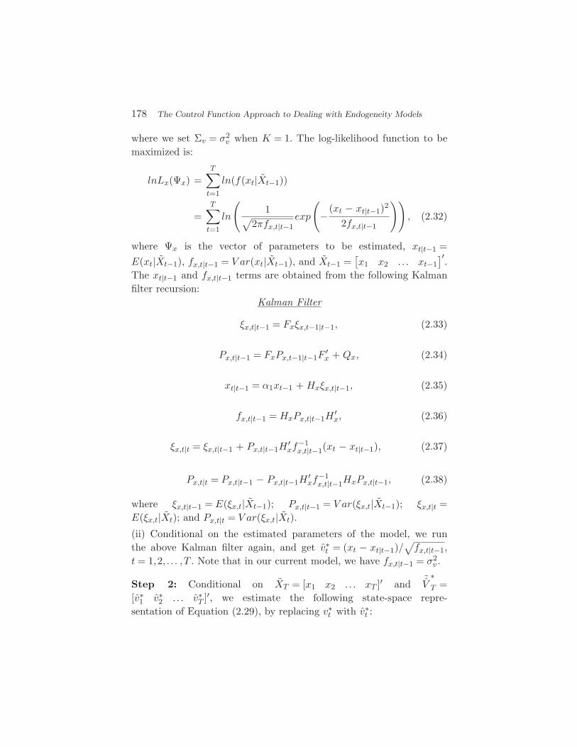
178 The Control Function Approach to Dealing with Endogeneity Models
where we set Σv = σ2v when K = 1. The log-likelihood function to be
maximized is:
lnLx(Ψx) =T∑
t=1
ln(f(xt|Xt−1))
=T∑
t=1
ln
(1√
2πfx,t|t−1exp
(−(xt − xt|t−1)2
2fx,t|t−1
)), (2.32)
where Ψx is the vector of parameters to be estimated, xt|t−1 =E(xt|Xt−1), fx,t|t−1 = V ar(xt|Xt−1), and Xt−1 =
[x1 x2 . . . xt−1
]′.
The xt|t−1 and fx,t|t−1 terms are obtained from the following Kalmanfilter recursion:
Kalman Filter
ξx,t|t−1 = Fxξx,t−1|t−1, (2.33)
Px,t|t−1 = FxPx,t−1|t−1F′x + Qx, (2.34)
xt|t−1 = α1xt−1 + Hxξx,t|t−1, (2.35)
fx,t|t−1 = HxPx,t|t−1H′x, (2.36)
ξx,t|t = ξx,t|t−1 + Px,t|t−1H′xf
−1x,t|t−1(xt − xt|t−1), (2.37)
Px,t|t = Px,t|t−1 − Px,t|t−1H′xf
−1x,t|t−1HxPx,t|t−1, (2.38)
where ξx,t|t−1 = E(ξx,t|Xt−1); Px,t|t−1 = V ar(ξx,t|Xt−1); ξx,t|t =E(ξx,t|Xt); and Px,t|t = V ar(ξx,t|Xt).
(ii) Conditional on the estimated parameters of the model, we runthe above Kalman filter again, and get v∗
t = (xt − xt|t−1)/√fx,t|t−1,
t = 1,2, . . . ,T . Note that in our current model, we have fx,t|t−1 = σ2v .
Step 2: Conditional on XT = [x1 x2 . . . xT ]′ and ˜V
∗T =
[v∗1 v∗
2 . . . v∗T ]′, we estimate the following state-space repre-
sentation of Equation (2.29), by replacing v∗t with v∗
t :
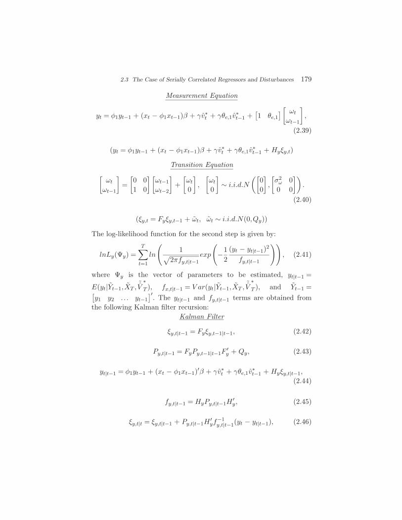
2.3 The Case of Serially Correlated Regressors and Disturbances 179
Measurement Equation
yt = φ1yt−1 + (xt − φ1xt−1)β + γv∗t + γθe,1v
∗t−1 +
[1 θe,1
][ ωt
ωt−1
],
(2.39)
(yt = φ1yt−1 + (xt − φ1xt−1)β + γv∗t + γθe,1v
∗t−1 + Hyξy,t)
Transition Equation[ωt
ωt−1
]=[0 01 0
][ωt−1
ωt−2
]+[ωt
0
],
[ωt
0
]∼ i.i.d.N
([00
],
[σ2
ω 00 0
]).
(2.40)
(ξy,t = Fyξy,t−1 + ωt, ωt ∼ i.i.d.N(0,Qy))
The log-likelihood function for the second step is given by:
lnLy(Ψy) =T∑
t=1
ln
(1√
2πfy,t|t−1exp
(−1
2(yt − yt|t−1)2
fy,t|t−1
)), (2.41)
where Ψy is the vector of parameters to be estimated, yt|t−1 =
E(yt|Yt−1, XT ,˜V
∗T ), fx,t|t−1 = V ar(yt|Yt−1, XT ,
˜V
∗T ), and Yt−1 =[
y1 y2 . . . yt−1]′
. The yt|t−1 and fy,t|t−1 terms are obtained fromthe following Kalman filter recursion:
Kalman Filter
ξy,t|t−1 = Fyξy,t−1|t−1, (2.42)
Py,t|t−1 = FyPy,t−1|t−1F′y + Qy, (2.43)
yt|t−1 = φ1yt−1 + (xt − φ1xt−1)′β + γv∗t + γθe,1v
∗t−1 + Hyξy,t|t−1,
(2.44)
fy,t|t−1 = HyPy,t|t−1H′y, (2.45)
ξy,t|t = ξy,t|t−1 + Py,t|t−1H′yf
−1y,t|t−1(yt − yt|t−1), (2.46)
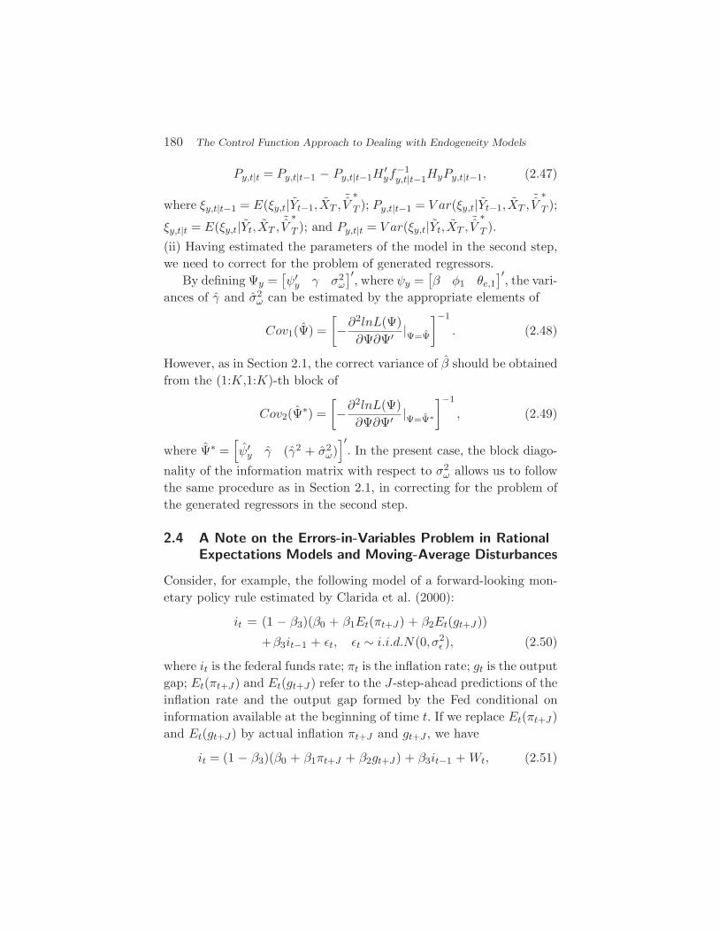
180 The Control Function Approach to Dealing with Endogeneity Models
Py,t|t = Py,t|t−1 − Py,t|t−1H′yf
−1y,t|t−1HyPy,t|t−1, (2.47)
where ξy,t|t−1 = E(ξy,t|Yt−1, XT ,˜V
∗T ); Py,t|t−1 = V ar(ξy,t|Yt−1, XT ,
˜V
∗T );
ξy,t|t = E(ξy,t|Yt, XT ,˜V
∗T ); and Py,t|t = V ar(ξy,t|Yt, XT ,
˜V
∗T ).
(ii) Having estimated the parameters of the model in the second step,we need to correct for the problem of generated regressors.
By defining Ψy =[ψ′
y γ σ2ω
]′, where ψy =
[β φ1 θe,1
]′, the vari-
ances of γ and σ2ω can be estimated by the appropriate elements of
Cov1(Ψ) =[−∂
2lnL(Ψ)∂Ψ∂Ψ′ |Ψ=Ψ
]−1
. (2.48)
However, as in Section 2.1, the correct variance of β should be obtainedfrom the (1:K,1:K)-th block of
Cov2(Ψ∗) =[−∂
2lnL(Ψ)∂Ψ∂Ψ′ |Ψ=Ψ∗
]−1
, (2.49)
where Ψ∗ =[ψ′
y γ (γ2 + σ2ω)]′
. In the present case, the block diago-
nality of the information matrix with respect to σ2ω allows us to follow
the same procedure as in Section 2.1, in correcting for the problem ofthe generated regressors in the second step.
2.4 A Note on the Errors-in-Variables Problem in RationalExpectations Models and Moving-Average Disturbances
Consider, for example, the following model of a forward-looking mon-etary policy rule estimated by Clarida et al. (2000):
it = (1 − β3)(β0 + β1Et(πt+J) + β2Et(gt+J))
+β3it−1 + εt, εt ∼ i.i.d.N(0,σ2ε ), (2.50)
where it is the federal funds rate; πt is the inflation rate; gt is the outputgap; Et(πt+J) and Et(gt+J) refer to the J-step-ahead predictions of theinflation rate and the output gap formed by the Fed conditional oninformation available at the beginning of time t. If we replace Et(πt+J)and Et(gt+J) by actual inflation πt+J and gt+J , we have
it = (1 − β3)(β0 + β1πt+J + β2gt+J) + β3it−1 + Wt, (2.51)
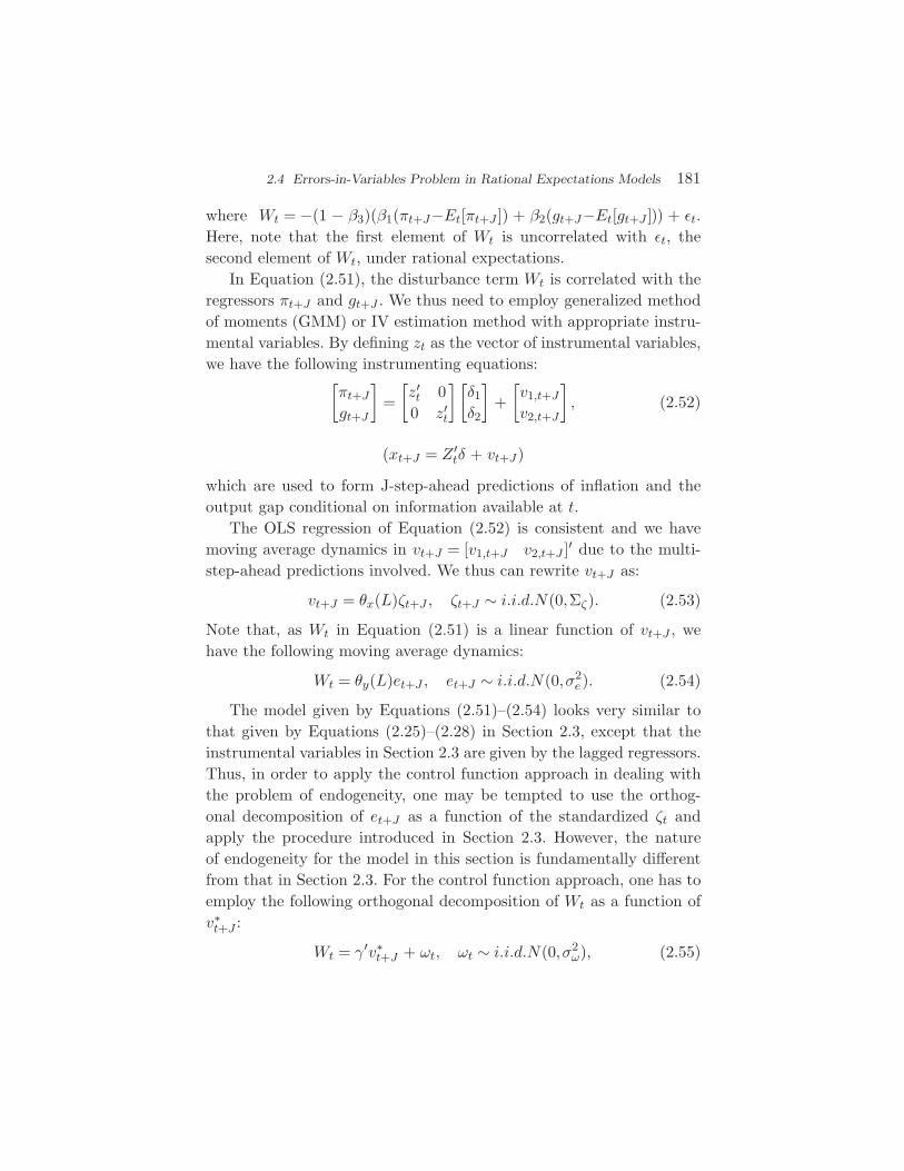
2.4 Errors-in-Variables Problem in Rational Expectations Models 181
where Wt = −(1 − β3)(β1(πt+J−Et[πt+J ]) + β2(gt+J−Et[gt+J ])) + εt.Here, note that the first element of Wt is uncorrelated with εt, thesecond element of Wt, under rational expectations.
In Equation (2.51), the disturbance term Wt is correlated with theregressors πt+J and gt+J . We thus need to employ generalized methodof moments (GMM) or IV estimation method with appropriate instru-mental variables. By defining zt as the vector of instrumental variables,we have the following instrumenting equations:[
πt+J
gt+J
]=[z′t 00 z′
t
][δ1δ2
]+[v1,t+J
v2,t+J
], (2.52)
(xt+J = Z ′tδ + vt+J)
which are used to form J-step-ahead predictions of inflation and theoutput gap conditional on information available at t.
The OLS regression of Equation (2.52) is consistent and we havemoving average dynamics in vt+J = [v1,t+J v2,t+J ]′ due to the multi-step-ahead predictions involved. We thus can rewrite vt+J as:
vt+J = θx(L)ζt+J , ζt+J ∼ i.i.d.N(0,Σζ). (2.53)
Note that, as Wt in Equation (2.51) is a linear function of vt+J , wehave the following moving average dynamics:
Wt = θy(L)et+J , et+J ∼ i.i.d.N(0,σ2e). (2.54)
The model given by Equations (2.51)–(2.54) looks very similar tothat given by Equations (2.25)–(2.28) in Section 2.3, except that theinstrumental variables in Section 2.3 are given by the lagged regressors.Thus, in order to apply the control function approach in dealing withthe problem of endogeneity, one may be tempted to use the orthog-onal decomposition of et+J as a function of the standardized ζt andapply the procedure introduced in Section 2.3. However, the natureof endogeneity for the model in this section is fundamentally differentfrom that in Section 2.3. For the control function approach, one has toemploy the following orthogonal decomposition of Wt as a function ofv∗t+J :
Wt = γ′v∗t+J + ωt, ωt ∼ i.i.d.N(0,σ2
ω), (2.55)
182 The Control Function Approach to Dealing with Endogeneity Models
where γ = ρσe, v∗t+J is standardized vt+J , and ρ is a vector of correla-
tion coefficients between et+J and v∗t+J . Note that the moving average
dynamics are completely explained by the v∗t+J term. We can thus
rewrite Equation (2.51) as:
it = (1 − β3)(β0 + β1πt+J + β2gt+J)
+β3it−1 + γ′v∗t+J + ωt, ωt ∼ i.i.d.N(0,σ2
ω), (2.56)
where ωt is uncorrelated with either v∗t+J or any of the other regressors
in Equation (2.56). This results in the following two-step procedure:
Step 1:We estimate Equation (2.52) by OLS, and save the standardized
residuals, v∗t+J .
Step 2:
(i) By replacing the v∗t+J term by v∗
t+J , we estimate Equa-tion (2.56) by the nonlinear least squares method or themaximum likelihood estimation method.
(ii) Finally, in order to solve the problem of generated regres-sors in the second step, the procedure in Section 2.1 or 2.3can be employed.
2.5 Testing for Endogeneity
An important advantage of the two-step estimation procedure basedon the control function approach is that the test of endogeneity isstraightforward. Under the null of no endogeneity (H0 : γ = 0 orH0 : ρ = 0), the second-step regression equations in all the sectionsin this manuscript do not suffer from the problem of generated regres-sors. Thus, the Wald test statistic or the likelihood ratio test statis-tic obtained from the second-step regression follows the conventionalχ2 distribution with degrees of freedom equaling the number of rowsof γ or ρ.
3Markov-Switching Models with
Endogenous Regressors
Recent decades have seen extensive interest in time-varying parame-ter models of macroeconomic and financial time series. One notableset of models are regime-switching regressions, which date to at leastQuandt (1958). Goldfeld and Quandt (1973) introduced a particularlyuseful version of these models, referred to in the following as a Markov-switching model, in which the latent state variable controlling regimeshifts follows a Markov-chain, and is thus serially dependent. In aninfluential article, Hamilton (1989) extended Markov-switching modelsto the case of dependent data, specifically an autoregression.
Since Hamilton (1989), Markov regime-switching regression modelshave been widely used in modeling instability in economic relations.However, almost all applications of these models have been limitedto the cases of exogenous or predetermined regressors. It was not untilvery recently that the problem of endogeneity in these models has beensolved by Kim (2004, 2009), based on the control function approach. Inthis section, we review the issues related to Markov-switching modelswith endogenous regressors, with a focus on two-step estimation pro-cedures and a way to deal with the problem of generated regressorsin estimating the standard errors of the coefficient estimators in thesecond step.
183
184 Markov-Switching Models with Endogenous Regressors
3.1 When the Relationship Between EndogenousVariables and Instrumental Variables isTime-Invariant: Basic Idea
We start our discussion with a simple model in which the coefficientsof the instrumenting equations are time-invariant. Consider
yt = x′tβSt + et, (3.1)
xt = Z ′tδ + Σ
12v v∗
t , (3.2)[v∗t
et
]∼ N
([00
],
[IK ρStσe,St
ρ′Stσe,St σ2
e,St
]), (3.3)
where yt is 1 × 1; xt is a K × 1 vector of endogenous variables;Zt = IK ⊗ zt, with zt being an L × 1 (L ≥ K) vector of instrumen-tal variables; ρSt is an K × 1 vector of correlation coefficients. Thesubscript St means that the corresponding parameters are dependentupon a latent discrete variable St in the following way:
θSt =J∑
j=1
θjS†j,t, (3.4)
S†j,t =
1, if St = j; j = 1,2, . . .J
0, otherwise,(3.5)
θSt = βSt , σ2St, ρSt, St = 1,2, . . . ,J.
We assume that the latent discrete variable St is independent of etor v∗
t and that it follows a first-order Markov-switching process withthe matrix of transition probabilities
P =
p11 p12 . . . p1J
p21 p22 . . . p2J...
.... . .
...pJ1 pJ2 . . . pJJ
, (3.6)
where pji = Pr[St = j|St−1 = i] and∑J
j=1 pji = 1.A key to successful estimation of the model is in the orthogonal
decomposition of et, which allows one to rewrite Equation (3.1) as:
yt = x′tβSt + γ′
Stv∗t + ωt, ωt|St ∼ i.i.d.N(0,σ2
ω,St), (3.7)
3.1 Relationship Between Endogenous Variables and Instrumental Variables 185
where γSt = ρStσe,St and σ2ω,St
= (1 − ρ′StρSt)σ2
e,St. Conditional on xt
and St, the disturbance term ωt is independent of either xt or v∗t .
3.1.1 Joint Estimation Procedure
Conditional on xt, the disturbance ωt in Equation (3.7) is indepen-dent of v∗
t in Equation (3.2). This allows us to easily derive the jointdensity of yt and xt conditional on past information and St, based onEquations (3.7) and (3.2). The resulting log-likelihood function for jointestimation of the model is given by:
lnL = ln(f(YT , XT ))
=T∑
t=1
ln(f(yt,xt|Xt−1, Yt−1))
=T∑
t=1
ln
(J∑
St=1
f(yt,xt|St, Xt−1, Yt−1)f(St|Xt−1, Yt−1)
)
=T∑
t=1
ln
(J∑
St=1
(f(yt|St, Xt, Yt−1)f(xt|Xt−1)f(St|Xt−1, Yt−1))
),
(3.8)
where Xτ = [x1 x2 . . . xτ ]′, and Yτ = [y1 y2 . . . yτ ]′. FromEquation (3.2), we have
f(xt|Xt−1) = (2π)− K2 |Σv|− 1
2 exp
(−1
2(xt − Z ′
tδ)′Σ−1
v (xt − Z ′tδ)),
(3.9)
and from Equation (3.7), we have
f(yt|St, Xt, Yt−1)
=1√
2πσ2ω,St
exp
−(yt − x′
tβSt − γ′St
Σ− 1
2v (xt − Z ′
tδ))2
2σ2ω,St
. (3.10)
In what follows, we derive the usual Hamilton filter, which providesus with a procedure for evaluating the log-likelihood function for themaximum likelihood estimation of the model and for making inferences
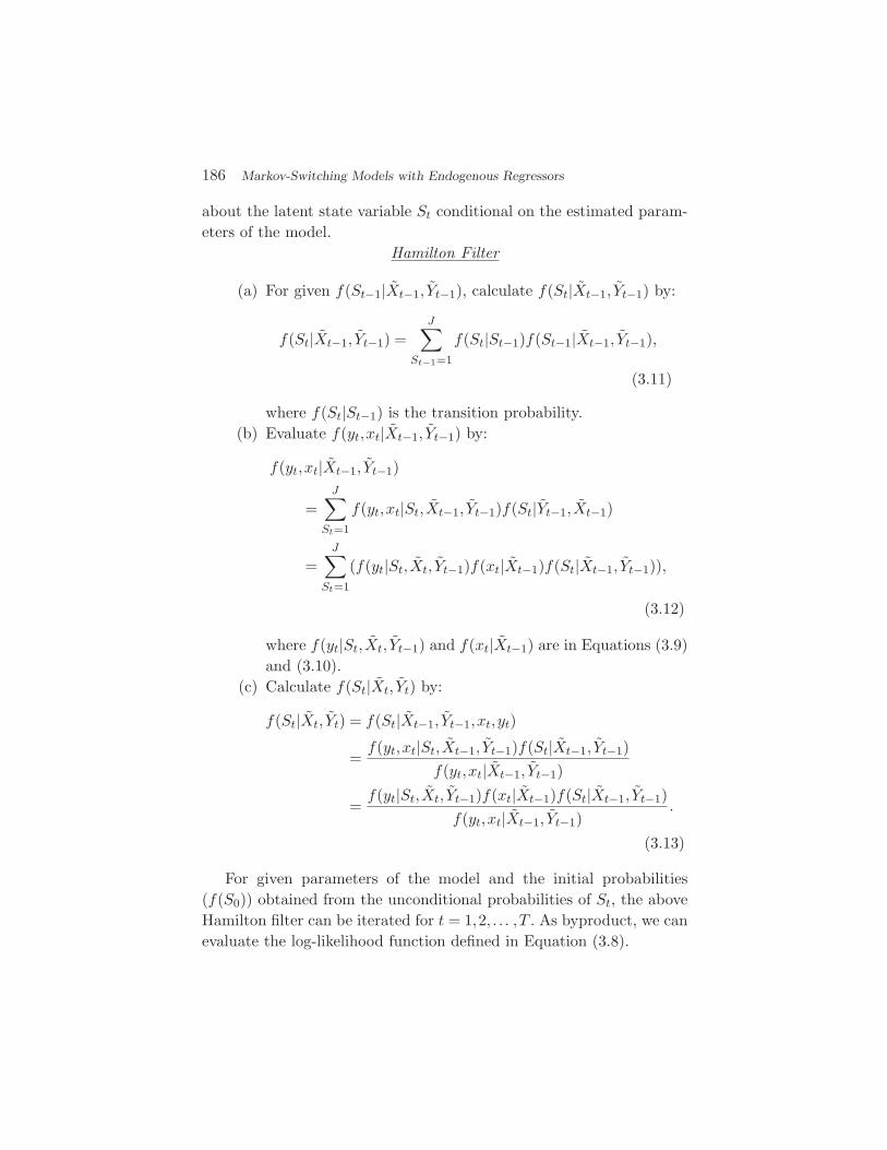
186 Markov-Switching Models with Endogenous Regressors
about the latent state variable St conditional on the estimated param-eters of the model.
Hamilton Filter
(a) For given f(St−1|Xt−1, Yt−1), calculate f(St|Xt−1, Yt−1) by:
f(St|Xt−1, Yt−1) =J∑
St−1=1
f(St|St−1)f(St−1|Xt−1, Yt−1),
(3.11)
where f(St|St−1) is the transition probability.(b) Evaluate f(yt,xt|Xt−1, Yt−1) by:
f(yt,xt|Xt−1, Yt−1)
=J∑
St=1
f(yt,xt|St, Xt−1, Yt−1)f(St|Yt−1, Xt−1)
=J∑
St=1
(f(yt|St, Xt, Yt−1)f(xt|Xt−1)f(St|Xt−1, Yt−1)),
(3.12)
where f(yt|St, Xt, Yt−1) and f(xt|Xt−1) are in Equations (3.9)and (3.10).
(c) Calculate f(St|Xt, Yt) by:
f(St|Xt, Yt) = f(St|Xt−1, Yt−1,xt,yt)
=f(yt,xt|St, Xt−1, Yt−1)f(St|Xt−1, Yt−1)
f(yt,xt|Xt−1, Yt−1)
=f(yt|St, Xt, Yt−1)f(xt|Xt−1)f(St|Xt−1, Yt−1)
f(yt,xt|Xt−1, Yt−1).
(3.13)
For given parameters of the model and the initial probabilities(f(S0)) obtained from the unconditional probabilities of St, the aboveHamilton filter can be iterated for t = 1,2, . . . ,T . As byproduct, we canevaluate the log-likelihood function defined in Equation (3.8).
3.1 Relationship Between Endogenous Variables and Instrumental Variables 187
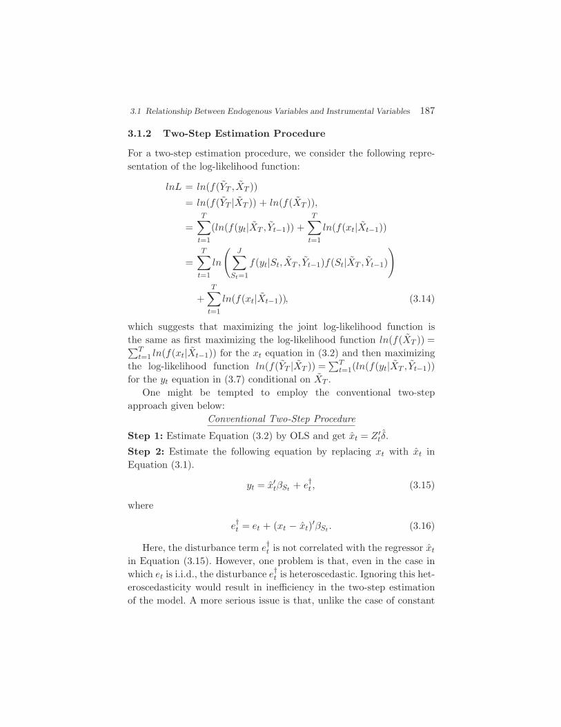
3.1.2 Two-Step Estimation Procedure
For a two-step estimation procedure, we consider the following repre-sentation of the log-likelihood function:
lnL = ln(f(YT , XT ))
= ln(f(YT |XT )) + ln(f(XT )),
=T∑
t=1
(ln(f(yt|XT , Yt−1)) +T∑
t=1
ln(f(xt|Xt−1))
=T∑
t=1
ln
(J∑
St=1
f(yt|St, XT , Yt−1)f(St|XT , Yt−1)
)
+T∑
t=1
ln(f(xt|Xt−1)), (3.14)
which suggests that maximizing the joint log-likelihood function isthe same as first maximizing the log-likelihood function ln(f(XT )) =∑T
t=1 ln(f(xt|Xt−1)) for the xt equation in (3.2) and then maximizingthe log-likelihood function ln(f(YT |XT )) =
∑Tt=1(ln(f(yt|XT , Yt−1))
for the yt equation in (3.7) conditional on XT .One might be tempted to employ the conventional two-step
approach given below:Conventional Two-Step Procedure
Step 1: Estimate Equation (3.2) by OLS and get xt = Z ′tδ.
Step 2: Estimate the following equation by replacing xt with xt inEquation (3.1).
yt = x′tβSt + e†t , (3.15)
where
e†t = et + (xt − xt)′βSt . (3.16)
Here, the disturbance term e†t is not correlated with the regressor xt
in Equation (3.15). However, one problem is that, even in the case inwhich et is i.i.d., the disturbance e†t is heteroscedastic. Ignoring this het-eroscedasticity would result in inefficiency in the two-step estimationof the model. A more serious issue is that, unlike the case of constant

188 Markov-Switching Models with Endogenous Regressors
coefficients in Section 2, it is not easy to solve the problem of generatedregressors in calculating the standard errors of the coefficient estima-tors. The two-step procedure based on the control function approach,however, does not suffer from such problems.
Two-Step Estimation Procedure based on the ControlFunction Approach
We first consider the maximum likelihood estimation of the second-step regression equation based on Equation (3.7). Note that we needthe following conditional expectation and conditional variance of yt,which is necessary to derive the Hamilton filter for Equation (3.7):
E(yt|St, XT , Yt−1) = x′tβSt + γ′
StE(v∗
t |XT ), (3.17)
V ar(yt|St, XT , Yt−1) = γ′StV ar(v∗
t |XT )γSt + σ2ω,St
. (3.18)
As the evaluation of the E(v∗t |XT ) is not easy,1 we consider esti-
mation of Equation (3.7) conditional on v∗t = v∗
t , t = 1,2, . . . ,T , wherev∗t is the standardized residual obtained from the OLS regression of
Equation (3.2). Then, we have
E(yt|St, XT ,˜V
∗T , Yt−1) = x′
tβSt + γ′Stv∗t , (3.19)
V ar(yt|St, XT ,˜V
∗T , Yt−1) = σ2
ω,St, (3.20)
where ˜V
∗T = [v∗
1 v∗2 . . . v∗
T ]′. Equations (3.19) and (3.20) will be thebasis for the derivation of the Hamilton filter for consistent estimationof the model. However, while the maximum likelihood estimation ofEquation (3.7) based on the derived Hamilton filter will provide uswith consistent estimators, the standard errors of the estimators needto be corrected for the problem of generated regressors. The followingdescribes the details of the two-step procedure based on the controlfunction approach.
Step 1:
We estimate Equation (3.2) by OLS and get the standardized residual
v∗t = Σ
− 12
v (xt − Z ′tδ).
1 This is particularly the case when the coefficients in the instrumenting equation areMarkov-switching, as in Section 3.2.
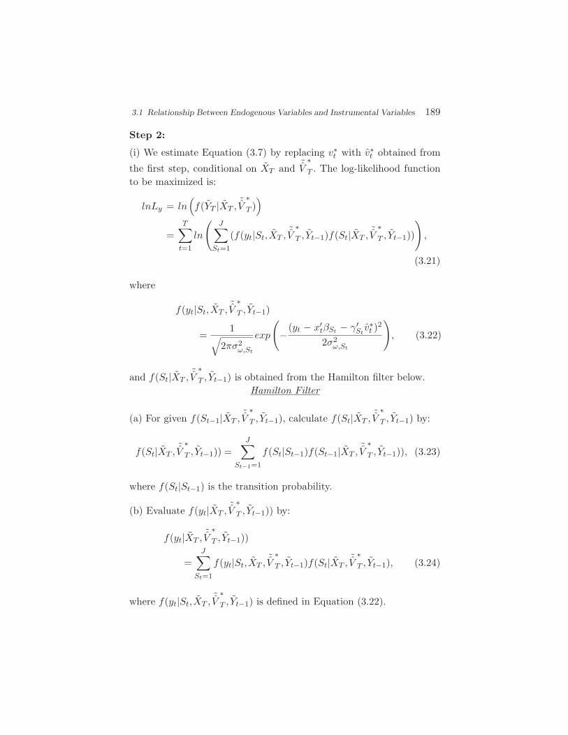
3.1 Relationship Between Endogenous Variables and Instrumental Variables 189
Step 2:
(i) We estimate Equation (3.7) by replacing v∗t with v∗
t obtained from
the first step, conditional on XT and ˜V
∗T . The log-likelihood function
to be maximized is:
lnLy = ln(f(YT |XT ,
˜V
∗T ))
=T∑
t=1
ln
(J∑
St=1
(f(yt|St, XT ,˜V
∗T , Yt−1)f(St|XT ,
˜V
∗T , Yt−1))
),
(3.21)
where
f(yt|St, XT ,˜V
∗T , Yt−1)
=1√
2πσ2ω,St
exp
(−(yt − x′
tβSt − γ′Stv∗t )
2
2σ2ω,St
), (3.22)
and f(St|XT ,˜V
∗T , Yt−1) is obtained from the Hamilton filter below.
Hamilton Filter
(a) For given f(St−1|XT ,˜V
∗T , Yt−1), calculate f(St|XT ,
˜V
∗T , Yt−1) by:
f(St|XT ,˜V
∗T , Yt−1)) =
J∑St−1=1
f(St|St−1)f(St−1|XT ,˜V
∗T , Yt−1)), (3.23)
where f(St|St−1) is the transition probability.
(b) Evaluate f(yt|XT ,˜V
∗T , Yt−1)) by:
f(yt|XT ,˜V
∗T , Yt−1))
=J∑
St=1
f(yt|St, XT ,˜V
∗T , Yt−1)f(St|XT ,
˜V
∗T , Yt−1), (3.24)
where f(yt|St, XT ,˜V
∗T , Yt−1) is defined in Equation (3.22).
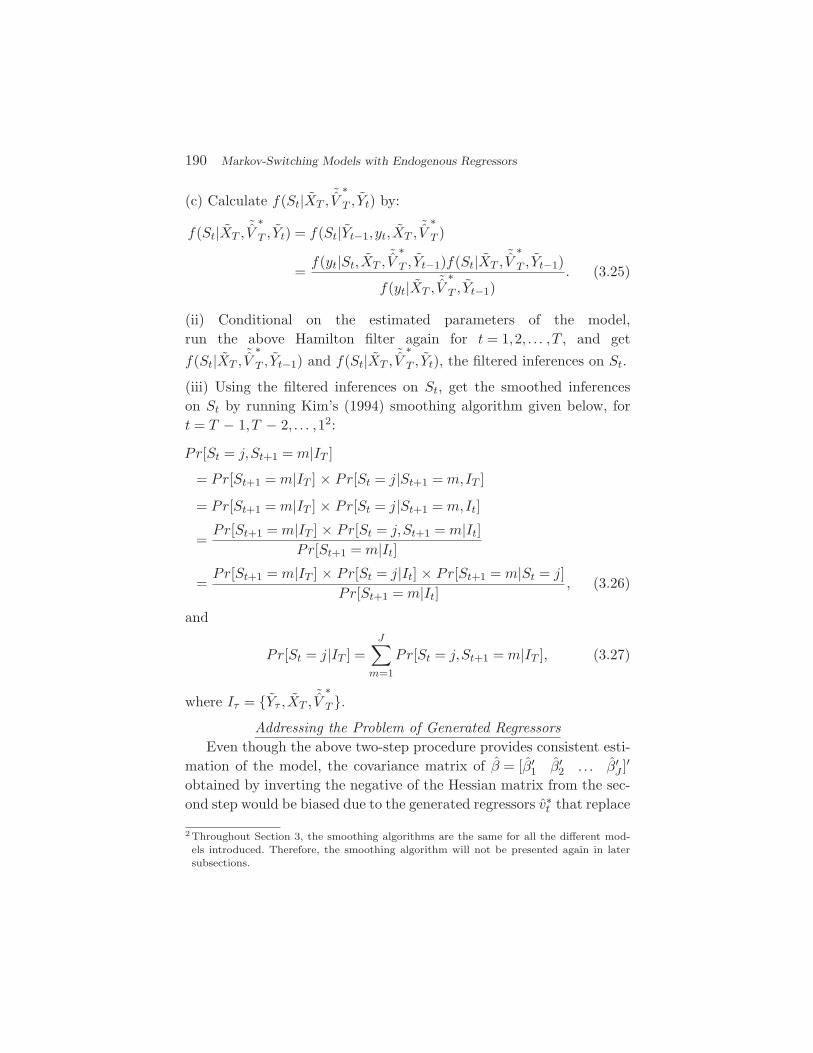
190 Markov-Switching Models with Endogenous Regressors
(c) Calculate f(St|XT ,˜V
∗T , Yt) by:
f(St|XT ,˜V
∗T , Yt) = f(St|Yt−1,yt, XT ,
˜V
∗T )
=f(yt|St, XT ,
˜V
∗T , Yt−1)f(St|XT ,
˜V
∗T , Yt−1)
f(yt|XT ,˜V
∗T , Yt−1)
. (3.25)
(ii) Conditional on the estimated parameters of the model,run the above Hamilton filter again for t = 1,2, . . . ,T , and getf(St|XT ,
˜V
∗T , Yt−1) and f(St|XT ,
˜V
∗T , Yt), the filtered inferences on St.
(iii) Using the filtered inferences on St, get the smoothed inferenceson St by running Kim’s (1994) smoothing algorithm given below, fort = T − 1,T − 2, . . . ,12:
Pr[St = j,St+1 = m|IT ]
= Pr[St+1 = m|IT ] × Pr[St = j|St+1 = m,IT ]
= Pr[St+1 = m|IT ] × Pr[St = j|St+1 = m,It]
=Pr[St+1 = m|IT ] × Pr[St = j,St+1 = m|It]
Pr[St+1 = m|It]
=Pr[St+1 = m|IT ] × Pr[St = j|It] × Pr[St+1 = m|St = j]
Pr[St+1 = m|It] , (3.26)
and
Pr[St = j|IT ] =J∑
m=1
Pr[St = j,St+1 = m|IT ], (3.27)
where Iτ = Yτ , XT ,˜V
∗T .
Addressing the Problem of Generated RegressorsEven though the above two-step procedure provides consistent esti-
mation of the model, the covariance matrix of β = [β′1 β′
2 . . . β′J ]′
obtained by inverting the negative of the Hessian matrix from the sec-ond step would be biased due to the generated regressors v∗
t that replace
2 Throughout Section 3, the smoothing algorithms are the same for all the different mod-els introduced. Therefore, the smoothing algorithm will not be presented again in latersubsections.
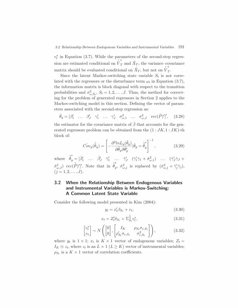
3.2 Relationship Between Endogenous Variables and Instrumental Variables 191
v∗t in Equation (3.7). While the parameters of the second-step regres-
sion are estimated conditional on ˜V
∗T and XT , the variance–covariance
matrix should be evaluated conditional on XT , but not on ˜V
∗T .
Since the latent Markov-switching state variable St is not corre-lated with the regressors or the disturbance term ωt in Equation (3.7),the information matrix is block diagonal with respect to the transitionprobabilities and σ2
ω,St, St = 1,2, . . . ,J . Thus, the method for correct-
ing for the problem of generated regressors in Section 2 applies to theMarkov-switching model in this section. Defining the vector of param-eters associated with the second-step regression as:
θy = [β′1 . . . β′
J γ′1 . . . γ′
J σ2ω,1 . . . σ2
ω,J vec(P )′]′, (3.28)
the estimator for the covariance matrix of β that accounts for the gen-erated regressors problem can be obtained from the (1 : JK,1 : JK)-thblock of:
ˆCovy(ˆθy) =
[−∂
2lnLy(θy)∂θy∂θ′
y
|θy = ˆθ
∗y
]−1
, (3.29)
where ˆθ
∗y = [β′
1 . . . β′J γ′
1 . . . γ′J (γ′
1γ1 + σ2ω,1) . . . (γ′
J γJ +
σ2ω,J) vec( ˆP )′]′. Note that in ˆ
θ∗y, σ
2ω,j is replaced by (σ2
ω,j + γ′j γj),
(j = 1,2, . . . ,J).
3.2 When the Relationship Between Endogenous Variablesand Instrumental Variables is Markov-Switching:A Common Latent State Variable
Consider the following model presented in Kim (2004):
yt = x′tβSt + et, (3.30)
xt = Z ′tδSt + Σ
12Stv∗t , (3.31)[
v∗t
et
]∼ N
([00
],
[IK ρStσe,St
ρ′Stσe,St σ2
e,St
]), (3.32)
where yt is 1 × 1; xt is K × 1 vector of endogenous variables; Zt =IK ⊗ zt, where zt is an L × 1 (L ≥ K) vector of instrumental variables;ρSt is a K × 1 vector of correlation coefficients.
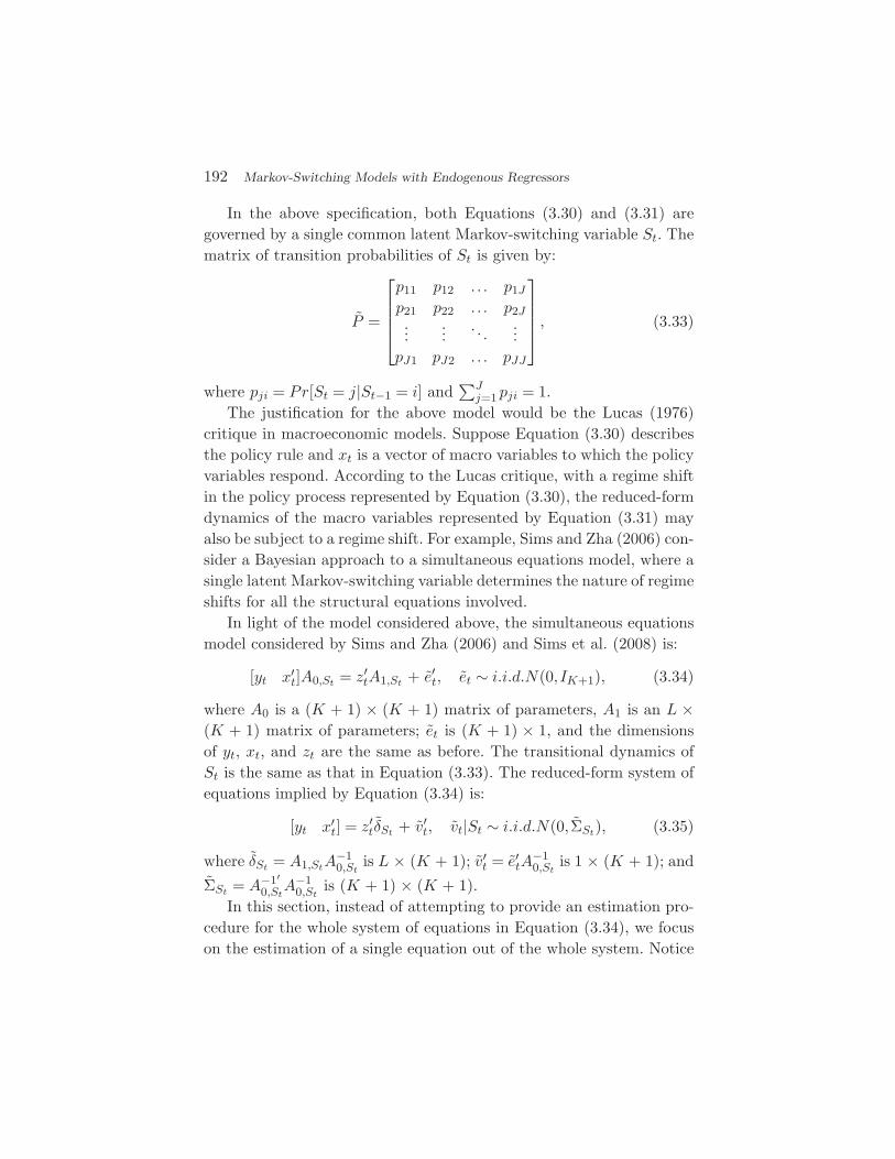
192 Markov-Switching Models with Endogenous Regressors
In the above specification, both Equations (3.30) and (3.31) aregoverned by a single common latent Markov-switching variable St. Thematrix of transition probabilities of St is given by:
P =
p11 p12 . . . p1J
p21 p22 . . . p2J...
.... . .
...pJ1 pJ2 . . . pJJ
, (3.33)
where pji = Pr[St = j|St−1 = i] and∑J
j=1 pji = 1.The justification for the above model would be the Lucas (1976)
critique in macroeconomic models. Suppose Equation (3.30) describesthe policy rule and xt is a vector of macro variables to which the policyvariables respond. According to the Lucas critique, with a regime shiftin the policy process represented by Equation (3.30), the reduced-formdynamics of the macro variables represented by Equation (3.31) mayalso be subject to a regime shift. For example, Sims and Zha (2006) con-sider a Bayesian approach to a simultaneous equations model, where asingle latent Markov-switching variable determines the nature of regimeshifts for all the structural equations involved.
In light of the model considered above, the simultaneous equationsmodel considered by Sims and Zha (2006) and Sims et al. (2008) is:
[yt x′t]A0,St = z′
tA1,St + e′t, et ∼ i.i.d.N(0, IK+1), (3.34)
where A0 is a (K + 1) × (K + 1) matrix of parameters, A1 is an L ×(K + 1) matrix of parameters; et is (K + 1) × 1, and the dimensionsof yt, xt, and zt are the same as before. The transitional dynamics ofSt is the same as that in Equation (3.33). The reduced-form system ofequations implied by Equation (3.34) is:
[yt x′t] = z′
tδSt + v′t, vt|St ∼ i.i.d.N(0, ΣSt), (3.35)
where δSt = A1,StA−10,St
is L × (K + 1); v′t = e′tA
−10,St
is 1 × (K + 1); and
ΣSt = A−1′0,St
A−10,St
is (K + 1) × (K + 1).In this section, instead of attempting to provide an estimation pro-
cedure for the whole system of equations in Equation (3.34), we focuson the estimation of a single equation out of the whole system. Notice
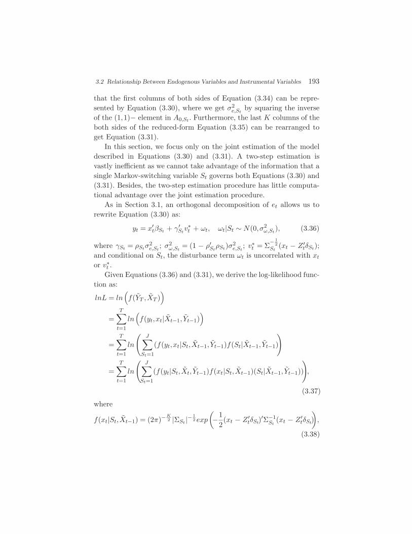
3.2 Relationship Between Endogenous Variables and Instrumental Variables 193
that the first columns of both sides of Equation (3.34) can be repre-sented by Equation (3.30), where we get σ2
e,Stby squaring the inverse
of the (1,1)− element in A0,St . Furthermore, the last K columns of theboth sides of the reduced-form Equation (3.35) can be rearranged toget Equation (3.31).
In this section, we focus only on the joint estimation of the modeldescribed in Equations (3.30) and (3.31). A two-step estimation isvastly inefficient as we cannot take advantage of the information that asingle Markov-switching variable St governs both Equations (3.30) and(3.31). Besides, the two-step estimation procedure has little computa-tional advantage over the joint estimation procedure.
As in Section 3.1, an orthogonal decomposition of et allows us torewrite Equation (3.30) as:
yt = x′tβSt + γ′
Stv∗t + ωt, ωt|St ∼ N(0,σ2
ω,St), (3.36)
where γSt = ρStσ2e,St
; σ2ω,St
= (1 − ρ′StρSt)σ2
e,St; v∗
t = Σ− 1
2St
(xt − Z ′tδSt);
and conditional on St, the disturbance term ωt is uncorrelated with xt
or v∗t .Given Equations (3.36) and (3.31), we derive the log-likelihood func-
tion as:
lnL = ln(f(YT , XT )
)
=T∑
t=1
ln(f(yt,xt|Xt−1, Yt−1)
)
=T∑
t=1
ln
(J∑
St=1
(f(yt,xt|St, Xt−1, Yt−1)f(St|Xt−1, Yt−1)
)
=T∑
t=1
ln
(J∑
St=1
(f(yt|St, Xt, Yt−1)f(xt|St, Xt−1)(St|Xt−1, Yt−1))
),
(3.37)
where
f(xt|St, Xt−1) = (2π)− K2 |ΣSt |−
12 exp
(−1
2(xt − Z ′
tδSt)′Σ−1
St(xt − Z ′
tδSt)),
(3.38)
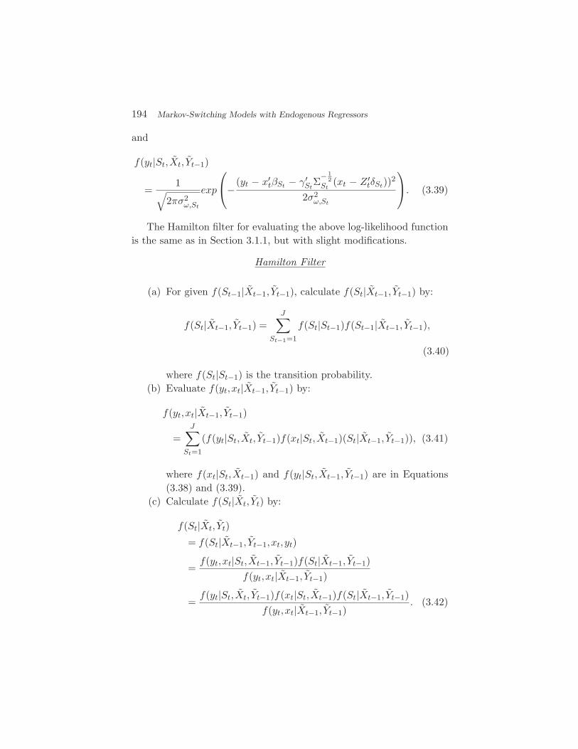
194 Markov-Switching Models with Endogenous Regressors
and
f(yt|St, Xt, Yt−1)
=1√
2πσ2ω,St
exp
−(yt − x′
tβSt − γ′St
Σ− 1
2St
(xt − Z ′tδSt))2
2σ2ω,St
. (3.39)
The Hamilton filter for evaluating the above log-likelihood functionis the same as in Section 3.1.1, but with slight modifications.
Hamilton Filter
(a) For given f(St−1|Xt−1, Yt−1), calculate f(St|Xt−1, Yt−1) by:
f(St|Xt−1, Yt−1) =J∑
St−1=1
f(St|St−1)f(St−1|Xt−1, Yt−1),
(3.40)
where f(St|St−1) is the transition probability.(b) Evaluate f(yt,xt|Xt−1, Yt−1) by:
f(yt,xt|Xt−1, Yt−1)
=J∑
St=1
(f(yt|St, Xt, Yt−1)f(xt|St, Xt−1)(St|Xt−1, Yt−1)), (3.41)
where f(xt|St, Xt−1) and f(yt|St, Xt−1, Yt−1) are in Equations(3.38) and (3.39).
(c) Calculate f(St|Xt, Yt) by:
f(St|Xt, Yt)
= f(St|Xt−1, Yt−1,xt,yt)
=f(yt,xt|St, Xt−1, Yt−1)f(St|Xt−1, Yt−1)
f(yt,xt|Xt−1, Yt−1)
=f(yt|St, Xt, Yt−1)f(xt|St, Xt−1)f(St|Xt−1, Yt−1)
f(yt,xt|Xt−1, Yt−1). (3.42)
3.3 Two Potentially Correlated Latent State Variables 195
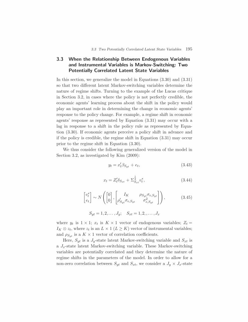
3.3 When the Relationship Between Endogenous Variablesand Instrumental Variables is Markov-Switching: TwoPotentially Correlated Latent State Variables
In this section, we generalize the model in Equations (3.30) and (3.31)so that two different latent Markov-switching variables determine thenature of regime shifts. Turning to the example of the Lucas critiquein Section 3.2, in cases where the policy is not perfectly credible, theeconomic agents’ learning process about the shift in the policy wouldplay an important role in determining the change in economic agents’response to the policy change. For example, a regime shift in economicagents’ response as represented by Equation (3.31) may occur with alag in response to a shift in the policy rule as represented by Equa-tion (3.30). If economic agents perceive a policy shift in advance andif the policy is credible, the regime shift in Equation (3.31) may occurprior to the regime shift in Equation (3.30).
We thus consider the following generalized version of the model inSection 3.2, as investigated by Kim (2009):
yt = x′tβSyt + et, (3.43)
xt = Z ′tδSxt + Σ
12Sxtv∗t , (3.44)
[v∗t
et
]∼ N
([00
],
[IK ρSytσe,Syt
ρ′Sytσe,Syt σ2
e,Syt
]), (3.45)
Syt = 1,2, . . . ,Jy; Sxt = 1,2, , . . . ,Jx
where yt is 1 × 1; xt is K × 1 vector of endogenous variables; Zt =IK ⊗ zt, where zt is an L × 1 (L ≥ K) vector of instrumental variables;and ρSyt is a K × 1 vector of correlation coefficients.
Here, Syt is a Jy-state latent Markov-switching variable and Sxt isa Jx-state latent Markov-switching variable. These Markov-switchingvariables are potentially correlated and they determine the nature ofregime shifts in the parameters of the model. In order to allow for anon-zero correlation between Syt and Sxt, we consider a Jy × Jx-state
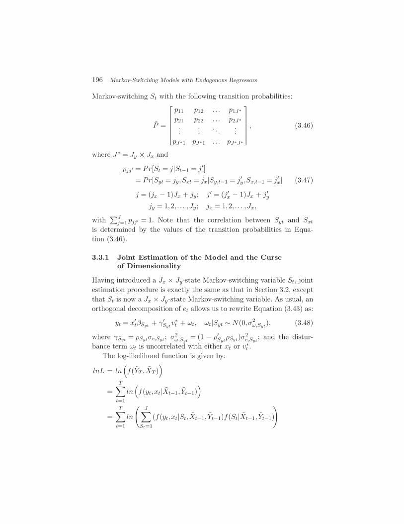
196 Markov-Switching Models with Endogenous Regressors
Markov-switching St with the following transition probabilities:
P =
p11 p12 . . . p1J∗
p21 p22 . . . p2J∗...
.... . .
...pJ∗1 pJ∗1 . . . pJ∗J∗
, (3.46)
where J∗ = Jy × Jx and
pjj′ = Pr[St = j|St−1 = j′]
= Pr[Syt = jy,Sxt = jx|Sy,t−1 = j′y,Sx,t−1 = j′
x] (3.47)
j = (jx − 1)Jx + jy; j′ = (j′x − 1)Jx + j′
y
jy = 1,2, . . . ,Jy; jx = 1,2, . . . ,Jx,
with∑J
j=1 pjj′ = 1. Note that the correlation between Syt and Sxt
is determined by the values of the transition probabilities in Equa-tion (3.46).
3.3.1 Joint Estimation of the Model and the Curseof Dimensionality
Having introduced a Jx × Jy-state Markov-switching variable St, jointestimation procedure is exactly the same as that in Section 3.2, exceptthat St is now a Jx × Jy-state Markov-switching variable. As usual, anorthogonal decomposition of et allows us to rewrite Equation (3.43) as:
yt = x′tβSyt + γ′
Sytv∗t + ωt, ωt|Syt ∼ N(0,σ2
ω,Syt), (3.48)
where γSyt = ρSytσe,Syt ; σ2ω,Syt
= (1 − ρ′SytρSyt)σ2
e,Syt; and the distur-
bance term ωt is uncorrelated with either xt or v∗t .
The log-likelihood function is given by:
lnL = ln(f(YT , XT )
)
=T∑
t=1
ln(f(yt,xt|Xt−1, Yt−1)
)
=T∑
t=1
ln
(J∑
St=1
(f(yt,xt|St, Xt−1, Yt−1)f(St|Xt−1, Yt−1)
)
3.3 Two Potentially Correlated Latent State Variables 197
=T∑
t=1
ln
(J∑
St=1
(f(yt|St, Xt, Yt−1)f(xt|St, Xt−1)(St|Xt−1, Yt−1))
)
=T∑
t=1
ln
Jx∑
Sxt=1
Jy∑Syt=1
(f(yt|Sxt,Syt, Xt, Yt−1)
× f(xt|Sxt, Xt−1)(Sxt,Syt|Xt−1, Yt−1))
, (3.49)
where
f(xt|Sxt, Xt−1)
= (2π)− K2 |ΣSxt |−
12 exp
(−1
2(xt − Z ′
tδSxt)′Σ−1
Sxt(xt − Z ′
tδSxt)), (3.50)
and
f(yt|Sxt,Syt, Xt, Yt−1)
=1√
2πσ2ω,Syt
exp
−
(yt − x′tβSyt − γ′
SytΣ
− 12
Sxt(xt − Z ′
tδSxt))2
2σ2ω,Syt
. (3.51)
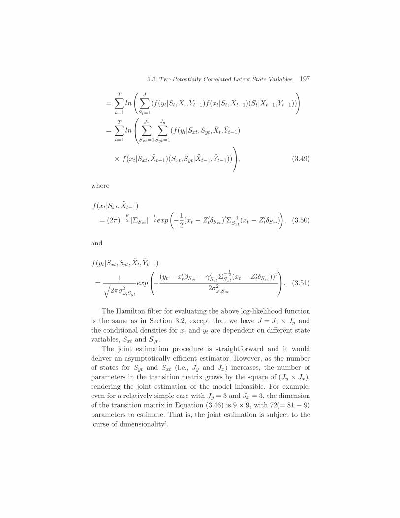
The Hamilton filter for evaluating the above log-likelihood functionis the same as in Section 3.2, except that we have J = Jx × Jy andthe conditional densities for xt and yt are dependent on different statevariables, Sxt and Syt.
The joint estimation procedure is straightforward and it woulddeliver an asymptotically efficient estimator. However, as the numberof states for Syt and Sxt (i.e., Jy and Jx) increases, the number ofparameters in the transition matrix grows by the square of (Jy × Jx),rendering the joint estimation of the model infeasible. For example,even for a relatively simple case with Jy = 3 and Jx = 3, the dimensionof the transition matrix in Equation (3.46) is 9 × 9, with 72(= 81 − 9)parameters to estimate. That is, the joint estimation is subject to the‘curse of dimensionality’.
198 Markov-Switching Models with Endogenous Regressors
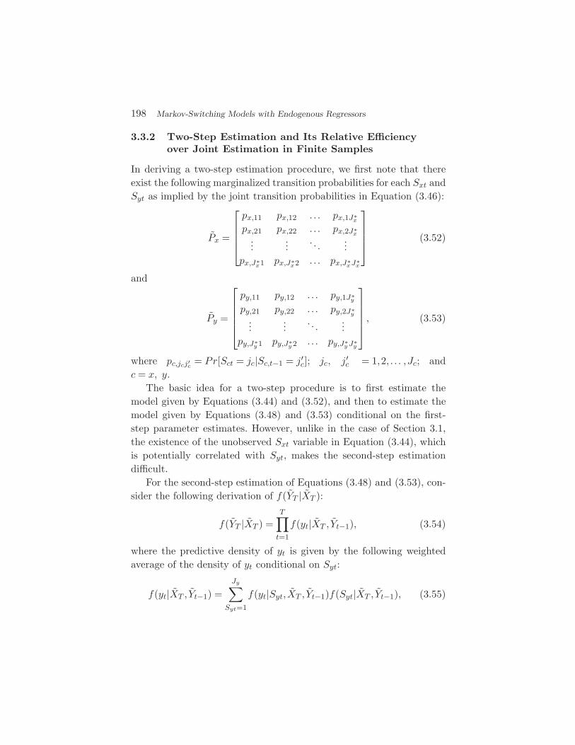
3.3.2 Two-Step Estimation and Its Relative Efficiencyover Joint Estimation in Finite Samples
In deriving a two-step estimation procedure, we first note that thereexist the following marginalized transition probabilities for each Sxt andSyt as implied by the joint transition probabilities in Equation (3.46):
Px =
px,11 px,12 . . . px,1J∗
x
px,21 px,22 . . . px,2J∗x
......
. . ....
px,J∗x1 px,J∗
x2 . . . px,J∗xJ∗
x
(3.52)
and
Py =
py,11 py,12 . . . py,1J∗
y
py,21 py,22 . . . py,2J∗y
......
. . ....
py,J∗y 1 py,J∗
y 2 . . . py,J∗y J∗
y
, (3.53)
where pc,jcj′c= Pr[Sct = jc|Sc,t−1 = j′
c]; jc, j′c = 1,2, . . . ,Jc; and
c = x, y.The basic idea for a two-step procedure is to first estimate the
model given by Equations (3.44) and (3.52), and then to estimate themodel given by Equations (3.48) and (3.53) conditional on the first-step parameter estimates. However, unlike in the case of Section 3.1,the existence of the unobserved Sxt variable in Equation (3.44), whichis potentially correlated with Syt, makes the second-step estimationdifficult.
For the second-step estimation of Equations (3.48) and (3.53), con-sider the following derivation of f(YT |XT ):
f(YT |XT ) =T∏
t=1
f(yt|XT , Yt−1), (3.54)
where the predictive density of yt is given by the following weightedaverage of the density of yt conditional on Syt:
f(yt|XT , Yt−1) =Jy∑
Syt=1
f(yt|Syt, XT , Yt−1)f(Syt|XT , Yt−1), (3.55)
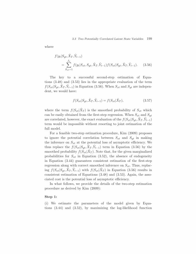
3.3 Two Potentially Correlated Latent State Variables 199
where
f(yt|Syt, XT , Yt−1)
=Jx∑
Sxt=1
f(yt|Sxt,Syt, XT , Yt−1)f(Sxt|Syt, XT , Yt−1). (3.56)
The key to a successful second-step estimation of Equa-tions (3.48) and (3.53) lies in the appropriate evaluation of the termf(Sxt|Syt, XT , Yt−1) in Equation (3.56). When Sxt and Syt are indepen-dent, we would have:
f(Sxt|Syt, XT , Yt−1) = f(Sxt|XT ), (3.57)
where the term f(Sxt|XT ) is the smoothed probability of Sxt whichcan be easily obtained from the first-step regression. When Sxt and Syt
are correlated, however, the exact evaluation of the f(Sxt|Syt, XT , Yt−1)term would be impossible without resorting to joint estimation of thefull model.
For a feasible two-step estimation procedure, Kim (2009) proposesto ignore the potential correlation between Sxt and Syt in makingthe inference on Sxt at the potential loss of asymptotic efficiency. Wethus replace the f(Sxt|Syt, XT , Yt−1) term in Equation (3.56) by thesmoothed probability f(Sxt|XT ). Note that, for the given marginalizedprobabilities for Sxt in Equation (3.52), the absence of endogeneityin Equation (3.44) guarantees consistent estimation of the first-stepregression along with correct smoothed inference on Sxt. Thus, replac-ing f(Sxt|Syt, XT , Yt−1) with f(Sxt|XT ) in Equation (3.56) results inconsistent estimation of Equations (3.48) and (3.53). Again, the asso-ciated cost is the potential loss of asymptotic efficiency.
In what follows, we provide the details of the two-step estimationprocedure as derived by Kim (2009):
Step 1:
(i) We estimate the parameters of the model given by Equa-tions (3.44) and (3.52), by maximizing the log-likelihood function
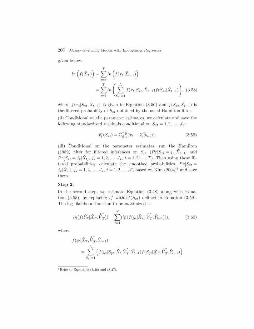
200 Markov-Switching Models with Endogenous Regressors
given below.
ln(f(XT )
)=
T∑t=1
ln(f(xt|Xt−1)
)
=T∑
t=1
ln
(Jx∑
Sxt=1
f(xt|Sxt, Xt−1)f(Sxt|Xt−1)
), (3.58)
where f(xt|Sxt, Xt−1) is given in Equation (3.50) and f(Sxt|Xt−1) isthe filtered probability of Sxt obtained by the usual Hamilton filter.
(ii) Conditional on the parameter estimates, we calculate and save thefollowing standardized residuals conditional on Sxt = 1,2, . . . ,Jx:
v∗t (Sxt) = Σ
− 12
Sxt(xt − Z ′
tδSxt)). (3.59)
(iii) Conditional on the parameter estimates, run the Hamilton(1989) filter for filtered inferences on Sxt (Pr[Sxt = jx|Xt−1] andPr[Sxt = jx|Xt], jx = 1,2, . . . ,Jx, t = 1,2, . . . ,T ). Then using these fil-tered probabilities, calculate the smoothed probabilities, Pr[Sxt =jx|XT ], jx = 1,2, . . . ,Jx, t = 1,2, . . . ,T , based on Kim (2004)3 and savethem.
Step 2:
In the second step, we estimate Equation (3.48) along with Equa-tion (3.53), by replacing v∗
t with v∗t (Sxt) defined in Equation (3.59).
The log-likelihood function to be maximized is:
ln(f(YT |XT ,˜V
∗T )) =
T∑t=1
(ln(f(yt|XT ,˜V
∗T , Yt−1))), (3.60)
where
f(yt|XT ,˜V
∗T , Yt−1)
=Jy∑
Syt=1
(f(yt|Syt, Xt,
˜V
∗T , Yt−1)f(Syt|XT ,
˜V
∗T , Yt−1)
)
3 Refer to Equations (3.26) and (3.27).
3.3 Two Potentially Correlated Latent State Variables 201
=Jy∑
Syt=1
(Jx∑
Sxt=1
(f(yt|Sxt,Syt, XT ,˜V
∗T , Yt−1)f(Sxt|XT ))
× f(Syt|XT ,˜V
∗T , Yt−1)
), (3.61)
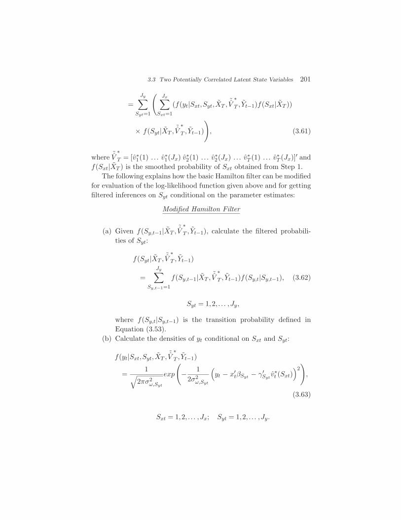
where ˜V
∗T = [v∗
1(1) . . . v∗1(Jx) v∗
2(1) . . . v∗2(Jx) . . . v∗
T (1) . . . v∗T (Jx)]′ and
f(Sxt|XT ) is the smoothed probability of Sxt obtained from Step 1.The following explains how the basic Hamilton filter can be modified
for evaluation of the log-likelihood function given above and for gettingfiltered inferences on Syt conditional on the parameter estimates:
Modified Hamilton Filter
(a) Given f(Sy,t−1|XT ,˜V
∗T , Yt−1), calculate the filtered probabili-
ties of Syt:
f(Syt|XT ,˜V
∗T , Yt−1)
=Jy∑
Sy,t−1=1
f(Sy,t−1|XT ,˜V
∗T , Yt−1)f(Sy,t|Sy,t−1), (3.62)
Syt = 1,2, . . . ,Jy,
where f(Sy,t|Sy,t−1) is the transition probability defined inEquation (3.53).
(b) Calculate the densities of yt conditional on Sxt and Syt:
f(yt|Sxt,Syt, XT ,˜V
∗T , Yt−1)
=1√
2πσ2ω,Syt
exp
(− 1
2σ2ω,Syt
(yt − x′
tβSyt − γ′Sytv∗t (Sxt)
)2),
(3.63)
Sxt = 1,2, . . . ,Jx; Syt = 1,2, . . . ,Jy.
202 Markov-Switching Models with Endogenous Regressors
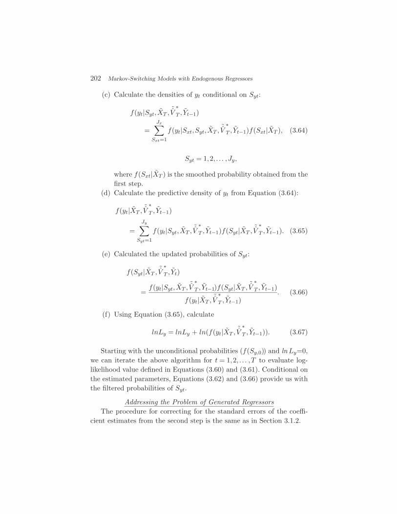
(c) Calculate the densities of yt conditional on Syt:
f(yt|Syt, XT ,˜V
∗T , Yt−1)
=Jx∑
Sxt=1
f(yt|Sxt,Syt, XT ,˜V
∗T , Yt−1)f(Sxt|XT ), (3.64)
Syt = 1,2, . . . ,Jy,
where f(Sxt|XT ) is the smoothed probability obtained from thefirst step.
(d) Calculate the predictive density of yt from Equation (3.64):
f(yt|XT ,˜V
∗T , Yt−1)
=Jy∑
Syt=1
f(yt|Syt, XT ,˜V
∗T , Yt−1)f(Syt|XT ,
˜V
∗T , Yt−1). (3.65)
(e) Calculated the updated probabilities of Syt:
f(Syt|XT ,˜V
∗T , Yt)
=f(yt|Syt, XT ,
˜V
∗T , Yt−1)f(Syt|XT ,
˜V
∗T , Yt−1)
f(yt|XT ,˜V
∗T , Yt−1)
. (3.66)
(f) Using Equation (3.65), calculate
lnLy = lnLy + ln(f(yt|XT ,˜V
∗T , Yt−1)). (3.67)
Starting with the unconditional probabilities (f(Sy,0)) and lnLy=0,we can iterate the above algorithm for t = 1,2, . . . ,T to evaluate log-likelihood value defined in Equations (3.60) and (3.61). Conditional onthe estimated parameters, Equations (3.62) and (3.66) provide us withthe filtered probabilities of Syt.
Addressing the Problem of Generated RegressorsThe procedure for correcting for the standard errors of the coeffi-
cient estimates from the second step is the same as in Section 3.1.2.
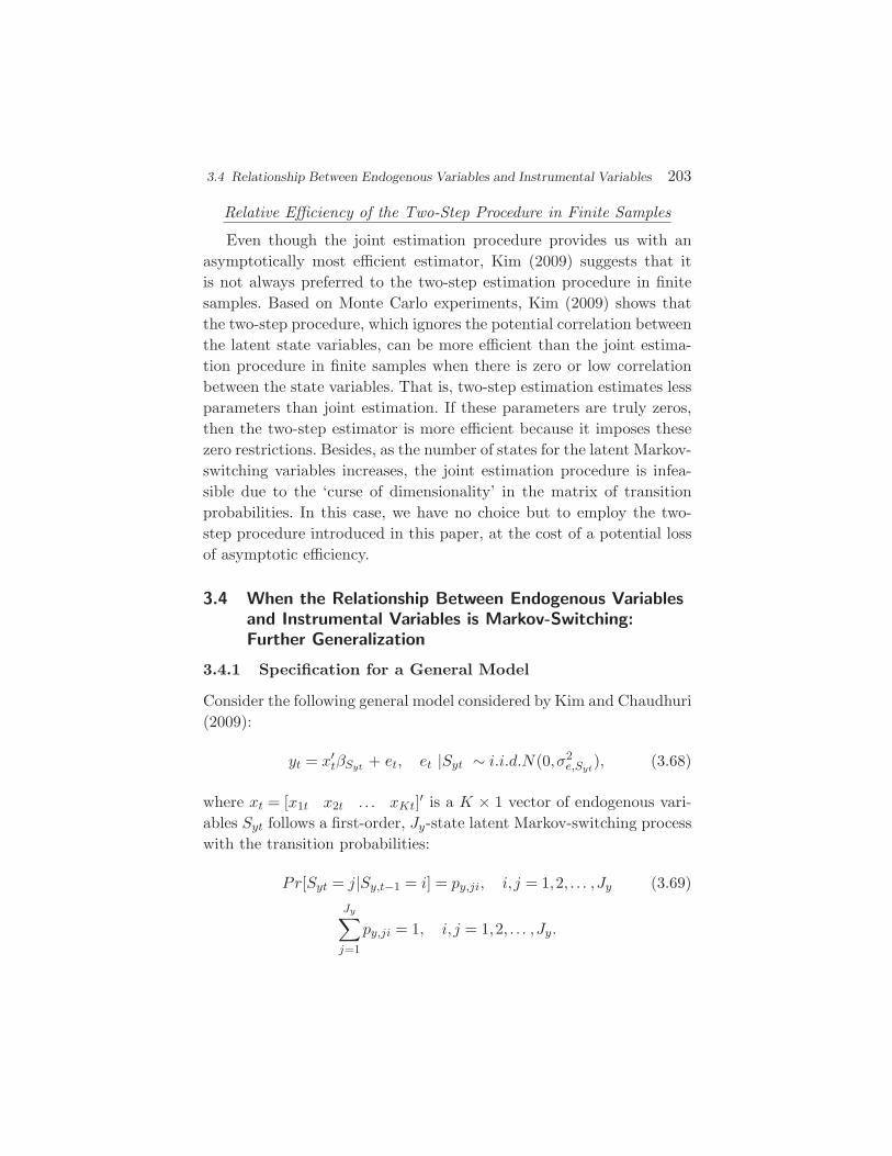
3.4 Relationship Between Endogenous Variables and Instrumental Variables 203
Relative Efficiency of the Two-Step Procedure in Finite Samples
Even though the joint estimation procedure provides us with anasymptotically most efficient estimator, Kim (2009) suggests that itis not always preferred to the two-step estimation procedure in finitesamples. Based on Monte Carlo experiments, Kim (2009) shows thatthe two-step procedure, which ignores the potential correlation betweenthe latent state variables, can be more efficient than the joint estima-tion procedure in finite samples when there is zero or low correlationbetween the state variables. That is, two-step estimation estimates lessparameters than joint estimation. If these parameters are truly zeros,then the two-step estimator is more efficient because it imposes thesezero restrictions. Besides, as the number of states for the latent Markov-switching variables increases, the joint estimation procedure is infea-sible due to the ‘curse of dimensionality’ in the matrix of transitionprobabilities. In this case, we have no choice but to employ the two-step procedure introduced in this paper, at the cost of a potential lossof asymptotic efficiency.
3.4 When the Relationship Between Endogenous Variablesand Instrumental Variables is Markov-Switching:Further Generalization
3.4.1 Specification for a General Model
Consider the following general model considered by Kim and Chaudhuri(2009):
yt = x′tβSyt + et, et |Syt ∼ i.i.d.N(0,σ2
e,Syt), (3.68)
where xt = [x1t x2t . . . xKt]′ is a K × 1 vector of endogenous vari-ables Syt follows a first-order, Jy-state latent Markov-switching processwith the transition probabilities:
Pr[Syt = j|Sy,t−1 = i] = py,ji, i, j = 1,2, . . . ,Jy (3.69)
Jy∑j=1
py,ji = 1, i, j = 1,2, . . . ,Jy.
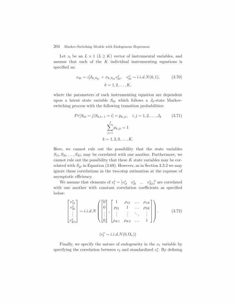
204 Markov-Switching Models with Endogenous Regressors
Let zt be an L × 1 (L ≥ K) vector of instrumental variables, andassume that each of the K individual instrumenting equations isspecified as:
xkt = z′tδk,Skt
+ σk,Sktv∗kt, v∗
kt ∼ i.i.d.N(0,1), (3.70)
k = 1,2, . . . ,K,
where the parameters of each instrumenting equation are dependentupon a latent state variable Skt which follows a Jk-state Markov-switching process with the following transition probabilities:
Pr[Skt = j|Sk,t−1 = i] = pk,ji, i, j = 1,2, . . . ,Jk (3.71)
J∑j=1
pk,ji = 1
k = 1,2,3, . . . ,K.
Here, we cannot rule out the possibility that the state variablesS1t,S2t, . . . ,SKt may be correlated with one another. Furthermore, wecannot rule out the possibility that these K state variables may be cor-related with Syt in Equation (3.69). However, as in Section 3.3.2 we mayignore these correlations in the two-step estimation at the expense ofasymptotic efficiency.
We assume that elements of v∗t = [v∗
1t v∗2t ... v∗
Kt]′ are correlated
with one another with constant correlation coefficients as specifiedbelow:
v∗1t
v∗2t...v∗Kt
∼ i.i.d.N
00...0
,
1 ρ12 . . . ρ1K
ρ21 1 . . . ρ2K...
.... . .
...ρK1 ρK2 . . . 1
. (3.72)
(v∗t ∼ i.i.d.N(0,Ωv))
Finally, we specify the nature of endogeneity in the xt variable byspecifying the correlation between et and standardized v∗
t . By defining
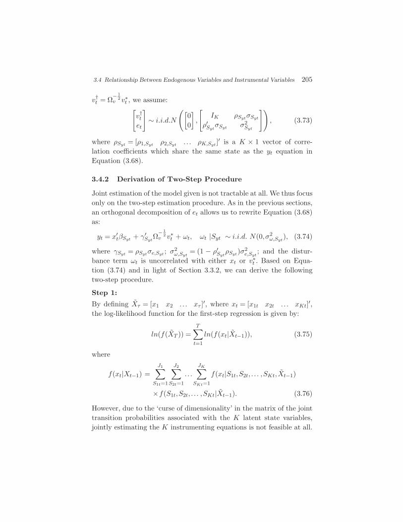
3.4 Relationship Between Endogenous Variables and Instrumental Variables 205
v†t = Ω
− 12
v v∗t , we assume:[
v†t
et
]∼ i.i.d.N
([00
],
[IK ρSytσSyt
ρ′SytσSyt σ2
Syt
]), (3.73)
where ρSyt = [ρ1,Syt ρ2,Syt . . . ρK,Syt ]′ is a K × 1 vector of corre-
lation coefficients which share the same state as the yt equation inEquation (3.68).
3.4.2 Derivation of Two-Step Procedure
Joint estimation of the model given is not tractable at all. We thus focusonly on the two-step estimation procedure. As in the previous sections,an orthogonal decomposition of et allows us to rewrite Equation (3.68)as:
yt = x′tβSyt + γ′
SytΩ
− 12
v v∗t + ωt, ωt |Syt ∼ i.i.d. N(0,σ2
ω,Syt), (3.74)
where γSyt = ρSytσe,Syt ; σ2ω,Syt
= (1 − ρ′SytρSyt)σ2
e,Syt; and the distur-
bance term ωt is uncorrelated with either xt or v∗t . Based on Equa-
tion (3.74) and in light of Section 3.3.2, we can derive the followingtwo-step procedure.
Step 1:
By defining Xτ = [x1 x2 . . . xτ ]′, where xt = [x1t x2t . . . xKt]′,the log-likelihood function for the first-step regression is given by:
ln(f(XT )) =T∑
t=1
ln(f(xt|Xt−1)), (3.75)
where
f(xt|Xt−1) =J1∑
S1t=1
J2∑S2t=1
. . .
JK∑SKt=1
f(xt|S1t,S2t, . . . ,SKt, Xt−1)
×f(S1t,S2t, . . . ,SKt|Xt−1). (3.76)
However, due to the ‘curse of dimensionality’ in the matrix of the jointtransition probabilities associated with the K latent state variables,jointly estimating the K instrumenting equations is not feasible at all.
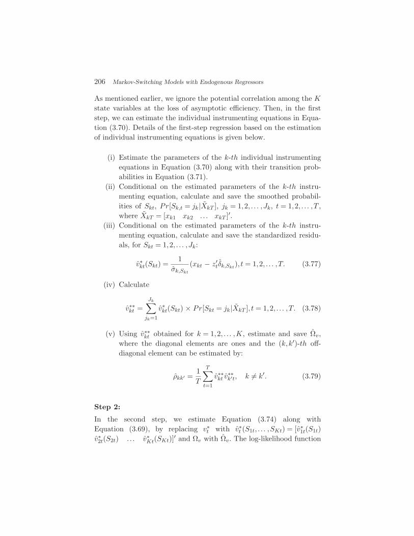
206 Markov-Switching Models with Endogenous Regressors
As mentioned earlier, we ignore the potential correlation among the Kstate variables at the loss of asymptotic efficiency. Then, in the firststep, we can estimate the individual instrumenting equations in Equa-tion (3.70). Details of the first-step regression based on the estimationof individual instrumenting equations is given below.
(i) Estimate the parameters of the k-th individual instrumentingequations in Equation (3.70) along with their transition prob-abilities in Equation (3.71).
(ii) Conditional on the estimated parameters of the k-th instru-menting equation, calculate and save the smoothed probabil-ities of Skt, Pr[Sk,t = jk|XkT ], jk = 1,2, . . . ,Jk, t = 1,2, . . . ,T ,where XkT = [xk1 xk2 . . . xkT ]′.
(iii) Conditional on the estimated parameters of the k-th instru-menting equation, calculate and save the standardized residu-als, for Skt = 1,2, . . . ,Jk:
v∗kt(Skt) =
1σk,Skt
(xkt − z′tδk,Skt
), t = 1,2, . . . ,T. (3.77)
(iv) Calculate
v∗∗kt =
Jk∑jk=1
v∗kt(Skt) × Pr[Skt = jk|XkT ], t = 1,2, . . . ,T. (3.78)
(v) Using v∗∗kt obtained for k = 1,2, . . . ,K, estimate and save Ωv,
where the diagonal elements are ones and the (k,k′)-th off-diagonal element can be estimated by:
ρkk′ =1T
T∑t=1
v∗∗kt v
∗∗k′t, k = k′. (3.79)
Step 2:
In the second step, we estimate Equation (3.74) along withEquation (3.69), by replacing v∗
t with v∗t (S1t, . . . ,SKt) = [v∗
1t(S1t)v∗2t(S2t) . . . v∗
Kt(SKt)]′ and Ωv with Ωv. The log-likelihood function
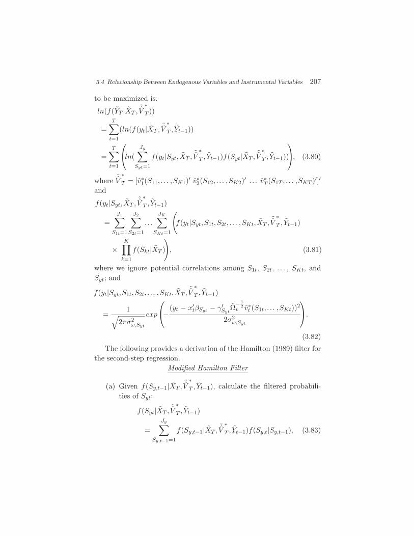
3.4 Relationship Between Endogenous Variables and Instrumental Variables 207
to be maximized is:
ln(f(YT |XT ,˜V
∗T ))
=T∑
t=1
(ln(f(yt|XT ,˜V
∗T , Yt−1))
=T∑
t=1
ln(
Jy∑Syt=1
f(yt|Syt, XT ,˜V
∗T , Yt−1)f(Syt|XT ,
˜V
∗T , Yt−1))
, (3.80)
where ˜V
∗T = [v∗
1(S11, . . . ,SK1)′ v∗2(S12, . . . ,SK2)′ . . . v∗
T (S1T , . . . ,SKT )′]′
and
f(yt|Syt, XT ,˜V
∗T , Yt−1)
=J1∑
S1t=1
J2∑S2t=1
. . .
JK∑SKt=1
(f(yt|Syt,S1t,S2t, . . . ,SKt, XT ,
˜V
∗T , Yt−1)
×K∏
k=1
f(Skt|XT )
), (3.81)
where we ignore potential correlations among S1t, S2t, . . . , SKt, andSyt; and
f(yt|Syt,S1t,S2t, . . . ,SKt, XT ,˜V
∗T , Yt−1)
=1√
2πσ2ω,Syt
exp
−
(yt − x′tβSyt − γ′
SytΩ
− 12
v v∗t (S1t, . . . ,SKt))2
2σ2w,Syt
.(3.82)
The following provides a derivation of the Hamilton (1989) filter forthe second-step regression.
Modified Hamilton Filter
(a) Given f(Sy,t−1|XT ,˜V
∗T , Yt−1), calculate the filtered probabili-
ties of Syt:
f(Syt|XT ,˜V
∗T , Yt−1)
=Jy∑
Sy,t−1=1
f(Sy,t−1|XT ,˜V
∗T , Yt−1)f(Sy,t|Sy,t−1), (3.83)
208 Markov-Switching Models with Endogenous Regressors
Syt = 1,2, . . . ,Jy,
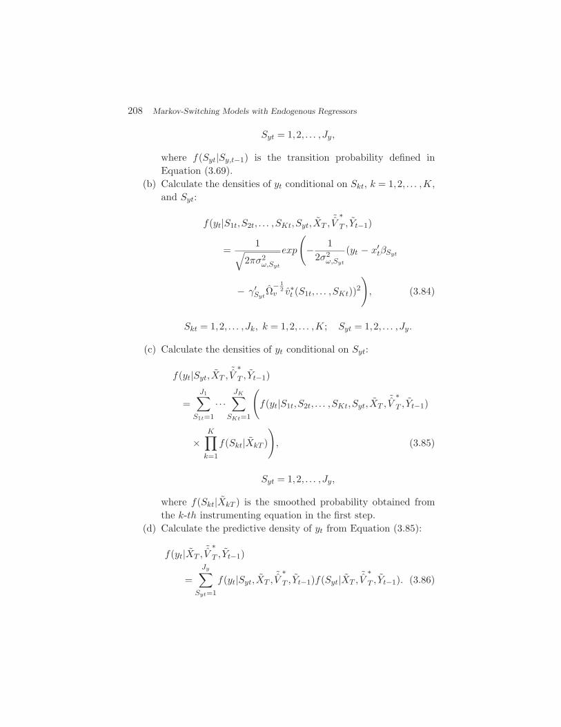
where f(Syt|Sy,t−1) is the transition probability defined inEquation (3.69).
(b) Calculate the densities of yt conditional on Skt, k = 1,2, . . . ,K,and Syt:
f(yt|S1t,S2t, . . . ,SKt,Syt, XT ,˜V
∗T , Yt−1)
=1√
2πσ2ω,Syt
exp
(− 1
2σ2ω,Syt
(yt − x′tβSyt
− γ′Syt
Ω− 1
2v v∗
t (S1t, . . . ,SKt))2), (3.84)
Skt = 1,2, . . . ,Jk, k = 1,2, . . . ,K; Syt = 1,2, . . . ,Jy.
(c) Calculate the densities of yt conditional on Syt:
f(yt|Syt, XT ,˜V
∗T , Yt−1)
=J1∑
S1t=1
· · ·JK∑
SKt=1
(f(yt|S1t,S2t, . . . ,SKt,Syt, XT ,
˜V
∗T , Yt−1)
×K∏
k=1
f(Skt|XkT )
), (3.85)
Syt = 1,2, . . . ,Jy,
where f(Skt|XkT ) is the smoothed probability obtained fromthe k-th instrumenting equation in the first step.
(d) Calculate the predictive density of yt from Equation (3.85):
f(yt|XT ,˜V
∗T , Yt−1)
=Jy∑
Syt=1
f(yt|Syt, XT ,˜V
∗T , Yt−1)f(Syt|XT ,
˜V
∗T , Yt−1). (3.86)
3.5 Backward-Looking Component Important 209
(e) Calculate the updated probabilities of Syt:
f(Syt|XT ,˜V
∗T , Yt) =
f(yt|Syt, XT ,˜V
∗T , Yt−1)f(Syt|XT ,
˜V
∗T , Yt−1)
f(yt|XT ,˜V
∗T , Yt−1)
.
(3.87)
(f) Using Equation (3.86), calculate
lnLy = lnLy + ln(f(yt|XT ,˜V
∗T , Yt−1)). (3.88)
Starting with the unconditional probabilities (f(Sy,0)) and lnly = 0,we can iterate the above algorithm for t = 1,2, . . . ,T to evaluate the log-likelihood value defined in Equation (3.80). Conditional on the esti-mated parameters, Equations (3.83) and (3.88) provide us with thefiltered probabilities of Syt.
Addressing the Problem of Generated RegressorsThe procedure for correcting for the standard errors of the coeffi-
cient estimates from the second step is the same as in Section 3.1.2.
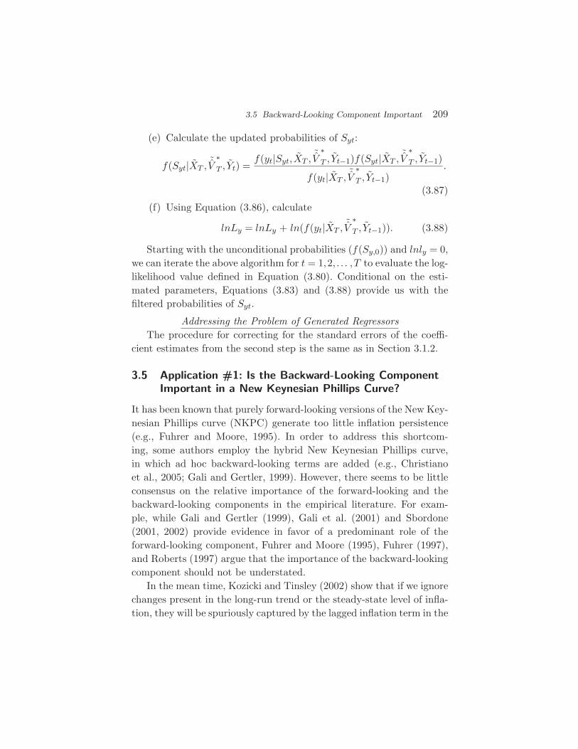
3.5 Application #1: Is the Backward-Looking ComponentImportant in a New Keynesian Phillips Curve?
It has been known that purely forward-looking versions of the New Key-nesian Phillips curve (NKPC) generate too little inflation persistence(e.g., Fuhrer and Moore, 1995). In order to address this shortcom-ing, some authors employ the hybrid New Keynesian Phillips curve,in which ad hoc backward-looking terms are added (e.g., Christianoet al., 2005; Gali and Gertler, 1999). However, there seems to be littleconsensus on the relative importance of the forward-looking and thebackward-looking components in the empirical literature. For exam-ple, while Gali and Gertler (1999), Gali et al. (2001) and Sbordone(2001, 2002) provide evidence in favor of a predominant role of theforward-looking component, Fuhrer and Moore (1995), Fuhrer (1997),and Roberts (1997) argue that the importance of the backward-lookingcomponent should not be understated.
In the mean time, Kozicki and Tinsley (2002) show that if we ignorechanges present in the long-run trend or the steady-state level of infla-tion, they will be spuriously captured by the lagged inflation term in the
210 Markov-Switching Models with Endogenous Regressors
hybrid NKPC specification. Furthermore, in a recent paper, Cogley andSbordone (2008) derive a version of the NKPC that incorporates a time-varying long-run trend component of inflation, which they attribute toshifts in monetary policy. They show that when drift in trend infla-tion is taken into account, a pure NKPC with only a forward-lookingcomponent fits the data well.
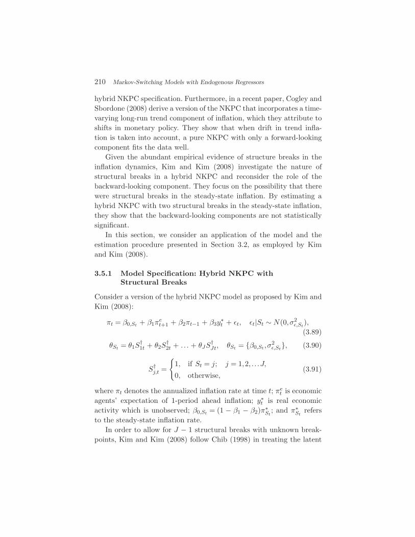
Given the abundant empirical evidence of structure breaks in theinflation dynamics, Kim and Kim (2008) investigate the nature ofstructural breaks in a hybrid NKPC and reconsider the role of thebackward-looking component. They focus on the possibility that therewere structural breaks in the steady-state inflation. By estimating ahybrid NKPC with two structural breaks in the steady-state inflation,they show that the backward-looking components are not statisticallysignificant.
In this section, we consider an application of the model and theestimation procedure presented in Section 3.2, as employed by Kimand Kim (2008).
3.5.1 Model Specification: Hybrid NKPC withStructural Breaks
Consider a version of the hybrid NKPC model as proposed by Kim andKim (2008):
πt = β0,St + β1πet+1 + β2πt−1 + β3y
∗t + εt, εt|St ∼ N(0,σ2
ε,St),(3.89)
θSt = θ1S†1t + θ2S
†2t + . . . + θJS
†Jt, θSt = β0,St ,σ
2ε,St
, (3.90)
S†j,t =
1, if St = j; j = 1,2, . . .J,
0, otherwise,(3.91)
where πt denotes the annualized inflation rate at time t; πet is economic
agents’ expectation of 1-period ahead inflation; y∗t is real economic
activity which is unobserved; β0,St = (1 − β1 − β2)π∗St
; and π∗St
refersto the steady-state inflation rate.
In order to allow for J − 1 structural breaks with unknown break-points, Kim and Kim (2008) follow Chib (1998) in treating the latent
3.5 Backward-Looking Component Important 211
state variable (St) as a first-order Markov-switching process with non-recurring states. Thus, the matrix of the transition probabilities isgiven by:
P =
p11 0 . . . 0 01 − p11 p22 . . . 0 0
0 1 − p22 . . . 0 0...
.... . .
......
0 0 . . . pJ−1,J−1 00 0 . . . 1 − pJ−1,J−1 1
, (3.92)
where pj,j = Pr[St = j|St−1 = j] and j = 1,2, . . . ,J . The probability ofstaying in the terminal state (pJ,J) is set to 1. The expected duration ofregime j (St = j) is calculated by 1
1−pjj. Note that each break point is
estimated to be the sum of the expected durations of past and currentregimes.
Following Roberts (1995, 1997, 1998), Kozicki and Tinsley (2001),Erceg and Levin (2003), Carroll (2003), Adam and Padula (2003), theπe
t+1 term can be proxied by a survey measure of inflation forecasts(πs
t+1). The y∗t term can be proxied by a measure of the output gap
(yt). However, Kim and Kim (2008) consider the possibility that thesurvey measure of inflation (πs
t+1) and a measure of the output gap(yt) may be contaminated by measurement errors. Thus, the followingequation, in which πe
t+1 and y∗t in Equation (3.89) are replaced by πs
t+1and yt, suffers from the errors-in-variables problem:
πt = β0,St + β1πst+1 + β2πt−1 + β3yt + et, et|St ∼ N(0,σ2
e,St), (3.93)
where et = εt + (β1(πet+1 − πs
t+1) + β2(y∗t − yt)) and both πs
t+1 and yt
are correlated with et.In order to deal with the problem of endogeneity in Equation (3.93),
the following instrumenting equations are introduced:
[πs
t+1yt
]=[z′t 00 z′
t
][δ1,St
δ2,St
]+
[σ2
1,Stσ12,St
σ12,St σ22,St
] 12 [v∗1t
v∗2t
], (3.94)
(xt = Z ′tδt + Σ
12v,St
v∗t , v∗
t ∼ i.i.d.N(0, I2))
212 Markov-Switching Models with Endogenous Regressors
[v∗t
et
]∼ N
([00
],
[I2 ρStσe,St
ρ′Stσe,St σ2
e,St
]), (3.95)
where zt is a vector of instrumental variables; ρSt = [ρ1,St ρ2,St ]′ is a
2 × 1 vector of correlation coefficients between v∗t and et. It is assumed
that a common latent state variable St determines the nature of struc-tural breaks in both the NKPC and the instrumenting Equations in(3.93) and (3.94). This allows us to employ the estimation procedureproposed by Kim (2004) and described in Section 3.2, based on thefollowing representation of Equation (3.93):
πt = β0,St + β1πst+1 + β2πt−1 + β3yt + ρ1,Stσe,Stv
∗1,t
+ρ2,Stσe,Stv∗2,t + ωt, (3.96)
ωt|St ∼ N(0,(1 − ρ21,St
− ρ22,St
)σ2e,St
),
which results from an orthogonal decomposition of et in Equa-tion (3.93). Here, conditional on St, the disturbance term ωt is uncor-related with v∗
t in Equation (3.94). This leads to an easy derivation ofthe log-likelihood function for joint estimation of Equations (3.96) and(3.94).
3.5.2 Empirical Results
For inflation data, quarterly gross domestic product (GDP) deflatorinflation and the Survey of Professional Forecasters (SPF) are used asin Kim and Kim (2008). As a proxy for real economic activity, the CBOoutput gap measure is used. Four lags of each of the following variablesare used as instruments: the actual inflation rate, the CBO output gap,the change in the federal funds rate and wage inflation measured bythe growth rate of non-farm business compensation. The sample spans1968:Q4–2006:Q1.
When the model is estimated without allowing for structural breaks,the backward-looking component is statistically significant. Besides, thenull of no serial correlation in the residuals was strongly rejected, sug-gesting a potential model misspecification. Similar results are obtained
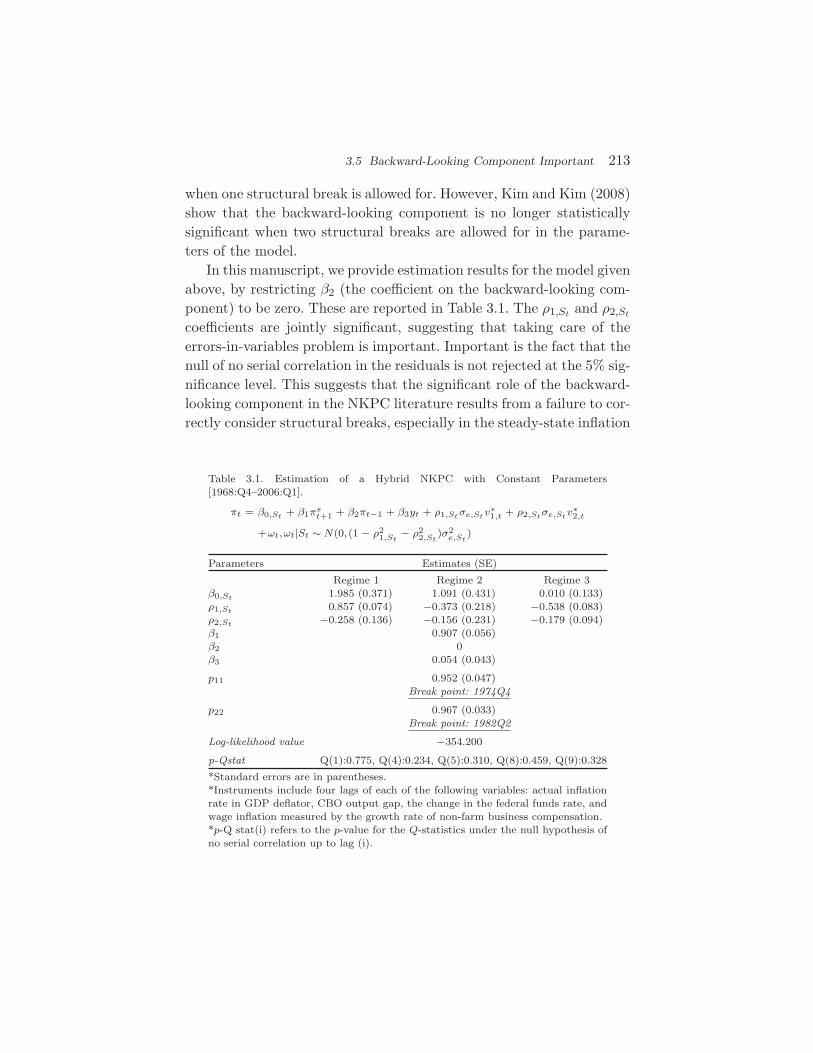
3.5 Backward-Looking Component Important 213
when one structural break is allowed for. However, Kim and Kim (2008)show that the backward-looking component is no longer statisticallysignificant when two structural breaks are allowed for in the parame-ters of the model.
In this manuscript, we provide estimation results for the model givenabove, by restricting β2 (the coefficient on the backward-looking com-ponent) to be zero. These are reported in Table 3.1. The ρ1,St and ρ2,St
coefficients are jointly significant, suggesting that taking care of theerrors-in-variables problem is important. Important is the fact that thenull of no serial correlation in the residuals is not rejected at the 5% sig-nificance level. This suggests that the significant role of the backward-looking component in the NKPC literature results from a failure to cor-rectly consider structural breaks, especially in the steady-state inflation
Table 3.1. Estimation of a Hybrid NKPC with Constant Parameters[1968:Q4–2006:Q1].
πt = β0,St + β1πst+1 + β2πt−1 + β3yt + ρ1,Stσe,Stv∗
1,t + ρ2,Stσe,Stv∗2,t
+ωt,ωt|St ∼ N(0,(1 − ρ21,St
− ρ22,St
)σ2e,St
)
Parameters Estimates (SE)
Regime 1 Regime 2 Regime 3β0,St 1.985 (0.371) 1.091 (0.431) 0.010 (0.133)ρ1,St 0.857 (0.074) −0.373 (0.218) −0.538 (0.083)ρ2,St −0.258 (0.136) −0.156 (0.231) −0.179 (0.094)β1 0.907 (0.056)β2 0β3 0.054 (0.043)
p11 0.952 (0.047)Break point: 1974Q4
p22 0.967 (0.033)Break point: 1982Q2
Log-likelihood value −354.200
p-Qstat Q(1):0.775, Q(4):0.234, Q(5):0.310, Q(8):0.459, Q(9):0.328
*Standard errors are in parentheses.*Instruments include four lags of each of the following variables: actual inflationrate in GDP deflator, CBO output gap, the change in the federal funds rate, andwage inflation measured by the growth rate of non-farm business compensation.*p-Q stat(i) refers to the p-value for the Q-statistics under the null hypothesis ofno serial correlation up to lag (i).
214 Markov-Switching Models with Endogenous Regressors
rate. U.S. inflation dynamics can be explained well by a purely forward-looking version of the NKPC, if we appropriately consider the possibil-ity of structural breaks in the steady-state inflation rate.
3.6 Application #2: The Nature of the Structural Breakin the Excess Sensitivity of Consumption to Income
In this section, we consider an application of the model and the two-step estimation procedure described in Section 3.3. We take an appli-cation from Kim (2009), who allows for a structural break in Campbelland Mankiw’s (1989, 1991) consumption function, in investigating thenature of the structural break in the excess sensitivity of consumptionto income. The model considered is:
∆Ct = µS1t + λS1t∆Yt + et, et|S1t ∼ N(0,σ2e,S1t
), S1t = 1,2,(3.97)
∆Yt = z′tδS2t + σv,S2tv
∗t , vt ∼ i.i.d.N(0,1), S2t = 1,2, (3.98)
[v∗t
et
]∼ N
([00
],
[1 ρS1tσe,S1t
ρS1tσe,S1t σ2e,S1t
]), (3.99)
Pr[S1t = 1|S1,t−1 = 1] = p1,11, P r[S1t = 2|S1,t−1 = 2] = 1, (3.100)
Pr[S2t = 1|S2,t−1 = 1] = p2,11, P r[S2t = 2|S2,t−1 = 2] = 1, (3.101)
where Yt is the log of per-capita disposable personal income; Ct is thelog of per-capita consumption on non-durable goods and services; ρS1t
is the correlation coefficient between v∗t and et; zt is a vector of instru-
mental variables not correlated with et; and λS1t is interpreted as thefraction of aggregate income that accrues to individuals who consumetheir current income (‘rule-of-thumb’ consumers) in the presence ofliquidity constraints.
The transition probabilities in Equations (3.100) and (3.101) implythat one structural break is implemented in both the consumption func-tion and the instrumenting equation in Equations (3.97) and (3.98).Given the transition probabilities p1,11 and p2,11, the break dates for
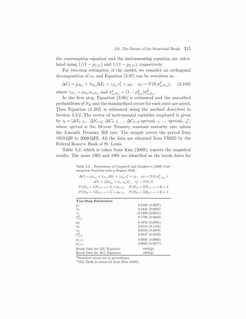
3.6 The Nature of the Structural Break 215
the consumption equation and the instrumenting equation are calcu-lated using 1/(1 − p1,11) and 1/(1 − p2,11), respectively.
For two-step estimation of the model, we consider an orthogonaldecomposition of et, and Equation (3.97) can be rewritten as:
∆Ct = µS1t + λS1t∆Yt + γS1tv∗t + ωt, ωt ∼ N(0,σ2
ω,S1t), (3.102)
where γS1t = ρS1tσe,S1t and σ2ω,S1t
= (1 − ρ2S1t
)σ2e,S1t
.In the first step, Equation (3.98) is estimated and the smoothed
probabilities of S2t and the standardized errors for each state are saved.Then Equation (3.102) is estimated using the method described inSection 3.3.2. The vector of instrumental variables employed is givenby zt = [∆Yt−2 . . .∆Yt−4; ∆Ct−2 . . . ∆Ct−4;spreadt−2 . . . spreadt−4]′,where spread is the 10-year Treasury constant maturity rate minusthe 3-month Treasury Bill rate. The sample covers the period from1953:QII to 2006:QIII. All the data are obtained from FRED by theFederal Reserve Bank of St. Louis.
Table 3.2, which is taken from Kim (2009), reports the empiricalresults. The years 1985 and 1991 are identified as the break dates for
Table 3.2. Estimation of Campbell and Mankiw’s (1989) Con-sumption Function with a Regime Shift.
∆Ct = µS1t + λS1t∆Yt + γS1tv∗t + ωt, ωt ∼ N(0,σ2
ω,S1t)
∆Yt = z′tδS2t
+ σv,S2tv∗
t , v∗t ∼ N(0,1)
Pr[S1t = 1|S1,t−1 = 1] = p1,11, P r[S1t = 2|S1,t−1 = 2] = 1
Pr[S2t = 1|S2,t−1 = 1] = p2,11, P r[S2t = 2|S2,t−1 = 2] = 1
Two-Step Estimationµ1 0.2589 (0.0637)λ1 0.4444 (0.0993)γ1 −0.1469 (0.0861)σ2
ω,1 0.1790 (0.0262)
µ2 0.4452 (0.0591)λ2 0.0134 (0.1122)γ2 0.0559 (0.0859)σ2
ω,2 0.0847 (0.0182)
p1,11 0.9935 (0.0065)p2,11 0.9923 (0.0077)
Break Date for ∆Yt Equation 1985Q4Break Date for ∆Ct Equation 1991Q1
*Standard errors are in parentheses.*This Table is extracted from Kim (2009).
216 Markov-Switching Models with Endogenous Regressors
the income equation and the consumption equation, respectively. Beforethe structural break in the year 1991, the estimate of λ1 is 0.444 andit is statistically significant. After the structural break, however, thisestimate is close to zero and statistically insignificant. Excess sensi-tivity of consumption to disposable income seems to have disappearedsince the mid-1980s. One potential explanation is the deregulation infinancial institutions that started in the mid-1990s, which may haveimproved the credit conditions of the economic agents. However, theregime-shifting nature of the excess sensitivity of consumption to dis-posable income warrants further investigation.
4Markov-Switching Models with Endogenous
Switching: When the State Variable andRegression Disturbance are Correlated
In the microeconometrics literature, switching models with endoge-nous switching have a long history. For example, sample-selection mod-els (Heckman, 1979) and disequilibrium models (Maddala and Nelson,1974, 1975) belong to the general class of switching models with theswitch determined endogenously.1 In these models, a decision processand the regression models with which each decision option is associ-ated are specified. Then, depending on the value of the latent decisionvariable relative to a threshold value, the regime for the observationalunits is determined. Here, we have endogenous switching if the distur-bance terms in the decision process and the regression equations arecorrelated.
In the time-series literature, Markov-switching regression models(Hamilton, 1989) differ from the switching models in that the latentstate variable that determines the regime follows a Markov structure.The vast literature generated by Hamilton (1989) typically assumesthat the regime shifts are exogenous with respect to all realizations of
1 For a survey of these models, readers are referred to Maddala (1983).
217
218 Markov-Switching Models with Endogenous Switching
the regression disturbance. In this section, we deal with an extensionof the Hamilton model to deal with the issue of endogenous switching,as implemented by Kim et al. (2008). While Section 3 deals with theissue of endogenous regressors in the Markov-switching models, thissection deals with the issue of endogenous switching by assuming thatthe regressors are exogenous.
As a motivation for endogenous switching in a macroeconomic orfinance model of Markov-switching, Kim et al. (2008) consider a situa-tion in which economic agents react to the unobserved state of the econ-omy that follows a Markov-switching process. If the economic agentsdraw inferences about the unobserved state based on some informationset, the contents of which are unknown to the econometrician, one hasno choice but to use the actual state as a proxy for this inference in anempirical model. This leads to the problem of errors-in-variables, andthus endogeneity. Examples include the models of equity returns givenin Turner et al. (1989) and Kim et al. (2004). Besides, in many appli-cations of the Markov-switching regression models in macroeconomicsor finance, it may be natural to assume that the state is correlatedwith the regression disturbance. For example, it is often the case thatthe estimated state variable is strongly correlated with the businesscycle. This can be seen in recent applications of the regime-switchingmodel to identified monetary VARs, such as Sims and Zha (2006). Itis not hard to imagine that macroeconomic shocks to the VAR may becorrelated with the business cycle.
4.1 Model Specification
Consider the following Markov-switching regression model:
yt = x′tβSt + σStεt, εt ∼ i.i.d.N(0,1), (4.1)
where yt is 1 × 1 and xt is a K × 1 vector of exogenous or predeter-mined variables. We assume that the latent variable St follows a first-order two-state Markov process and it is correlated with the regressiondisturbance εt. In order to specify the correlation between the discretevariable St and the continuous variable εt, we employ a continuous
4.2 Derivation of the Hamilton Filter and the Log-Likelihood Function 219
latent variable S∗t with the following decision process2:
S∗t = aSt−1 + ηt, ηt ∼ i.i.d.N(0,1), (4.2)
St =
1, if S∗
t ≥ 0 (i.e., if ηt ≥ −aSt−1)
0, if S∗t < 0 (i.e., if ηt < −aSt−1),
(4.3)
which leads to the following probit specification for the transition prob-abilities for St:
Pr(St = 1|St−1 = i) = 1 − Φ(−ai),P r(St = 0|St−1 = i) = Φ(−ai), i = 0,1,
(4.4)
where Φ(.) is the standard normal cumulative distribution function(c.d.f). Here, the correlation between St and εt is specified indirectlythrough the correlation between ηt and εt, in the following joint distri-bution: [
εtηt
]∼ i.i.d.N(0,Σ), Σ =
[1 ρ
ρ 1
], (4.5)
where E(εtηt−h) = 0, for all h = 0.
4.2 Derivation of the Hamilton Filter and theLog-Likelihood Function
The key to a successful estimation of the model is in appropriatelyderiving the density of yt conditional on St, St−1, and xt. For this pur-pose, we consider the following orthogonal decomposition of ηt basedon the Cholesky decomposition of Σ in Equation (4.5):
ηt = ρεt +√
1 − ρ2ωt
= ρ
(yt − x′
tβSt
σSt
)+√
1 − ρ2ωt, ωt ∼ i.i.d.N(0,1), (4.6)
where ωt is uncorrelated with either εt or xt.
2 If the latent variable S∗t is specified as a function of zt, a vector of predetermined or exoge-
nous variables, we have a model with time-varying transition probabilities as consideredby Filardo (1994) and Diebold et al. (1994).
220 Markov-Switching Models with Endogenous Switching
Given Equation (4.6), we first derive f(yt|St = 1,St−1 = st−1,xt).By noting that:
f(yt|St = 1,St−1 = st−1,xt) = f(yt|η ≥ −ast−1 ,xt), (4.7)
we consider the c.d.f.
Pr(yt < g|ηt ≥ −ast−1 ,xt) =Pr(yt < g,ηt ≥ −ast−1 |xt)
1 − Φ(−ast−1)
=Pr
(yt < g,ωt ≥ −ast−1−ρεt√
1−ρ2|xt
)1 − Φ(−ast−1)
(4.8)
where the numerator is
Pr
(yt < g,ωt ≥ −ast−1 − ρεt√
1 − ρ2|xt
)
=∫ g
−∞
∫ ∞−ast−1−ρεt√
1−ρ2
f(yt,ωt|xt)dωtdεt
=∫ g
−∞
∫ ∞−ast−1−ρεt√
1−ρ2
f(yt|xt)f(ωt|xt)dωtdεt
=∫ g
−∞1σ1φ
(yt − x′
tβ1
σ1
)(1 − Φ
(−ast−1 − ρ(yt − x′
tβ1)/σ1√1 − ρ2
))dεt,
(4.9)
where φ(.) is the standard normal probability density function. By sub-stituting Equation (4.9) into Equation (4.8), and differentiating it withrespect to εt, we have:
f(yt|St = 1,St−1 = st−1,xt)
=1σ1φ
(yt − x′
tβ1
σ1
)
×(1 − Φ
(−ast−1 − ρ(yt − x′
tβ1)/σ1√1 − ρ2
))/(1 − Φ(−ast−1)
), (4.10)
st−1 = 0,1.
4.2 Derivation of the Hamilton Filter and the Log-Likelihood Function 221
In exactly the same way, we can derive:
f(yt|St = 0,St−1 = st−1,xt)
=1σ0φ
(yt − x′
tβ0
σ0
)Φ
(−ast−1 − ρ(yt − x′
tβ0)/σ0√1 − ρ2
)/Φ(−ast−1
),
(4.11)
st−1 = 0,1.
In the case of exogenous switching (ρ = 0), Equations (4.10) and(4.11) collapse to:
f(yt|St = st,St−1 = st−1,xt) =1σst
φ
(yt − x′
tβst
σst
), st,st−1 = 0,1,
(4.12)
which suggests that yt follows a conditional normal distribution. In thecase of endogenous switching (ρ = 0), however, Equations (4.10) and(4.11) suggest that yt is not normally distributed conditional on St,St−1, and xt. Furthermore, we note that
E(εt|St = 1,St−1 = st−1,xt) = E(εt|ηt ≥ −ast−1)
= ρφ(−ast−1)
1 − Φ(−ast−1)= 0, (4.13)
E(εt|St = 0,St−1 = st−1,xt) = E(εt|ηt < −ast−1)
= −ρ φ(−ast−1)Φ(−ast−1)
= 0, (4.14)
and
V ar(εt|St,St−1,xt) = 1. (4.15)
Thus, in the case of endogenous switching, the usual application of theHamilton filter and the maximum likelihood estimation based on theconditional normality assumption would result in bias in the parameterestimates.
Given the above conditional densities of yt, and by definingXτ = [x1 x2 . . . xτ ]′ and Yτ = [y1 y2 . . . yτ ]′, the log-likelihood
222 Markov-Switching Models with Endogenous Switching
function to be maximized for estimation of the model is given by:
lnL = ln(f(YT |XT ))
=T∑
t=1
ln(f(yt|Xt, Yt−1))
=T∑
t=1
ln
1∑
St=0
1∑St−1=0
f(yt|St,St−1,xt)f(St,St−1|Xt−1, Yt−1)
,(4.16)
where the f(St,St−1|Xt−1, Yt−1) term is obtained from the followingHamilton filter:
Hamilton Filter
(a) For given f(St−1|Yt−1, Xt−1), calculate f(St,St−1|Xt−1, Yt−1)by:
f(St,St−1|Xt−1, Yt−1) = f(St|St−1)f(St−1|Xt−1, Yt−1), (4.17)
where f(St|St−1) is the transition probability specified in Equa-tion (4.4).
(b) Evaluate f(yt|Xt, Yt−1) by:
f(yt|Xt, Yt−1) =1∑
St=0
1∑St−1=0
f(yt|St,St−1,xt)f(St,St−1|Xt−1, Yt−1),
(4.18)
where f(yt|St,St−1,xt) is derived earlier.(c) Calculate f(St,St−1|Xt, Yt) by:
f(St,St−1|Xt, Yt) = f(St,St−1|Xt−1, Yt−1,xt,yt)
=f(yt|St,St−1,xt)f(St,St−1|Xt−1, Yt−1)
f(yt|Xt, Yt−1).
(4.19)
4.3 An Example in Finance: A Volatility FeedbackModel of Stock Returns
Volatility feedback in stock markets is the idea that, in response tonews about dividends in the form of an unexpected change in market
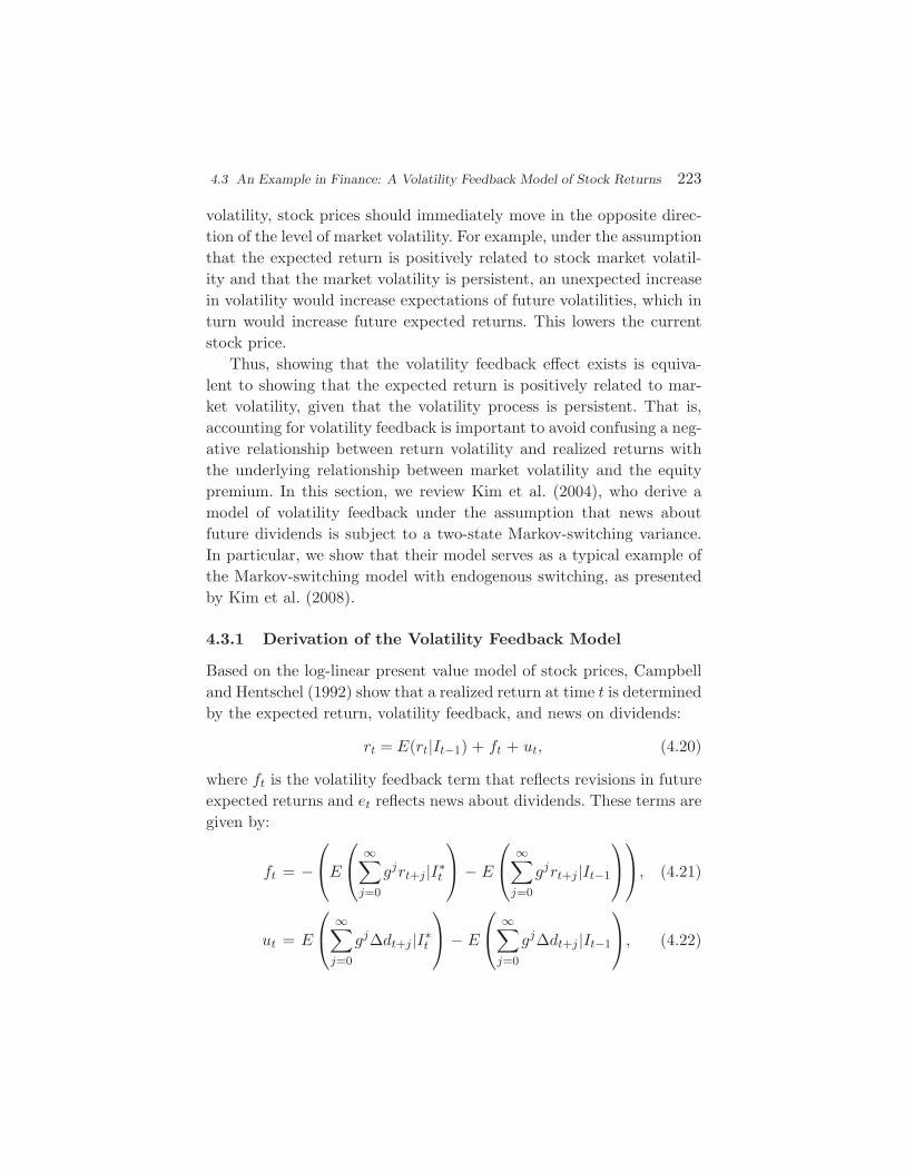
4.3 An Example in Finance: A Volatility Feedback Model of Stock Returns 223
volatility, stock prices should immediately move in the opposite direc-tion of the level of market volatility. For example, under the assumptionthat the expected return is positively related to stock market volatil-ity and that the market volatility is persistent, an unexpected increasein volatility would increase expectations of future volatilities, which inturn would increase future expected returns. This lowers the currentstock price.
Thus, showing that the volatility feedback effect exists is equiva-lent to showing that the expected return is positively related to mar-ket volatility, given that the volatility process is persistent. That is,accounting for volatility feedback is important to avoid confusing a neg-ative relationship between return volatility and realized returns withthe underlying relationship between market volatility and the equitypremium. In this section, we review Kim et al. (2004), who derive amodel of volatility feedback under the assumption that news aboutfuture dividends is subject to a two-state Markov-switching variance.In particular, we show that their model serves as a typical example ofthe Markov-switching model with endogenous switching, as presentedby Kim et al. (2008).
4.3.1 Derivation of the Volatility Feedback Model
Based on the log-linear present value model of stock prices, Campbelland Hentschel (1992) show that a realized return at time t is determinedby the expected return, volatility feedback, and news on dividends:
rt = E(rt|It−1) + ft + ut, (4.20)
where ft is the volatility feedback term that reflects revisions in futureexpected returns and et reflects news about dividends. These terms aregiven by:
ft = −E
∞∑
j=0
gjrt+j |I∗t
− E
∞∑
j=0
gjrt+j |It−1
, (4.21)
ut = E
∞∑
j=0
gj∆dt+j |I∗t
− E
∞∑
j=0
gj∆dt+j |It−1
, (4.22)
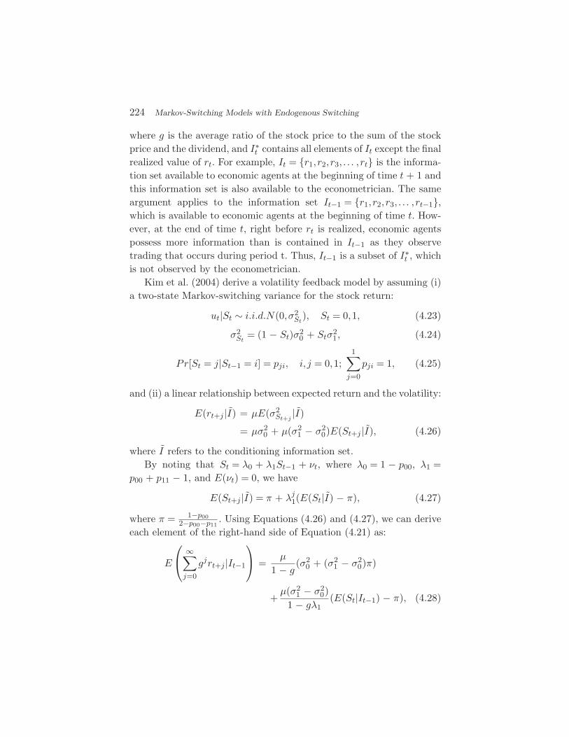
224 Markov-Switching Models with Endogenous Switching
where g is the average ratio of the stock price to the sum of the stockprice and the dividend, and I∗
t contains all elements of It except the finalrealized value of rt. For example, It = r1, r2, r3, . . . , rt is the informa-tion set available to economic agents at the beginning of time t + 1 andthis information set is also available to the econometrician. The sameargument applies to the information set It−1 = r1, r2, r3, . . . , rt−1,which is available to economic agents at the beginning of time t. How-ever, at the end of time t, right before rt is realized, economic agentspossess more information than is contained in It−1 as they observetrading that occurs during period t. Thus, It−1 is a subset of I∗
t , whichis not observed by the econometrician.
Kim et al. (2004) derive a volatility feedback model by assuming (i)a two-state Markov-switching variance for the stock return:
ut|St ∼ i.i.d.N(0,σ2St
), St = 0,1, (4.23)
σ2St
= (1 − St)σ20 + Stσ
21, (4.24)
Pr[St = j|St−1 = i] = pji, i, j = 0,1;1∑
j=0
pji = 1, (4.25)
and (ii) a linear relationship between expected return and the volatility:
E(rt+j |I) = µE(σ2St+j
|I)= µσ2
0 + µ(σ21 − σ2
0)E(St+j |I), (4.26)
where I refers to the conditioning information set.By noting that St = λ0 + λ1St−1 + νt, where λ0 = 1 − p00, λ1 =
p00 + p11 − 1, and E(νt) = 0, we have
E(St+j |I) = π + λj1(E(St|I) − π), (4.27)
where π = 1−p002−p00−p11
. Using Equations (4.26) and (4.27), we can deriveeach element of the right-hand side of Equation (4.21) as:
E
∞∑
j=0
gjrt+j |It−1
=
µ
1 − g(σ2
0 + (σ21 − σ2
0)π)
+µ(σ2
1 − σ20)
1 − gλ1(E(St|It−1) − π), (4.28)
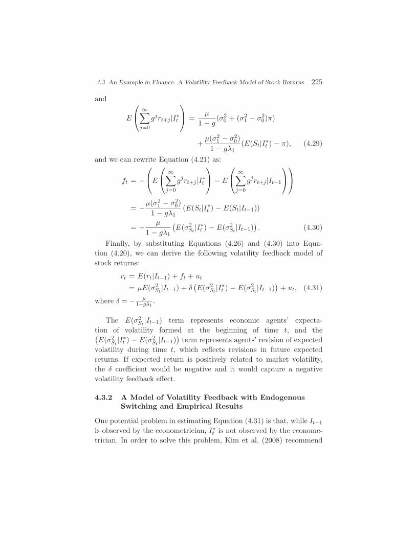
4.3 An Example in Finance: A Volatility Feedback Model of Stock Returns 225
and
E
∞∑
j=0
gjrt+j |I∗t
=
µ
1 − g(σ2
0 + (σ21 − σ2
0)π)
+µ(σ2
1 − σ20)
1 − gλ1(E(St|I∗
t ) − π), (4.29)
and we can rewrite Equation (4.21) as:
ft = −E
∞∑
j=0
gjrt+j |I∗t
− E
∞∑
j=0
gjrt+j |It−1
= −µ(σ21 − σ2
0)1 − gλ1
(E(St|I∗t ) − E(St|It−1))
= − µ
1 − gλ1
(E(σ2
St|I∗
t ) − E(σ2St
|It−1)). (4.30)
Finally, by substituting Equations (4.26) and (4.30) into Equa-tion (4.20), we can derive the following volatility feedback model ofstock returns:
rt = E(rt|It−1) + ft + ut
= µE(σ2St
|It−1) + δ(E(σ2
St|I∗
t ) − E(σ2St
|It−1))
+ ut, (4.31)
where δ = − µ1−gλ1
.
The E(σ2St
|It−1) term represents economic agents’ expecta-tion of volatility formed at the beginning of time t, and the(E(σ2
St|I∗
t ) − E(σ2St
|It−1))
term represents agents’ revision of expectedvolatility during time t, which reflects revisions in future expectedreturns. If expected return is positively related to market volatility,the δ coefficient would be negative and it would capture a negativevolatility feedback effect.
4.3.2 A Model of Volatility Feedback with EndogenousSwitching and Empirical Results
One potential problem in estimating Equation (4.31) is that, while It−1
is observed by the econometrician, I∗t is not observed by the econome-
trician. In order to solve this problem, Kim et al. (2008) recommend
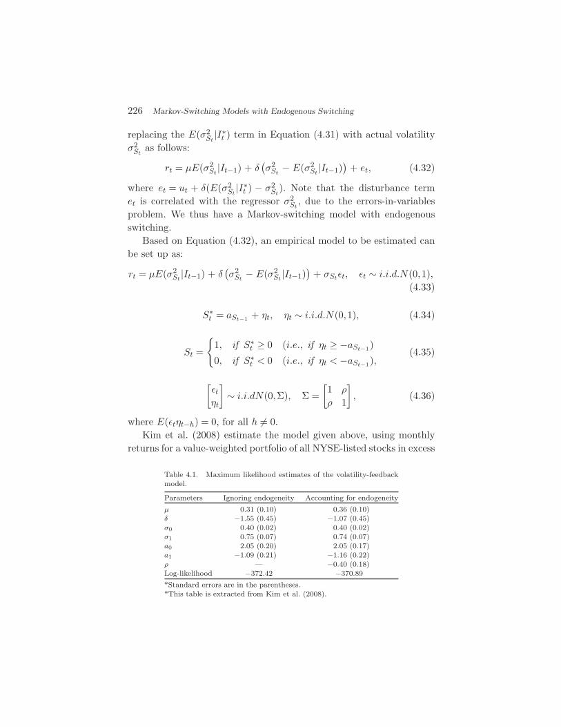
226 Markov-Switching Models with Endogenous Switching
replacing the E(σ2St
|I∗t ) term in Equation (4.31) with actual volatility
σ2St
as follows:
rt = µE(σ2St
|It−1) + δ(σ2
St− E(σ2
St|It−1)
)+ et, (4.32)
where et = ut + δ(E(σ2St
|I∗t ) − σ2
St). Note that the disturbance term
et is correlated with the regressor σ2St
, due to the errors-in-variablesproblem. We thus have a Markov-switching model with endogenousswitching.
Based on Equation (4.32), an empirical model to be estimated canbe set up as:
rt = µE(σ2St
|It−1) + δ(σ2
St− E(σ2
St|It−1)
)+ σStεt, εt ∼ i.i.d.N(0,1),
(4.33)
S∗t = aSt−1 + ηt, ηt ∼ i.i.d.N(0,1), (4.34)
St =
1, if S∗
t ≥ 0 (i.e., if ηt ≥ −aSt−1)
0, if S∗t < 0 (i.e., if ηt < −aSt−1),
(4.35)
[εtηt
]∼ i.i.dN(0,Σ), Σ =
[1 ρ
ρ 1
], (4.36)
where E(εtηt−h) = 0, for all h = 0.Kim et al. (2008) estimate the model given above, using monthly
returns for a value-weighted portfolio of all NYSE-listed stocks in excess
Table 4.1. Maximum likelihood estimates of the volatility-feedbackmodel.
Parameters Ignoring endogeneity Accounting for endogeneity
µ 0.31 (0.10) 0.36 (0.10)δ −1.55 (0.45) −1.07 (0.45)σ0 0.40 (0.02) 0.40 (0.02)σ1 0.75 (0.07) 0.74 (0.07)a0 2.05 (0.20) 2.05 (0.17)a1 −1.09 (0.21) −1.16 (0.22)ρ — −0.40 (0.18)Log-likelihood −372.42 −370.89
*Standard errors are in the parentheses.*This table is extracted from Kim et al. (2008).
4.3 An Example in Finance: A Volatility Feedback Model of Stock Returns 227
of the one-month Treasury Bill rate over the sample period January1952 to December 1999, the same data as used in Kim et al. (2004).Table 4.1, which is taken from Kim et al. (2008), summarizes the results.The first panel shows estimates when endogeneity is ignored (ρ = 0),and the second panel shows estimates when endogeneity is allowed(ρ = 0). In both cases, the µ coefficients are positive and significant andthe δ coefficients are negative and significant. These results are consis-tent with both a positive relationship between the risk premium andexpected future volatility and a substantial volatility feedback effect.The primary difference in the parameter estimates is for the volatilityfeedback coefficient, which is estimated to be about one-third smallerwhen endogeneity is allowed than when it is ignored. Ignoring endoge-nous switching tends to overstate the volatility feedback effect.
5Time-Varying Parameter Models with
Endogenous Regressors
The time-varying parameter models, since their first introduction inthe economics literature in the early 1970s, have been widely used inmodeling instability in economic relations. Literature on time-varyingparameter models in their earlier stage includes Rosenberg (1973), Coo-ley and Prescott (1973, 1976), Belsley (1973), Sarris (1973), etc. Morerecent literature includes Chow (1984), Engle and Watson (1987), andHarvey (1981, 1991). With a growing body of recent empirical evidenceon widespread instability in macroeconomic relations (Stock and Wat-son, 1998), these models have become even more important in appliedmacroeconomics.
Harvey, in his 1981 book and a series of earlier papers, introduced toeconomists the use of the Kalman (1960) filter. It is used for obtainingmaximum likelihood estimates of the hyper-parameters of the state-space models and the time-varying parameter models through pre-diction error decomposition. However, a successful application of theKalman filter to the time-varying parameter models critically dependsupon the assumption that the regressors are either predetermined orexogenous.
228
229
The main purpose of this section is to review recent literature thatdeals with the problem of endogeneity in the time-varying parametermodels. The model we deal with can be considered as a subset of thesimultaneous equations model that consists of K + 1 endogenous vari-ables, as given below:
[yt x′t]Bt = z′
tAt + E′t, Et ∼ i.i.d.N(0,Ω), (5.1)
where yt is 1 × 1; xt is K × 1; [yt x′t]
′ is a vector of (K + 1) × 1endogenous variables; zt is an L × 1 vector of exogenous or predeter-mined variables; Et is a (K + 1) × 1 vector of structural shocks; andBt and At are matrices of time-varying structural coefficients of dimen-sions (K + 1) × (K + 1) and L × (K + 1), respectively. The diagonalelements of Bt are ones. The reduced-form for the above structuralmodel is: [
yt x′t
]= z′
tδt + V ′t , Vt ∼ N(0,Σt), (5.2)
where δt = AtB−1t ; V ′
t = E′tB
−1t ; Σt = B−1′
t ΩB−1t . Here, when the ele-
ments of zt are the lags of the endogenous variables yt and xt, by rear-ranging the reduced-form Equation (5.2) we get a time-varying vec-tor autoregressive (VAR) model which has been recently introducedin the literature (e.g., Cogley and Sargent, 2002; Primiceri, 2005). Inthe literature, the reduced-form VAR model of Equation (5.2) is firstestimated by approximating elements of δt by random walk processes.Then, inferences about the structural coefficients in Equation (5.1) aremade indirectly.
In this section, instead of attempting to estimate the whole systemof simultaneous equations in Equation (5.1), we focus on the estimationof a single equation of interest. For example, given that the first columnof At is an L × 1 vector of zeros, by collecting the first columns of bothsides of Equation (5.1) we get:
yt = x′tβt + et, (5.3)
where βt is the last K × 1 elements of the first column in −Bt and et isthe first element of E′
t. Furthermore, the last K columns of both sidesof the reduced-form VAR in Equation (5.2) can be rearranged to get
230 Time-Varying Parameter Models with Endogenous Regressors
the following seemingly unrelated regression equations (SURE) form:
xt = Z ′tδt + vt, (5.4)
where Z ′t = IK ⊗ z′
t; δt is KL × 1; and vt is last K rows of Vt. Here ztserves as a vector of instrumental variables, and Equation (5.4) is theinstrumenting equation.
We provide a unified framework for dealing with the problem ofendogeneity in the time-varying parameter models of the type in Equa-tion (5.3), as developed by Kim (2006), Kim and Nelson (2006), andKim and Kim (2009). Our main focus is on the two-step estimationof the model. The conventional two-step approach is invalid, as in theMarkov-switching models. We provide two-step estimation proceduresbased on the control function approach, and show how the problem ofgenerated regressors can be taken care of in the second-step regression.
5.1 When the Relation Between the Endogenous Variablesand Instrumental Variables is Time-Invariant
We start our discussion with the following basic model considered byKim (2006)1:
yt = x′tβt + et, (5.5)
βt = βt−1 + εt, εt ∼ i.i.d.N(0,Qy), (5.6)
xt = Z ′tδ + Σ
12v v
∗t , v∗
t ∼ i.i.d.N(0, IK), (5.7)
[v∗t
et
]∼ i.i.d.N
([00
],
[IK×1 ρσe
ρ′σe σ2e
]), (5.8)
where yt is 1 × 1; xt is a K × 1 vector of endogenous regressors cor-related with et; Zt = IK ⊗ zt, with zt being an L × 1 (L ≥ K) vectorof instrumental variables not correlated with et; ρ = [ρ1 ρ2 . . . ρK ]′
1 For simplicity of exposition, we assume that all the regressors in the time-varying parame-ter models in Section 5 are endogenous. It would be straightforward to extend the modelsand the estimation methods to deal with the cases in which only a subset of the regressorsare endogenous.
5.1 Relation Between the Endogenous Variables 231
is a K × 1 vector of correlation coefficients; and εt is not correlatedwith either et or v∗
t . Note that the coefficients of Equation (5.7) aretime-invariant.
For the derivation of a joint estimation and a two-step estimationprocedure, we consider the following representation of Equation (5.5)based on the orthogonal decomposition of et:
yt = x′tβt + γ′v∗
t + ωt, ωt ∼ i.i.d.N(0,σ2ω), (5.9)
where γ = ρσe, σ2ω = (1 − ρ′ρ)σ2
e , v∗t = Σ
− 12
v (xt − Z ′tδ), and ωt is uncor-
related with either xt or v∗t .
5.1.1 Joint Estimation Procedure
The key to the joint estimation procedure is to derive the log-likelihoodfunction for Equations (5.9) and (5.7). It can be derived as:
lnL = ln(f(YT , XT ))
=T∑
t=1
ln(f(yt,xt|Xt−1, Yt−1))
=T∑
t=1
ln(f(xt|Xt−1)f(yt|Xt, Yt−1)), (5.10)
where Xτ = [x1 x2 . . . xτ ]′, Yτ = [y1 y2 . . . yτ ]′, and
f(xt|Xt−1) = (2π)− K2 |Σv|− 1
2 exp
(−1
2(xt − Z ′
tδ)′Σ−1
v (xt − Z ′tδ)),
(5.11)
f(yt|xt, Xt−1, Yt−1) =1√
2πfJt|t−1
exp
(−
(yt − yJt|t−1)
2
2fJt|t−1
), (5.12)
where yJt|t−1 and fJ
t|t−1 are the conditional expectation and the condi-tional variance of yt, respectively. Note that the density of xt in Equa-tion (5.11) is derived from Equation (5.7) and the density of yt inEquation (5.12) is derived from Equation (5.9). The terms yJ
t|t−1 and
232 Time-Varying Parameter Models with Endogenous Regressors
fJt|t−1 can be obtained from the following Kalman filter:
βJt|t−1 = βJ
t−1|t−1, (5.13)
P Jt|t−1 = P J
t−1|t−1 + Qy, (5.14)
yJt|t−1 = x′
tβJt|t−1 + γ′v∗
t = x′tβ
Jt|t−1 + γ′Σ
12v (xt − Z ′
tδ), (5.15)
fJt|t−1 = x′
tPJt|t−1xt + σ2
ω, (5.16)
βJt|t = βJ
t|t−1 + P Jt|t−1xt(fJ
t|t−1)−1(yt − yJ
t|t−1), (5.17)
P Jt|t = P J
t|t−1 − P Jt|t−1xt(fJ
t|t−1)−1x′
tPJt|t−1, (5.18)
where βJt|t−1 = E(βt|Xt, Yt−1), P J
t|t−1 = V ar(βt|Xt, Yt−1), yJt|t−1 =
E(yt|Xt, Yt−1), fJt|t−1 = V ar(yt|Xt, Yt−1), βJ
t|t = E(βt|Xt, Yt), and
P Jt|t = V ar(βt|Xt, Yt).
For joint estimation of the model, we maximize the log-likelihoodfunction in Equation (5.10) with respect to all the parameters of themodel.
5.1.2 Two-Step Estimation Procedure
For a two-step estimation procedure, we consider the following likeli-hood function:
lnL = ln(f(YT , XT ))
= ln(f(YT |XT )) + ln(f(XT )),
=T∑
t=1
ln(f(yt|XT , Yt−1)) +T∑
t=1
ln(f(xt|Xt−1)) (5.19)
which suggests that maximizing the joint log-likelihood func-tion is the same as first maximizing the log-likelihood func-tion (ln(f(XT )) =
∑Tt=1 ln(f(xt|Xt−1))) for the xt equation in
Equation (5.7) and then maximizing the log-likelihood function
5.1 Relation Between the Endogenous Variables 233
(ln(f(YT |XT )) =∑T
t=1 ln(f(yt|XT , Yt−1))) for Equation (5.5) or Equa-tion (5.9) conditional on XT and the parameter estimates from the firststep.
The conventional two-step procedure is invalid. In the first step ofthe conventional two-step procedure, one obtains xt = Z ′
tδ from theOLS regression of Equation (5.7). The second-step regression equationis then given by:
yt = x′tβt + u†
t , (5.20)
where u†t = et + (xt − xt)′βt. The problem with this conventional two-
step procedure is that, conditional on xt, βt is correlated with the dis-turbance term u†
t . This creates another source of endogeneity, resultingin bias in the conventional second-step regression.2
In the second-step estimation procedure based on the control func-tion approach, we want to estimate Equation (5.9) by maximizingthe log-likelihood function ln(f(YT |XT )) = ln(
∏Tt=1 f(yt|XT , Yt−1)). In
order to derive the Kalman filter recursion for the second-step regres-sion, we need:
E(yt|XT , Yt−1) = x′tE(βt|XT , Yt−1) + γ′E(v∗
t |XT ), (5.21)
V ar(yt|XT , Yt−1) = x′tV ar(βt|XT , Yt−1)xt + γ′V ar(v∗
t |XT )γ + σ2ω.
(5.22)
For the second-step regression, we replace the E(v∗t |XT , Yt−1) term in
Equation (5.21) by v∗t , the standardized residuals obtained from an
OLS regression of Equation (5.7). This is equivalent to estimating the
following equation conditional on XT and ˜V
∗T = [v∗
1 v∗2 . . . v∗
T ]′:
yt = x′tβt + γ′v∗
t + ut, (5.23)
2 Harvey (1991) considers a model in which Equations (5.5) and (5.6) are replaced by:
yt = αt + x′tβ + et, (5.5′)
αt = αt−1 + εt, εt ∼ i.i.d.N(0,σ2α), (5.6′)
where only the intercept is time-varying. Even though the conventional two-step procedureprovides us with a consistent estimator for β in this case, it is not easy to correct for theproblem of the generated regressors in the second step. However, the control functionapproach introduced in this section provides an easy solution to this problem.
234 Time-Varying Parameter Models with Endogenous Regressors
where ut = ωt + γ′(v∗t − v∗
t ). Note that, conditional on v∗t = v∗
t , the twoconditional moments of yt in Equations (5.21) and (5.22) should bereplaced by:
E(yt|XT ,˜V
∗T , Yt−1) = x′
tE(βt|XT ,˜V
∗T , Yt−1) + γ′v∗
t , (5.21′)
V ar(yt|XT ,˜V
∗T , Yt−1) = x′
tV ar(βt|XT ,˜V
∗T , Yt−1)xt + σ2
ω, (5.22′)
which will be the basis for derivation of the Kalman filter in the secondstep. However, the use of v∗
t in place of v∗t in Equation (5.9) or the use
of v∗t in place of E(v∗
t |XT ) in Equation (5.21) results in the problemof generated regressors, which needs to be addressed. The followingdescribes the details of the two-step estimation procedure.
Step 1:
(i) We estimate Equation (5.7) by OLS, and get residuals vt =[v1t v2t . . . vKt]′, t = 1,2, . . . ,T .
(ii) We estimate Σv by Σv =∑T
t=11T vtv
′t, and get the standardized
residuals, v∗t = Σ
− 12
v vt, t = 1,2, . . . ,T .
Step 2:
(i) We estimate the hyper-parameters of the model given by Equa-
tions (5.23) and (5.6), conditional on XT and ˜V
∗T . The log-
likelihood function to be maximized is:
lnLy =T∑
t=1
ln(f(yt|XT ,˜V
∗T , Yt−1))
=T∑
t=1
ln
(1√
2πft|t−1exp(−(yt − yt|t−1)2
2ft|t−1)
), (5.24)
where yt|t−1 = E(yt|XT ,˜V
∗T , Yt−1) and ft|t−1 = V ar(yt|XT ,
˜V
∗T , Yt−1), which can be obtained from the following Kalman
filter recursion:
Kalman Filter
βt|t−1 = βt−1|t−1, (5.25)
5.1 Relation Between the Endogenous Variables 235
Pt|t−1 = Pt−1|t−1 + Qy, (5.26)
yt|t−1 = x′tβt|t−1 + γ′v∗
t , (5.27)
ft|t−1 = x′tPt|t−1xt + σ2
ω, (5.28)
βt|t = βt|t−1 + Pt|t−1xtf−1t|t−1(yt − yt|t−1), (5.29)
Pt|t = Pt|t−1 − Pt|t−1xtf−1t|t−1x
′tPt|t−1, (5.30)
where βt|t−1 = E(βt|XT ,˜V
∗T , Yt−1), Pt|t−1 = V ar(βt|XT ,
˜V
∗T ,
Yt−1), βt|t = E(βt|XT ,˜V
∗T , Yt), and Pt|t = V ar(βt|XT ,
˜V
∗T , Yt).
(ii) Get filtered inferences about βt
Conditional on the estimated hyper-parameters, we can runthe above Kalman filter again to get the estimates of the βt
coefficients (βt|t−1 and βt|t) in Equations (5.25) and (5.29).However, the conditional variances of βt (Pt|t−1 and Pt|t) inEquations (5.26) and (5.30) from the above Kalman filter suf-fer from the problem of generated regressors. In order to solvethe problem of generated regressors in calculating the condi-tional variances of βt, we consider the variance of yt conditionalon Yt−1 and XT (but not on ˜
V∗T ), given in Equation (5.22).
Note that, as limT→∞V ar(v∗t |XT ) = IK , Equation (5.22) can
be approximated by:
f∗t|t−1 = V ar(yt|XT , Yt−1) = x′
tV ar(βt|XT , Yt−1)xt + γ′γ + σ2ω,
(5.31)
which allows us to derive the following conditional variances ofβt that do not suffer from the problem of generated regressors:
P ∗t|t−1 = P ∗
t−1|t−1 + Qy, (5.32)
f∗t|t−1 = x′
tP∗t|t−1xt + σ2
ω + γ′γ, (5.33)
P ∗t|t = P ∗
t|t−1 − P ∗t|t−1xtf
∗−1t|t−1x
′tP
∗t|t−1, (5.34)
236 Time-Varying Parameter Models with Endogenous Regressors
where P ∗t|t−1 = V ar(βt|XT , Yt−1), f∗
t|t−1 is defined earlier, and
P ∗t|t = V ar(βt|XT , Yt).
Thus, in order to get correct filtered conditional variances ofβt, we iterate Equations (5.32)–(5.34) for t = 1,2, . . . ,T .
(iii) Get smoothed inferences on βt
The following three equations can be iterated backwards fort = T − 1,T − 2, . . . ,1, to get the smoothed inferences on βt:
Smoothing Algorithm
βt|T = βt|t + Pt|tPt+1|t(βt+1|T − βt|t), (5.35)
Pt|T = Pt|t + Pt|tP−1t+1|t(Pt+1|T − Pt+1|t)P−1
t+1|t′P ′
t|t, (5.36)
P ∗t|T = P ∗
t|t + P ∗t|tP
∗−1t+1|t(P
∗t+1|T − P ∗
t+1|t)P∗−1t+1|t
′P ∗′
t|t, (5.37)
where βt|T = E(βt|XT ,˜V
∗T , YT ), Pt|T = V ar(βt|XT ,
˜V
∗T , YT ),
and P ∗t|T = V ar(βt|XT , YT ). Note that βt|T in Equation (5.35)
provides us with the bias-free smoothed estimate of βt and P ∗t|T
in Equation (5.37) provides us with the smoothed conditionalvariance of βt that does not suffer from the problem ofgenerated regressors in the second step.
5.2 When the Relation Between the Endogenous Variablesand Instrumental Variables is Time-Varying
Kim and Kim (2009) consider the following model, in which the rela-tionship between the vector of endogenous variables (xt) and the vectorof instrumental variables (zt) is time-varying3:
yt = x′tβt + et, (5.38)
βt = βt−1 + εt, εt ∼ i.i.d.N(0,Qy), (5.39)
xt = Z ′tδt + Σ
12v v
∗t , v∗
t ∼ i.i.d.N(0, IK), (5.40)
3 The model also allows the possibility that a subset of the regression coefficients in Equa-tion (5.38) is time-invariant. In this case, the corresponding diagonal elements of Qy inEquation (5.39) are set to zeros.
5.2 Relation Between the Endogenous Variables and Instrumental Variables 237
δt = δt−1 + ζt, ζt ∼ i.i.d.N(0,Qx), (5.41)[v∗t
et
]∼ i.i.d.N
([00
],
[IK×1 ρσe
ρ′σe σ2e
]), (5.42)
where yt is 1 × 1; xt is a K × 1 vector of endogenous variables corre-lated with et; Zt = IK ⊗ zt, with zt being an L × 1 (L ≥ K) vector ofinstrumental variables not correlated with et; ρ = [ρ1 ρ2 . . . ρK ]′ isa K × 1 vector of correlation coefficients between v∗
t and et; εt or ζt isnot correlated with either et or v∗
t ; εt and ζt are not correlated witheach other; and finally, Qy and Qx are diagonal.
As in Section 5.1, for both joint and two-step estimation of themodel, we consider the orthogonal decomposition of et, which allowsus to rewrite Equation (5.38) as:
yt = x′tβt + γ′v∗
t + ωt, ωt ∼ i.i.d.N(0,σ2ω), (5.43)
where γ = ρσe and σ2ω = (1 − ρ′ρ)σ2
e .
5.2.1 Joint Estimation Procedure
As in Kim and Kim (2009), the key to the success of joint estimationis in an appropriate state-space representation of the model given byEquation (5.43) and (5.39)–(5.42). The following state-space represen-tation achieves the goal:
[yt
xt
]=
[x′
t 0 γ′
0 Z ′t Σ
12v
]βt
δtv∗t
+
[ωt
0
],
[ωt
0
]∼ i.i.d.N
([00
],
[σ2
ω 00 0
]),
(5.44)
(Wt = G′tβ
Jt + ωt, ωt ∼ i.i.d.N(0,R))
βt
δtv∗t
=
IK 0 0
0 IKL 00 0 0
βt−1
δt−1
v∗t−1
+
εtζtv∗t
,
εtζtv∗t
∼ i.i.d.N
0
00
,Qy 0 0
0 Qx 00 0 IK
. (5.45)
(βJt = FβJ
t−1 + ξt, ξt ∼ i.i.d.N(0,Q))
238 Time-Varying Parameter Models with Endogenous Regressors
Then, the log-likelihood function is given by:
lnL =T∑
t=1
ln(f(yt,xt|Xt−1, Yt−1)
)
=T∑
t=1
ln(f(Wt|Wt−1)
), (5.46)
where
f(Wt|Wt−1) = (2π)− K+12 |fJ
t|t−1|−12
×exp(
−12(Wt − W J
t|t−1)′(fJ
t|t−1)−1(Wt − W J
t|t−1)),
(5.47)
where Wt−1 = [W ′1 W
′2 . . . W ′
t−1]′, W J
t|t−1 = E(Wt|Wt−1) and fJt|t−1 =
V ar(Wt|Wt−1). The terms W Jt|t−1 and fJ
t|t−1 can be obtained from thefollowing Kalman filter:
βJt|t−1 = FβJ
t−1|t−1, (5.48)
P Jt|t−1 = FP J
t−1|t−1F′ + Q, (5.49)
W Jt|t−1 = G′
tβJt|t−1, (5.50)
fJt|t−1 = G′
tPJt|t−1Gt + R, (5.51)
βJt|t = βJ
t|t−1 + P Jt|t−1Gt(fJ
t|t−1)−1(Wt − W J
t|t−1), (5.52)
P Jt|t = P J
t|t−1 − P Jt|t−1Gt(fJ
t|t−1)−1G′
tPJt|t−1, (5.53)
where βJt|t−1 = E(βJ
t |Wt−1), P Jt|t−1 = V ar(βJ
t |Wt−1), βJt|t = E(βJ
t |Wt),
and P Jt|t = V ar(βJ
t |Wt).
5.2.2 Two-Step Estimation Procedure
In order to derive a two-step estimation procedure, we considerthe following conditional expectation and variance of yt based on
5.2 Relation Between the Endogenous Variables and Instrumental Variables 239
Equation (5.43):
E(yt|XT , Yt−1) = x′tE(βt|XT , Yt−1) + γ′E(v∗
t |XT ), (5.54)
V ar(yt|XT , Yt−1) = x′tV ar(βt|XT , Yt−1)xt + γ′V ar(v∗
t |XT )γ + σ2ω,
(5.55)
which suggest that, for the second-step estimation, we need to evalu-ate the E(v∗
t |XT ) and V ar(v∗t |XT , Yt−1) terms in the first step. When
the coefficients of the instrumenting equation are time-invariant in Sec-tion 5.1, the E(v∗
t |XT ) term is approximated by the standardized resid-uals from an OLS regression and the V ar(v∗
t |XT ) term is approximatedby IK . However, Kim and Kim (2009) propose to directly evaluate theE(v∗
t |XT ) and V ar(v∗t |XT ) terms in Equations (5.54) and (5.55). Con-
ditional on the hyper-parameter estimates of the first-step regressionequation, the Kalman filter and the Kalman smoother are readily avail-able for the calculation of these terms. The following explains each stepof the two-step procedure proposed by Kim and Kim (2009).
Step 1:
(i) Estimate the hyper-parameters of the following state-space rep-resentation of the model in Equations (5.40) and (5.41):
xt =[Z ′
t Σ12v
][δtv∗t
], (5.56)
(xt = Z ′tδt)
[δtv∗t
]=[IKL 00 0
][δt−1
v∗t−1
]+[ζtv∗t
],
[ζtv∗t
]∼ i.i.d.N
([00
],
[Qx 00 IK
]),
(5.57)
(δt = F δt−1 + ζt, ζt ∼ i.i.d.N(0, Qx))
The log-likelihood function is given by:
lnLx =T∑
t=1
ln(f(xt|Xt−1)
), (5.58)
240 Time-Varying Parameter Models with Endogenous Regressors
where
f(xt|Xt−1) = (2π)− K2 |fx,t|t−1|−
12
×exp(
−12(xt − xt|t−1)
′f−1x,t|t−1(xt − xt|t−1)
),
(5.59)
where xt|t−1 = E(xt|Xt−1) and fx,t|t−1 = V ar(xt|Xt−1) areobtained from the Kalman filter recursion below.
Kalman Filter
δt|t−1 = F δt−1|t−1, (5.60)
Px,t|t−1 = FPx,t−1|t−1F′ + Qx, (5.61)
xt|t−1 = Z ′tδt|t−1, (5.62)
fx,t|t−1 = Z ′tPx,t|t−1Zt, (5.63)
δt|t = δt|t−1 + Px,t|t−1Ztf−1x,t|t−1(xt − xt|t−1), (5.64)
Px,t|t = Px,t|t−1 − Px,t|t−1Ztf−1x,t|t−1Z
′tPx,t|t−1, (5.65)
where δt|t−1 = E(δt|Xt−1), Px,t|t−1 = V ar(δt|Xt−1), δt|t =E(δt|Xt), and Px,t|t = V ar(δt|Xt).
(ii) Conditional on the estimated hyper-parameters, run the aboveKalman filter and the smoothing algorithm given below toget δt|T = E(δt|XT ) and Px,t|T = V ar(δt|XT ). Then, for t =1,2, . . . ,T , save v∗
t|T = E(v∗t |XT ) and Pv∗,t|T = V ar(v∗
t |XT ),which can be obtained from the last K rows of δt|T and thelast K × K block of Px,t|T , respectively.
Smoothing Algorithm
δt|T = δt|t + Px,t|tF ′P−1x,t+1|t(δt+1|T − F δt|t), (5.66)
Px,t|T = Px,t|t + Px,t|tF ′P−1x,t+1|t(Px,t+1|T − Px,t+1|t)
×P−1′x,t+1|tFPx,t|t′, (5.67)
where δt|T = E(δt|XT ) and Px,t|T = V ar(δt|XT ).
5.2 Relation Between the Endogenous Variables and Instrumental Variables 241
Step 2:
(i) Estimate Equations (5.43) and (5.39) by replacing v∗t with v∗
t|Tobtained from the first step. Based on Equations (5.54) and(5.55), we can derive the following log-likelihood function:
lnLy =T∑
t=1
ln(f(yt|XT , Yt−1)
)
=T∑
t=1
ln
(1√
2πft|t−1exp(−(yt − yt|t−1)2
2ft|t−1)
), (5.68)
where yt|t−1 = E(yt|XT , Yt−1) and ft|t−1 = V ar(yt|XT , Yt−1),and these are obtained from the following Kalman filter:
Kalman Filter
βt|t−1 = βt−1|t−1, (5.69)
Pt|t−1 = Pt−1|t−1 + Qy, (5.70)
yt|t−1 = x′tβt|t−1 + γ′v∗
t|T , (5.71)
ft|t−1 = x′tPt|t−1xt + γ′Pv∗,t|Tγ + σ2
ω, (5.72)
βt|t = βt|t−1 + Pt|t−1xtf−1t|t−1(yt − yt|t−1), (5.73)
Pt|t = Pt|t−1 − Pt|t−1xtf−1t|t−1x
′tPt|t−1, (5.74)
where βt|t−1 = E(βt|XT , Yt−1), Pt|t−1 = V ar(βt|XT , Yt−1),βt|t = E(βt|XT , Yt), and Pt|t = V ar(βt|XT , Yt). The terms v∗
t|Tand Pv∗,t|T are obtained from the first step.4
4 Given the hyper-parameters of the model, the conditional variances of βt (Pt|t−1 and Pt|tin Equations (5.70) and (5.74)) do not suffer from the problem of generated regressors. Thisis because the terms v∗
t|T = E(v∗t |XT ) and Pv∗,t|T = V ar(v∗
t |XT ), which are necessaryfor the second-step Kalman filter, are readily available from the first step. In the case ofSection 5.1.2, in which the relation between xt and the instrumental variables is time-invariant, we replace v∗
t|T by the estimate of the standardized residual v∗t based on OLS.
This is the source of the problem of generated regressors in Section 5.1.2.
242 Time-Varying Parameter Models with Endogenous Regressors
(ii) Get filtered inferences about βt
Conditional on the estimates of the hyper-parameters of thesecond-step regression equation, one can run the Kalman filteragain to get the filtered inferences about βt.
(iii) Get smoothed inferences on βt
The following three equations can be iterated backwards fort = T − 1,T − 2, . . . ,1, to get the smoothed inferences on βt:
Smoothing Algorithm
βt|T = βt|t + Pt|tPt+1|t(βt+1|T − βt|t), (5.75)
Pt|T = Pt|t + Pt|tP−1t+1|t(Pt+1|T − Pt+1|t)P−1
t+1|t′P ′
t|t, (5.76)
where βt|T = E(βt|XT , YT ) and Pt|T = V ar(βt|XT YT ). The βT |Tand PT |T terms, the initial values for the above smoothing algo-rithm, are obtained from the last iteration of the Kalman filter.
5.3 When the Relation Between the Endogenous Variablesand Instrumental Variables is Time-Varying: AnAlternative Two-Step Approach and a PracticalSolution When K is Large
Below, we consider a slightly more general model than that in Sec-tion 5.2 and an alternative two-step approach proposed by Kim (2006)and Kim and Nelson (2006).
yt = x′tβt + et, (5.77)
βt = βt−1 + εt, εt ∼ i.i.d.N(0,Qy), (5.78)
xt = Z ′tδt + Σ
12v v
∗t , v∗
t ∼ i.i.d.N(0, IK), (5.79)
δt = δt−1 + ζt, ζt ∼ i.i.d.N(0,Qx), (5.80)
E(v∗t et) = 0, (5.81)
E(ζtet) = 0, (5.82)
5.3 Alternative Two-Step Approach and a Practical Solution 243
where yt is 1 × 1; xt is a K × 1 vector of endogenous variables corre-lated with et; Zt = IK ⊗ zt, with zt being an L × 1 (L ≥ k) vector ofinstrumental variables not correlated with et; εt is not correlated witheither et or v∗
t ; and finally, ζt is not correlated with εt or v∗t . The dif-
ference from the model in Section 5.2 is that the disturbance et can becontemporaneously correlated with both v∗
t and ζt.In dealing with endogeneity of the type in Equations (5.81) and
(5.82), one could consider the following orthogonal decomposition of et:
et = γ′1v
∗t + γ′
2ζ∗t + ω†
t , (5.83)
where ζ∗t = Q
− 12
x ζt, and ω†t is uncorrelated with either v∗
t or ζ∗t . However,
the problem is that v∗t and ζt (or ζ∗
t ) are not separately identified.In order to deal with this problem, we can rewrite Equa-
tion (5.79) as:
xt = Z ′tδt−1 + ηx,t, ηx,t|zt ∼ N(0,fx,t), (5.84)
where ηx,t = Z ′tζt + Σ
12v v∗
t and fx,t = Z ′tQxZt + Σv. Given Equa-
tion (5.84), we specify the nature of the endogeneity in the xt variableby the joint distribution of the standardized ηx,t and et:[
η∗x,t
et
]∼ N
([00
],
[IK ρσe
ρ′σe σ2e
]), (5.85)
where η∗x,t = f
− 12
x,t ηx,t and ρ is a K × 1 vector of correlation coefficientsbetween et and η∗
x,t.Then, the two-step estimation procedure can be derived based on
the orthogonal decomposition of et, which allows us to rewrite Equa-tion (5.77) as:
yt = x′tβt + γ′η∗
x,t + ωt, ωt ∼ i.i.dN(0,σ2ω), (5.86)
where γ = ρσe, σ2ω = (1 − ρ′ρ)σ2
e , and ωt is uncorrelated with either xt
or η∗x,t.
5.3.1 Two-Step Estimation Procedure
In order to derive the Kalman filter recursion in the two-step estimationprocedure, we need the following conditional expectation and variance
244 Time-Varying Parameter Models with Endogenous Regressors
of yt as in the previous sections:
E(yt|XT , Yt−1) = x′tE(βt|XT , Yt−1) + γ′E(η∗
x,t|XT ), (5.87)
V ar(yt|XT , Yt−1) = x′tV ar(βt|XT , Yt−1)xt + γ′V ar(η∗
x,t|XT )γ + σ2ω,
(5.88)
which suggest that the evaluation of the terms E(η∗x,t|XT ) and
V ar(η∗x,t|XT ) in the first step is critical for a successful implementation
of a two-step procedure. However, unlike Section 5.2.2, the difficulty isthat these terms are not easily evaluated.
In order to overcome the difficulty, Kim (2004) and Kim and Nel-son (2006) propose to replace η∗
x,t in Equation (5.87) with η∗x,t|t−1 =
f− 1
2x,t|t−1(xt − xt|t−1), where fx,t|t−1 and xt|t−1 refer to the variance and
the expectation of xt conditional on information up to t − 1. Then, inthe second step, the following equation can be estimated conditionalon η∗
x,T = [η∗x,1|0 η∗
x,2|1 . . . η∗x,T |T−1]
′:
yt = x′tβt + γ′η∗
x,t|t−1 + ut, (5.89)
where ut = ωt + γ′(η∗x,t − η∗
x,t|t−1). Note that, conditional on η∗x,t =
η∗x,t|t−1, the first two conditional moments of yt in Equations (5.87)
and (5.88) should be replaced by:
E(yt|XT , η∗x,T , Yt−1) = x′
tE(βt|XT , η∗x,T , Yt−1) + γ′η∗
x,t|t−1, (5.87′)
V ar(yt|XT , η∗x,T , Yt−1) = x′
tV ar(βt|XT , η∗x,T , Yt−1)xt + σ2
ω, (5.88′)
which will be the basis for the derivation of the Kalman filter. Theuse of η∗
x,t|t−1 in place of E(η∗x,t|XT ) in Equation (5.89) or the use
of η∗x,t|t−1 in place of η∗
x,t in Equation (5.86), however, results inthe problem of generated regressors in the second-step Kalman filter.Unlike the two-step approach in Section 5.2.2, this problem needs tobe addressed when estimating the conditional variances of βt for thegiven hyper-parameters. The following provides detailed descriptions ofeach step.
5.3 Alternative Two-Step Approach and a Practical Solution 245
Step 1:
(i) Estimate the hyper-parameters of the model given by Equa-tions (5.79) and (5.80) based on the prediction error decompo-sition and the Kalman filter.
(ii) Conditional on the estimated hyper-parameters, run theKalman filter and save the standardized prediction error
η∗x,t|t−1 = f
− 12
x,t|t−1(xt − xt|t−1), t = 1,2, . . . ,T , where fx,t|t−1 =
V ar(xt|Xt−1) and xt|t−1 = E(xt|Xt−1).
Step 2:
(i) Estimate the model given by Equations (5.89) and (5.78) con-ditional on XT and η∗
x,T . The log-likelihood function to be max-imized is:
lnLy =T∑
t=1
ln(f(yt|XT , η∗x,T , Yt−1))
=T∑
t=1
ln
(1√
2πft|t−1exp(−(yt − yt|t−1)2
2ft|t−1)
), (5.90)
where yt|t−1 = E(yt|XT , η∗x,T , Yt−1) and ft|t−1 =
V ar(yt|XT , η∗x,T , Yt−1). These are obtained from the following
Kalman filter:
Kalman Filter
βt|t−1 = βt−1|t−1, (5.91)
Pt|t−1 = Pt−1|t−1 + Qy, (5.92)
yt|t−1 = x′tβt|t−1 + γ′η∗
x,t|t−1, (5.93)
ft|t−1 = x′tPt|t−1xt + σ2
ω, (5.94)
βt|t = βt|t−1 + Pt|t−1xtf−1t|t−1(yt − yt|t−1), (5.95)
Pt|t = Pt|t−1 − Pt|t−1xtf−1t|t−1x
′tPt|t−1, (5.96)
246 Time-Varying Parameter Models with Endogenous Regressors
where βt|t−1 = E(βt|XT , η∗x,T , Yt−1), Pt|t−1 = V ar(βt|XT , η
∗x,T ,
Yt−1), βt|t = E(βt|XT , η∗x,T , Yt), and Pt|t = V ar(βt|XT , η
∗x,T , Yt).
(ii) Get filtered inferences about βt
Conditional on estimated hyper-parameters, we can run theabove Kalman filter again to get the estimates of the βt coef-ficients (βt|t−1 and βt|t) in Equations (5.91) and (5.95). How-ever, The conditional variances of βt (Pt|t−1 and Pt|t) in Equa-tions (5.92) and (5.96) from the above Kalman filer suffer fromthe problem of generated regressors, as discussed earlier. Inorder to solve the problem of generated regressors in calcu-lating the conditional variances of βt, we consider the vari-ance of yt conditional on Yt−1 and XT (but not on η∗
x,T ) inEquation (5.88). Here, as limT→∞V ar(η∗
x,t|XT , Yt−1) = IK , weapproximate the V ar(η∗
x,t|XT , Yt−1) term by IK and we have:
f∗t|t−1 = V ar(yt|XT , Yt−1) = x′
tP∗t|t−1xt + γ′γ + σ2
ω, (5.97)
which allows us to derive the following conditional variancesof βt that do not suffer from the problem of the generatedregressors:
P ∗t|t−1 = P ∗
t−1|t−1 + Qy, (5.98)
f∗t|t−1 = x′
tP∗t|t−1xt + σ2
ω + γ′γ, (5.99)
P ∗t|t = P ∗
t|t−1 − P ∗t|t−1xtf
∗−1t|t−1x
′tP
∗t|t−1, (5.100)
where P ∗t|t−1 = V ar(βt|XT , Yt−1) and P ∗
t|t = V ar(βt|XT , Yt).Conditional on the estimated hyper-parameters of the model,we iterate the above filter for t = 1,2, . . . ,T to get conditionalvariances of βt that do not suffer from the problem of thegenerated regressors.
(iii) Get the smoothed inferences on βt
The following smoothing algorithm is exactly the same as inSection 5.1.2.
Smoothing Algorithm
βt|T = βt|t + Pt|tPt+1|t(βt+1|T − βt|t), (5.101)
5.3 Alternative Two-Step Approach and a Practical Solution 247
Pt|T = Pt|t + Pt|tP−1t+1|t(Pt+1|T − Pt+1|t)P−1
t+1|t′P ′
t|t, (5.102)
P ∗t|T = P ∗
t|t + P ∗t|tP
∗−1t+1|t(P
∗t+1|T − P ∗
t+1|t)P∗−1t+1|t
′P ∗′
t|t, (5.103)
where βt|T = E(βt|XT , η∗x,T YT ,), Pt|T = V ar(βt|XT , η
∗x,T , YT ),
and P ∗t|T = V ar(βt|XT , YT ). That βt|T term in Equation (5.101)
provides us with bias-free smoothed estimate of βt and P ∗t|T in
Equation (5.103) provides us with the smoothed variance of βt
that does not suffer from the problem of generated regressors.
5.3.2 A Practical Solution When K is Large
When E(ζtet) = 0, the model introduced in Equations (5.77)–(5.81) isexactly the same as that in Section 5.2, and the two-step procedureintroduced in Section 5.3.1 is just a second-best alternative to thatin Section 5.2.2. One potential problem with the two-step procedureintroduced in Section 5.2.2 is that the K instrumenting equations haveto be estimated jointly, and as K gets large this poses a problem.However, the two-step procedure in Section 5.3.1 does not suffer sucha problem. That is, we can estimate the K individual instrumentingequations separately to get η∗
x,t|t−1 = [η∗1,t|t−1 η∗
2,t|t−1 . . . η∗K,t|t−1]
′,t = 1,2, . . . ,T , in the first step. To see this, we rewrite Equation (5.84)as:x1t
x2t...
xKt
=
z′t 0 . . . 00 z′
t . . . 0...
.... . .
...0 0 . . . z′
t
δ1,t−1
δ2,t−1...
δK,t−1
+
f1,t 0 . . . 00 f2,t . . . 0...
.... . .
...0 0 . . . fK,t
12η†1,t
η†2,t...
η†K,t
,
(5.104)η†1,t
η†2,t...
η†K,t
∼ i.i.d.N
00...0
,
1 ρx,12 . . . ρx,1K
ρx,21 1 . . . ρx,2K...
.... . .
...ρx,K1 ρx,K2 . . . 1
(xt = Z ′tδt−1 + Ω
12f,tη
†x,t, η†
x,t ∼ i.i.d.N(0,Ση)).
248 Time-Varying Parameter Models with Endogenous Regressors
Based on Equation (5.104), we can estimate η∗x,t|t−1 =
[η∗1,t|t−1 η
∗2,t|t−1 . . . η
∗K,t|t−1]
′ in the following way:
(i) Estimate each of the K individual instrumenting equations inEquation (5.79), and get individual standardized predictionerrors, η†
k,t|t−1 = (xk,t − xk,t|t−1)/√fk,t|t−1, t = 1,2, . . . ,T ,
k = 1,2, . . . ,K, where xk,t|t−1 = E(xk,t|Xk,t−1) and fk,t|t−1 =V ar(xk,t|Xk,t−1), with Xk,t−1 =
[xk,1 xk,2 . . . xk,t−1
]′.
These terms are obtained from the usual Kalman filter.(ii) Calculate ρx,ij = 1
T
∑Tt=1 ηi,t|t−1ηj,t|t−1, i = j, and construct Ση,
where the diagonal elements are ones and the off-diagonal ele-ments are ρx,ij , (i = j).
(iii) Calculate and save η∗x,t|t−1 = Σ
− 12
η η†x,t|t−1, where η†
x,t|t−1 =
[η†1,t|t−1 η†
2,t|t−1 . . .η†K,t|t−1]
′, t = 1,2, . . . ,T .
5.4 Generalization and an Application: Estimationof a Forward-Looking Monetary Policy Rulewith Time-Varying Responses to Inflationand Output Gap
Various versions of the Taylor rule for the forward-looking U.S. mone-tary policy have been estimated by many empirical macroeconomists.Based on subsample analysis, Clarida et al. (2000), and Orphanides(2004) show that the Fed’s interest rate policy has changed since 1979.Based on time-varying parameter models, Cogley and Sargent (2002,2005), Boivin (2006), Primiceri (2005), and Kim and Nelson (2006)report significant time variation in the Fed’s policy reaction to the out-put gap and inflation. More recently, Monokroussos (2009) estimates adynamic probit model for the Fed’s reaction function with time-varyingcoefficients.5
In this section, we review Kim and Nelson (2006), who consider esti-mation of a time-varying parameter model for a forward-looking mon-etary policy rule, by employing ex post data. They apply Kim’s (2006)
5 Clarida et al. (2000), Cogley and Sargent (2002, 2005), Primiceri (2005), and Kim andNelson (2006) employ ex post data on inflation and output gap, while Orphanides (2004),Boivin (2006), and Monokroussos (2009) employ real-time data.
5.4 Estimation of a Forward-Looking Monetary Policy Rule 249
time-varying parameter model with endogenous regressors, which isoutlined in Section 5.3. More specifically, they examine the evolutionof the U.S. monetary policy since the 1970s by employing a version ofthe model in Section 5.3, which is generalized in at least two direc-tions. First, the model is extended to deal with nonlinearities in themean equation. Second, it is extended to deal with heteroscedasticityin the disturbance term.
5.4.1 Model Specification
The monetary policy rule considered by Kim and Nelson (2006) isgiven by:
it = (1 − θt)(β0,t + β1,tEt(πt,J) + β2,tEt(gt,J)) + θtit−1 + mt,
(5.105)
θt =1
1 + exp(−β3t), (5.106)
βi,t = βi,t−1 + εit, εit ∼ i.i.d.N(0,σ2ε,i), i = 0,1,2,3, (5.107)
where it is the federal funds rate; gt,J is a measure of the averageoutput gap between time t and t + J ; πt,J is the percent change in theprice level between time t and t + J ; and Et(.) refers to the expectationformed by the Fed conditional on information available at the beginningof time t, when the federal funds rate is determined. Here, θt is thedegree of interest rate smoothing and it is constrained between 0 and1 in Equation (5.106).
In case Et(πt,J) and Et(gt,J) in Equation (5.105) are not available,we replace them by πt,J and gt,J , the ex post measures of inflation andoutput gap. This results in the following equation for monetary policyrule with ex post data:
it = (1 − θt)(β0,t + β1,tπt,J + β2,tgt,J) + θtit−1 + et, (5.108)
where et = (1 − θt)β1,t(πt,J − Et(πt,J)) + β2,t(gt,J − Et(gt,J)) + mt.Note that the regressors gt,J and πt,J in Equation (5.108) are correlatedwith the disturbance term et.
250 Time-Varying Parameter Models with Endogenous Regressors
The distribution of et is approximated by the following GARCH(1,1) process:
et|It−1 ∼ N(0,σ2e,t), (5.109)
σ2e,t = α0 + α1e
2t−1 + α2σ
2e,t−1, (5.110)
where It−1 refers to information up to t − 1.
5.4.2 Specification of the Instrumenting Equation and theNature of Endogeneity
By defining xt =[πt,J gt,J
]′, the instrumenting equation is given by:
xt = Z ′tδt + Σ
12v,tv
∗t , v∗
t ∼ i.i.d.N(0, I2), (5.111)
δt = δt−1 + ζt, ζt ∼ i.i.d.N(0,Qx), (5.112)
where Zt = zt ⊗ I2 with zt being a vector of instrumental variables;v∗t =[v∗1t v∗
2t
]′and ζt are not correlated; the correlation between v∗
1t
and v∗2t is constant; and the diagonal elements of Σv,t are given by the
following GARCH process:
σ2i,t = αi,0 + αi,1(σi,t−1v
∗i,t−1)
2 + αi,2σ2i,t−1, i = 1,2. (5.113)
We assume that both v∗t and ζt may be correlated with the et term
in Equation (5.108); We thus rewrite Equation (5.111) as:
xt = Z ′tδt−1 + ηx,t, ηx,t|Zt ∼ N(0,fx,t), (5.114)
where ηx,t = Z ′tζt + Σ
12v,tv
∗t and fx,t = Z ′
tQxZt + Σv,t. By defining η∗x,t =
f− 1
2x,t ηx,t, the correlation between et and η∗
x,t is specified as:[η∗
x,t
et
]∼ N
([00
],
[I2 ρσe,t
ρ′σe,t σ2e,t
]), (5.115)
which, based on the orthogonal decomposition of et, leads us to rewriteEquation (5.108) as:
it = f(xt;βt) + σe,tρ1η∗1,t + σe,tρ2η
∗2,t + ωt,
ωt ∼ N(0,(1 − ρ21 − ρ2
2)σ2e,t),
(5.116)
βt = βt−1 + εt, εt ∼ i.i.d.N(0,Σε), (5.117)
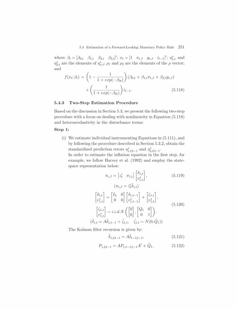
5.4 Estimation of a Forward-Looking Monetary Policy Rule 251
where βt = [β0,t β1,t β2,t β3,t]′; xt = [1 πt,J gt,J it−1]′; η∗1,t and
η∗2,t are the elements of η∗
x,t; ρ1 and ρ2 are the elements of the ρ vector;and
f(xt;βt) =(
1 − 11 + exp(−β3t)
)(β0,t + β1,tπt,J + β2,tgt,J)
+(
11 + exp(−β3t)
)it−1. (5.118)
5.4.3 Two-Step Estimation Procedure
Based on the discussion in Section 5.3, we present the following two-stepprocedure with a focus on dealing with nonlinearity in Equation (5.118)and heteroscedasticity in the disturbance terms:
Step 1:
(i) We estimate individual instrumenting Equations in (5.111), andby following the procedure described in Section 5.3.2, obtain thestandardized prediction errors η∗
1,t|t−1 and η∗2,t|t−1.
In order to estimate the inflation equation in the first step, forexample, we follow Harvey et al. (1992) and employ the state-space representation below:
πt,J =[z′t σ1,t
][δ1,t
v∗1,t
], (5.119)
(πt,J = z′tδ1,t)[
δ1,t
v∗1,t
]=[IL 00 0
][δ1,t−1
v∗1,t−1
]+[ζ1,t
v∗1,t
],
[ζ1,t
v∗1,t
]∼ i.i.d.N
([00
],
[Q1 00 1
]).
(5.120)
(δ1,t = Aδ1,t−1 + ζ1,t, ζ1,t ∼ N(0, Q1))
The Kalman filter recursion is given by:
δ1,t|t−1 = Aδt−1|t−1, (5.121)
P1,t|t−1 = AP1,t−1|t−1A′ + Q1, (5.122)
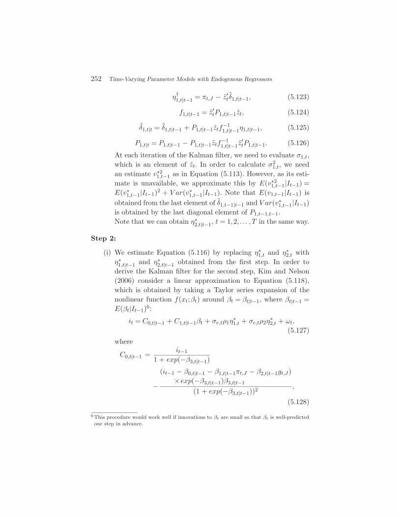
252 Time-Varying Parameter Models with Endogenous Regressors
η†1,t|t−1 = πt,J − z′
tδ1,t|t−1, (5.123)
f1,t|t−1 = z′tP1,t|t−1zt, (5.124)
δ1,t|t = δ1,t|t−1 + P1,t|t−1ztf−11,t|t−1η1,t|t−1, (5.125)
P1,t|t = P1,t|t−1 − P1,t|t−1ztf−11,t|t−1z
′tP1,t|t−1. (5.126)
At each iteration of the Kalman filter, we need to evaluate σ1,t,which is an element of zt. In order to calculate σ2
1,t, we needan estimate v∗2
1,t−1 as in Equation (5.113). However, as its esti-mate is unavailable, we approximate this by E(v∗2
1,t−1|It−1) =E(v∗
1,t−1|It−1)2 + V ar(v∗1,t−1|It−1). Note that E(v1,t−1|It−1) is
obtained from the last element of δ1,t−1|t−1 and V ar(v∗1,t−1|It−1)
is obtained by the last diagonal element of P1,t−1,t−1.Note that we can obtain η∗
2,t|t−1, t = 1,2, . . . ,T in the same way.
Step 2:
(i) We estimate Equation (5.116) by replacing η∗1,t and η∗
2,t withη∗1,t|t−1 and η∗
2,t|t−1 obtained from the first step. In order toderive the Kalman filter for the second step, Kim and Nelson(2006) consider a linear approximation to Equation (5.118),which is obtained by taking a Taylor series expansion of thenonlinear function f(xt;βt) around βt = βt|t−1, where βt|t−1 =E(βt|It−1)6:
it = C0,t|t−1 + C1,t|t−1βt + σe,tρ1η∗1,t + σe,tρ2η
∗2,t + ωt,
(5.127)
where
C0,t|t−1 =it−1
1 + exp(−β3,t|t−1)
−(it−1 − β0,t|t−1 − β1,t|t−1πt,J − β2,t|t−1gt,J)
×exp(−β3,t|t−1)β3,t|t−1
(1 + exp(−β3,t|t−1))2,
(5.128)
6 This procedure would work well if innovations to βt are small so that βt is well-predictedone step in advance.
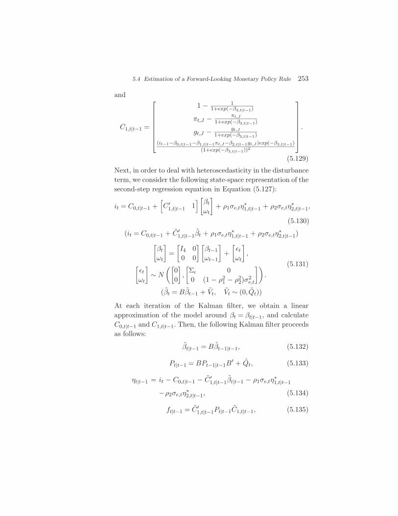
5.4 Estimation of a Forward-Looking Monetary Policy Rule 253
and
C1,t|t−1 =
1 − 11+exp(−β3,t|t−1)
πt,J − πt,J
1+exp(−β3,t|t−1)
gt,J − gt,J
1+exp(−β3,t|t−1)
(it−1−β0,t|t−1−β1,t|t−1πt,J−β2,t|t−1gt,J )exp(−β3,t|t−1)(1+exp(−β3,t|t−1))2
.
(5.129)
Next, in order to deal with heteroscedasticity in the disturbanceterm, we consider the following state-space representation of thesecond-step regression equation in Equation (5.127):
it = C0,t|t−1 +[C ′
1,t|t−1 1][βt
ωt
]+ ρ1σe,tη
∗1,t|t−1 + ρ2σe,tη
∗2,t|t−1,
(5.130)
(it = C0,t|t−1 + C ′1,t|t−1βt + ρ1σe,tη
∗1,t|t−1 + ρ2σe,tη
∗2,t|t−1)[
βt
ωt
]=[I4 00 0
][βt−1
ωt−1
]+[εtωt
],
[εtωt
]∼ N
([00
],
[Σε 00 (1 − ρ2
1 − ρ22)σ
2e,t
]).
(5.131)
(βt = Bβt−1 + Vt, Vt ∼ (0, Qt))
At each iteration of the Kalman filter, we obtain a linearapproximation of the model around βt = βt|t−1, and calculateC0,t|t−1 and C1,t|t−1. Then, the following Kalman filter proceedsas follows:
βt|t−1 = Bβt−1|t−1, (5.132)
Pt|t−1 = BPt−1|t−1B′ + Qt, (5.133)
ηt|t−1 = it − C0,t|t−1 − C ′1,t|t−1βt|t−1 − ρ1σe,tη
∗1,t|t−1
−ρ2σe,tη∗2,t|t−1, (5.134)
ft|t−1 = C ′1,t|t−1Pt|t−1C1,t|t−1, (5.135)
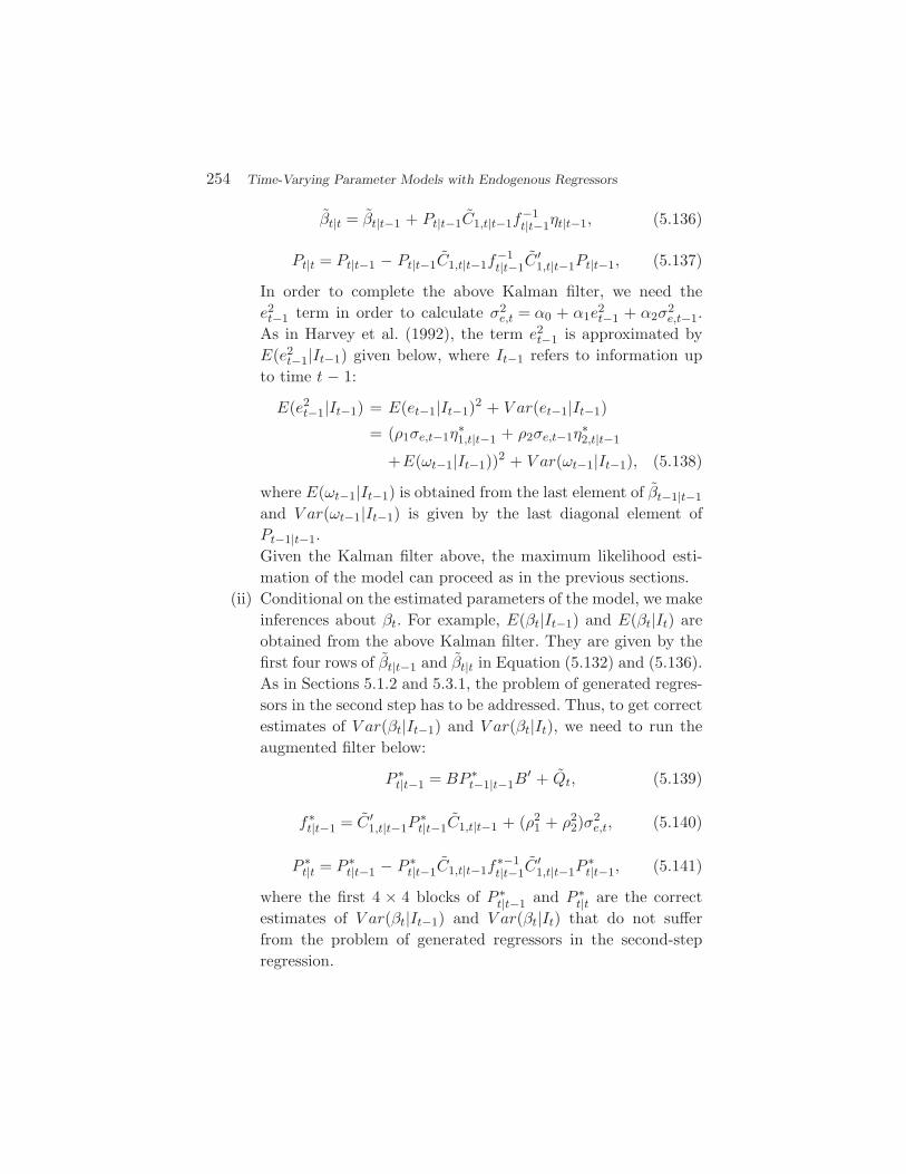
254 Time-Varying Parameter Models with Endogenous Regressors
βt|t = βt|t−1 + Pt|t−1C1,t|t−1f−1t|t−1ηt|t−1, (5.136)
Pt|t = Pt|t−1 − Pt|t−1C1,t|t−1f−1t|t−1C
′1,t|t−1Pt|t−1, (5.137)
In order to complete the above Kalman filter, we need thee2t−1 term in order to calculate σ2
e,t = α0 + α1e2t−1 + α2σ
2e,t−1.
As in Harvey et al. (1992), the term e2t−1 is approximated byE(e2t−1|It−1) given below, where It−1 refers to information upto time t − 1:
E(e2t−1|It−1) = E(et−1|It−1)2 + V ar(et−1|It−1)
= (ρ1σe,t−1η∗1,t|t−1 + ρ2σe,t−1η
∗2,t|t−1
+E(ωt−1|It−1))2 + V ar(ωt−1|It−1), (5.138)
where E(ωt−1|It−1) is obtained from the last element of βt−1|t−1and V ar(ωt−1|It−1) is given by the last diagonal element ofPt−1|t−1.Given the Kalman filter above, the maximum likelihood esti-mation of the model can proceed as in the previous sections.
(ii) Conditional on the estimated parameters of the model, we makeinferences about βt. For example, E(βt|It−1) and E(βt|It) areobtained from the above Kalman filter. They are given by thefirst four rows of βt|t−1 and βt|t in Equation (5.132) and (5.136).As in Sections 5.1.2 and 5.3.1, the problem of generated regres-sors in the second step has to be addressed. Thus, to get correctestimates of V ar(βt|It−1) and V ar(βt|It), we need to run theaugmented filter below:
P ∗t|t−1 = BP ∗
t−1|t−1B′ + Qt, (5.139)
f∗t|t−1 = C ′
1,t|t−1P∗t|t−1C1,t|t−1 + (ρ2
1 + ρ22)σ
2e,t, (5.140)
P ∗t|t = P ∗
t|t−1 − P ∗t|t−1C1,t|t−1f
∗−1t|t−1C
′1,t|t−1P
∗t|t−1, (5.141)
where the first 4 × 4 blocks of P ∗t|t−1 and P ∗
t|t are the correctestimates of V ar(βt|It−1) and V ar(βt|It) that do not sufferfrom the problem of generated regressors in the second-stepregression.
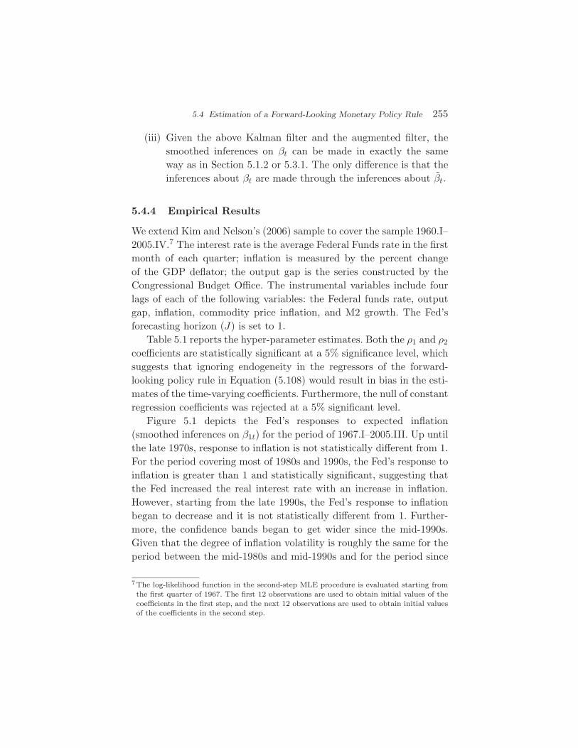
5.4 Estimation of a Forward-Looking Monetary Policy Rule 255
(iii) Given the above Kalman filter and the augmented filter, thesmoothed inferences on βt can be made in exactly the sameway as in Section 5.1.2 or 5.3.1. The only difference is that theinferences about βt are made through the inferences about βt.
5.4.4 Empirical Results
We extend Kim and Nelson’s (2006) sample to cover the sample 1960.I–2005.IV.7 The interest rate is the average Federal Funds rate in the firstmonth of each quarter; inflation is measured by the percent changeof the GDP deflator; the output gap is the series constructed by theCongressional Budget Office. The instrumental variables include fourlags of each of the following variables: the Federal funds rate, outputgap, inflation, commodity price inflation, and M2 growth. The Fed’sforecasting horizon (J) is set to 1.
Table 5.1 reports the hyper-parameter estimates. Both the ρ1 and ρ2
coefficients are statistically significant at a 5% significance level, whichsuggests that ignoring endogeneity in the regressors of the forward-looking policy rule in Equation (5.108) would result in bias in the esti-mates of the time-varying coefficients. Furthermore, the null of constantregression coefficients was rejected at a 5% significant level.
Figure 5.1 depicts the Fed’s responses to expected inflation(smoothed inferences on β1t) for the period of 1967.I–2005.III. Up untilthe late 1970s, response to inflation is not statistically different from 1.For the period covering most of 1980s and 1990s, the Fed’s response toinflation is greater than 1 and statistically significant, suggesting thatthe Fed increased the real interest rate with an increase in inflation.However, starting from the late 1990s, the Fed’s response to inflationbegan to decrease and it is not statistically different from 1. Further-more, the confidence bands began to get wider since the mid-1990s.Given that the degree of inflation volatility is roughly the same for theperiod between the mid-1980s and mid-1990s and for the period since
7 The log-likelihood function in the second-step MLE procedure is evaluated starting fromthe first quarter of 1967. The first 12 observations are used to obtain initial values of thecoefficients in the first step, and the next 12 observations are used to obtain initial valuesof the coefficients in the second step.
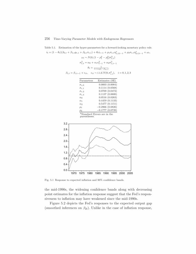
256 Time-Varying Parameter Models with Endogenous Regressors
Table 5.1. Estimation of the hyper-parameters for a forward-looking monetary policy rule.
it = (1 − θt)(β0,t + β1,tgt,1 + β2,tπt,1) + θtit−1 + ρ1σe,tη∗1,t|t−1 + ρ2σe,tη∗
2,t|t−1 + ωt,
ωt ∼ N(0,(1 − ρ21 − ρ2
2)σ2e,t)
σ2e,t = α0 + α1e2
t−1 + α2σ2e,t−1
θt = 11+exp(−β3,t)
βi,t = βi,t−1 + εit, εit ∼ i.i.d.N(0,σ2ε,i), i = 0,1,2,3
Parameters Estimates (SE)
σε,0 0.0003 (0.0084)σε,1 0.1114 (0.0568)σε,2 0.0709 (0.0472)σε,3 0.1137 (0.0600)α0 0.0516 (0.0263)α1 0.4459 (0.1133)α2 0.5477 (0.1151)ρ1 −0.2966 (0.0826)ρ2 −0.1777 (0.0739)
*Standard Errors are in theparentheses.
0.0
0.4
0.8
1.2
1.6
2.0
2.4
2.8
3.2
1970 1975 1980 1985 1990 1995 2000 2005
Fig. 5.1 Response to expected inflation and 90% confidence bands.
the mid-1990s, the widening confidence bands along with decreasingpoint estimates for the inflation response suggest that the Fed’s respon-siveness to inflation may have weakened since the mid-1990s.
Figure 5.2 depicts the Fed’s responses to the expected output gap(smoothed inferences on β2t). Unlike in the case of inflation response,
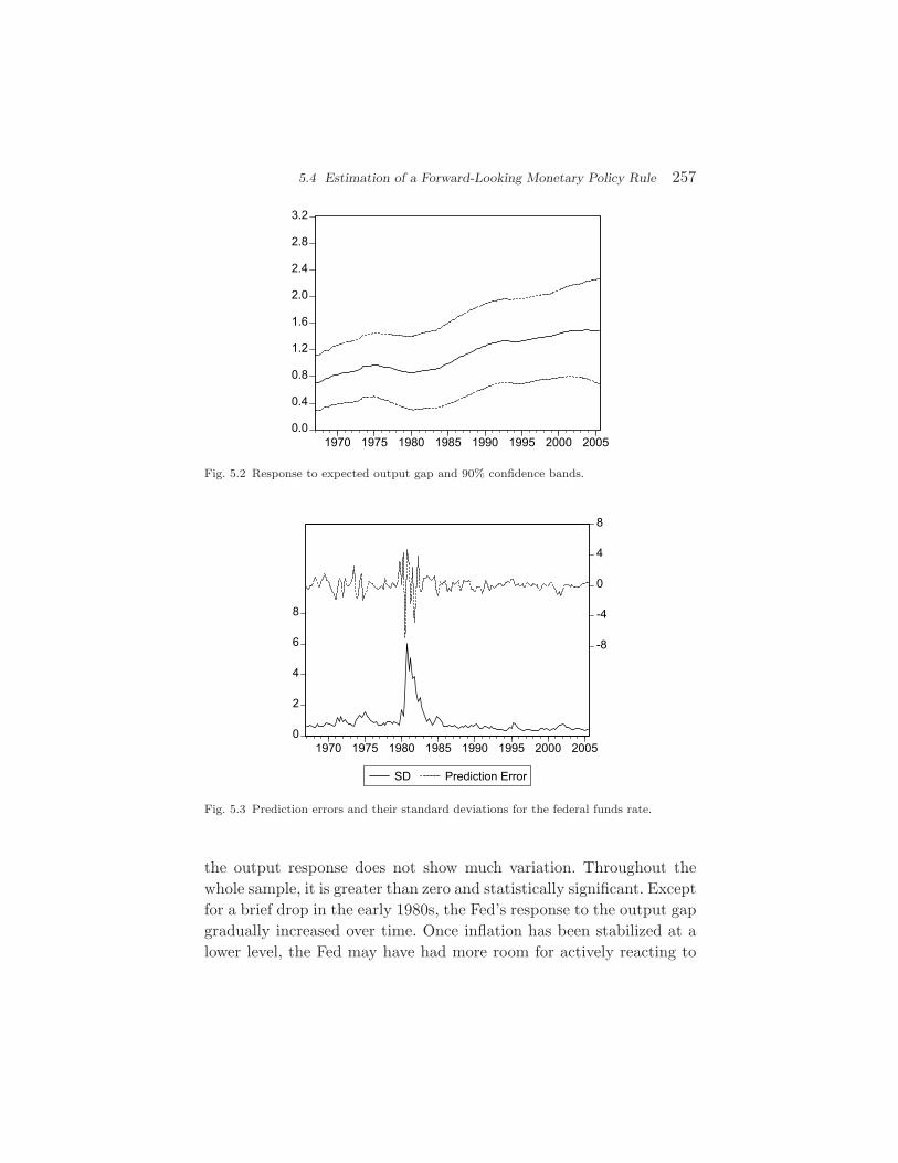
5.4 Estimation of a Forward-Looking Monetary Policy Rule 257
0.0
0.4
0.8
1.2
1.6
2.0
2.4
2.8
3.2
1970 1975 1980 1985 1990 1995 2000 2005
Fig. 5.2 Response to expected output gap and 90% confidence bands.
0
2
4
6
8
-8
-4
0
4
8
1970 1975 1980 1985 1990 1995 2000 2005
SD Prediction Error
Fig. 5.3 Prediction errors and their standard deviations for the federal funds rate.
the output response does not show much variation. Throughout thewhole sample, it is greater than zero and statistically significant. Exceptfor a brief drop in the early 1980s, the Fed’s response to the output gapgradually increased over time. Once inflation has been stabilized at alower level, the Fed may have had more room for actively reacting to
258 Time-Varying Parameter Models with Endogenous Regressors
real economic conditions such as the real GDP gap. Actually, the Fed’sresponse to real GDP gap since the 1990s is larger than ever before.
Finally, in Figure 5.3, the prediction errors and their conditionalstandard deviations for the federal funds rate are plotted. We canreconfirm the importance of incorporating heteroscedasticity in the dis-turbances of the monetary policy rule, as emphasized by Sims and Zha(2006).
6Concluding Remarks
In the empirical time series literature on instrumental variables (IV)or generalized methods of moments (GMM) estimation methods, thedynamic nature of the regression coefficients has usually been ignored.Similarly, in the empirical time series literature on dynamic regres-sion coefficients, problems arising from various types of endogeneityhave been usually ignored. With the advance of macroeconomic mod-els in which economic agents’ expectations of future macro variablesplay important roles (e.g., forward-looking new Keynesian models andforward-looking Taylor rule, etc.), and with the necessity to deal withunstable relationship among economic variables as shown by Stockand Watson (1998) and others, there has been high demand for timeseries models that can simultaneously deal with the issues of bothdynamic regression coefficients and endogeneity. The econometric mod-els reviewed in this monograph meet such a demand, and this articleprovides both the theoretical basis for estimation and the empiricalapplications of such models.
In this monograph, we have shown that the problem of endogeneityin Markov-switching models or time-varying parameter models can be
259

260 Concluding Remarks
easily solved by adopting a slightly modified version of the conventionalHamilton filter or the conventional Kalman filter. Easy methodsfor addressing the problem of generated regressors in the two-stepestimation procedures have also been presented.
References
Adam, K. and M. Padula (2003), ‘Inflation dynamics and subjectiveexpectations in the United States’. ECB Working Paper No. 222.
Belsley, D. (1973), ‘On the determination of systematic parameter vari-ation in the linear regression model’. Annals of Economic and SocialMeasurement 2, 487–494.
Boivin, J. (2006), ‘Has U.S. monetary policy changed? Evidence fromdrifting coefficients and real-time data’. Journal of Money, Creditand Banking 38(5), 1149–1174.
Campbell, J. Y. and L. Hentschel (1992), ‘No news is good news: Anasymmetric model of changing volatility in stock returns’. Journal ofFinancial Economics 31, 281–318.
Campbell, J. Y. and N. G. Mankiw (1989), ‘Consumption, income, andinterest rates: Reinterpreting the time series evidence’. In: O. J. Blan-chard and S. Fischer (eds.): National Bureau of Economic ResearchMacroeconomics Annual 1989. Cambridge, MA: MIT Press, pp. 185–216.
Campbell, J. Y. and N. G. Mankiw (1991), ‘The response of consump-tion to income: A cross-country investigation’. European EconomicReview 35, 723–67.
261
262 References
Carroll, C. (2003), ‘Macroeconomic expectations of households andprofessional forecasters’. Quarterly Journal of Economics 118(1),269–298.
Chib, S. (1998), ‘Estimation and comparison of multiple change-pointmodels’. Journal of Econometrics 86, 221–241.
Chow, G. C. (1984), ‘Random and changing coefficient models’. In:Z. Griliches and M. D. Intriligator (eds.): Handbook of Econometrics.North Holland: Amsterdam, Chapter 21.
Christiano, L. J., M. Eichenbaum, and C. L. Evans (2005), ‘Nominalrigidities and the dynamic effects of a shock to monetary policy’.Journal of Political Economy 113(1), 1–45.
Clarida, R., J. Gali, and M. Gertler (2000), ‘Monetary policy rulesand macroeconomic stability: Evidence and some theory’. QuarterlyJournal of Economics pp. 147–180.
Cogley, T. and T. J. Sargent (2002), ‘Evolving post-world war II U.S.inflation dynamics’. In: NBER Macroeconomics Annual 16. Cam-bridge, MA: MIT Press, pp. 331–373.
Cogley, T. and T. J. Sargent (2005), ‘Drifts and volatilities: Monetarypolicies and outcomes in the post world war II U.S.’. Review of Eco-nomic Dynamics 8, 262–302.
Cogley, T. and A. M. Sbordone (2008), ‘Trend inflation, indexation, andinflation persistence in the New Keynesian Phillips curve’. AmericanEconomic Review 98(5), 2101–2126.
Cooley, T. F. and E. C. Prescott (1973), ‘Varying parameter regression:A theory and some applications’. Annals of Economic and SocialMeasurement 2, 463–473.
Cooley, T. F. and E. C. Prescott (1976), ‘Tests of an adaptive regressionmodel’. Estimation in the Presence of Stochastic Parameter Varia-tion, Econometrica 44, 167–184.
Diebold, F. X. (1998), ‘The past, present, and future of macroeco-nomics’. Journal of Economic Perspectives 12, 175–19.
Diebold, F. X., J.-H. Lee, and G. C. Weinbach (1994), ‘Regimeswitching with time-varying transition probabilities’. In: C. Harg-reaves (ed.): Nonstationary Time Series Analysis and Cointegration.Oxford: Oxford University Press.
References 263
Engle, R. F. and M. W. Watson (1987), ‘The Kalman filter model:Applications to forecasting and rational expectations’. In: T. Bewley(ed.): Advances in Econometrics: Fifth World Congress of Econo-metric Society. Cambridge, U.K.: Cambridge University Press.
Erceg, C. J. and A. T. Levin (2003), ‘Imperfect credibility and inflationpersistence’. Journal of Monetary Economics 50, 915–944.
Filardo, A. J. (1994), ‘Business-cycle phases and their transitionaldynamics’. Journal of Business and Economic Statistics 12, 299–308.
Fuhrer, J. C. (1997), ‘Inflation/output variance trade-offs and opti-mal monetary policy’. Journal of Money, Credit, and Banking 29,214–234.
Fuhrer, J. C. and G. R. Moore (1995), ‘Inflation persistence’. QuarterlyJournal of Economics 110, 127–159.
Gali, J. and M. Gertler (1999), ‘Inflation dynamics: A structural econo-metric analysis’. Journal of Monetary Economics 44(2), 195–222.
Gali, J., M. Gertler, and J. D. Lopez-Salido (2001), ‘European inflationdynamics’. European Economic Review 44(7), 1237–1270.
Goldfeld, S. M. and R. E. Quandt (1973), ‘A Markov model for switch-ing regressions’. Journal of Econometrics 1, 3–16.
Hamilton, J. D. (1989), ‘A new approach to the economic analysisof nonstationary time series and the business cycle’. Econometrica57(2), 357–384.
Harvey, A. C. (1981), Time Series Models. Oxford: Philip Allan andHumanities Press.
Harvey, A. C. (1991), Forecasting, Structural Time Series Models, andthe Kalman Filter. Cambridge, U.K.: Cambridge University Press.
Harvey, A. C., E. Ruiz, and E. Sentana (1992), ‘Unobserved componenttime series models with ARCH disturbances’. Journal of Economet-rics 52, 129–157.
Heckman, J. (1979), ‘Sample selection bias as a specification error’.Econometrica 47(1), 153–162.
Kalman, R. E. (1960), ‘A new approach to linear filtering and predictionproblems’. Transactions of the ASME Journal of Basic EngineeringD82, 35–45.
Kim, C.-J. (1994), ‘Dynamic linear models with Markov-switching’.Journal of Econometrics 60, 1–22.
264 References
Kim, C.-J. (2004), ‘Markov-switching models with endogenous explana-tory variables’. Journal of Econometrics 122, 127–136.
Kim, C.-J. (2006), ‘Time-varying parameter models with endogenousregressors’. Economic Letters 91, 21–26.
Kim, C.-J. (2009), ‘Markov-switching models with endogenous explana-tory variables II: A two-step MLE procedure’. Journal of Economet-rics 148, 46–55.
Kim, C.-J. and S. Chaudhuri (2009), ‘Markov-switching models withendogenous explanatory variables: Generalization’. Working Paper,University of Washington and University of North Carolina.
Kim, C.-J. and Y. Kim (2008), ‘Is the backward-looking componentimportant in a New Keynesian Phillips curve?’. Studies in NonlinearDynamics and Econometrics 12(3), Article 5.
Kim, C.-J., J. C. Morley, and C. R. Nelson (2004), ‘Is therea positive relationship between stock market volatility and theequity premium?’. Journal of Money, Credit and Banking 36,339–360.
Kim, C.-J. and C. R. Nelson (1999), State-Space Models with Regime-Switching: Classical and Gibbs-Sampling Approaches with Applica-tions. MIT Press.
Kim, C.-J. and C. R. Nelson (2006), ‘Estimation of a forward-lookingmonetary policy rule: A time-varying parameter model using ex-postdata’. Journal of Monetary Economics 53, 1949–1966.
Kim, C.-J., J. Piger, and R. Startz (2008), ‘Estimation of Markovregime-switching regression models with endogenous switching’.Journal of Econometrics 143(2), 263–273.
Kim, Y. and C.-J. Kim (2009), ‘Dealing with endogeneity in a time-varying-parameter model: Joint estimation and two-step estima-tion procedures’. Working Paper, University of Washington andUniversity of Manitoba.
Kozicki, S. and P. A. Tinsley (2001), ‘Term structure views of monetarypolicy under alternative models of agent expectations’. Journal ofEconomic Dynamics and Control 23, 149–184.
Kozicki, S. and P. A. Tinsley (2002), ‘Alternative sources of the lagdynamics of inflation’. Federal Reserve Bank of Kansas City, RWP02-12.
References 265
Lucas, R. E. (1976), ‘Econometric policy evaluation: A critique’.Carnegie-Rochester Conference Series on Public Policy 1, 19–46.
Maddala, G. and F. Nelson (1974), ‘Maximum likelihood methods formodels of markets in disequilibrium’. Econometrica 42(6), 1013–1030.
Maddala, G. S. (1983), Limited-Dependent and Qualitative Variables inEconometrics. Econometric Society Monographs No. 3, CambridgeUniversity Press.
Maddala, G. S. and F. Nelson (1975), ‘Switching regression models withexogenous and endogenous switching’. Proceedings of the AmericanStatistical Association pp. 423–426.
Monokroussos, G. (2009), ‘Dynamic limited dependent variable mod-eling and U.S. Monetary policy’. Forthcoming, in Journal of Money,Credit, and Banking.
Orphanides, A. (2004), ‘Monetary policy rules, macroeconomic stabilityand inflation: A view from the trenches’. Journal of Money, Creditand Banking 35(6).
Pagan, A. (1984), ‘Econometric issues in the analysis of regressionswith generated regressors’. International Economic Review 25(1),221–247.
Perron, P. and J. Qu (2007), ‘Estimating and testing multiple struc-tural changes in multivariate regressions’. Econometrica 75(2007),459–502.
Primiceri, G. E. (2005), ‘Time varying structural vector autoregressionsand monetary policy’. Review of Economic Studies 72, 821–852.
Quandt, R. E. (1958), ‘The estimation of the parameters of a lin-ear regression system obeying two separate regimes’. Journal of theAmerican Statistical Association 53, 873–880.
Roberts, J. M. (1995), ‘New Keynesian economics and the Phillipscurve’. Journal of Money, Credit and Banking 27(4), 975–984.
Roberts, J. M. (1997), ‘Is inflation sticky?’. Journal of MonetaryEconomics 39, 176–196.
Roberts, J. M. (1998), ‘Inflation expectations and the transmissionof monetary policy’. Federal Reserve Board FEDS working paper1998-43.
266 References
Rosenberg, B. (1973), ‘The analysis of a cross-section of time series bystochastically convergent parameter regression’. Annals of Economicand Social Measurement 2, 399–428.
Sarris, A. H. (1973), ‘A bayesian approach to estimation of time-varyingregression coefficients’. Annals of Economic and Social Measure-ment 2, pp. 501–524.
Sbordone, A. (2001), ‘Price and unit labor costs: A new test of pricestickiness’. Journal of Monetary Economics 49, 265–292.
Sbordone, A. (2002), ‘An optimizing model of U.S. wage and pricedynamics’. Proceedings, Federal Reserve Bank of San Francisco, Mar.
Sims, C. A., D. F. Waggoner, and T. Zha (2008), ‘Methods for infer-ence in large multiple-equation Markov-switching models’. Journalof Econometrics 146, 255–274.
Sims, C. A. and T. Zha (2006), ‘Were there regime switches in USMonetary policy?’. American Economic Review 96(1), 54–81.
Stock, J. H. and M. W. Watson (1998), ‘Evidence on structural insta-bility in macroeconomic time series relations’. Journal of Businessand Economic Statistics 14, 11–30.
Turner, C. M., R. Startz, and C. R. Nelson (1989), ‘A Markov modelof heteroscedasticity, risk, and learning in the stock market’. Journalof Financial Economics 25, 3–22.