arX

iv:1

405.

1964

v1 [

cs.G

T]

8 M

ay 2

014

A Distributed Demand-Side Management Framework for the

Smart Grid

Antimo Barbatoa, Antonio Caponea,∗, Lin Chenb, Fabio Martignonb,c, Stefano Parisd

aDEIB, Politecnico di Milano, via Ponzio 34/5, 20133 Milano, Italy.bLRI, Universit Paris-Sud, Bat. 650, rue Noetzlin, 91405 Orsay, France.

cIUF, Institut Universitaire de FrancedParis Descartes University, 45 rue des Saints Peres, 75270 Paris, France.

Abstract

This paper proposes a fully distributed Demand-Side Management system for Smart

Grid infrastructures, especially tailored to reduce the peak demand of residential users.

In particular, we use a dynamic pricing strategy, where energy tariffs are function of

the overall power demand of customers. We consider two practical cases: (1) a fully

distributed approach, where each appliance decides autonomously its own scheduling,

and (2) a hybrid approach, where each user must schedule all his appliances. We analyze

numerically these two approaches, showing that they are characterized practically by the

same performance level in all the considered grid scenarios.

We model the proposed system using a non-cooperative game theoretical approach,

and demonstrate that our game is a generalized ordinal potential one under general

conditions. Furthermore, we propose a simple yet effective best response strategy that

is proved to converge in a few steps to a pure Nash Equilibrium, thus demonstrating the

robustness of the power scheduling plan obtained without any central coordination of

the operator or the customers. Numerical results, obtained using real load profiles and

appliance models, show that the system-wide peak absorption achieved in a completely

distributed fashion can be reduced up to 55%, thus decreasing the capital expenditure

(CAPEX) necessary to meet the growing energy demand.

Keywords: Demand Management System, Power Scheduling, Load-Shifting, Game

Theory, Potential Games.

∗Corresponding author, Tel: (+39) 02.2399.3449, Fax: (+39) 02.2399.3413Email addresses: antimo.barbato@polimi.it (Antimo Barbato), antonio.capone@polimi.it

(Antonio Capone), lin.chen@lri.fr (Lin Chen), fabio.martignon@lri.fr (Fabio Martignon),stefano.paris@parisdescartes.fr (Stefano Paris)

Preprint submitted to Elsevier Computer Communications May 9, 2014

1. Introduction

The electricity generation, distribution and consumption are in the throes of change

due to significant regulatory, societal and environmental developments, as well as tech-

nological progress. Recent years have witnessed the redefinition of the power grid in

order to tackle the new challenges that have emerged in electric systems. One of the

most relevant challenges associated with the current power grid is represented by the

peaks in the power demand due to the high correlation among energy demands of cus-

tomers. Since electricity grids have little capacity to store energy, power demand and

supply must balance at all times; as a consequence, energy plants capacity has to be sized

to match the total demand peaks, driving a major increase of the infrastructure cost,

which remains underutilized during off-peak hours. This waste of resources has become

an even more critical issue in the last few years due to the increase of the worldwide

energy consumption [1] and the increasing share of renewable energy sources [2]. High

energy peaks are mostly due to residential users, who cover a relevant portion of the

worldwide energy demands [3], but are inelastic with respect to the grid requirements as

they usually run their home appliances only depending on their own requirements. For

this reason, residential users can play a key role in addressing the peak demand problem.

Time-Of-Use (TOU) tariffs represent a clear attempt to incite users to shift their energy

loads out of the peak hours [4].

The most promising solution to tackle the peak demand challenge is represented by

the Smart Grid, in which an intelligent infrastructure based on Information and Com-

munication Technology (ICT) tools is deployed alongside with the distribution network,

which can deal with all the decision variables while minimizing the effort required to

end-users. All data provided by the grid, such as the consumption of buildings [5] [6],

electricity costs and distributed Renewable Energy Sources (RESs) data, can be used

to optimize its efficiency through Demand-Side Management (DSM) methods, which

represent a proactive approach to manage the household electric devices by integrating

customers’ needs and requirements with the retailers’ goals [7]. The main objective of

these methods is to modify consumers’ energy demand in a proper way by deciding when

and how to execute home appliances so as to improve the overall system efficiency while

guaranteeing low costs and high comfort to users.

2

In this paper we propose a novel, fully distributed DSM system aimed at reducing

the peak demand of a group of residential users (e.g., a smart city neighborhood). In

particular, we consider a dynamic pricing strategy, where energy tariffs are function of

the overall power demand of customers.

We model our system using a game theoretical approach, considering two practical

cases where (1) each appliance decides autonomously its scheduling in a fully distributed

fashion (Single-Appliance DSM), and (2) each user must schedule all his home appliances

(Multiple-Appliance DSM). The proposed approach automatically ensures the reduction

of the electricity demand at peak hours due to dynamic pricing.

We compare numerically these two cases, showing that the first is characterized only

by a negligible performance degradation in all the considered grid scenarios. Neverthe-

less, while both mechanisms achieve almost the same performance level, the Multiple-

Appliance DSM system requires a more complex architecture with a central server for

each house that collects all appliances information and plays on behalf of the house-

holder. Such an approach would increase the installation and operating costs due to the

higher system complexity. On the contrary, in the Single-Appliance DSM system, one

can use the processing and communication capabilities of devices that can autonomously

optimize their usage, thus greatly simplifying the architecture design and system config-

uration. This solution is made possible by the diffusion of Smart Appliances that are

no longer merely passive devices, but active participants in the power grid infrastructure

[8].

We underline that, while recent literature has focused on the design of DSM systems

for controllable devices [9], namely devices whose power load profile within their operating

time can be modulated according to the DSM goals, our work designs a distributed DSM

to select the best (cheapest) schedule for shiftable appliances. Indeed, differently from air

conditioning or heating systems, appliances like the washing machine and the electric oven

have a fixed power profile optimized for specific goals. In such cases, a user can choose

the starting time for each shiftable appliance, whose power profile is fixed. Therefore,

our scheme is complementary to the approaches devised for controllable devices.

We demonstrate that our game is a generalized ordinal potential game [10] under some

simple and very general conditions (viz., the regularity of the pricing function). Such

3

feature guarantees some nice properties, such as the existence of at least one pure Nash

equilibrium (where no player has an incentive to deviate unilaterally from the scheduling

pattern he decided upon). Furthermore, we show that any sequence of asynchronous

improvement steps is finite and always converges to a pure Nash equilibrium.

In summary, our paper makes the following contributions:

• The proposition of a novel, fully distributed DSM method, able to reduce the

peak demand of a group of residential users, which we model and study using a

game theoretical framework. In our vision, the energy retailer fixes the energy

price dynamically, based on the total power demand of customers; then, appliances

autonomously decide their schedule, reaching an efficient Nash equilibrium point.

• Mathematical proofs that our proposed game is a generalized ordinal potential

game, under general conditions.

• The demonstration of the Finite Improvement Property, according to which any

sequence of asynchronous improvement steps (and, in particular, best response dy-

namics) converges to a pure Nash equilibrium.

• A thorough numerical evaluation that shows the effectiveness of the proposed ap-

proach in several scenarios, with real electric appliances scheduled by householders.

The paper is organized as follows. Section 2 discusses related work. Section 3 de-

scribes the main characteristics of the distributed system we propose to manage the

energy consumption of residential users. Section 4 presents our proposed game theoret-

ical formulation for the Single and Multiple-Appliance DSM, as well as the structural

properties of our game. Numerical results are presented and analyzed in Section 5.

Finally, Section 6 concludes the paper.

2. Related Work

Demand-Side Management (DSM) mechanisms have recently gained attention by the

scientific community due to their advantages in terms of wise use of energy and cost

reduction [11]. In DSM systems proposed in the literature, a mechanism is defined that,

based on energy tariffs and data forecasts for future periods (e.g., photovoltaic power4

generation, devices future usage), is able to automatically and optimally schedule the

home devices activities for future periods and to define the whole energy plan of users

(i.e., when to buy and sell energy to the grid). The main goal of these solutions is to

minimize the electricity costs while guaranteeing the users’ comfort; this can be achieved

through the execution of methods based on optimization models [12], [13] or heuristics,

such as Genetic Algorithms [14] and customized Evolutionary Algorithms [15], which are

used to solve more complex formulations of the demand management problem. Since

RESs diffusion is rapidly increasing, several works include renewable plants into DSM

frameworks. In these cases, devices are scheduled also based on the availability of an

intermittent electricity source (e.g., PV plants) and users’ profits from selling renew-

able electricity to the energy market are taken into account [16]. The uncertainty of

RESs generation forecasts is tackled through stochastic approaches, such as stochastic

dynamic programming which is a very suitable tool to address the decision-making pro-

cess of energy management systems in presence of uncertainty, such as the one related to

the electricity produced from weather-dependent generation sources [17]. The efficiency

of demand management solutions can be notably improved by including storage systems

that can increase the DSM flexibility in optimizing the usage of electric resources. Specif-

ically, batteries can be used to harvest the renewable generation in excess for later use

or to charge the ESS when the electricity price is low, with the goal of minimizing the

users’ electricity bill [18].

Solutions [12]–[18] are based on a single-user approach in which the energy plans of res-

idential customers are individually and locally optimized. However, in order to achieve

relevant results from a system-wide perspective, the energy management problem could

be applied to groups of users (e.g., a neighborhood or micro-grids), instead of single

users. For this reason, some preliminary solutions have been proposed in the literature

to manage energy resources of groups of customers. In [19], for example, the energy

bill minimization problem is applied to a group of cooperative residential users equipped

with PV panels and storage devices (i.e., electric vehicle batteries). A global scale op-

timization method is also proposed in [20], in which an algorithm is defined to control

domestic electricity and heat demand, as well as the generation and storage of heat and

electricity of a group of houses. These multi-user solutions require some sort of cen-

5

tralized coordination system run by the operator in order to collect all energy requests

and find the optimal solution. To this end, a large flow of data must be transmitted

through the Smart Grid network, thus introducing scalability constraints and requiring

the definition of high-performance communication protocols. Furthermore, the coordina-

tion system should also verify that all customers comply with the optimal task schedule,

since the operator has no guarantee that any user can gain by deviating unilaterally from

the optimal solution. Therefore, the collection of users’ metering data and the enforcing

of the optimal appliance schedule can introduce novel threats to customers’ security and

privacy. For these reasons, some distributed DSM methods have been proposed in which

decisions are taken locally, directly by the end consumer. In this case, Game Theory

represents the ideal framework to design DSM solutions. Specifically, in [9] a distributed

DSM system among users is proposed, where the users’ energy consumption scheduling

problem is formulated as a game: the players are the users, and their strategies are the

daily schedules of their household appliances and loads. The goal of the game is to either

reduce the peak demand or the energy bill of users. A game theoretical approach is also

used in [21], in which a distributed load management is defined to control the power

demand of users through dynamic pricing strategies. However, in these works, a very

simplified mathematical description is used to model houses, which does not correspond

to real use cases.

In this paper we propose a DSM method, based on a game theoretical approach,

which overcomes the most important limitations of the works proposed in the literature

and described above. Our DSM is a fully distributed system, in which no centralized

coordination is required, and only a limited and aggregated amount of data needs to

be transmitted between the operator and the householders through the Smart Grid.

For these reasons, scalability, communication, privacy and security issues are greatly

mitigated. Moreover, a realistic model of household contexts is illustrated; specifically,

a mathematical description of home devices is provided. Devices are defined as non-

preemptable activities characterized by specific load consumption profiles, determined

based on real data, and are scheduled according to users’ preferences defined based on

real use-case scenarios. Finally, to the best of our knowledge, the single-appliance demand

management game proposed in this paper, in which electric devices can autonomously

6

and locally optimize their usage, has never been studied in the literature.

3. System Model

The power scheduling system here proposed is designed to manage the electric appli-

ances of a group of residential users consisting of a set H of houses (e.g., a smart city

neighborhood). This system is used to schedule the energy plan of the whole group of

users over a 24-hour time horizon based on a fully distributed approach, with the final

goal of improving the efficiency of the whole power grid by reducing the peak demand of

electricity, while still complying with users’ needs and preferences. More specifically, in

our model we represent the daily time as a set T of time slots. Each householder 1 h ∈ H

has a set of non-preemptive electric appliances, A, that must be executed during the

day. In particular, the load profile of each appliance is modeled as an ordered sequence

of phases, F , in which a certain amount of power is consumed. We assume that the

power consumption lahf of a device a ∈ A belonging to user h ∈ H in each phase f ∈ F

is an average of the real consumption of the device within the time slot duration (see

Figure 1, where 15-minute phases are used for a washing machine [22]).

Each device a of user h needs to run for dah consecutive slots within a total of Rah

slots delimited by a minimum starting time slot, STah, and a maximum ending time slot,

ETah (verifying the constraint STah ≤ ETah−dah+1). These two parameters, STah and

ETah, represent the users’ preferences in starting each home device; they can be directly

provided by users or automatically obtained through learning algorithms such as the one

presented in [23].

In our model, we consider two different kinds of devices:

• Shiftable appliances (e.g., washing machine, dishwasher): they are manageable

devices that must be scheduled and executed during the day. In particular, for

each shiftable device a ∈ A of the householder h ∈ H, the minimum starting time

and the maximum ending time verify the constraint STah < ETah−dah+1. Hence,

their scheduling is an optimization variable in our model.

1In this paper, we use the terms householder and user interchangeably.

7

1 2 3 4 5 6 70

0,20,40,60,81,01,21,41,61,82,0

Phase

Pow

er (

kW)

Figure 1: Example of a load profile lahf of a washing machine.

• Fixed appliances (e.g., light, TV) are non-manageable devices, for which the start-

ing/ending times are fixed and cannot be optimized. More specifically, for each

fixed device a ∈ A of the householder h ∈ H, the minimum starting time and the

maximum ending time verify the constraint STah = ETah − dah + 1.

Devices scheduling is represented by the binary variable xaht, which is defined for

each appliance a ∈ A of each householder h ∈ H, and for each time slot t ∈ T . It

is equal to 1 if appliance a starts in time slot t, 0 otherwise. In order to use home

appliances, householders can buy energy from the electricity retailer. In particular, the

power demand of user h at time t is denoted by yht. The power demand of each user

cannot exceed a supply limit defined by the retailer and denoted by πSL; this limit

represents the maximum power that can be used at any time.

In our model, we have decided to use a dynamic pricing approach to define the

electricity tariff since it represents a very promising method to improve the efficiency

of the whole power grid [24]. Since the higher the demand of electricity, the larger

the capacity of grid generation and distribution to install, we suppose that the price of

electricity at time t, ct(·), is an increasing function of the total demand, yt, of the group

of users H at time t. Specifically, if the power demand is lower than a threshold πTT ,

ct(·) is a strictly increasing function of yt, otherwise it becomes a constant function of

value ct(πTT ).

The objective of the power scheduling system is to reduce the daily bill of each user,

by optimally scheduling house appliance activities and managing the power absorption

8

from the grid. Intuitively, based on the definition of the electricity price, by reducing the

users’ bills, the model is able to decrease the corresponding peak demand.

Table 1 summarizes the notation used in the paper.

Table 1: Basic notation used in the paper.

xaht Binary variable that indicates if appliance a

of householder h starts its execution at time t

yht Power demand of user h at time t

yt Total power demand at time t

ct(·) Pricing function

πTT Tariff Threshold of the pricing function

πSL Power Supply Limit

lahf Consumption of device a of user h in phase f

dah Operating time slots for device a of user h

STah/ETah Starting/Ending time for device a of user h

4. Distributed Power Scheduling as a Non-cooperative Game

In this section, we model the distributed power scheduling problem, which consti-

tutes the core of our proposed DSM system, using a non-cooperative game theoretical

approach (formally described in Definition 1), which naturally captures the interactions

in such a distributed decision making process. Our design rationale (Subsection 4.1) is

the following: each appliance a ∈ A is an autonomous decision maker (or player) that

must select the starting time of its execution (i.e., the xaht value); this permits to mini-

mize the coordination required by a central server that would operate at each house to

aggregate all appliances load and scheduling constraints. Consequently, each appliance a

decides autonomously when to buy energy from the grid (i.e., yht) in order to minimize

its contribution to the overall bill charged to house h ∈ H, according to his user’s2 needs.

Then, after having solved the single-appliance game and studied its structural prop-

erties (Subsection 4.2), in Subsection 4.3 we consider a natural (and more complex) ex-

2In this paper users are house owners, therefore we use interchangeably the terms house and user.

9

tension where a player represents an entire household which jointly decides the schedule

of all his appliances.

4.1. Single-Appliance Game Formulation

We first start describing the scenario where each appliance a ∈ A of house h ∈ H

is modeled as an autonomous player in the power scheduling game G, which is defined

as a triple {N , I,P}: N = A × H is the player set, I , {In}n∈N is the strategy set

with In , {xnt}n∈N being the strategy of player n, P , {Pn}n∈N is the cost function

of player n with Pn being the total price paid by n for its electricity consumption (the

total price due to appliance a ∈ A of house h ∈ H). Each appliance (player) n chooses

its strategy In to minimize its cost Pn.

The feasible power scheduling alternatives that form the strategy space In of each

player n = (a, h) (i.e., each appliance a of householder h) must satisfy both the consumer

needs and energy supply limits. Specifically, the strategy space In must satisfy the

following set of constraints:

In =

{

−→x n =[

xn1...xnt...xn|T |

]

∈ {0, 1}|T | :

ETn−dn+1∑

t=STn

xnt = 1 (1)

ynt =∑

f∈F:f≤t

lnfxn(t−f+1) ∀t ∈ T (2)

yht =∑

a∈A

∑

f∈F:f≤t

lahfxah(t−f+1) ∀t ∈ T (3)

yht ≤ πSL ∀t ∈ T

}

. (4)

Constraints (1) guarantee that appliance n starts in exactly one time slot and it is

carried out in the interval (STn, ETn). Constraints (2) determine the daily consumption

profile of the appliances in each time slot, which depends on their scheduling. More

specifically, the power required by each appliance in each time slot t, ynt, is equal to the

load profile lnf of the phase carried out at time t. Note that a phase f is running in

t, only if the appliance started at time t − f + 1, thus if xn(t−f+1) = 1. In a similar

fashion, equations (3) define the daily power demand of house h based on the appliances

scheduling. Finally, constraints (4) limit the overall power consumption of each house,

since in every time slot t ∈ T , the electricity bought from the grid cannot exceed the10

Supply Limit (SL) defined by the retailer and denoted by πSL. In such constraints, the

power required by each appliance in each time slot t, ynt, is equal to the load profile lnf

of the phase executed starting from the time slot where xnt = 1. Note that (2) is used

by the appliance a to compute and minimize its contribution to the overall price charged

to house h, whereas (3) is used by householder h to compute the bill.

Having defined the strategy space of each player, we can now define the single-

appliance power scheduling game.

Definition 1 (Power Scheduling Game). Mathematically, the power scheduling game is

formalized as follows:

G : minIn

Pn(In, I−n) =∑

t∈T

ynt · ct(yt), ∀n ∈ N . (5)

The solution of the power scheduling game is characterized by a Nash Equilibrium

(NE), a strategy profile I∗ = (I∗n, I

∗−n) from which no player has an incentive to deviate

unilaterally, i.e.,

Pn(I∗n, I

∗−n) ≥ Pn(In, I

∗−n), ∀n ∈ N , ∀In ∈ I.

To study the efficiency of the NE(s) of G, we define the social cost of all players

as the total price, P , paid by all customers to the electricity retailer, as a function of

I = {In}n∈N , where the strategy of player n is In = {xnt}n∈N :

P (I) =∑

h∈H

∑

t∈T

yht · ct(yt), (6)

where yht is a function of xnt, n = (a, h) ∈ A×H and ct is a function of yt that represents the

total power demand of all players at time t.

By analyzing the utility functions of G, we can see that the pricing function ct(yt)

plays an important role on the resulting system equilibrium point(s). Specifically, our

objective is to devise smart pricing policies to drive the system equilibrium to the op-

timum in terms of social cost. In this regard, we focus on a class of pricing functions,

termed as regular pricing functions, defined as follows.

Definition 2 (Regular Pricing Function). The pricing function {ct(yt)}0≤t≤T is a regular

pricing function if the following properties hold:11

• ct(yt) is continuous, non-decreasing for 0 ≤ t ≤ T and its derivative c′t(yt) is

continuous in yt;

• Given any two time intervals [t0u, t1u], [t0v, t

1v] and power demand in these inter-

vals {yu}t0u<u<t1

u, {yv}t0

v<v<t1

v, if

∑t1u

u=t0u

c′u(yu) >∑t1

v

v=t0v

c′v(yv), then it holds that∑t1

u

u=t0u

[yucu(yu)]′ >

∑t1v

v=t0v

[yvcv(yv)]′.

Remark: Regular pricing functions characterize a family of utility functions widely

applied in practical applications. A typical example of regular pricing function is the

power function ct = αyβt where α > 0 and β ≥ 1. The design motivation hinging

behind such pricing functions is to encourage users to balance their electricity demand

and consequently decrease the peak demand.

In the following analysis, we show that under the condition that the pricing policy

can be expressed by a regular function, the power scheduling game G admits a number

of desirable properties, particularly from the perspective of social cost.

4.2. Solving the Power Scheduling Game

In this subsection, we solve the power scheduling game G and study the structural

properties of the game. We are specifically interested in large systems where the impact

of an individual user on the system dynamics is limited. Theorem 1 shows that G is a

generalized ordinal potential game, whose definition is reported hereafter for complete-

ness.

Definition 3 (Generalized Ordinal Potential Game). Given a finite strategic game

Γ , {N , {Sn}n∈N , {un}n∈N }, Γ is a generalized ordinal potential game if there exists

a function (called potential function) Φ : S → R such that for every player n ∈ N and

every s−n ∈ S−n and sn, s′n ∈ Sn, it holds that

un(sn, s−n) > un(s′n, s−n) =⇒ Φ(sn, s−n) > Φ(s′n, s−n).

Theorem 1. Under the condition that {ct(yt)}0≤t≤T is a regular pricing function, the

power scheduling game G is a generalized ordinal potential game with the corresponding

potential function being P (I)

12

Proof. To prove the theorem, it suffices to show that for any two strategies In and I ′n

and for any player n ∈ N , it holds that

Pn(In, I−n) > Pn(I′n, I−n) =⇒ P (In, I−n) > P (I ′

n, I−n).

In this regard, assume that Pn(In, I−n) > Pn(I ′n, I−n). Assume that n (i.e., appliance

a ∈ A of house h ∈ H) starts its activity in time interval t0u < u < t1u (t0v < v < t1v,

respectively) in strategy In (I ′n). Let yt denote the total power demand at time t under

strategy profile (In, I−n). Between the strategy profiles (In, I−n) and (I ′n, I−n), the

difference is that n migrates its power demand of pn from time interval [t0u, t1u] to [t0v, t

1v].

Since we are focused on large systems where the impact of an individual user on the

system dynamics is limited, i.e., pn ≪ yt, it holds that

Pn(In, I−n)− Pn(I′n, I−n) =

t1u

∑

u=t0u

pncu(yu) +

t1v

∑

v=t0v

pncv(yv)

−

t1u

∑

u=t0u

pncu(yu − pn) +

t1v

∑

v=t0v

pncv(yv + pn)

≃

≃ pn

t1u

∑

u=t0u

c′u(yu − pn)−

t1v

∑

v=t0v

c′v(yv)

> 0, (7)

following the assumption that Pn(In, I−n) > Pn(I ′n, I−n).

Recalling the definition of regular pricing functions, it then holds that

t1u

∑

u=t0u

[(yu − pn)cu(yu − pn)]′ >

t1v

∑

v=t0v

[yvcv(yv)]′. (8)

On the other hand, we study the social cost under the strategy profiles (In, I−n) and

(I ′n, I−n). Specifically, we can derive the difference between P (In, I−n) and P (I ′

n, I−n)

as follows:

P (In, I−n)− P (I′n, I−n) =

t1u

∑

u=t0u

[yucu(yu)] +

t1v

∑

v=t0v

[yvcv(yv)]

−

t1u

∑

u=t0u

[(yu − pn)cu(yu − pn)] +

t1v

∑

v=t0v

[(yv + pn)cv(yv + pn)]

=

t1u

∑

u=t0u

[yucu(yu)]−

t1u

∑

u=t0u

[(yu − pn)cu(yu − pn)]

−

t1v

∑

v=t0v

[(yv + pn)cv(yv + pn)]−

t1v

∑

v=t0v

[yvcv(yv)]

. (9)

13

With some algebraic operations, we have

t1u

∑

u=t0u

[yucu(yu)]−

t1u

∑

u=t0u

[(yu − pn)cu(yu − pn)] =

t1u

∑

u=t0u

{yu[cu(yu)− cu(yu − pn)] + pncu(yu − pn)} ≃

≃

t1u

∑

u=t0u

{yupnc′u(yu − pn) + pncu(yu − pn)} >

>

t1u

∑

u=t0u

[(yu − pn)cu(yu − pn)]′. (10)

Similarly, we have

t1v

∑

v=t0v

[(yv + pn)cv(yv + pn)]−

t1v

∑

v=t0v

[yvcv(yv)] <

t1v

∑

v=t0v

[yvcv(yv)]′. (11)

Hence, it follows from (10) and (11) that

P (In, I−n)− P (I′n, I−n) =

t1u

∑

u=t0u

[yucu(yu)]−

t1u

∑

u=t0u

[(yu − pn)cu(yu − pn)]

−

t1v

∑

v=t0v

[(yv + pn)cv(yv + pn)]−

t1v

∑

v=t0v

[yvcv(yv)]

>

>

t1u

∑

u=t0u

[(yu − pn)cu(yu − pn)]′ −

t1v

∑

v=t0v

[yvcv(yv)]′ > 0. (12)

The proof is thus completed.

Corollary 1 (Efficiency of the Equilibrium). Under the conditions of Theorem 1, the

equilibrium of G minimizes the total price paid to the operator, i.e., the total social cost.

Corollary 2 (Convergence to the Equilibrium). Under the conditions of Theorem 1, G

admits the Finite Improvement Property (FIP). Any sequence of asynchronous improve-

ment steps is finite and converges to a pure equilibrium. Particularly, the sequence of

best response updates converges to a pure equilibrium.

14

Potential games have nice properties, such as existence of at least one pure Nash

equilibrium, namely the strategy that minimizes P (I). Furthermore, in such games,

best response dynamics always converges to a Nash equilibrium.

Hereafter, we describe a simple implementation of best response dynamics, which

allows each player n, namely each appliance a of each householder h, to improve its cost

function in the proposed power scheduling game. Such algorithm is the best response

strategy for a player n minimizing objective function (5),∑

t∈T ynt · ct(yt), assuming

other appliances are not changing their strategies.

Specifically, each appliance, in an iterative fashion, defines its optimal power schedul-

ing strategy based on electricity tariffs (calculated according to other players’ strategies)

and broadcasts its energy plan (i.e., its daily power demand profile) to the group N . At

every iteration, energy prices are updated according to the last strategy profile and, as

a consequence, other appliances can decide to modify their consumption scheduling by

changing their strategy according to the new tariffs. The iterative process is repeated

until convergence is reached. Once convergence is reached, appliances power scheduling

and energy prices are fixed as well as the energy bill charged to each householder h,

which is simply the sum of all his appliances prices∑

t∈T yht · ct(yt).

The best response mechanism is executed by solving, in an iterative way, an optimiza-

tion model. Specifically, at every iteration and based on the energy demands of other

appliances, this model is used to optimally decide the power plan of the appliance in

charge of defining its energy demand at this step of the iterative process, with the goal

of minimizing the electricity bill. We will show in the Numerical Results section that our

proposed algorithm converges, in few iterations, to a Nash equilibrium.

Note that the best response dynamics here proposed is only used to identify and

study the efficiency of the Nash Equilibrium of the game. While the transmission of the

power profile to other users may raise security and privacy concerns, we observe that

each appliance needs only the aggregated power profile of other appliances for the real

implementation of the Single-Appliance DSM. Therefore, we can envisage a system in

which appliances communicate only with the operator that broadcasts the aggregated

information after collecting all appliance’s schedules. Furthermore, to completely remove

the communication of any sensitive information, any learning algorithm could be designed

15

to allow appliances to converge to the equilibrium.

4.3. Multiple-Appliance Game Formulation

The natural extension of the single-application power scheduling game considers as a

player the householder h who chooses the schedule of all his appliances according to his

preferences. The strategy space for player h is therefore composed of all variables xaht

corresponding to the activities of all his appliances.

Definition 4 (Multiple-Appliance Power Scheduling Game). Mathematically, the multiple-

appliances power scheduling game is formalized as follows:

G : minIh

Ph(Ih, I−h) =∑

t∈T

yht · ct(yt), ∀n ∈ N (13)

Ih =

{

Xh =

x1h1 x1ht · · · x1h|T |

x2h1 x2ht · · · x2h|T |

.

.

.

.

.

.

.

.

.

.

.

.

x|A|h1 x|A|ht · · · x|A|h|T |

∈ {0, 1}|A|×|T | :

ETah−dah+1∑

t=STah

xaht = 1 ∀a ∈ A (14)

yht =∑

a∈A

∑

f∈F:f≤t

lahfxah(t−f+1) ∀t ∈ T (15)

yht ≤ πSL ∀t ∈ T

}

. (16)

Similarly to (1), (3) and (4), constraints (14), (15) and (16) are used, respectively,

to guarantee that each appliance a starts in exactly one time slot within the interval

(STah, ETah), to define the daily power demand of house h and to upper-bound the

demand of each house according to the supply limit πSL.

We underline that scheduling optimally multiple appliances increases the complexity

of the Smart Grid architecture, since each house requires a central server that collects

the energy consumption information from all house appliances and the householder’s

preferences (i.e., starting/ending times). Conversely, in the single-appliance formulation

each appliance operates independently, and the householder can configure asynchronously

the different appliances preferences. Furthermore, as we will show in the next Section,

16

the higher complexity of the multiple-appliance scheduling game does not result in lower

costs for the householder or a lower power peak for the retailer’s grid.

5. Numerical Results

This section presents the numerical results we obtained evaluating the Single-Appliance

DSM (SA-DSM), and the Multiple-Appliance DSM (MA-DSM) mechanisms in realistic

Smart Grid scenarios using real traces. First, we describe the considered scenarios and

parameters used in our numerical evaluation. Then, we compare and discuss the perfor-

mance achieved by the two proposed mechanisms.

5.1. Simulated Scenarios

We considered a set T of 24 time slots of 1 hour each. Residential houses are equipped

with 4 shiftable devices out of 11 realistically-modeled appliances3. Moreover, each house

is connected to the grid with a peak power limit of 3 kW (πSL = 3 kW). The basic

domestic configuration and load profiles of each appliance have been defined based on

data collected from 100 houses served by an Italian energy supply operator.

Starting from the basic house configuration, we defined multiple scenarios by varying

the number of users participating in the game and the parameters of both the energy

price function and the scheduling constraints. Specifically, for the number of houses we

considered 3 different cases where the game is played, respectively, by 5, 20 and 50 house-

holders, to assess the performance of the proposed system when the competition level

increases. Concerning the electricity tariffs, we consider the following pricing function to

compute the price paid for the electricity in each time slot t ∈ T :

ct(yt) =

cMIN + s · yt ∀t ∈ T : yt < πTT

cMIN + s · πTT ∀t ∈ T : yt ≥ πTT .

(17)

In such equations, yt is the total power demand, πTT is a tariff power threshold, cMIN

is the minimum electricity price and s is the slope of the cost function. Specifically,

we fixed the minimum electricity price cMIN = 50 × 10−6 e, and we varied the

3Namely, shiftable devices: washing machine, dishwasher, boiler, vacuum cleaner; fixed devices: re-

frigerator, purifier, lights, microwave oven, oven, TV, iron.

17

slope of the cost function by defining it as an integer-multiple of the minimum slope

sMIN =0, 11 × 10−6

|H|e/kWh, |H| being the number of householders. As for the value

of the tariff threshold, πTT , after which the energy price is no longer dependent on users’

demand, we considered 5 different cases: 25%, 30%, 35%, 40% and 100% of the maximum

peak power limit of the whole group of users (i.e., |H|·πSL). By varying the cost function

parameters, we assess the impact of the energy tariff on the system performance.

Finally, we also defined different scenarios considering various levels of appliances

flexibility. As reported in Section 3, for each appliance a bound has been introduced

for both the starting and ending time (i.e., STah and ETah), representing the period

in which the appliance activity has to be executed (note that the activity duration dah

is fixed and lower than the window ETah − STah). Therefore, the larger the execution

window is, the higher the system flexibility is in scheduling devices. In order to evaluate

the effect of the scheduling flexibility on the system performance, we defined 3 scenarios

where residential users have (1) no flexibility (the “fix” label in the following curves), (2)

tight flexibility (“short”) and (3) loose temporal constraints (“long”) on the execution of

shiftable devices. Moreover, for each of these flexibility levels, we considered two different

cases to define STah and ETah for each house: in the first, the parameters of all houses

devices are identical (homogeneous case), while in the second, we varied them to consider

a group of heterogeneous users.

In order to gauge the performance of the proposed mechanisms, we measured the

following performance metrics:

• Social Cost : P (I), defined as in eq. (6). Note that this value represents the

electricity bill of the group of houses.

• Fairness : we considered the Jain’s Fairness Index (JFI) defined as in [25].

• Peak demand : defined as the peak of the power demand of the whole group of

users: maxt∑

h∈H yht.

5.2. SA-DSM versus MA-DSM

Figure 2 illustrates the social cost and the peak demand obtained using the two pro-

posed mechanisms as a function of the number of houses. In such scenario, householders

18

5 20 500

20

40

60

Householders

Soc

ial C

ost (

US

D)

Fix Short Long

(a) SA-DSM Social Cost

5 20 500

20

40

60

Householders

Soc

ial C

ost (

US

D)

Fix Short Long

(b) MA-DSM Social Cost

5 20 500

20

40

60

Householders

Pea

k D

eman

d (k

W)

Fix Short Long

(c) SA-DSM Peak Demand

5 20 500

20

40

60

Householders

Pea

k D

eman

d (k

W)

Fix Short Long

(d) MA-DSM Peak Demand

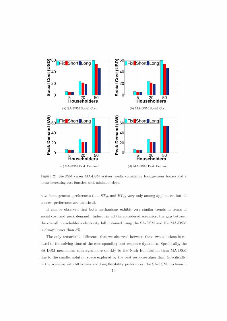
Figure 2: SA-DSM versus MA-DSM system results considering homogeneous houses and a

linear increasing cost function with minimum slope.

have homogeneous preferences (i.e., STah and ETah vary only among appliances, but all

houses’ preferences are identical).

It can be observed that both mechanisms exhibit very similar trends in terms of

social cost and peak demand. Indeed, in all the considered scenarios, the gap between

the overall householder’s electricity bill obtained using the SA-DSM and the MA-DSM

is always lower than 3%.

The only remarkable difference that we observed between these two solutions is re-

lated to the solving time of the corresponding best response dynamics. Specifically, the

SA-DSM mechanism converges more quickly to the Nash Equilibrium than MA-DSM

due to the smaller solution space explored by the best response algorithm. Specifically,

in the scenario with 50 houses and long flexibility preferences, the SA-DSM mechanism

19

takes only 8 seconds, in average, to find the equilibrium, whereas the MA-DSM approach

needs around 15 minutes4. For this reason, the SA-DSM system can be considered an

excellent solution for scheduling the appliances execution, since it achieves practically

the same results of the MA-DSM system in terms of electricity bills and peak demand,

but in a remarkably lower time and with a fully distributed approach. As a consequence,

devices that individually take scheduling decisions represent an effective and efficient

solution for realistic Smart Grids deployments: only minimal computation and commu-

nication capacity is required among all system’s components, without any centralized

house controller.

It can be further observed from Figures 2(a) and 2(b) that, independently of the DSM

mechanism, users always benefit from higher scheduling flexibility. Indeed, larger execu-

tion intervals for shiftable appliances (i.e., the curves identified by “Long” in the figures)

always allow users to pay cheaper bills than those obtained with short and fixed flexibility

levels (i.e., curves identified by “Short” and “Fix”, respectively), since the DSM system

can explore a larger solution space. However, the cheaper bills obtained using the long

flexibility preferences come at the cost of longer solving time (i.e., the amount of time

required to find the Nash Equilibrium through the best response algorithm). Indeed,

we observed that the solving time of the long flexibility scenario doubles with respect

to the short flexibility case. Numerical results presented in Figures 2(a) and 2(b) also

show that the number of players marginally affects the gain that is achieved with the

proposed DSM systems. In particular, the electricity bill saving obtained with respect to

the no-flexibility scenario is around 11% and 22% for, respectively, the short-flexibility

and the long-flexibility scenarios, irrespective of the number of players and the DSM

mechanism. Indeed, while a larger set of players increases the competition, the pro-

posed DSM mechanisms achieve the same gains by efficiently exploiting the flexibility of

shiftable appliances.

One of the main advantages for the operator to adopt the proposed SA-DSM system,

as illustrated in Figure 3, is that it automatically ensures the reduction of the electricity

demand during peak hours (i.e., high-price hours) without any centralized coordination

among users. Specifically, the peak demand decreases by as much as 22% using the SA-

4On an Intel Core i5 3.33 GHz, with a 4 GB RAM.

20

DSM system with respect to the value obtained considering fixed scheduling choices (i.e.,

the no-flexibility scenario), and the gain is slightly influenced by the appliances flexibility.

The reduction of the peak power demand results from shifting loads from peak hours to

other time-slots. To this end, only few users’ scheduling changes are required (i.e., only

appliances used at peak hours have to be shifted) and even a short flexibility can achieve

remarkable results.

0 4 8 12 16 20 240

5

10

15

20

25

30

Day Time (h)

Pow

er D

eman

d (k

W)

Fix Short Long

Fix vs Long: −22%

Fix vs Short: −21%

Figure 3: Peak reduction guaranteed by SA-DSM: aggregate power demand of 20 identical

houses (80 homogeneous appliances).

5.3. Analysis of Householder Preferences

Figures 4(a), 4(b) and 4(c) illustrate, respectively, the social cost, the peak demand

and the aggregated power profile of the proposed SA-DSM mechanism as a function of

the appliances flexibility. Specifically, these figures compare the results obtained with 20

homogeneous and heterogeneous houses.

As illustrated in Figure 4(a), the electricity bill is cheaper when considering het-

erogeneous players. Indeed, the power demand of heterogeneous houses can be more

smoothly distributed over the day than in the homogeneous scenario, due to the differ-

ent householders preferences about the time windows in which devices can operate. As

a consequence, since the energy price in every time slot is defined as a function of the

power demand of houses appliances in that particular slot, players can benefit from loads

spreading over time. Figure 4(b) shows that also the peak demand can be considerably

reduced when considering heterogeneous houses. Specifically, in this case, the proposed

21

Fix Short Long0

5

10

15

20

25

Devices Flexibility

Soc

ial C

ost (

US

D)

Homogeneous Heterogeneous

(a) Social Cost

Fix Short Long0

10

20

30

Devices Flexibility

Pea

k D

eman

d (k

W)

Homogeneous Heterogeneous

(b) Peak Demand

0 4 8 12 16 20 240

5

10

15

20

25

Day Time (h)

Pow

er D

eman

d (k

W)

Homogeneous Heterogeneous

−55%

(c) Power Profile

Figure 4: SA-DSM results with 20 homogeneous and heterogeneous houses preferences.

SA-DSM mechanism reduces the peak of the power demand down to 55% in the long

flexibility case with respect to the corresponding homogeneous scenario because of a

smoother load distribution. This effect appears clearly in Figure 4(c), where the overall

electricity demand over the 24 hours of 20 heterogeneous houses with loose scheduling

preferences (long flexibility) is compared to that of 20 identical residential houses.

5.4. Analysis of Energy Tariffs

To evaluate how energy tariffs affect the performance of the proposed DSM systems,

we fix the slope of the electricity pricing function s =0, 11 × 10−6

|20|e/kWh and we con-

sider four different tariff thresholds (i.e., the threshold on the aggregated demand above

which the electricity price becomes constant): πTT ∈ {15, 18, 21, 24} kW. Figures 5(a)

and 5(b) show the social cost and peak demand of a group of 20 identical houses as

a function of the devices flexibility considering the four aforementioned energy tariffs.

As expected, in all cases, the flexibility on the scheduling preferences reduces both the

electricity bill and the peak demand. However, by playing with the energy tariff, the

operator can further increase users’ gain on the electricity price and, at the same time,

decrease the peak power absorbed from the grid, thus resulting in lower investments

and operating costs. For example, as illustrated in Figure 5(a), the social cost decreases

down to 11% from the no-flexibility to the long flexibility scheduling scenarios when the

operator fixes the tariff threshold πTT = 15 kW. However, this gain increases up to 22%

with πTT = 24 kW. Indeed, when πTT = 15 kW, cost savings can be obtained only by

shifting loads from peak hours to time slots in which the total power demand is lower

than 15 kW. In contrast, a wider set of scheduling alternatives is available to reduce the22

Fix Short Long16

18

20

22

24

Devices Flexibility

Soc

ial C

ost (

US

D)

15 kW18 kW21 kW24 kW

(a) Social Cost

Fix Short Long20

22

24

26

28

Devices Flexibility

Pea

k D

eman

d (k

W)

15 kW18 kW21 kW24 kW

(b) Peak Demand

Figure 5: SA-DSM results with 20 identical houses and a varying tariff threshold (πTT ) of the

pricing function.

social cost when πTT = 24 kW, since power loads can be shifted from peak hours to all

time slots where the aggregated power demand is lower than 24 kW. As a consequence,

as the tariff threshold increases, the number of devices shifted outside the peak hours

grows, reducing the peak demand as illustrated in Figure 5(b).

In our tests, we also varied the slope s of the energy tariff to assess its impact on the

system performance. However, in the numerical results, which we do not show for the sake

of brevity, we observed no significant variation neither on the social cost nor on the peak

demand. Finally, we underline that in all the considered scenarios, we observed that all

players pay actually an equal share of the electricity bill, since the Jain’s Fairness Index

is always very close to 1. Indeed, even in the scenarios with heterogeneous residential

users, the JFI is always higher than 0.9991.

6. Conclusions

In this paper, we proposed a novel, fully distributed Demand-Side Management

(DSM) system aimed at reducing the peak demand of a group of residential users.

We modeled our system using a game theoretical approach, where players are the

customer’s appliances, which decide autonomously when to execute. We demonstrated

that the proposed game is a generalized ordinal potential one, and we proposed a best

response dynamics mechanism which is guaranteed to converge in few steps to efficient

23

Nash equilibrium solutions. Furthermore, we showed that our approach performs ex-

tremely close to a more complex setting where each customer must optimize the schedule

of all his appliances, since it provides practically the same results in terms of minimizing

their daily electricity bill. For this reason, due to its intrinsic simplicity, robustness and

distributed architecture, we recommend the adoption of our proposed approach.

Numerical results, obtained using realistic load profiles and appliance models, demon-

strate that the proposed DSM system represents a promising and very effective solution

to reduce the peak absorption of the entire system and the electricity bill of individual

customers in a fully distributed way.

Acknowledgment

This work was partially supported by the French ANR in the framework of the Green-

Dyspan project.

References

[1] European Commission et al. Europes energy position–markets & supply. Luxembourg: Publications

Office of the European Union, 2010.

[2] Justin Wilkes, Jacopo Moccia, et al. Wind in power 2010 european statistics. 2011.

[3] European Commission. European Union Energy in figures and factsheets, Sep. 2011. Available at:

http://ec.europa.eu/energy/publications/.

[4] M.A.A. Pedrasa, T.D. Spooner, and I.F. MacGill. Coordinated Scheduling of Residential Dis-

tributed Energy Resources to Optimize Smart Home Energy Services. IEEE Trans. Smart Grid,

1(2):134–143, 2010.

[5] X. Jiang, S. Dawson-Haggerty, P. Dutta, and D. Culler. Design and implementation of a high-

fidelity ac metering network. In IEEE Information Processing in Sensor Networks, pages 253–264,

2009.

[6] N. Bressan, L. Bazzaco, N. Bui, P. Casari, L. Vangelista, and M. Zorzi. The deployment of a smart

monitoring system using wireless sensor and actuator networks. In IEEE SmartGridComm, pages

49–54, 2010.

[7] C.W. Gellings and J.H. Chamberlin. Demand-side management: concepts and methods. The

Fairmont Press Inc., Lilburn, GA, 1987.

[8] T Joseph Lui, Warwick Stirling, and Henry O Marcy. Get smart. Power and Energy Magazine,

IEEE, 8(3):66–78, 2010.

24

[9] A. Mohsenian-Rad, V.W.S. Wong, J. Jatskevich, R. Schober, and A. Leon-Garcia. Autonomous

Demand-side Management Based on Game-theoretic Energy Consumption Scheduling for the Future

Smart Grid. IEEE Trans. Smart Grid, 1(3):320–331, 2010.

[10] Dov Monderer and Lloyd S. Shapley. Potential games. Games and Economic Behavior, 14(1):124–

143, 2012.

[11] G. Strbac. Demand side management: Benefits and challenges. Energy Policy, 36(12):4419–4426,

December 2008.

[12] M. Jacomino and M.H. Le. Robust energy planning in buildings with energy and comfort costs.

4OR - A Quaterly Journal of Operations Research, 10(1):81–103, 2012.

[13] A. Agnetis, G. Dellino, P. Detti, G. Innocenti, G. De Pascale, and A. Vicino. Appliance operation

scheduling for electricity consumption optimization. Decision and Control and European Control

Conference (CDC-ECC), 2011 50th IEEE Conference on, pages 5899–5904, 2011.

[14] Ana Soares, Allvaro Gomes, Carlos Henggeler Antunes, and Hugo Cardoso. Domestic load

scheduling using genetic algorithms. In Applications of Evolutionary Computation, pages 142–151.

Springer, 2013.

[15] Florian Allerding, Marc Premm, Pradyumn Kumar Shukla, and Hartmut Schmeck. Electrical

load management in smart homes using evolutionary algorithms. In Evolutionary Computation in

Combinatorial Optimization, pages 99–110. Springer, 2012.

[16] C. Clasters, T.H. Pham, F. Wurtz, and S. Bacha. Ancillary services and optimal household energy

management with photovoltaic production. Energy, 35(1):55–64, jul 2010.

[17] D. Livengood and R. Larson. The energy box: Locally automated optimal control of residential

electricity usage. Service Science, 1(1):1–16, 2009.

[18] Yuanxiong Guo, Miao Pan, and Yuguang Fang. Optimal power management of residential customers

in the smart grid. IEEE Transactions on Parallel and Distributed Systems, 23(9):1593–1606, 2012.

[19] A. Barbato, A. Capone, G. Carello, M. Delfanti, M. Merlo, and A. Zaminga. House energy demand

optimization in single and multi-user scenarios. In IEEE SmartGridComm, pages 345–350, 2011.

[20] A. Molderink, V. Bakker, M.G.C. Bosman, J.L. Hurink, and G.J.M. Smit. Domestic energy man-

agement methodology for optimizing efficiency in smart grids. In IEEE PowerTech, pages 1–7,

2009.

[21] C. Ibars, M. Navarro, and L. Giupponi. Distributed Demand Management in Smart Grid with a

Congestion Game. IEEE SmartGridComm, pages 495–500, October 2010.

[22] Micene project. Available on-line at http: // www. eerg. it/ index. php? p= Progetti_ -_ MICENE ,

2012.

[23] A. Barbato, A. Capone, L. Chen, F. Martignon, and S. Paris. A Power Scheduling Game for

Reducing the Peak Demand of Residential Users. IEEE Online GreenComm, October 2013.

[24] Daphne Geelen, Angle Reinders, and David Keyson. Empowering the end-user in smart grids:

Recommendations for the design of products and services. Energy Policy, 61(0):151 – 161, 2013.

[25] R. Jain. The Art of Computer Systems Performance Analysis: Techniques for Experimental Design,

Measurement, Simulation, and Modeling. Wiley - Interscience, 1991.

25