DDDAMS-based Real-time Assessment and Control of Electric ... · PDF fileDDDAMS-based...

1/36

DDDAMS-based Real-time Assessment and

Control of Electric-Microgrids

Nurcin Celik, PI

Team: Aristotelis E. Thanos, DeLante E. Moore, Xiaoran Shi

Simulation & Optimization Research Lab (SIMLab) Department of Industrial Engineering

University of Miami

DDDAS Program PI Meeting, Arlington, Virginia Sept, 2013

2/36 Outline

! Motivation ! Overview of the Proposed DDDAMS Framework

•  Measurements •  Decision-‐making algorithms •  Agent-‐based simulation of a microgrid •  Distributed generation sources •  Microgrid architectures and load types •  Cost analysis

! Experiments •  on 2-Tier IEEE-30 Bus System •  on 3-Tier IEEE-30 Bus System •  on Lab-scale Microgrid

! Results ! Conclusion and Future Work

3/36 Motivation

! USA and Canada, August 2003: Affected 55 million people

! Italy, September 2003: Affected 55 million people

! Java and Bali, August 2005: Affected 100 million people

! Brazil and Paraguay, November 2009: Affected 87 million people

! India, July 2012: Affected 670 million people

0

500

1000

1500

2000

2500

3000 Direct Effect Loss Earning

Indirect Effect Loss Earning

Industry and Residents

Government

Power Industry

Total Economic Impact

Economic Losses (in Billion $)

4/36 Motivation for the Air Force

§  Several questions arise in case of a power outage that affects an AF Base:

•  How should a real-time diagnosis and forensics analysis be performed automatically?

•  Was the root cause a technical incident or a power contingency? •  Did it occur because of an accidental failure or malicious and possibly ongoing attack?

•  A wide spread disturbance or just a localized outage of a few minutes?

•  How should the AFB microgrid respond to this abnormality (or catastrophe)?

•  What actions should be taken to secure the AFB power supply?

quick responsive and corrective actions are needed via autonomous control

5/36 Challenges in Power Dispatch

…about power networks

§  large # of variables, nonlinearities, and uncertainties §  operates at various scales §  resources =>more distributed §  generation =>more intermittent §  system =>more conducive to demand-response

…about dispatch control

§  changing demands §  very large range for the solution space §  Intense and time-‐critical information exchange §  significant burden on computational resources (processing of massive datasets)

6/36 Goal in Power Dispatch

•  To produce electricity •  Economically •  Environmentally friendly •  Reliably •  Securely

•  New dispatch methods are needed for robust and holistic system operations

Objective 1: Min Cost Objective 2: Min Emissions Constraints: Power Balance

Proposed Approach

•  Dynamic data driven adaptive multi-scale simulation

framework (DDDAMS) for efficient and reliable real-time

dispatching of electricity under uncertainty

7/36 Proposed DDDAMS Approach

§  Originates from the DDDAS paradigm that was first introduced by Darema (2000)

§  Investigates new algorithms and instrumentation methods for RT data acquisition and timely control of electricty microgrids in AF bases

§  Dynamically incorporates data into an executing application simulation

§  Dynamically steer the measurement process

§  More accurate analysis and prediction, more precise controls, and more reliable outcomes

§  Other application areas include

–  Natural disaster forecasting

–  Social and behavioral cognition

–  Biological system prediction

–  Supply chain management

–  Contaminant tracking…

8/36 Overview of Proposed DDDAMS Framework

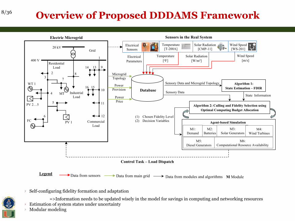
! Self-configuring fidelity formation and adaptation

=>Information needs to be updated wisely in the model for savings in computing and networking resources ! Estimation of system states under uncertainty ! Modular modeling

Sensory Data and Microgrid Topology

Database

Control Task – Load Dispatch

Power Price

Power Provision

Microgrid Topology

(1)  Chosen Fidelity Level (2)  Decision Variables

Electric Microgrid

Temperature [oF]

Electrical Parameters

Wind Speed [m/s]

Solar Radiation [W/m2]

Sensors in the Real System

Wind Speed [WS-201]

Temperature [T-200A]

Solar Radiation [CMP-11]

Electrical Sensors

Legend M Module Data from sensors Data from main grid Data from modules and algorithms

Industrial Load

Residential Load

Commercial Load

Grid 20 kV

WT 1

PV 2…5

PV 1

MT

400 V 1

2 3

4

5

6

7 8

9

10

11

12

13 14

15 16

FC

M2: Batteries

M3: Solar Generators

Algorithm 2: Culling and Fidelity Selection using Optimal Computing Budget Allocation

M1: Demand

Algorithm 1: State Estimation – FDIR

State Information Sensory Data

M6: Computational Resource Availability

M5: Diesel Generators

M4: Wind Turbines

Agent-based Simulation

9/36 Collection of Data from Various Sources

Database

Voltages, Current, Real and Reactive Power Injections

Power Systems Test Case Archive University of Washington

Sub-networks Split of the IEEE-30

Power Systems Literature Rakpenthai et al. 2005.

Atmospheric Science Data Center (NASA)/

Weather Underground Weather Profiles and Temperature

Wind Integration Datasets National Renewable Energy Laboratory (NREL)

Electrical Sensors

Wind Speed

CMP-11 Pyranometer

IEEE-30 Bus System Data

Solar Irradiance

Power generation/ Energy consumption from the AF, NREL, and EIA

• Tyndall AFB map • Energy consumption in the base • List of AF bases with renewables • Structure of the electricity network in base • Voltages and angles for buses • Power losses in branches • Apparent power for the transformers

§  Effective control of microgrid systems requires all-embracing acquisition of data about major system components

§  Fluctuating demand profiles, power generation (conventional /renewable), differences in power planning technologies, costs and availabilities of primary energy resources, transmission capacity etc.

AFB Site Visits

10/36 State Estimation Algorithm

Yes

No

START

END

New electrical measurement arrives

Store estimation of major states for

Correct the major state using the minor state estimation

Is interval over?

New environmental measurements arrive (i.e., temperature)

Estimate next major states using PF Subprocedure I

Estimate next minor state using PF Subprocedure II

State model for PF sub-procedure I:

Pk+1=aPk+u

Tk=bPk+1+v

a,b: calculated from historical data u: process noise v: measurement error

State model for PF sub-procedure I:

Pk+1=cPk+u

Zk=h(Pk+1)+v ∀j ∈ {1,2,…,m}

a,b: calculated from historical data h(.): function relating measurements to states u: process noise v: measurement error m: number of measurements within interval t

11/36 Particle Filtering

§  Represents probability densities by a set of randomly

chosen samples

§  Infers the posterior state given

§  transition prior

§  a realization of observations

§  Other application areas include…

•  Signal processing

•  Target tracking

•  Supply chain management

•  Optimization

Estimated Time-Dependent States

xt-1

xt

zt-1

zt

zt+1

Observations

t-1

t

t+1

p(zt|xt) Measurements depend only on state

Prior to xt

Posterior to xt

xt+1

x0 t=0

State Transition

Measurement

⋮

...........

...........

...........

...........

12/36

§  Purpose Set the level of detail in simulation for each pre-‐ deRined region (critical, priority and non-‐critical)

§  Goal •  Decrease the computational burden •  Increase the accuracy of decisions

§  Depends on •  Simulation model •  Optimal costing budget allocation (OCBA) scheme

§  Higher Ridelity means •  More frequent collection of data •  More frequent update to decision variables •  Shorter cycle time of dispatch update

Culling and Fidelity Selection Algorithm

Industrial Load

Residential Load

Commercial Load

Grid 20 kV

WT 1

PV 2…5

PV 1

MT

400 V 1

2 3

4

5

6

7 8

9

10

11

12

13 14

15 16

FC

Region 1

Region 2

Region 3

Fidelity 3

Fidelity 1

Fidelity 1

Fault detected

13/36 Agent-based System Simulation

14/36 Selection of Energy Sources via Userform

15/36 Overview of Agents Defined in Simulation

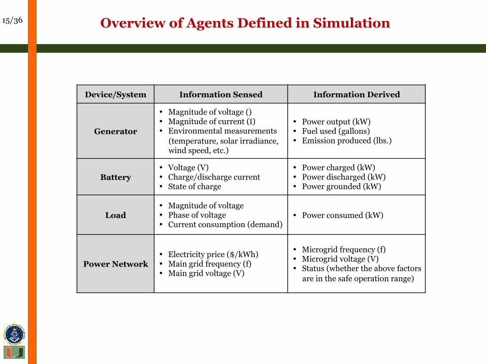
Device/System Information Sensed Information Derived

Generator

•  Magnitude of voltage () •  Magnitude of current (I) •  Environmental measurements

(temperature, solar irradiance, wind speed, etc.)

•  Power output (kW) •  Fuel used (gallons) •  Emission produced (lbs.)

Battery •  Voltage (V) •  Charge/discharge current •  State of charge

•  Power charged (kW) •  Power discharged (kW) •  Power grounded (kW)

Load •  Magnitude of voltage •  Phase of voltage •  Current consumption (demand)

•  Power consumed (kW)

Power Network •  Electricity price ($/kWh) •  Main grid frequency (f) •  Main grid voltage (V)

•  Microgrid frequency (f) •  Microgrid voltage (V) •  Status (whether the above factors

are in the safe operation range)

16/36 Renewable Generation via Solar Energy

§  Output •  Direct Current (DC source)

§  Major components •  PV array •  Battery storage unit •  Charge controller

§  Modeling techniques •  Analytical techniques

§  Cost •  Installation •  Maintenance

Direct solar irradiance

Indirect solar irradiance

(1)

(2)

(3)

Generation Transformation, Storage, Distribution

Consumption

1) Charge Controller, DC Power 2) Batter System , DC Power (3) Inverter, AC Power

§  Power output from a PV system with an area A(m2) when total solar radiation of Ir(kWh/m2) is

incident on PV surface, is given by

P=Ir.η.A

Where system efficiency η=ηm. .ηpc.Pf , module efficiency ηm=ηr.(1-β(Tc-Tr))

ηm. : manufacturer’s reported efficiency

ηpc : power conditioning efficiency

Pf : packing factor

β : array temperature coefficient

Tc : reference temperature for the cell efficiency

Tr : current temperature

17/36 Renewable Generation via Wind Energy

§  Output: DC , AC, Variable frequency AC sources (depending on the generator type)

§  Modeling techniques: Mathematical and dynamic model §  Cost: Installation and maintenance

§  A wind turbine generates electiricity only when the wind velocity V is within a standard range: Vmin≤ V ≤Vmax

§  Power output of a turbine with rated output Pr is:

P=0 V<Vmin P=aV3-‐bPr Vmin≤V<Vr P=Pr Vr≤V≤Vmax P=0 V>Vmax

Vr is the rated wind speed

a = Pr

Vr3 !Vmin3 b = Vmin

3

Vr3 !Vmin3

18/36 Renewable Generation via Ocean Energy

§  Output: AC •  A variable frequency AC source

§  Major components •  Wave Energy Device •  Power Cables •  Onshore Facility

§  Modeling techniques: State-of-the-art modeling and simulation

§  Avg. size: 1.9 square miles for utility scale system §  Cost: Installation and maintenance

Wave energy potential by location in MW/mile

§  Wind moves at higher speeds over water than over land

§  Wave action adds to the extractable surface energy

§  Major ocean currents (i.e., Gulf stream) may be exploited to extract energy with underwater rotors

§  Ideal locations for U.S. bases include Hawaii, Alaska, and Northern California

19/36 Fossil Fuel Energy

§  Output

•  Alternating Current (AC source)

§  Major components

•  Diesel engine •  Generator •  Ancillary devices (base, canopy, sound

attenuation, control systems, circuit breakers, jacket water heaters and starting system)

§  Modeling techniques: Analytical §  Cost: Purchase, Maintenance, Consumption

20/36 Various Microgrid Architectures

Utility Grid

Micro-grid Boundary

Load

Switching gear

Backup Generation

Renewable Energy

Utility Grid

Micro-grid Boundary

Load

Switching gear

Backup Generation

Renewable Energy

•  Backup generation can be used at any time •  Required Generators Mode:

ü  Isochronous Speed Control: when microgrid is isolated

ü  Droop Speed Control: when microgrid is served from utility grid (Diesel generation should align with utility grid frequency)

•  Backup generation can only be used when microgrid is isolated

•  Required Generator Mode: Isochronous Speed Control

ON/OFF EITHER/OR

21/36 Site Visit to Tyndall AFB in Florida

§  August 2013, SimLab visited Tyndall AFB, Civil Engineer Support Agency (AFCESA)

§  Base operating unit and host wing is 325th Fighter Wing of Air Combat Command (ACC)

§  Resides in a total area of 14.5 square miles

§  Total population: 2,932

§  Critical loads: Areas that directly impact national security, first responders and hospital

o  325 Fighter Wing HQ, AF North HQ

§  Priority loads: Command/control facilities for non-deployed U.S. based combat and supporting units

o  Actual squadrons, fighter, maintenance, and supporter groups

§  Non-critical loads:

o  Recreation, housing, and shopping areas

§  Ken Gray (Branch Chief, Renewable Energy) and Rexford Belleville P.E. (Electrical SME)

•  Toured the Tyndall Distribution network from substation to feeders •  Discussed current AF renewable energy projects •  Explained costs related to the power purchase agreements versus system purchases •  Discussed SPIDERS program and current military microgrid projects •  Emphasized fault detection portion of the framework for short term benefits

22/36 Cost Analysis (1)

23/36 Cost Analysis (2)

Solar System in Nellis AFB o  approximated total cost of $100,000,000 o  currently generating 30 GWh annually o  lifespan 20 years Cost : ~$ 0.167/KWh to purchase the system vs. ~$.0223/KWh via power purchase agreement vs. ~$.0715/KWh to purchase from Nevada Energy Cost of a utility scale system capable of meeting needs of an AF ~$2.79/W for solar ~$2.00/W for wind ~$4.57/W for ocean energy

§  AF budget is severely constrained for new projects for the next 10-‐20 years §  Private sector beneRits from tax beneRits and renewable energy credits §  Private sector has knowledge to operate and maintain utility scale power plants (AF would have to hire additional contractors to operate and maintain)

24/36 Experiments on 2-Tier IEEE 30 Bus System

Legend

Energy Load

Energy Generation

No Generation or Load

Bus

Line

Sub-network

2-Tier IEEE-30 Bus System ! 3 additional sources of DG at buses 7, 21, 23

=>Renewable/Nonrenewable

! Fidelities:

F1: Sub-network only

F2: Entire network

! Experiments are conducted on two separate

sets of scenarios on this network

1

2

3 4

5

6

7

8

9

10

11 12

13

14

15

16

17

18 19

20

21

22

24

25

27 28 29

30

8

26

23

2 5

132kV

132kV

132kV 132kV

132kV

132kV 132kV

132kV

132kV

1kV 33kV

33kV

11kV

11kV 33kV

33kV 33kV

33kV

33kV

33kV 33kV

33kV

33kV

33kV 33kV

33kV

33kV 33kV

33kV

33kV 21

23

7

25/36 Results: Scenario 1

! Set-up

§  Load variation may occur only within the sub-network

§  3%, 6% and 9% variations are studied

§  at Fidelity 1: Framework is run to optimize sub-network primarily

§  at Fidelity 2: Framework is run to optimize entire network

! Fidelity 1 reveals the best compromise solution

! Computational time reduced by 302 seconds

Fidelity 1

Load Variation

3% 6% 9%

Cost Range [600.59 -‐ 658.75] [608.39 -‐ 667.05] [605.61 -‐ 667.05]

Emissions Range [0.2672 -‐ 0.2673] [0.2672 -‐ 0.2673] [0.2672 -‐ 0.2673]

Compromise Cost 634.67 635.73 627.12

Compromise Emissions 0.26725 0.2673 0.26727

Fidelity 2 Load Variation

3% 6% 9%

Cost Range [524.28-‐697.35] [535.22 -‐ 693.58] [556.05 -‐ 721.85]

Emissions Range [0.2672-‐0.2674] [0.2672 -‐ 0.2674] [0.2671 -‐ 0.2674]

Compromise Cost 665.1 657.38 667.05


Load Variation Runtimes Fidelity 1 Fidelity 2 Savings in F1 (%)

3% 181.4516 483.5126 37.5278 6% 208.0058 471.3968 44.1254 9% 184.2011 652.9836 28.2091

26/36 Results: Scenario 1 (cont’d)

0.2672

0.2673

0.2674

0.2675

500 550 600 650 700 750 Emissions (Tons/h)

Cost ($/h)

Non-‐dominated Solution Set

Sub-‐Grid Optimizaion Full Optimization

0.26715 0.2672 0.26725 0.2673 0.26735 0.2674 0.26745

500 550 600 650 700 750

Emissions (Tons/h)

Cost ($/h)

0.26715 0.2672 0.26725 0.2673 0.26735 0.2674

500 550 600 650 700 750

Emissions (Tons/h)

Cost ($/h)

Best compromise

Loads 3% variated

Loads 6% variated

Loads 9% variated

! Fidelity 1 preferred solution


! Not necessarily overlapping

! If do overlaps, F1 is always beneficial from computational resource usage perspective

! Emission-results are to be detailed when renewables are introduced

Fidelity 1 Fidelity 2

27/36 Results: Scenario 2

! Set-up

§  Load variation may occur within the entire network

§  3%, 6% and 9% variations are studied

§  at Fidelity 1: Framework is run to optimize sub-network primarily

§  at Fidelity 2: Framework is run to optimize entire network

! Computational time reduced by 419 seconds

! However, very few of the solutions appear in the collective non dominated solution set

Fidelity 1 Load Variation 3% 6% 9%

Cost Range [601.39 -‐ 667.96] [605.73 -‐ 674.24] [646.47 -‐ 701.95]

Emissions Range [0.2672 -‐ 0.2673] [0.2672 -‐ 0.2673] [0.2671 -‐ 0.2672]

Compromise Cost 631.46 668.33 673.31


Fidelity 2 Load Variation 3% 6% 9%

Cost Range [560.07 -‐ 722.81] [572.36 -‐ 745.05] [588.72 -‐ 756.11]

Emissions Range [0.2671 -‐ 0.2674] [0.2671 -‐ 0.2673] [0.2671 -‐ 0.2673]

Compromise Cost 636.34 685.87 718.78


Load Variation Runtimes Fidelity 1 Fidelity 2 Savings in F1 (%)

3% 178.4844 536.2030 33.2867 6% 183.6092 663.1315 27.6882 9% 189.6595 609.3573 31.1245

28/36 Results: Scenario 2 (cont’d)

Loads are 3% variated



Best compromise

0.26715

0.26725

0.26735

550 600 650 700 750 Emissions (Tons/h)

Cost ($/h)

Non-‐dominated Solution Set Fidelity 1 Fidelity 2

0.2671

0.26715

0.2672

0.26725

0.2673

0.26735

550 600 650 700 750

Emissions (Tons/h)

Cost ($/h)

0.26705 0.2671 0.26715 0.2672 0.26725 0.2673 0.26735

550 600 650 700 750 Emissions (Tons/h)

Cost ($/h)



! Not necessarily overlapping

! If do overlaps, F1 is always beneficial from computational resource usage perspective

! Emission-results are to be detailed when renewables are introduced

29/24 Experiments on 3-Tier IEEE 30 Bus System

5

17

13

11

15

G

G

G G

G G

29

30

27

26 25

28

24

22

23

18 14

12

16

19

20 21

10

9

6

8

7

2

1 3

4

G

Sub-network 1

Sub-network 2

Sub-network 3 G

G G

LEGEND : Load G : Generation : No Generation or Load : Bus : Line

! IEEE-30 Bus System split into 3 sub-networks

! 5 additional sources of DG at buses 7, 21, 22, 23, 27

! 7 Fidelities via set of combination of sub-networks: 1,2,3,12,23,13,123

30/36

! Main framework is implemented in Matlab

! Simulations are run for 10 randomly generated cases of demand change

! Demand changes are rounded to the closest predefined scenario

! Fidelity selection algorithm chooses 2 different fidelities to simulate under selected scenario

! Validation process for algorithmic decisions

=>Simulate all fidelities under the selected scenario

=>Rank the best compromise solutions of the fidelities

!   Virtual Computing Facilities (CLOUD) at the UM

§  375 Intel 2.66 GHz CPUs cores §  1THz computational power §  1.5 TB RAM §  100 TB online storage §  720 Gbps of wire-speed ethernet switching §  1.2 Gbps firewall throughput §  60 TB backup tap library §  Compatibility testing §  Application troubleshooting

Experiments on 3-Tier IEEE 30 (cont’d)

31/24 Results: Comparison of Fidelity Selection

! In 8 out of 10 cases, best compromised solutions are within the 3 best fidelities under the predefined scenario

Case Load Variation (%)

Discovery Case Suggested Simulation 1 Suggested Simulation 2

Sub-‐Network 1 Sub-‐Network 2 Sub-‐Network 3 Sub-‐Networks Rank Sub-‐Networks Rank 1 0.39 1.50 1.32 0,0,0 1,3 4 2,3 3 2 0.99 0.54 3.77 0,0,5 2 1 1,3 5 3 0.32 2.74 2.27 0,5,0 1,3 2 2,3 3 4 3.90 1.69 0.39 5,0,0 1,2 7 3 6 5 2.26 0.10 2.60 0,0,5 2 4 1,3 1 6 2.55 4.56 6.70 5,5,5 1,2 7 2,3 2 7 5.74 3.48 1.38 5,5,0 1,3 3 2 6 8 7.40 0.45 2.28 5,0,0 1,2 6 3 5 9 4.50 3.45 12.39 5,5,10 3 5 2 3 10 10.36 6.24 4.26 10,5,5 1,3 3 1 2

32/24 Results: Comparison of Best Compromise Solutions

! Different, but how much?

! Worst case has shown a 3.38% difference in cost and 0.02% difference in emissions

Cases

Algorithm's Best Compromise Solution Global Best Compromise solution % Difference

Cost Emissions Cost Emissions Cost Emissions 1 594.29 0.2673 599.53 0.2673 0.87 0.01 2 613.29 0.2673 613.29 0.2673 0.00 0.00 3 615.64 0.2673 599.13 0.2673 2.76 0.01 4 599.29 0.2673 620.28 0.2672 3.38 0.02 5 598.19 0.2673 598.19 0.2673 0.00 0.00 6 569.41 0.2674 579.23 0.2673 1.70 0.01 7 569.68 0.2674 577.18 0.2673 1.30 0.00 8 573.53 0.2674 560.52 0.2674 2.32 0.00 9 597.7 0.2673 609.6 0.2673 1.95 0.01 10 534.86 0.2674 543.85 0.2674 1.65 0.01

33/36 Experiments with Hardware-‐in-‐the-‐loop: Lab-‐scale Microgrid

Lamp bulb

Simulates the function of a PV array

Controlled by a dimmer Represents the varying loads

Represents the inductive loads

Battery

DC motor

DC motor

Lamp bulb

Fan

Simulates the function of a diesel generator Power electronics (DC drives) for controlling the DC motors

Control of the switches

A lab-‐scale microgrid will allow for §  Highlighting of issues that are related to decision-‐making to control phase of DDDAMS §  Partial testing of different abnormalities in a real environment (even if its is in a simpler setting) §  Partial validation of the algorithms in our proposed framework §  Be familiar with potential challenges – problems in a microgrid

•  LabView: Handling of components of lab-microgrid •  Easypower: Running electrical model of Tyndall AFB •  Autocad: Examining electrical infrastructure of Tyndall AFB •  Anylogic: Agent based simulation of the considered microgrid •  JAVA: Implementation of algorithms and linkages to simulation •  Matlab: Implementation of algorithms

34/36 Conclusions

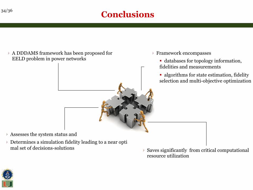
! Assesses the system status and

! Determines a simulation fidelity leading to a near optimal set of decisions-solutions

! A DDDAMS framework has been proposed for EELD problem in power networks

! Framework encompasses

§  databases for topology information, fidelities and measurements

§  algorithms for state estimation, fidelity selection and multi-objective optimization

! Saves significantly from critical computational resource utilization

35/36 Future Work

§  Algorithms: •  IdentiRication of uncertainties and extreme events for the Ridelity selection algorithm •  Improvements for algorithmic performance that will decrease computational burden

(while not foregoing accuracy) •  Incorporating isolation-desolation procedures •  Automatic fidelity generation via topology discovery

§  Simulation:

•  Incorporation of agents for additional power sources (microturbine, fuel cell etc.) •  Re-‐applying power balancing •  Aligning the framework algorithms (Ridelity selection, multiobjective optimization etc.) •  Additional user friendly forms for controlling the components of the simulation •  Conducting experiments for validation and testing

§  Additional Activities:

•  Establishing the lab-‐scale microgrid (collaboration with UM ECE for technicality) •  Conducting initial experiments with the lab-‐scale microgrid •  Upcoming site visits: Eglin AFB and MacDill AFB

36/36 Questions & Comments

This project is supported by the AFOSR via 2013 Young Investigator Research Award

(Award No: FA9550-13-1-0105)

DDDAMS-based Real-time Assessment and Control of Electric ... · PDF fileDDDAMS-based...

Documents

Transcript of DDDAMS-based Real-time Assessment and Control of Electric ... · PDF fileDDDAMS-based...