1001014 MILITARY TECHNICAL COLLEGE

911.1P ESEsEA S A Tr7-

DD -1 189

CAIRO - EGYPT

COMPUTATION OF ROBOT MANIPULATORS JACOBIAN :

A QUATERNION APPROACH

* A.S. ABDEL-MOHSEN

ABSTRACT

This work deals with the Jacobian computation for robot manipulators using a unified quaternion parameterization of position and orientation of members. Proposed generalized relations expressing the elements of manipulators Jacobian are derived in terms of Boolean parameters. These parameters introduce the contribution of both revolute and prismatic joints. The proposed relations are applied on a case study of a PUMA 560 robot manipulator for which analytical expressions of the Jacobian are obtained and tested by simulation.

I. INTRODUCTION

The major task of an industrial robot manipulator is to position and orient an end effector (EEF) during an approach phase of motion over a predefined time-based trajectory. To perform this task, a robot manipulator should have a mechanical structure of variable configuration with several powered joints between its members. In order to position and orient the EEF arbitrarily w.r.t a base fixed frame, the number of joints n or the degree of freedom of the manipulator must be greater than or equal to six. The first step in the formulation of the control problem of manipulators is to establish a relationship between the vector of EEF spatial coordinates X and the vector q of the joint coordinates or the general ized coordinates in the Lagrangian sense. The trajectory control of manipulators consists of forcing the vector X(t) to track a vector

Xd(t) representing the desired

evolution of the position and orientation of the EEF. A differential Inverse Kinematics Algorithm calculates the error Aq

of the joint variables corresponding to an error vector AX =

Xd(t) - X(t) to be compensated for. This process passes by the

* Associate Professor of Mechanical Engineering, Military Technical College, Cairo, EGYPT.

FIFTH ASAT CONFERENCE

4 - 6 May 1993, CAIRO

DD -1 190

computation of the manipulator Jacobian Matrix J(q). The

computation of the elements of X(t) and those of J(q) depends on

the kinematical parameterization of the manipulator. The computation of 3(q) for manipulators using the Homogeneous

Transformation Matrix parameterization is given in [1,2]. The use of Quaternions for the parameterization of manipulators has been recently investigated [4-9]. They provide a unified represent-ation of both position and orientation of members. In this paper, the computation of manipulators Jacobian in terms of quaternion parameterization is investigated. The organization of the paper is as follows : In section 2, the fundamental relations defining the unified quaternion position and orientation parameterization are shortly described. These relations are judged as essential for the derivation of the Jacobian matrix presented in section 3. The rest of the paper is reserved to the presentation of an application where a Quaternion based Jacobian of the PUMA 560 manipulator is obtained. A solution of the differential kinematic equations based on the Jacobian inversion is used to verify the validity of the obtained Jacobian by numerical simulation.

2. A UNIFIED QUATERNION PARAMETERIZATION OF POSITION & ORIENTATION

Consider a frame bF in a general space motion w.r.t. a frame nF.

Based on Chasle's theorem [3], the motion of bF w.r.t. nF is a

superposition of a translation following any point (say 01 ), the origin of bF, and a rotation about that point. This rotation may be defined by a Quaternion of Finite Rotation

en,b as [8,9],

en,b = cos(e/2) + sin(e/2)ii

(1)

where 9 and u are respectively the principal angle and the principal axis associated with Euler's theorem of finite rotation

[3]. The quaternion of finite rotation en,b is a unit quaternion

having the same representation on both frames bF and nF, i.e.,

en,b

* en,b 1 (2)

en b = b = [e 0

n n e

1 e2 e

3]t (3)

The four elements of the quaternion representation nfn,b are the

Euler parameters of finite rotation :

e0 = cos(0/2) el = ul sine/2))

(4) e2 = u2 sin(O/2) ; e

3 = u

3 sin(e/2)

FIFTH ASAT CONFERENCE DD -1 191

4 - 6 May 1993, CAIRO

The angular velocity of bF w.r.t.

nF may be expressed as [5];

. * nec n 2n -241,b —n,b

(5)

The position of bF w.r.t.

nF is defined by the vector quaternion

Pn,b from the origin On

of nF to the origin 0b of bF. Pn,b

and

its representation are expressed as :

Pn,b

- 0 +n0b

- n[0 x y z]t nEn,b

where x,y and z are the coordinates of 0b in

nF.

Vector Transformations - Successive Rotations :

Consider a spatial quaternion vector V. It may be shown [9] that

the representations of V w.r.t. bF and

nF are related by

* bV * nec nV ne (7)

—n,b

Eq.(7) is the quaternion equivalent of Vector Transformations.

Consider three frames 1F, mF and

nF in successive rotations; it may be shown [9] that when the quaternions of finite rotations are represented w.r.t. local frames, the representation of the overall rotation corresponds to the post multiplication of the quaternion for the fore rotation by that for the following rotation i.e.,

1!1,n -

11,m *

mem,n ( 8) —

Manipulator Kinematics

A robot manipulator is considered here as an open kinematic chain of rigid links. The first link is fixed to the base frame and the last link is attached to an end effector. The links are numbered starting from the base link which is given the number O. The last link is given the number n which is the degree of freedom of the manipulator, A right handed orthogonal frame

iF is assigned to each link i

according to Denavit & Hartenberg convention [2]. iF may be

obtained starting from i-1F through four steps of successive

rotations and translations as follows : a) Rotation around the zi_l atanangleei;b) Translation in the direction of x by

the member length ai ; c) Translation in the direction of z1-1 by

di; d) Rotation about xi by the member twist ai.

Based on Eq.(8), the orientation of iF w.r.t. I-1F is given by,

(6)

FIFTH ASAT CONFERENCE

4 - 6 May 1993, CAIRO

DD -1 192

1-1 =1-1(0 ) *

a

where

1-1 ni-1,a(01) = [cose1 /2 0 0 sine /2] ;

ae a .(a.) = [cosa

1 /2 sinai/2 0 0] ; -, 11

i-1e. -1-1,i

=

cos

cos

sin

sin

6 1/2 61/2

6 1/2

91/2

cos

sin

sin

cos

ai/2

ai/2

ai/2

ai/2

The position of 1F w.r.t. 1-1F may be specified by 1-1

E1-11 = [0 a1 cos e i 1 d ]t (11) a1 sin ei d1

]t

a revolute joint, the joint variable qi - ei while for a prismatic joint qi = di.

Based on Eq.(8) the orientation of link 1 w.r.t. link j(j<i) is,

The position of linkA w.r.t. link j may, however, be defined by the position vector P

Ji from .0.

3 to 0

1 represented in 3F as

(9)

(10)

je - Je * j+1 -.Li -3,3+1 S-j+1,j+2

*....* 1-le (12)

j k-j+1 ,k-1

* k-1p -k-1,k

* jec -j,k -1 (13)

For a manipulator having n links, the position and orientation of

the EEF w.r.t, the base frame are given respectively by PO,n and e

. Their representations in the base frame are expressed using 0,n Eqs.(12) and (13) as :

n Op v 0 ±-1Ei-1,i *

0 c t * X Y Z] (14) =0 n = 4" f-O i-1 f-0,1-1 = [0 ' 1=1 '

e0,n = 0 0 1 1 2 *...* e * 1e n-1 c

2n-1,n = [E0 E1 E

2 E3]

t (15) -, ,

The elements of 0 P 0 0,n - and e0 n are grouped in a vector X : - -,

X [X1 X 2]

t (16)

n -1 q i

3(2 X2 1

n q E

1=1 = E aqa

i°1 i (20-b)

FIFTH ASAT CONFERENCE DD -1 193

4 - 6 May 1993, CAIRO

where X1 - M oP0,n = [X Y Z]t (17)

X 0e-0 E 2 0 E1 ,n = [E0 E 3]t

(18)

I3' ]- and I3 is a 3x3 unit matrix

The vector X(7x1) hence defines uniquely the position and orientation of the EEF w.r.t. the base frame. It should however be noted that the last four elements of X are not independent. They are inter-related by the normality condition (Eq.(2)). The right hand side of Eqs.(17) and (18) are function of the manip lator configuration defined by the vector q.

manipulator using quaternion parameterization and may be rewritten as ;

X - X(q) (19)

3. QUATERNION-BASED JACOBIAN COMPUTATION

The differentiation of Eq.(19) w.r.t. time yields n

k = E (x) 1=1

o

0

ci i

Or :

(20-a)

Eq.(20-b) may be rewritten in the following matrix form

1 22 2n •

k2

(,20-c)

where Je is a 7xn jacobian matrix which relates the motion rate

of the EEF X to the joint speeds CI: The upper 3x1 portion of the ith column of J

e is associated with

position of the EEF and is given by :

P = P + 0P 1 0: ( L0P —0,n] 4 (0 -0,1-1 -1-1,n) -

1 1 (21-a)

The analysis of Eqs.(10-13) shows that Oq 0 (OP -0,1-1)-0. Eq.(21-a),

hence, reduces to,

a (0 0 )

0 1-1 Oc (21-b) i -, qi(-, * E1-1,n e0,1-1)

The analysis of Eqs.(10-13) shows also that

DD -1 194

ij _ 0 (0

!0,1-1) 0 roe .

t. 0,1 Oq

However;

FIFTH ASAT CONFERENCE

4 - 6 May 1993, CAIRO

CP = 0 Oq i,n (22)

(23)

(24)

0. 0 ri-1

Ei-lin) 0(4 0 (i-1 P. Oqi -1-1,i +

qri-1e *p e i-1c O i -1-1,i -i,n -i-1,i)

For a prismatic joint and based on Eq.(11),

(i.-1P-1,i) = [0 0 0 lit = i-1k-1 Oqi

Using Eq.(22) it may be shown that

*p * i-1 C 0 (i-1 ( ) 25 Oqi -i,n = 0

Substituting from Eqs.(22-25) into (21-b), pi for a prjsmatic

joint is expressed as :

Pi = 0e . 1-1k e * 0c . (26) -1 -0,1-1 1-1 -0,1-1

For a revolute joint and based on Eq.(11),

(i-1 Oqi pi-1,i -ai sin q1 a1 cos q1 0]t (27)

Considering on the other hand the quaternion product it may be shown that :

1-1k * i-1P-asilaq.a_cosq.0]t (28) ri 1 1-1 1 1 1 1

and based on Eqs (9,10) it may also be shown that :

0 ri-12i_iri) = 12 riki_, * 1-1 agil 2 (29-a) 1-1,1);

a i-lec 1 _ 12 (i-127-1,1 * i-lki_i) (29-b) '3(10- -1-1,ij

Based on Eqs.(22) and (29) the last term in the R.H.S. of Eq.(23) may be rewritten as :

a [1-1e * i p e 1-1c

Oqi -1-1,1 -i,n -1-1,i

0 (i-1e * i-1 c Oqi ) * ip -1,n

+

1-1 * 1p * 0 r e ) 1-lC 2i-1,1 -i,n dq 1

(30-a)

1

DD -111951 FIFTH ASAT CONFERENCE

4 - 6 May 1993, CAIRO

0 [1.-1e. * p * 1-1 c Oqi -1-1,1 -i,n

e. -1-1,1)

1 (i-1k i-1e * p 1-1 C )

! 2 1-1 -1-1,1 -1,n i-1,i

11 e 1-1 * e ip * 1-1 * c 1-1k (30-b) 2 i -i-1,i -i,n -i-1,i 1-1)

1 (1-1k iP. ) + 1 (1P * i-lk 1 *

(30-c)

- 2 l 1-1 -1,n 2 -1,n 1-1J

Substituting from eqs.(22,23,27,28 and 30-c) into (21-b), p1 for

a revolute joint is expressed as;

_. _ 140e i-1k i-1 * 0ec * * P (31)

El -0,i-1 i-1 -1-1,n -0,1-1]

Based on Eqs.(26) and (31), a generalized expression for the position portion of the Jacobian matrix is given by,

pi= Mr!0,1-1* (1-°.i) f i-1 k *0ec

1-lei i-lki-l*i-lE1-1,n) -0,1-11 (32)

WhereceiisaBoolearlIparameter,a.1 m0 for a prismatic joint and

ai = 1 for a.revolute joint.

, The lower 4x1 portion of the ith column of Je

is associated with

the orientation of the EEF and is given by,

(0e 0 0 ri-1 * ie

h .- (33-a)

1 eqi -0,n) - !0,1-1

* Oqii 21-1,1) -1,n

Using the results of Eq.(29), Eq.(33-a) reduces to

1 CD e 1-1k i-1 *

i-1 *

(33-b) h1 - 2 -0,1-1 !1-1,n)

for joint 1 being a revolute joint and;

h1 0 (33-c)

for joint 1 being a prismatic joint. A generalized expression for hi may hence be written as :

1 fo * 1-1k i-1 * i-1

hi = (34)

2 ("IA 2.0,1-1 -2.1-1,n)

Equations (32) and (34) express in general the elements of Je

which is defined by Eq.(20-c). It should be noted that the left hand side of Eq.(20-c) is a 7x1 vector X consisting of two parts:

1) the upper 3x1 vector Xi - v representing the components of the

Oec -0,n

= n

1-• i1

H "11.

= 2 r 0 ro facI , L 1=1

(35)

I

DD -111961 FIFTH ASAT CONFERENCE

4 - 6 May 1993, CAIRO

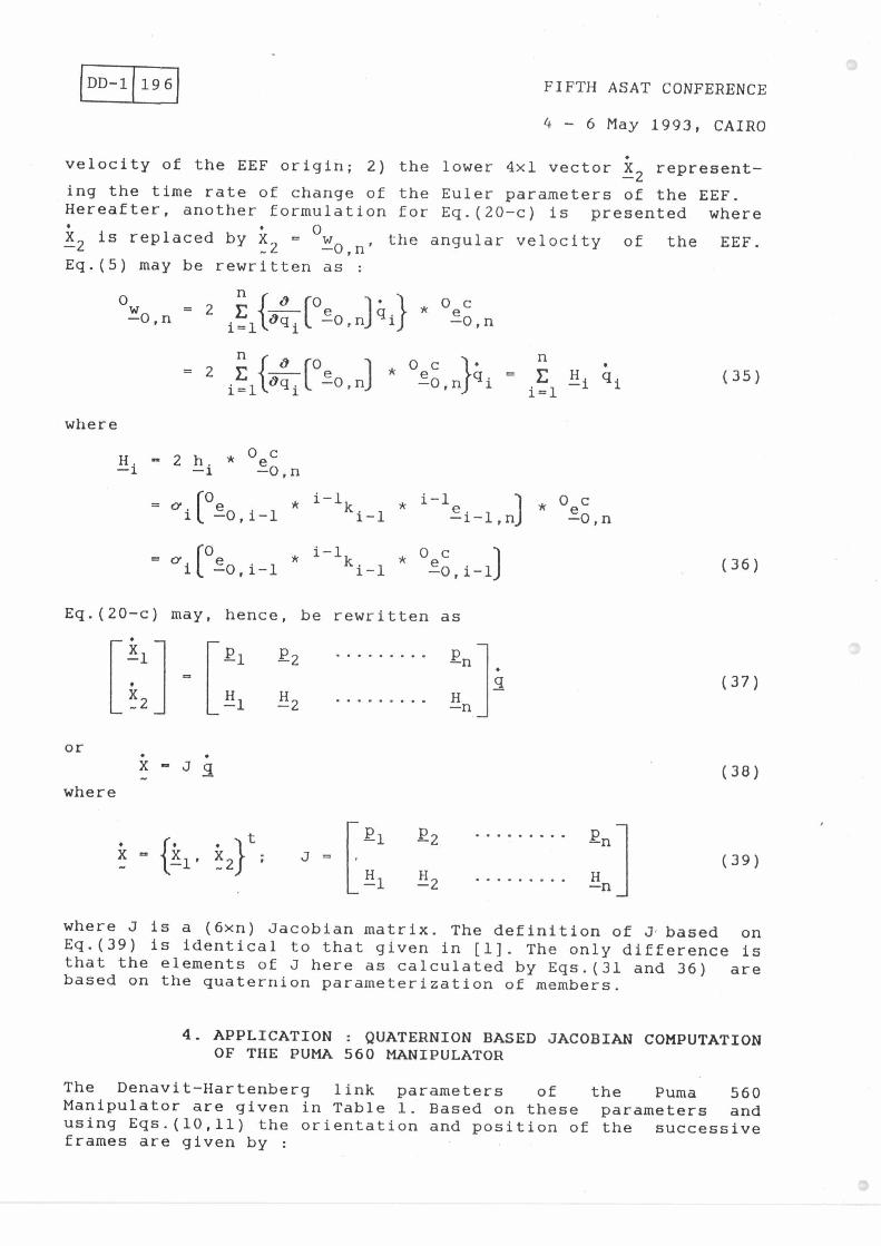
velocity of the EEF origin; 2) the lower 4x1 vector X2 represent-

ing the time rate of change of the Euler parameters of the EEF. Hereafter, another formulation for Eq.(20-c) is presented where

• X2 is replaced by X2 = °w0 n' the angular velocity of the EEF.

Eq.(5) may be rewritten as :

n foo 0w 0 c -0,n = 2 Oqi( f-0,ni *

where

H i - 2 hi 0ec

-1 -0,n

= a.10e i-1k. i-1e. 1 * oec -0,i-1 1-1 -1-1,nj -0,n

= a (

0e , i-1k. * 0 ec . ) -0,1-1 * 1-1 -0,1-1

Eq.(20-c) may, hence, be rewritten as

(36)

El 22 2n (37)

-H1 -H2 -Hn

X e J q (38) where

X = fk k2 J =

P1 22 2n

1 E2 - n

(39)

where J is a (6xn) Jacobian matrix. The definition of J based on Eq.(39) is identical to that given in [1]. The only difference is that the elements of J here as calculated by Eqs.(31 and 36) are based on the quaternion parameterization of members.

4. APPLICATION : QUATERNION BASED JACOBIAN COMPUTATION OF THE PUMA 560 MANIPULATOR

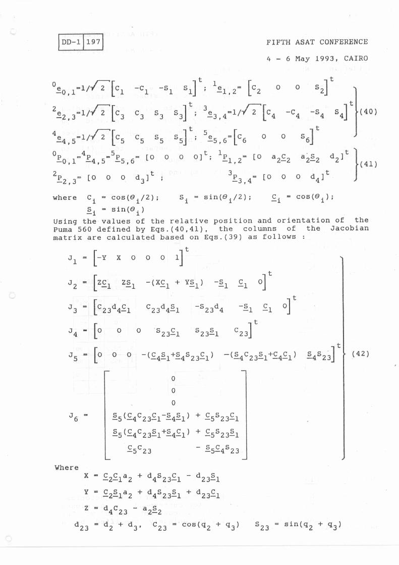
The Denavit-Hartenberg link parameters of the Puma 560 Manipulator are given in Table 1. Based on these parameters and using Eqs.(10,11) the orientation and position of the successive frames are given by :

Al —

2

or

FIFTH ASAT CONFERENCE DD -1 197

4 - 6 May 1993, CAIRO

t t oe0,1-1/121c1 -C1 -Si Sl] ; 1.21,2= [C2 0 0 S2]

t t 2e2,3-1/1121C3 C3 S3 S3] ;

3e3,4 1/1 21C4 -C4 -S4 S4] (40)

t t 4e4,5-1/1-2105 C5 S5 S5] ;

5.2.5,64C6 0 0 S6]

0 t P -4P -5P = [0 0 0 01t 1, [0 a2C2 d2 0,1 4,5 5,6 ' ; '1,2--

2P2,3 -, [0 0 0 d3 ' ]t • 3.,E.3,4- [0 0 0 d4]t

where C cos(ei/2); Si = sin(ei/2); Ei - cos(e); Si sin(ei)

Using the values of the relative position and orientation of the Puma 560 defined by Eqs.(40,41), the columns of the Jacobian matrix are calculated based on Eqs.(39) as follows :

t J1 - [-Y X 0 0 0 1]

t J2 - [ZC1 ZS]. -(XCi + YS1) -S, Li 0]

J3 - [C23d4C1 C d 23 4-S 1 -S23d4 -S1 El

t J4 - [0 0 0 1E1 52351 1 C23]

J5 .., [0 0 0 -(E4E1+E4S23E1) -(S C C ) S S 4 231S+ 4-C 1 -4 23

0

0

0

E5(E4c23E1-14E1) E552321

E5(E4C23E1+E4E1) + E5523E1

E5C23 - E5E4523

Where

-2-1 2 CCa + d4S23 C1 - d23S1

Y=CSa +dS S +d -2-1 2 4 23-1 23-C 1

Z = d4C23 - a2S2

J6

k (42)

d23 = d2 + d3, C23 = cos(q2 + q3) S23 = sin(q2 + q3)

FIFTH ASAT CONFERENCE DD-1 198

4 - 6 May 1993, CAIRO

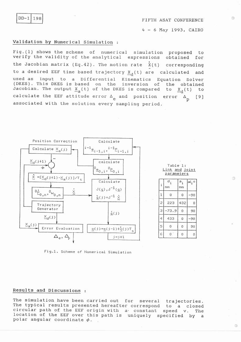
Validation by Numerical Simulation :

Fig.(1) shows the scheme of numerical simulation proposed to verify the validity of the analytical expressions obtained for

the Jacobian matrix (Eq.42). The motion rate X(t) corresponding

to a desired EEF time based trajectory Xd(t) are calculated and

used as input to a Differential Kinematics Equation Solver (DKES). This DKES is based on the inversion of the obtained Jacobian. The output Xa(t) of the DKES is compared to Xd(t) to

calculate the EEF attitude error Ae and position error A [9]

associated with the solution every sampling period.

Position Correction

Calculate

i-1 —i-1,i' —1-1 i

Calculate X 0) a

Xd (j+1)

calculate

0 Op

-0,i' -0,i

X =EXd(j+1)-Xa(j)1/Ts

Calculate

J(a),J-1(a)

20)=J-1

0. 0w —0,n' 0,n

Trajectory Generator

X ( d J)

X (j )

Error Evaluation

q(j)=q(j-1)+q(j)T

Ae,

j=j+1

Fig.1. Scheme of Numerical Simulation

Table 1: Link and ioint parameters

1 di

MM

a1 .

mm

a.0

1 0 0 -90

2 223 432 0

3 -73.9 0 90

4 433 0 -90

5 0 0 90

6 0 0 0

Results and Discussions :

The simulation have been carried out for several trajectories. The typical results presented hereafter correspond to a closed circular path of the EEF origin with a, constant speed v. The location of the EEF over this path is uniquely specified by a polar angular coordinate 0.

FIFTH ASAT CONFERENCE

4 — 6 May 1993, CAIRO

DD-1 199

(DI x uri)dp

E- c Pia •uo 97

1 0

4 I I

0 °

ePortu) ap

C 0

13 II 0 IA O 4- O. \

•rs

111 S-W 0

ti

o• w

u 1l1

•-• W

(.9

01

L.

liltI I I I I 1 1 1

';1 .131gr. 1- ..,- SOdg ° 0000 o 0 0 0 0 0 d 0

0 0

0

-e-

0

0

U) N I 0

11 II II II

13 13 1> t> •

" 9! q N a.q f. 0 000000000

(00.0100 d v

130

-o w 4- Q1\ o. co 4-

o w ti

o c

u

w - 0

In

O

0 YY 1-

01

3▪ es

11 ML11 4-0

' • n 4- 4.. 0

C o

E • • •A0 O II > 0 W

01 •

O - 0

e E O N

• .1-• 0 3 II

0 O >

•-•

N 01

IL

1

DD -112001

0

6-

I I m I ttir17'9!MNm 41.M17 0 00 0660600

0

7:24,U) 47

0

I,• 0 r0 n\ a, _Ju

C4- MN ,

O O /- 100

I-

-W 0 C

4, 0

1' 4_ 01 4_0 wa

C

117 01

4- OM

4+7 y.

C .0 0

117

01

01 C

11-•

aI D II C4- MN. .04- o 11)- /00

4_41 0

13 117

to-v

C no

tL

FIFTH ASAT CONFERENCE

4 - 6 May 1993, CAIRO

8

I I • 4 I

•a v

0

I I 0 ,$1

N0U01,17 cf 0

MN 134-1 a 11

CN /0

O >- 0 0

o c

O

v-

• V

1

WO-

C 111 0

8

1111 111111II1111;11 0 ^ Np0 tt 6. 117 ". 66 is ""4 * 11 17 0 6 6 o 6 6 6 06

[00,•Ig a v

FIFTH ASAT CONFERENCE

4 - 6 May 1993, CAIRO

DD -1 201

Figs.(2.a,b) show respectively the evolution of position and attitude errors for two successive turnes of the EEF over the

circular path with a reference speed v = vo = 0.2 m/s. The

Jacobian here is updated every computation step. It can be seen that both errors are bounded (this is due to the effect of the position correction loop used). The of magnitude of errors are Ae 5 0.3 m.rad. and A -5. 0.1 pm.

Figs.(3.a,b) represent the evolution of errors for different values of speed v as indicated by the dimensionless parameter v - v/vo

. Both errors are again bounded, however, the order of

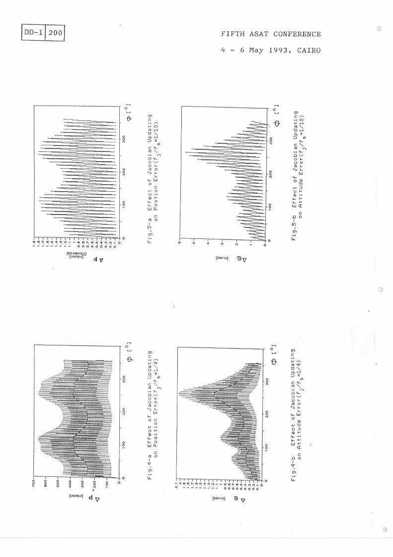
magnitude of errors increases as v increases. The main disadvantage of using a DKES based on the Jacobian inversion is the computation effort associated with the matrix inversion. To overcome this problem, one may reduce the Jacobian updating frequency f3 w.r.t. the solution frequency fs

. The

effect of fj on the solution accuracy may be seen from the

comparison of Figs.(4-a,b) and Figs.(5-a,b). Both are calculated for v - 0.5 and for f

1 /f respectively equal to 1/4 and 1/10. It

canberecognizedthatasf.3 decreases Ap and A increase. A

compromise between the computation effort and the solution accuracy may be achieved by a proper selection of f.

3.

CONCLUSION

Quaternions establish a unified representation and a symmetric treatment of manipulators members position and orientation. Proposed generalized relations expressing the elements of manipulators Jacobian based on quaternion parameter- izations are derived. The study of these relations shows that they have the same physical meaning as those derived on basis of Homogeneous Transformation parameterization [1]. Using the derived relations the Jacobian matrix for the Puma 560 manipulator is obtained and tested by numerical simulation. The test results are quite satisfactory. Proper selection of the frequency of Jacobian updating enables one to reduce the computation burden associated with the Jacobian inversion keeping the level of the solution accuracy.

REFERENCES

1. PAUL R.P. (1981) "Robot Manipulators : Mathematics, Programm-ing and Control", Cambridge, MA : MIT Press.

2. Fu K.S., Gonzalez R.C., Lee C.S.G., (1987) "ROBOTICS : Control Sensing, Vision and Intelligence" McGraw-Hill.

3. Ginsberg J.H. (1988) "Advanced Engineering Dynamics" HARPER & ROW, Publishers, New York.

4. Spring K.W., (1986), "Euler Parameters and the Use of Quater-nion Algebra in the Manipulation of Finite Rotations : A Review" Mechanisms and Machine Theory, Vol.21, No.5, pp 365-373.

5. Lin S.K. (1988), "Euler Parameters in Robot Cartesian Control" Proc. of IEEE Int. Conf. on Robotics and Automation.

FIFTH ASAT CONFERENCE DD -1 202

4 - 6 May 1993, CAIRO

6. Chou J.C.K., Kamel M. (1988), "Quaternion Approach to Solve Kinematic Equation of Rotation, AA

x AxAb,

of a Sensor-

Mounted Robotic Manipulator", proc. of the IEEE Int. Conf. on Robotics.

7. Funda J., Paul R.P. (1988), "A Comparison of Transformation and Quaternion in Robotics", proc. of the IEEE Int. Conf. on Robotics.

8. Abdel-Mohsen A.S. (1991), "Quaternion Based Kinematics of Robot Manipulators" 6th International Conference on CAD/CAM, ROBOTICS & FOF, South Bank Polytechnic, London, August 19-22, 1991.

9. Abdel Mohsen, A.S. (1992), "On the Use of Euler' Parameters in Robotics : Theory and Application", Proceedings of the 5th AME conference, Military Technical College, Cairo,. May 5-7, 1992.

ABBREVIATION AND NOTATION

EEF End Effector DKES Differential Kinematic Equation Solver

Denotes a quaternion product Head Symbols : : Quaternion

-* : Vector Bottom notation - : 4x1 column which correspond to the represent-ation of a quaternion in a given frame. Left superscript denotes the basis or the frame w.r.t which a quaternion representation is considered. Right superscript c denotes the conjugate of a quaternion or its representation.

Right Subscript under a quaternion of rotation denotes the direction of rotation.