LECTURE NOTES

ON

DC MACHINES

(17CA02301)

2018 – 2019

II B. Tech I Semester (CREC-R17)

Mr. K.Raju, Assistant Professor

CHADALAWADA RAMANAMMA ENGINEERING COLLEGE (AUTONOMOUS)

Chadalawada Nagar, Renigunta Road, Tirupati – 517 506

Department of Electrical and Electronics Engineering

JAWAHARLAL NEHRU TECHNOLOGICAL UNIVERSITY ANANTAPUR

DC MACHINES

III Semester: EEE

Course Code Category Hours / Week Credits Maximum

Marks

17CA02301 Core L T P C CIA SEE

Tota

l

2 2 - 3 30 70 100

Contact Classes: 34 Tutorial Classes: 34 Practical Classes: Nil Total Classes: 68

OBJECTIVES:

To make the students learn about:

I. The constructional features of DC machines and different types of winding employed in

DC machines

II. The phenomena of armature reaction and commutation

III. Characteristics of generators and parallel operation of generators

IV. Methods for speed control of DC motors and applications of DC motors

V. Various types of losses that occur in DC machines and how to calculate efficiency

VI. Testing of DC motors

UNIT-I PRINCIPLES OF ELECTROMECHANICAL ENERGY

CONVERSION Classes: 12

Sources of dc Supply- Electromechanical Energy Conversion – Forces and Torque In Magnetic

Field Systems – Energy Balance – Energy and Force in a Singly Excited Magnetic Field System,

Determination of Magnetic Force - Co-Energy – Multi Excited Magnetic Field Systems.

UNIT-II D.C. GENERATORS –I Classes: 14

D.C. Generators – Principle of Operation – Constructional Features – Armature Windings – Lap

and Wave Windings – Simplex and Multiplex Windings – Use of Laminated Armature – E. M.F

Equation– Numerical Problems – Parallel Paths-Armature Reaction – Cross Magnetizing and

De-Magnetizing AT/Pole – Compensating Winding – Commutation – Reactance Voltage –

Methods of Improving Commutation.

UNIT-III D.C GENERATORS – II Classes: 14

Methods of Excitation – Separately Excited and Self Excited Generators – Build-Up of E.M.F -

Critical Field Resistance and Critical Speed - Causes for Failure to Self-Excite and Remedial

Measures-Load Characteristics of Shunt, Series and Compound Generators – Parallel Operation

of D.C Series Generators – Use of Equalizer Bar and Cross Connection of Field Windings –

Load Sharing- Applications of DC generators.

UNIT-IV D.C. MOTORS Classes: 14

D.C Motors – Principle of Operation – Back E.M.F.– Circuit Model – Torque Equation –

Characteristics and Application of Shunt, Series and Compound Motors – Armature Reaction

and Commutation.Speed Control of D.C. Motors: Armature Voltage and Field Flux Control

Methods. Ward-Leonard System–Braking of D.C Motors – Permanent Magnet D.C Motor

(PMDC). Motor Starters (3 Point and 4 Point Starters) – Protective Devices-Calculation of

Starter Steps for D.C Shunt Motors.

UNIT-V TESTING OF DC MACHINES Classes: 14

Losses – Constant & Variable Losses – Calculation of Efficiency – Condition for Maximum

Efficiency. Methods of Testing – Direct, Indirect – Brake Test – Swinburne’s Test –

Hopkinson’s Test – Field’s Test – Retardation Test- Applications of DC Motors.

Text Books:

1. Electric Machines by I.J. Nagrath & D.P. Kothari, Tata Mc Graw – Hill Publishers, 3rd

Edition, 2004.

2. Electrical Machines – P.S. Bimbhra., Khanna Publishers, 2011.

Reference Books:

1. Performance and Design of D.C Machines – by Clayton & Hancock, BPB Publishers, 2004.

2. Electrical Machines -S.K. Battacharya, TMH Edn Pvt. Ltd., 3rd Edition, 2009.

3. Electric Machinary – A. E. Fitzgerald, C. Kingsley and S. Umans, Mc Graw-Hill Companies,

5th Editon, 2003.

4. Electrical Machines – M.V Deshpande, Wheeler Publishing, 2004.

5. Electromechanics – I - Kamakshaiah S., Overseas Publishers Pvt. Ltd, 3rd Edition, 2004.

Web References:

1. https://www.electrical4u.com/working-or-operating-principle-of-dc-motor

2. https://www.freevideolectures.com

3. https://www.ustudy.in › Electrical Machines

4. https://www.freeengineeringbooks.com

E-Text Books:

1. https://www.textbooksonline.tn.nic.in

2. https://www.freeengineeringbooks.com

3. https://www.eleccompengineering.files.wordpress.com

4. https://www.books.google.co.in

Course Outcomes: At the end of course, the student will be able to

Understand the construction and principle of working of DC Machines

Diagonise the failure of DC generator to build up voltage

Understand the gross torque and useful torque developed by DC motor

Understand the suitable methods and conditions for obtaining the required speed of DC

motor

Understand the Calculations of losses and efficiency of DC generators and motors

Over view of Applications of DC Machines.

UNIT I

Principles of Electromechanical

Energy Conversion Topics to cover:

1) Introduction 4) Force and Torque Calculation from

2) EMF in Electromechanical Systems Energy and Coenergy

3) Force and Torque on a Conductor 5) Model of Electromechanical Systems Introduction

For energy conversion between electrical and mechanical forms, electromechanical

devices are developed. In general, electromechanical energy conversion devices can be

divided into three categories:

(1) Transducers (for measurement and control)

These devices transform the signals of different forms. Examples are microphones,

pickups, and speakers.

(2) Force producing devices (linear motion devices)

These type of devices produce forces mostly for linear motion drives, such as relays,

solenoids (linear actuators), and electromagnets.

(3) Continuous energy conversion equipment

These devices operate in rotating mode. A device would be known as a generator if

it convert mechanical energy into electrical energy, or as a motor if it does the other

way around (from electrical to mechanical).

Since the permeability of ferromagnetic materials are much larger than the permittivity of

dielectric materials, it is more advantageous to use electromagnetic field as the medium for

electromechanical energy conversion. As illustrated in the following diagram, an

electromechanical system consists of an electrical subsystem (electric circuits such as

windings), a magnetic subsystem (magnetic field in the magnetic cores and airgaps), and a

mechanical subsystem (mechanically movable parts such as a plunger in a linear actuator and

a rotor in a rotating electrical machine). Voltages and currents are used to describe the

PRINCIPLES OFELECTROMECHANICAL ENERGY CONVERSION

UNIT-IPRINCIPLES OF ELECTROMECHANICAL ENERGY CONVERSION

Principle of Electromechanical Energy Conversion

state of the electrical subsystem and they are governed by the basic circuital laws: Ohm's

law, KCL and KVL. The state of the mechanical subsystem can be described in terms of

positions, velocities, and accelerations, and is governed by the Newton's laws. The magnetic

subsystem or magnetic field fits between the electrical and mechanical subsystems and acting

as a "ferry" in energy transform and conversion. The field quantities such as magnetic flux,

flux density, and field strength, are governed by the Maxwell's equations. When coupled with

an electric circuit, the magnetic flux interacting with the current in the circuit would produce

a force or torque on a mechanically movable part. On the other hand, the movement of the

moving part will could variation of the magnetic flux linking the electric circuit and induce

an electromotive force (emf) in the circuit. The product of the torque and speed (the

mechanical power) equals the active component of the product of the emf and current.

Therefore, the electrical energy and the mechanical energy are inter-converted via the

magnetic field.

Concept map of electromechanical system modeling

In this chapter, the methods for determining the induced emf in an electrical circuit and

force/torque experienced by a movable part will be discussed. The general concept of

electromechanical system modeling will also be illustrated by a singly excited rotating

system.

2

Principle of Electromechanical Energy Conversion Induced emf in Electromechanical Systems

The diagram below shows a conductor of length l placed in a uniform magnetic field of

flux density B. When the conductor moves at a speed v, the induced emf in the conductor can

be determined by

e lv B The direction of the emf can be determined by the "right hand rule" for cross

products. In a coil of N turns, the induced emf can be calculated by

e d

dt where is the flux linkage of the coil and the minus sign indicates that the induced current

opposes the variation of the field. It makes no difference whether the variation of the flux

linkage is a result of the field variation or coil movement.

In practice, it would convenient if we treat the emf as a voltage. The above express can

then be rewritten as

e d L di i dL dx dt dt dx dt

if the system is magnetically linear, i.e. the self inductance is independent of the current. It

should be noted that the self inductance is a function of the displacement x since there is a

moving part in the system. Example: Calculate the open circuit voltage between the brushes on a Faraday's disc as shown

schematically in the diagram below.

r

Shaft

r2 r1 - Brushes

B v SN SN

+

3

Principle of Electromechanical Energy Conversion

Solution:

Choose a small line segment of length dr at position r (r1rr2)from the center of the disc between the brushes. The induced emf in this elemental length is then

de Bvdr Br rdr

where v=rr. Therefore, r

2 r 2 r

r 2 r 2

2 r B

e de Br rdr r B 2 1

r1 2

r

2

1

Example: Sketch L(x) and calculate the induced emf in the excitation coil for a linear actuator

shown below. A singly excited linear actuator

Solution:

L x

N 2

Rg x

Rg x

2 g

and

o d xl

N 2 l d x

L x 2 g

o

e d

L di i dL dx

dt dt dx dt

di N 2 l

o

=L x dt i 2 g v

4

Principle of Electromechanical Energy Conversion

L(x)

L(0) O d X

Inductance vs. displacement

If i=Idc, N

2 l

e I dc o

v

2g

If i=Imsint, N

2 l

N

2 l

e o

d xI m cost vI m sint o

2 g 2 g

I m o N

2 l d x cost v sint

2 g

o N

2 l d x

2 2 v 2 v

I cos t arctan m

2 g d x

Force and Torque on a Current Carrying Conductor

The force on a moving particle of electric charge q in a magnetic field is given by the Lorentz's force law:

F qv B

The force acting on a current carrying conductor can be directly derived from

the equation as

F I Cdl B where C is the contour of the conductor. For a homogeneous conductor of length l carrying current I in a uniform magnetic field, the above expression can be reduced to

F I l B

In a rotating system, the torque about an axis can be calculated by T r F

where r is the radius vector from the axis towards the conductor.

5

Principle of Electromechanical Energy Conversion

Example:

Calculate the torque produced by the Faraday's disc if a dc current Idc flows from

the positive terminal to the negative terminal as shown below.

T

Shaft

r2 r1 - Brushes

B I SN SN

+

Solution: Choose a small segment of length dr at position r (r1rr2) between the brushes. The

force generated by this segment is dF Idrr$ Ba

z IBdra where a is the unit vector in direction. The corresponding torque is

dT r dF IBrdra z Therefore,

r 2 r

2

r2

IB 2 1 a

z

T dT IBrdra z 2

r1

Force and Torque Calculation from Energy and Coenergy A Singly Excited Linear Actuator

Consider a singly excited linear actuator as shown below. The winding resistance is R. At

a certain time instant t, we record that the terminal voltage applied to the excitation winding

is v, the excitation winding current i, the position of the movable plunger x, and the force

acting on the plunger F with the reference direction chosen in the positive direction of the x

axis, as shown in the diagram. After a time interval dt, we notice that the plunger has

6

Principle of Electromechanical Energy Conversion moved for a distance dx under the action of the force F. The mechanical done by the force acting on the

plunger during this time interval is thus

dWm Fdx The amount of electrical energy that has been

transferred into the magnetic field and converted into

the mechanical work during this time interval can be

calculated by subtracting the power loss dissipated in

the winding resistance from the total power fed into the excitation winding as

A singly excited linear actuator

dW dW dW vidt Ri 2 dt

e f m

Because e d v Ri dt

dWf dW

e dW

m eidt Fdx

we can write id Fdx

From the above equation, we know that the energy stored in the magnetic field is a function

of the flux linkage of the excitation winding and the position of the plunger. Mathematically,

we can also write

dWf , x W

f , x d

Wf

, x dx

x Therefore, by comparing the above two equations, we conclude

Wf , x Wf , x

i and F

x

From the knowledge of electromagnetics, the energy stored in a magnetic field can be expressed as

Wf , x i , xd 0

For a magnetically linear (with a constant permeability or a straight line magnetization curve

such that the inductance of the coil is independent of the excitation current) system, the

above expression becomes

7

Principle of Electromechanical Energy Conversion

Wf , x

1 2

2 L x

and the force acting on the plunger is then

Wf , x 1 2 dLx 1 dLx

F x 2 Lx dx 2 i 2 dx

In the diagram below, it is shown that the magnetic energy is equivalent to the area

above the magnetization or -i curve. Mathematically, if we define the area underneath the magnetization curve as the coenergy (which does not exist physically), i.e.

Wf ' i, x i Wf , x

we can obtain

Wf ( , x) ( , i)

dWf ' i, x di id dWf , x

di Fdx '

W ' i, x W ' i, x

Wf ( i, x )

f f

di

dx

i x

Therefore, O i

Wf ' i, x

Energy and coenergy

i

and F Wf ' i, x

x

From the above diagram, the coenergy or the area underneath the magnetization

curve can be calculated by i

Wf ' i, x i, xdi 0

For a magnetically linear system, the above expression becomes 1

Wf ' i, x 2 i 2 L x

and the force acting on the plunger is then

Wf ' i, x 1 i

2 dLx

F

x

dx

2

Example: Calculate the force acting on the plunger of a linear actuator discussed in this section.

8

Principle of Electromechanical Energy Conversion

R

g Ni

Rg

(c)

A singly excited linear actuator Solution: Assume the permeability of the magnetic core of the actuator is infinite, and hence the system

can be treated as magnetically linear. From the equivalent magnetic circuit of the actuator

shown in figure (c) above, one can readily find the self inductance of the excitation winding

as

L x N 2

o N

2 ld x

2 Rg 2 g

Therefore, the force acting on the plunger is

F 1 i 2 dL x

o l Ni

2

2 dx 4g

The minus sign of the force indicates that the direction of the force is to reduce the

displacement so as to reduce the reluctance of the air gaps. Since this force is caused by the

variation of magnetic reluctance of the magnetic circuit, it is known as the reluctance force. Singly Excited Rotating Actuator

The singly excited linear actuator mentioned above becomes a singly excited rotating

actuator if the linearly movable plunger is replaced by a rotor, as illustrated in the diagram

below. Through a derivation similar to that for a singly excited linear actuator, one can

readily obtain that the torque acting on the rotor can be expressed as the negative partial

derivative of the energy stored in the magnetic field against the angular displacement or as

the positive partial derivative of the coenergy against the angular displacement, as

summarized in the following table.

9

Principle of Electromechanical Energy Conversion

A singly excited rotating actuator Table: Torque in a singly excited rotating actuator

Energy Coenergy

In general,

dWf id Td dWf ' di Td

i

Wf , i,d Wf ' i, i,di

0 0

i

Wf ,

Wf ' i,

i

T Wf ,

T Wf ' i,

If the permeability is a constant,

W ,1 2 1 2

Wf ' i,

2 i L

2 2 L

1 dL

f

1 dL 1 dL

T

i2 T i 2

2 L d

2 d

2 d

Doubly Excited Rotating Actuator

The general principle for force and torque calculation discussed above is equally

applicable to multi-excited systems. Consider a doubly excited rotating actuator shown

schematically in the diagram below as an example. The differential energy and coenergy

functions can be derived as following:

dWf dWe

dWm where dWe e1i1dt e2 i2 dt

10

Principle of Electromechanical Energy Conversion

A doubly excited actuator

e d1 , e d2

dt

1 dt 2

and dWm Td

Hence,

dWf 1 , 2 , i1d1 i2 d2 Td

Wf 1 , 2 , Wf 1 , 2 ,

d1

d2

1 2

Wf 1 , 2 ,

d

and

dWf ' i1 ,i2 , di11 i2 2 Wf 1 , 2 ,

1di1 2 di2 Td

Wf ' i1 ,i2 , Wf ' i1 ,i2 ,

di1

di2

i1 i2

Wf ' i1 ,i2 ,

d

Therefore, comparing the corresponding differential terms, we obtain

T

Wf 1 , 2 ,

or T Wf ' i1 ,i2 ,

11

Principle of Electromechanical Energy Conversion

For magnetically linear systems, currents and flux linkages can be related by constant

inductances as following

1 L11 L12 i1

2 L

21 22 2 or

i1 11 121 2 21 22 2

where L12=L21, 11=L22/, 12=21=L12/, 22=L11/, and =L11L22L122

. The

magnetic energy and coenergy can then be expressed as

Wf 1 , 2 , 1 2

1 2

12 2 11 1 22 2 1

2 2

and

1 1

Wf 'i1 ,i2 ,

L i 2

2

2 2 L i L 12

i i 2

11 1 22 2 1

respectively, and it can be shown that they are equal.

Therefore, the torque acting on the rotor can be calculated as

Wf 1 , 2 , Wf ' i1 ,i2 ,

T

1 i 2

dL11 1 i 2

dL22 i i dL12

2 1 2

2 1 2

Because of the salient (not round) structure of the rotor, the self inductance of the stator is a

function of the rotor position and the first term on the right hand side of the above torque

expression is nonzero for that dL11/d0. Similarly, the second term on the right hand side

of the above torque express is nonzero because of the salient structure of the stator.

Therefore, these two terms are known as the reluctance torque component. The last term in

the torque expression, however, is only related to the relative position of the stator and rotor

and is independent of the shape of the stator and rotor poles.

Model of Electromechanical Systems

To illustrate the general principle for modeling of an electromechanical system, we still

use the doubly excited rotating actuator discussed above as an example. For convenience, we

plot it here again. As discussed in the introduction, the mathematical model of an

electromechanical system consists of circuit equations for the electrical subsystem and force

12

Principle of Electromechanical Energy Conversion

A doubly excited actuator or torque balance equations for the mechanical subsystem, whereas the interactions between

the two subsystems via the magnetic field can be expressed in terms of the emf's and the

electromagnetic force or torque. Thus, for the doubly excited rotating actuator, we can write

v R i d1 R i

d

11

12 1 1 1 dt 1 1 dt

R i L di1 i dL

11 d L di

2 i dL12 d

d

dt

1 1 11 dt 1 d dt 12 dt 2

r

dL r

dL 2

L

11 di

L di

1

R 11 i1 12

i 1 2

12

d d dt dt

v R i d2 R i d 21 22

2 2 2 dt 2 2 dt

R i L di1 i

dL12 d

L di

2 i2 dL

22 d

2 2 12 dt 1 ddt 22 dt d dt

r

dL12 i1

r

dL22 L di1 L di2

R2

2

d

d

12 dt

22 dt

T T dr

and load J dt

where d

r dt

is the angular speed of the rotor, Tload the load torque, and J the inertia of the rotor and

the mechanical load which is coupled to the rotor shaft.

The above equations are nonlinear differential equations which can only be solved

numerically. In the format of state equations, the above equations can be rewritten as

13

Principle of Electromechanical Energy Conversion

di 1 dL 1 dL L di 2 1

1 R 11 i

12 i 12 v

1

L

2 L

1 r r 1

dt L

d

d

dtL11

11 11 11

di 1 dL 1 dL L di 1

2 12 i R 22 i 12 1 v

2

2

dt

d r 1 2

d r

dt

22 22 22 22

dr 1 T 1 T

dt J J

load

and d

dt

r

Together with the specified initial conditions (the state of the system at time zero in terms of the state variables):

i i , i i , , and , 1 t 0 10 2

t 0 20 r t 0 r 0 t 00

the above state equations can be used to simulate the dynamic performance of the doubly excited rotating

actuator.

Following the same rule, we can derive the state equation model of any electromechanical

systems.

UNIT-II DC GENERATOR

The electrical machines deals with the energy transfer either from mechanical to electrical form or from electrical to mechanical form, this process is called electromechanical energy conversion. An electrical machine which converts mechanical energy into electrical energy is called an electric generator while an electrical machine which converts electrical energy into the mechanical energy is called an electric motor. A DC generator is built utilizing the basic principle that emf is induced in a conductor when it cuts magnetic lines of force. A DC motor works on the basic principle that a current carrying conductor placed in a magnetic field experiences a force.

Working principle: All the generators work on the principle of dynamically induced emf. The change in flux associated with the conductor can exist only when there exists a relative motion between the conductor and the flux. The relative motion can be achieved by rotating the conductor w.r.t flux or by rotating flux w.r.t conductor. So, a voltage gets generated in a conductor as long as there exists a relative motion between conductor and the flux. Such an induced emf which is due to physical movement of coil or conductor w.r.t flux or movement of flux w.r.t coil or conductor is called dynamically induced emf. Whenever a conductor cuts magnetic flux, dynamically induced emf is produced in it according to Faraday’s laws of Electromagnetic Induction. This emf causes a current to flow if the conductor circuit is closed. So, a generating action requires the following basic components to exist. 1. The conductor or a coil 2. Flux 3. Relative motion between the conductor and the flux. In a practical generator, the conductors are rotated to cut the magnetic flux, keeping flux stationary. To have a large voltage as output, a number of conductors are connected together in a specific manner to form a winding. The winding is called armature winding of a dc machine and the part on which this winding is kept is called armature of the dc machine. The magnetic field is produced by a current carrying winding which is called field winding. The conductors placed on the armature are rotated with the help of some external device. Such an external device is called a prime mover. The commonly used prime movers are diesel engines, steam engines, steam turbines, water turbines etc. The purpose of the prime mover is to rotate the electrical conductor as required by Faraday’s laws

The direction of induced emf can be obtained by using Flemings right hand rule. The magnitude of induced emf = e = BLV sinØ= Em sinØ

UNIT-IID.C.GENERATORS-I

UNIT-IID.C GENERATORS-I

Nature of induced elf: The nature of the induced emf for a conductor rotating in the magnetic field is alternating. As conductor rotates in a magnetic field, the voltage component at various positions is different. Hence the basic nature of induced emf in the armature winding in case of dc generator is alternating. To get dc output which is unidirectional, it is necessary to rectify the alternating induced emf. A device which is used in dc generator to convert alternating induced emf to unidirectional dc emf is called commutator. Construction of DC machines : A D. C. machine consists of two main parts 1. Stationary part: It is designed mainly for producing a magnetic flux. 2. Rotating part: It is called the armature, where mechanical energy is converted into

electrical (electrical generate) or conversely electrical energy into mechanical (electric into)

Parts of a Dc Generator:

1) Yoke 2) Magnetic Poles

a) Pole core b) Pole Shoe

3) Field Winding 4) Armature Core 5) Armature winding 6) Commutator 7) Brushes and Bearings

The stationary parts and rotating parts are separated from each other by an air gap. The stationary part of a D. C. machine consists of main poles, designed to create the magnetic flux, commutating poles interposed between the main poles and designed to ensure spark less operation of the brushes at the commutator and a frame / yoke. The armature is a cylindrical body rotating in the space between the poles and comprising a slotted armature core, a winding inserted in the armature core slots, a commutator and brush Yoke: 1. It saves the purpose of outermost cover of the dc machine so that the insulating materials

get protected from harmful atmospheric elements like moisture, dust and various gases like SO2, acidic fumes etc.

2. It provides mechanical support to the poles. 3. It forms a part of the magnetic circuit. It provides a path of low reluctance for magnetic flux. Choice of material: To provide low reluctance path, it must be made up of some magnetic material. It is prepared by using cast iron because it is the cheapest. For large machines rolled steel or cast steel, is used which provides high permeability i.e., low reluctance and gives good mechanical strength. Poles: Each pole is divided into two parts

a) pole core b) pole shoe Functions: 1. Pole core basically carries a field winding which is necessary to produce the flux. 2. It directs the flux produced through air gap to armature core to the next pole. 3. Pole shoe enlarges the area of armature core to come across the flux, which is necessary to

produce larger induced emf. To achieve this, pole core has been given a particular shape. Choice of material: It is made up of magnetic material like cast iron or cast steel. As it requires a definite shape and size, laminated construction is used. The laminations of required size and shape are stamped together to get a pole which is then bolted to yoke.

Armature: It is further divided into two parts namely,

(1) Armature core (2) Armature winding. Armature core is cylindrical in shape mounted on the shaft. It consists of slots on its periphery and the air ducts to permit the air flow through armature which serves cooling purpose.

Functions: 1. Armature core provides house for armature winding i.e., armature conductors. 2. To provide a path of low reluctance path to the flux it is made up of magnetic material

like cast iron or cast steel. Choice of material: As it has to provide a low reluctance path to the flux, it is made up of magnetic material like cast iron or cast steel. It is made up of laminated construction to keep eddy current loss as low as possible. A single circular lamination used for the construction of the armature core is shown below. 2. Armature winding: Armature winding is nothing but the inter connection of the armature conductors, placed in the slots provided on the armature core. When the armature is rotated, in case of generator magnetic flux gets cut by armature conductors and emf gets induced in them.

Function: 1. Generation of emf takes place in the armature winding in case of generators. 2. To carry the current supplied in case of dc motors. 3. To do the useful work it the external circuit. Choice of material : As armature winding carries entire current which depends on external load, it has to be made up of conducting material, which is copper.

Field winding: The field winding is wound on the pole core with a definite direction. Functions: To carry current due to which pole core on which the winding is placed behaves as an electromagnet, producing necessary flux. As it helps in producing the magnetic field i.e. exciting the pole as electromagnet it is called ‘Field winding’ or ‘Exciting winding’. Choice of material : As it has to carry current it should be made up of some conducting material like the aluminum or copper. But field coils should take any type of shape should bend easily, so copper is the proper choice. Field winding is divided into various coils called as field coils. These are connected in series with each other and wound in such a direction around pole cores such that alternate N and S poles are formed. Commutator: The rectification in case of dc generator is done by device called as commutator. Functions: 1. To facilitate the collection of current from the armature conductors.

2. To convert internally developed alternating emf to in directional (dc) emf 3. To produce unidirectional torque in case of motor.

Choice of material: As it collects current from armature, it is also made up of copper segments. It is cylindrical in shape and is made up of wedge shaped segments which are insulated from each other by thin layer of mica. Brushes and brush gear: Brushes are stationary and rest on the surface of the Commutator. Brushes are rectangular in shape. They are housed in brush holders, which are usually of box type. The brushes are made to press on the commutator surface by means of a spring, whose tension can be adjusted with the help of lever. A flexible copper conductor called pigtail is used to connect the brush to the external circuit. Functions: To collect current from commutator and make it available to the stationary external circuit. Choice of material: Brushes are normally made up of soft material like carbon. Bearings: Ball-bearings are usually used as they are more reliable. For heavy duty machines, roller bearings are preferred. Working of DC generator: The generator is provided with a magnetic field by sending dc current through the field coils mounted on laminated iron poles and through armature winding. A short air gap separates the surface of the rotating armature from the stationary pole surface. The magnetic flux coming out of one or more worth poles crossing the air gap , passes through the armature near the gap into one or more adjacent south poles. The direct current leaves the generator at the positive brush, passes through the circuit and returns to the negative brush. The terminal voltage of a dc generator may be increased by increasing the current in the field coil and may be reduced by decreasing the current. Generators are generally run at practically constant speed by their prime mores.

Types of armature winding: Armature conductors are connected in a specific manner called as armature winding and according to the way of connecting the conductors; armature winding is divided into two types. Lap winding: In this case, if connection is started from conductor in slot 1 then the connections overlap each other as winding proceeds, till starting point is reached again. There is overlapping of coils while proceeding. Due to such connection, the total number of conductors get divided into ‘P’ number of parallel paths, where P = number of poles in the machine.

Large number of parallel paths indicates high current capacity of machine hence lap winding is pertained for high current rating generators. Wave winding: In this type, winding always travels ahead avoiding over lapping. It travels like a progressive wave hence called wave winding. Both coils starting from slot 1 and slot 2 are progressing in wave fashion. Due to this type of connection, the total number of conductors get divided into two number of parallel paths always, irrespective of number of poles of machine. As number of parallel paths is less, it is preferable for low current, high voltage capacity generators.

Sl. Lap winding Wave winding

No.

1. Number of parallel paths (A) = poles (P) Number of parallel paths (A) = 2 (always)

2. Number of brush sets required is equal to Number of brush sets required is always

number of poles equal to two

3. Preferable for high current, low voltage Preferable for high current, low current

capacity generators capacity generators

4. Normally used for generators of capacity Preferred for generator of capacity less

more than 500 A than 500 A.

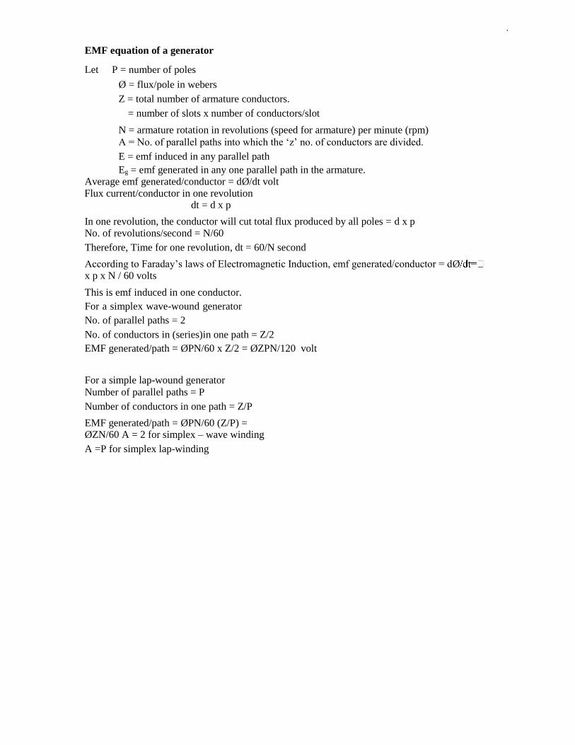
EMF equation of a generator

Let P = number of poles

Ø = flux/pole in webers Z = total number of armature conductors.

= number of slots x number of conductors/slot

N = armature rotation in revolutions (speed for armature) per minute (rpm) A = No. of parallel paths into which the ‘z’ no. of conductors are divided. E = emf induced in any parallel path Eg = emf generated in any one parallel path in the armature.

Average emf generated/conductor = dØ/dt volt Flux current/conductor in one revolution

dt = d x p In one revolution, the conductor will cut total flux produced by all poles = d x p No. of revolutions/second = N/60 Therefore, Time for one revolution, dt = 60/N second According to Faraday’s laws of Electromagnetic Induction, emf generated/conductor = dØx p x N / 60 volts This is emf induced in one conductor. For a simplex wave-wound generator No. of parallel paths = 2 No. of conductors in (series)in one path = Z/2 EMF generated/path = ØPN/60 x Z/2 = ØZPN/120 volt For a simple lap-wound generator Number of parallel paths = P Number of conductors in one path = Z/P EMF generated/path = ØPN/60 (Z/P) = ØZN/60 A = 2 for simplex – wave winding A =P for simplex lap-winding

Armature Reaction and Commutation

Introduction

In a d.c. generator, the purpose of field winding is to produce magnetic field (called main flux) whereas the purpose of armature winding is to carry armature current. Although the armature winding is not provided for the purpose of producing a magnetic field, nevertheless the current in the armature winding will also produce magnetic flux (called armature flux). The armature flux distorts and weakens the main flux posing problems for the proper operation of the d.c. generator. The action of armature flux on the main flux is called armature reaction. 2.1 Armature Reaction

So far we have assumed that the only flux acting in a d.c. machine is that due to the main poles called main flux. However, current flowing through armature conductors also creates a magnetic flux (called armature flux) that distorts and weakens the flux coming from the poles. This distortion and field weakening takes place in both generators and motors. The action of armature flux on the main flux is known as armature reaction. The phenomenon of armature reaction in a d.c. generator is shown in Fig.(2.1)

Only one pole is shown for clarity. When the generator is on no-load, a small current flowing in the armature does not appreciably affect the main flux f1 coming from the pole [See Fig 2.1 (i)]. When the generator is loaded, the current flowing through armature conductors sets up flux f1. Fig. (2.1) (ii) shows flux due to armature current alone. By superimposing f1 and f2, we obtain the resulting flux f3 as shown in Fig. (2.1) (iii). Referring to Fig (2.1) (iii), it is clear that flux density at; the trailing pole tip (point B) is increased while at the leading pole tip (point 4. it is decreased. This unequal field distribution produces the following two effects:

The main flux is distorted. Due to higher flux density at pole tip B, saturation sets in. Consequently, the increase in flux

at pole tip B is less than the decrease in flux under pole tip A. Flux f3 at full load is, therefore, less than flux f1 at no load. As we shall see, the weakening of flux due to armature reaction depends upon the position of brushes.

Fig. (2.1) 2.2 Geometrical and Magnetic Neutral Axes 4. The geometrical neutral axis (G.N.A.) is the axis that bisects the angle between the centre line of

Fig. (2.2)

4. The magnetic neutral axis (M. N. A.) is the axis drawn perpendicular to the mean direction of the flux passing through the centre of the armature. Clearly, no e.m.f. is produced in the armature conductors along this axis because then they cut no flux. With no current in the armature conductors, the M.N.A. coincides with G, N. A. as shown in Fig. (2.2).

5. In order to achieve sparkless commutation, the brushes must lie along M.N.A. 2.3 Explanation of Armature Reaction

With no current in armature conductors, the M.N.A. coincides with G.N.A. However, when current flows in armature conductors, the combined action of main flux and armature flux shifts the M.N.A. from G.N.A. In case of a generator, the M.N.A. is shifted in the direction of rotation of the machine. Inorder to achieve sparkless commutation, the brushes have to be moved along the new M.N.A. Under such a condition, the armature reaction produces the following two effects: 1. It demagnetizes or weakens the main flux. 2. It cross-magnetizes or distorts the main flux. Let us discuss these effects of armature reaction by considering a 2-pole generator (though the following remarks also hold good for a multipolar generator).

(i) Fig. (2.3) (i) shows the flux due to main poles (main flux) when the armature conductors carry no current. The flux across the air gap is uniform. The m.m.f. producing the main flux is represented in magnitude and direction by the vector OFm in Fig. (2.3) (i). Note that OFm is perpendicular to G.N.A.

(ii) Fig. (2.3) (ii) shows the flux due to current flowing in armature conductors alone (main poles unexcited). The armature conductors to the left of G.N.A. carry current “in” (´) and those to the right carry current “out” (•). The direction of magnetic lines of force can be found by cork screw rule. It is clear that armature flux is directed downward parallel to the brush axis. The m.m.f. producing the armature flux is represented in magnitude and direction by the vector OFA in Fig. (2.3) (ii).

(iii) Fig. (2.3) (iii) shows the flux due to the main poles and that due to current in armature conductors acting together. The resultant m.m.f. OF is the vector sum of OFm and OFA as shown in Fig. (2.3) (iii). Since M.N.A. is always perpendicular to the resultant m.m.f., the M.N.A. is shifted through an angle q. Note that M.N.A. is shifted in the direction of rotation of the generator.

(iv) In order to achieve sparkless commutation, the brushes must lie along the M.N.A. Consequently, the brushes are shifted through an angle q so as to lie along the new M.N.A. as shown in Fig. (2.3) (iv). Due to brush shift, the m.m.f. FA of the armature is also rotated through the same angle q. It is because some of the conductors which were earlier under N-pole now come under S-pole and vice-versa. The result is that armature m.m.f. FA will no longer be vertically downward but will be rotated in the direction of rotation through an angle q as shown in Fig. (2.3) (iv). Now FA can be resolved into

Fig. (2.3)

(a) The component Fd is in direct opposition to the m.m.f. OFm due to main poles. It has a demagnetizing effect on the flux due to main poles. For this reason, it is called the demagnetizing or weakening component of armature reaction.

(b) The component Fc is at right angles to the m.m.f. OFm due to main poles. It distorts the main field. For this reason, it is called the cross magnetizing or distorting component of armature reaction. It may be noted that with the increase of armature current, both demagnetizing and distorting effects will increase.

Conclusions (i) With brushes located along G.N.A. (i.e., q = 0°), there is no demagnetizing component of

armature reaction (Fd = 0). There is only distorting or cross magnetizing effect of armature reaction.

(ii) With the brushes shifted from G.N.A., armature reaction will have both demagnetizing and distorting effects. Their relative magnitudes depend on the amount of shift. This shift is directly proportional to the Armature current.

(iii) The demagnetizing component of armature reaction weakens the main flux. On the other hand, the distorting component of armature reaction distorts the main flux.

(iv) The demagnetizing effect leads to reduced generated voltage while cross magnetizing effect leads to sparking at the brushes.

2.4 Demagnetizing and Cross-Magnetizing Conductors

With the brushes in the G.N.A. position, there is only cross-magnetizing effect of armature reaction. However, when the brushes are shifted from the G.N.A. position, the armature reaction will have both demagnetizing and cross magnetizing effects. Consider a 2-pole generator with brushes shifted (lead) θm mechanical degrees from G.N.A. We shall identify the armature conductors that produce demagnetizing effect and those that produce cross-magnetizing effect.

(i) The armature conductors θm on either side of G.N.A. produce flux in direct opposition to main flux as shown in Fig. (2.4) (i). Thus the conductors lying within angles AOC = BOD = 2 θm at the top and bottom of the armature produce demagnetizing effect. These are called demagnetizing armature conductors and constitute the demagnetizing ampere-turns of armature reaction (Remember two conductors constitute a turn).

Fig.(2.4) (ii) The axis of magnetization of the remaining armature conductors lying between angles AOD

and COB is at right angles to the main flux as shown in Fig. (2.4) (ii). These conductors produce the cross-magnetizing (or distorting) effect i.e., they produce uneven flux distribution on each pole. Therefore, they are called cross-magnetizing conductors and constitute the cross-magnetizing ampere-turns of armature reaction. 2.5 Calculation of Demagnetizing Ampere-Turns Per Pole (ATd/Pole)

It is sometimes desirable to neutralize the demagnetizing ampere-turns of armature reaction. This is achieved by adding extra ampere-turns to the main field winding. We shall now calculate the demagnetizing ampere-turns per pole (ATd/pole).

Let Z = total number of armature conductors

I = current in each armature conductor

= Ia/2 ... for simplex wave winding

= Ia/P ... for simplex lap winding

θm = forward lead in mechanical degrees

Note. When a conductor passes a pair of poles, one cycle of voltage is generated. We say one cycle contains 360 electrical degrees. Suppose there are P poles in a generator. In one revolution, there are 360 mechanical degrees and 360 *P/2 electrical degrees. 2.6 Cross-Magnetizing Ampere-Turns Per Pole (ATc/Pole) We now calculate the cross-magnetizing ampere-turns per pole (ATc/pole). (found as above) Cross-magnetizing ampere-turns/pole are

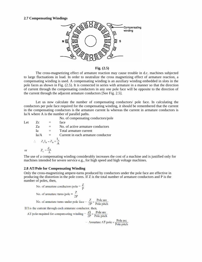
2.7 Compensating Windings

Fig. (2.5)

The cross-magnetizing effect of armature reaction may cause trouble in d.c. machines subjected to large fluctuations in load. In order to neutralize the cross magnetizing effect of armature reaction, a compensating winding is used. A compensating winding is an auxiliary winding embedded in slots in the pole faces as shown in Fig. (2.5). It is connected in series with armature in a manner so that the direction of current through the compensating conductors in any one pole face will be opposite to the direction of the current through the adjacent armature conductors [See Fig. 2.5].

Let us now calculate the number of compensating conductors/ pole face. In calculating the conductors per pole face required for the compensating winding, it should be remembered that the current in the compensating conductors is the armature current Ia whereas the current in armature conductors is Ia/A where A is the number of parallel paths.

Let Zc = No. of compensating conductors/pole face

Za = No. of active armature conductors Ia = Total armature current Ia/A = Current in each armature conductor The use of a compensating winding considerably increases the cost of a machine and is justified only for machines intended for severe service e.g., for high speed and high voltage machines. 2.8 AT/Pole for Compensating Winding Only the cross-magnetizing ampere-turns produced by conductors under the pole face are effective in producing the distortion in the pole cores. If Z is the total number of armature conductors and P is the number of poles, then,

2.9 Commutation

Fig. (2.6) shows the schematic diagram of 2-pole lap-wound generator. There are two parallel paths between the brushes. Therefore, each coil of the winding carries one half (Ia/2 in this case) of the total current (Ia) entering or leaving the armature.

Note that the currents in the coils connected to a brush are either all towards the brush (positive brush) or all directed away from the brush (negative brush). Therefore, current in a coil will reverse as the coil passes a brush. This reversal of current as the coil passes & brush is called commutation.

Fig. (2.6)

The reversal of current in a coil as the coil passes the brush axis is called commutation. When commutation takes place, the coil undergoing commutation is short circuited by the brush. The brief period during which the coil remains short circuited is known as commutation period Tc. If the current reversal is completed by the end of commutation period, it is called ideal commutation. If the current reversal is not completed by that time, then sparking occurs between the brush and the commutator which results in progressive damage to both. Ideal commutation

Let us discuss the phenomenon of ideal commutation (i.e., coil has no inductance) in one coil in the armature winding shown in Fig. (2.6) above. For this purpose, we consider the coil A. The brush width is equal to the width of one commutator segment and one mica insulation. Suppose the total armature current is 40 A. Since there are two parallel paths, each coil carries a current of 20 A.

(i) In Fig. (2.7) (i), the brush is in contact with segment 1 of the commutator. The commutator segment 1 conducts a current of 40 A to the brush; 20 A from coil A and 20 A from the adjacent coil as shown. The coil A has yet to undergo commutation.

(ii) As the armature rotates, the brush will make contact with segment 2 and thus short-circuits the coil A as shown in Fig. (2.7) (ii). There are now two parallel paths into the brush as long as the short-circuit of coil A exists. Fig. (2.7) (ii) shows the instant when the brush is one-fourth on segment 2 and three-fourth on segment 1. For this condition, the resistance of the path through segment 2 is three times the resistance of the path through segment 1 (Q contact resistance varies inversely as the area of contact of brush with the segment). The brush again conducts a current of 40 A; 30 A through segment 1 and 10 A through segment 2. Note that current in coil A (the coil undergoing commutation) is reduced from 20 A to 10 A.

(iii) Fig. (2.7) (iii) shows the instant when the brush is one-half on segment 2 and one-half on segment 1. The brush again conducts 40 A; 20 A through segment 1 and 20 A through segment 2 (Q now the resistances of the two parallel paths are equal). Note that now. current in coil A is zero.

(iv) Fig. (2.7) (iv) shows the instant when the brush is three-fourth on segment 2 and one-fourth on segment 1. The brush conducts a current of 40 A; 30 A through segment 2 and 10 A through segment 1. Note that current in coil A is 10 A but in the reverse direction to that before the start of commutation. The reader may see the action of the commutator in

(v) Fig. (2.7) (v) shows the instant when the brush is in contact only with segment 2. The brush

again conducts 40 A; 20 A from coil A and 20 A from the adjacent coil to coil A. Note that now current in coil A is 20 A but in the reverse direction. Thus the coil A has undergone commutation. Each coil undergoes commutation in this way as it passes the brush axis. Note that during commutation, the coil under consideration remains short circuited by the brush. Fig. (2.8) shows the current-time graph for the coil A undergoing commutation. The horizontal line AB represents a constant current of 20 A upto the beginning of commutation. From the finish of commutation, it is represented by another horizontal line CD on the opposite side of the zero line and the same distance from it as AB i.e., the current has exactly reversed (- 20 A). The way in which current changes from B to C depends upon the conditions under which the coil undergoes commutation. If the current changes at a uniform rate (i.e., BC is a straight line), then it is called ideal commutation as shown in Fig. (2.8). Under such conditions, no sparking will take place between the brush and the commutator.

Fig. (2.7)

Fig. (2.8)

Practical difficulties The ideal commutation (i.e., straight line change of current) cannot be attained in practice. This is

mainly due to the fact that the armature coils have appreciable inductance. When the current in the coil undergoing commutation changes, self-induced e.m.f. is produced in the coil. This is generally called reactance voltage. This reactance voltage opposes the change of current in the coil undergoing commutation. The result is that the change of current in the coil undergoing commutation occurs more slowly than it would be under ideal commutation. This is illustrated in Fig. (2.9). The straight line RC represents the ideal commutation whereas the curve BE represents the change in current when self-inductance of the coil is taken into account. Note that current CE (= 8A in Fig. 2.9) is flowing from the commutator segment 1 to the brush at the instant when they part company. This results in sparking just as when any other current carrying circuit is broken. The sparking results in overheating of commutators brush contact and causing damage to both. Fig. (2.10) illustrates how sparking takes place between the commutators segment and the brush. At the end of commutation or short-circuit period, the current in coil A is reversed to a value of 12 A (instead of 20 A) due to inductance of the coil. When the brush breaks contact with segment 1, the remaining 8 A current jumps from segment 1 to the brush through air causing sparking between segment 1 and the brush.

Fig. (2.9) Fig. (2.10)

2.10 Calculation of Reactance Voltage Reactance voltage = Coefficient of self-inductance *Rate of change of current When a coil undergoes commutation, two commutator segments remain short circuited by the brush. Therefore, the time of short circuit (or commutation period Tc) is equal to the time required by the commutator to move a distance equal to the circumferential thickness of the brush minus the thickness of one insulating strip of mica

Let Wb = brush width in cm;

Wm = mica thickness in cm

v = peripheral speed of commutator in cm/s The commutation period is very small, say of the order of 1/500 second. Let the current in the coil undergoing commutation change from + I to – I (amperes) during the commutation. If L is the inductance of the coil, then reactance voltage is given by; Reactance voltage, ER = L*2I/Tc 2.11 Methods of Improving Commutation Improving commutation means to make current reversal in the short-circuited coil as sparkless as possible. The following are the two principal methods of improving commutation: (i) Resistance commutation (ii) E.M.F. commutation 2.12 Resistance Commutation

The reversal of current in a coil (i.e., commutation) takes place while the coil is short-circuited by the brush. Therefore, there are two parallel paths for the current as long as the short circuit exists. If the contact resistance between the brush and the commutator is made large, then current would divide in the inverse ratio of contact resistances (as for any two resistances in parallel). This is the key point in improving commutation. This is achieved by using carbon brushes (instead of Cu brushes) which have high contact resistance. This method of improving commutation is called resistance commutation. Figs. (2.11) and (2.12) illustrates how high contact resistance of carbon brush improves commutation (i.e., reversal of current) in coil A.

In Fig. (2.11) (i), the brush is entirely on segment 1 and, therefore, the current in coil A is 20 A. The coil A is yet to undergo commutation. As the armature rotates, the brush short circuits the coil A and there are two parallel paths for the current into the brush. Fig. (2.11) (ii) shows the instant when the brush is one-fourth on segment 2 and three-fourth on segment 1. The equivalent electric circuit is shown in Fig. (2.11) (iii) where R1 and R2 represent the brush contact resistances on segments 1 and 2. A resistor is not shown for coil A since it is assumed that the coil resistance is negligible as compared to the brush contact resistance

.

The values of current in the parallel paths of the equivalent circuit are determined by the

respective resistances of the paths. For the condition shown in Fig. (2.11) (ii), resistor R2 has three times the resistance of resistor R1. Therefore, the current distribution in the paths will be as shown. Note that current in coil A is reduced from 20 A to10 A due to division of current in (he inverse ratio of contact resistances. If the Cu brush is used (which has low contact resistance), R1 R2 and the current in coil A would not have reduced to 10 A.

As the carbon brush passes over the commutator, the contact area with segment 2 increases and that with segment 1 decreases i.e., R2 decreases and R1 increases. Therefore, more and more current passes to the brush through segment 2. This is illustrated in Figs. (2.12) (i) and (2.12) (ii), When the break between the brush and the segment 1 finally occurs [See Fig. 2.12 (iii)], the current in the coil is reversed and commutation is achieved. It may be noted that the main cause of sparking during commutation is the production of reactance voltage and carbon brushes cannot prevent it. Nevertheless, the carbon brushes do help in improving commutation. The other minor advantages of carbon brushes are: (i) The carbon lubricates and polishes the commutator. (ii) If sparking occurs, it damages the commutator less than with copper brushes and the damage to the

brush itself is of little importance. 2.13 E.M.F. Commutation

In this method, an arrangement is made to neutralize the reactance voltage by producing a reversing voltage in the coil undergoing commutation. The reversing voltage acts in opposition to the reactance voltage and neutralizes it to some extent. If the reversing voltage is equal to the reactance voltage, the effect of the latter is completely wiped out and we get sparkless commutation. The reversing voltage may be produced in the following two ways: (i) By brush shifting (ii) By using interpoles or compoles (i) By brush shifting In this method, the brushes are given sufficient forward lead (for a generator) to bring the short-circuited coil (i.e., coil undergoing commutation) under the influence of the next pole of opposite polarity. Since the short-circuited coil is now in the reversing field, the reversing voltage produced cancels the reactance voltage. This method suffers from the following drawbacks:

(a) The reactance voltage depends upon armature current. Therefore, the brush shift will depend on the magnitude of armature current which keeps on changing. This necessitates frequent shifting of brushes.

(b) The greater the armature current, the greater must be the forward lead for a generator. This increases the demagnetizing effect of armature reaction and further weakens the main field.

(ii) By using interpoles or compotes The best method of neutralizing reactance voltage is by, using interpoles or compoles.

2.14 Interpoles or Compoles

The best way to produce reversing voltage to neutralize the reactance voltage is by using interpoles or compoles. These are small poles fixed to the yoke and spaced mid-way between the main poles (See Fig. 2.13). They are wound with comparatively few turns and connected in series with the armature so that they carry armature current. Their polarity is the same as the next main pole ahead in the direction of rotation for a generator (See Fig. 2.13). Connections for a d.c. generator with interpoles is shown in Fig. (2.14).

Fig. (2.13) Fig. (2.14) Functions of Interpoles The machines fitted with interpoles have their brushes set on geometrical neutral axis (no lead). The interpoles perform the following two functions: (i) As their polarity is the same as the main pole ahead (for a generator), they induce an e.m.f. in the coil (undergoing commutation) which opposes reactance voltage. This leads to sparkless commutation. The e.m.f. induced by compoles is known as commutating or reversing e.m.f. Since the interpoles carry the armature current and the reactance voltage is also proportional to armature current, the neutralization of reactance voltage is automatic.

Fig. (2.15)

(ii) The m.m.f. of the compoles neutralizes the cross-magnetizing effect of armature reaction in small region in the space between the main poles. It is because the two m.m.f.s oppose each other in this region. Fig. (2.15) shows the circuit diagram of a shunt generator with commutating winding and compensating winding. Both these windings are connected in series with the armature and so they carry the armature current. However, the functions they perform must be understood clearly. The main function of commutating winding is to produce reversing (or commutating) e.m.f. in order to cancel the reactance voltage. In addition to this, the m.m.f. of the commutating winding neutralizes the cross magnetizing ampere-turns in the space between the main poles. The compensating winding neutralizes the cross-magnetizing effect of armature reaction under the pole faces.

UNIT III

TYPES OF DC GENERATORS

Permanent Magnet DC G

When the flux in the magnetic circuit is established by the help of permanent magnets then it is known as Permanent magnet dc generator. It consists of an armature and one or several permanent magnets situated around the armature. This type of dc generators generates very low power. So, they are rarely found in industrial applications. They are normally used in small applications like dynamos in motor cycles.

Separately Excited DC Generator These are the generators whose field magnets are energized by some external dc source such as battery . A circuit diagram of separately excited DC generator is shown in figure.

Ia = Armature current IL = Load current V = Terminal voltage Eg = Generated emf

Voltage drop in the armature = Ia × Ra (R/sub>a is the armature resistance) Let, Ia = IL = I (say) Then,

voltage across the load, V = IRa Power generated, Pg = Eg×I Power delivered to the external load, PL =

V×I.

Self-excited DC Generators These are the generators whose field magnets are energized by the current supplied by themselves. In these type of machines field coils are internally connected with the armature. Due to residual magnetism some flux is always present in the poles. When the armature is rotated some emf is induced. Hence some induced current is produced. This small current flows through the field coil as well as the load and

UNIT-IIID.CGENERATORS – IIUNIT-III

D.C GENERATORS-II UNIT-III

thereby strengthening the pole flux. As the pole flux strengthened, it will produce more armature emf, which cause further increase of current through the field. This increased field current further raises armature emf and this cumulative phenomenon continues until the excitation reaches to the rated value. According to the position of the field coils the Self-excited DC generators may be classified as…

A. Series wound generators B. Shunt wound generators C. Compound wound generators

Series Wound Generator In these type of generators, the field windings are connected in series with armature conductors as shown in figure below. So, whole current flows through the field coils as well as the load. As series field winding carries full load current it is designed with relatively few turns of thick wire. The electrical resistance of series field winding is therefore very low (nearly 0.5Ω ). Let, Rsc = Series winding resistance Isc = Current flowing through the series field Ra = Armature resistance Ia = Armature current IL = Load current V = Terminal voltage Eg = Generated emf

Then, Ia = Isc = IL=I (say) Voltage across the load, V = Eg -I(Ia×Ra) Power generated, Pg = Eg×I Power

delivered to the load, PL = V×I

Shunt Wound DC Generators In these type of DC generators the field windings are connected in parallel with armature conductors as shown in figure below. In shunt wound generators the voltage in the field winding is same as the voltage across the terminal. Let, Rsh = Shunt winding resistance Ish = Current flowing through the shunt field Ra = Armature resistance Ia = Armature current IL = Load current V = Terminal voltage Eg = Generated emf

Here armature current Ia is dividing in two parts, one is shunt field current Ish and another is load current IL. So, Ia=Ish + IL The effective power across the load will be maximum when IL will be maximum. So, it is required to keep shunt field current as small as possible. For this purpose the resistance of the shunt field winding generally kept high (100 Ω) and large no of turns are used for the desired emf. Shunt field current, Ish = V/Rsh Voltage across the load, V = Eg-Ia Ra Power generated, Pg= Eg×Ia Power delivered to the load, PL = V×IL

Compound Wound DC Generator In series wound generators, the output voltage is directly proportional with load current. In shunt wound generators, output voltage is inversely proportional with load current. A combination of these two types of generators can overcome the disadvantages of both. This combination of windings is called compound wound DC generator. Compound wound generators have both series field winding and shunt field winding. One winding is placed in series with the armature and the other is placed in parallel with the armature. This type of DC generators may be of two types- short shunt compound wound generator and long shunt compound wound generator.

Short Shunt Compound Wound DC Generator The generators in which only shunt field winding is in parallel with the armature winding as shown in

figure.

Series field current, Isc = IL Shunt field current, Ish = (V+Isc Rsc)/Rsh Armature current, Ia = Ish + IL Voltage

across the load, V = Eg - Ia Ra - Isc Rsc Power generated, Pg = Eg×Ia Power delivered to the load, PL=V×IL

Long Shunt Compound Wound DC Generator The generators in which shunt field winding is in parallel with both series field and armature winding as

shown in figure. Shunt field current, Ish=V/Rsh Armature current, Ia= series field current, Isc= IL+Ish Voltage across the load, V=Eg-Ia Ra-Isc Rsc=Eg-Ia (Ra+Rsc) [∴Ia=Ics] Power generated, Pg= Eg×Ia Power delivered to the load, PL=V×IL In a compound wound generator, the shunt field is stronger than the series field. When the series field assists the shunt field, generator is said to be commutatively compound wound. On the other hand if series field

opposes the shunt field, the generator is said to be differentially compound wound.

D.C. GENERATOR CHARACTERISTICS

Introduction The speed of a d.c. machine operated as a generator is fixed by the prime mover. For general-purpose operation, the prime mover is equipped with a speed governor so that the speed of the generator is practically constant. Under such condition, the generator performance deals primarily with the relation between excitation, terminal voltage and load. These relations can be best exhibited graphically by means of curves known as generator characteristics. These characteristics show at a glance the behaviour of the generator under different load conditions. 3.1 D.C. Generator Characteristics The following are the three most important characteristics of a d.c. generator: Open Circuit Characteristic (O.C.C.) This curve shows the relation between the generated e.m.f. at no-load (E0) and the field current (If) at constant speed. It is also known as magnetic characteristic or no-load saturation curve. Its shape is practically the same for all generators whether separately or self-excited. The data for O.C.C. curve are obtained experimentally by operating the generator at no load and constant speed and recording the change in terminal voltage as the field current is varied. External characteristic (V/IL) This curve shows the relation between the terminal voltage (V) and load current (IL). The terminal voltage V will be less than E due to voltage drop in the armature circuit. Therefore, this curve will lie below the internal characteristic. This characteristic is very important in determining the suitability of a generator for a given purpose. It can be obtained by making simultaneous measurements of terminal voltage and load current (with voltmeter and ammeter) of a loaded generator.

Internal or Total characteristic (E/Ia) This curve shows the relation between the generated e.m.f. on load (E) and the armature current (Ia). The e.m.f. E is less than E0 due to the demagnetizing effect of armature reaction. Therefore, this curve will lie below the open circuit characteristic (O.C.C.). The internal characteristic is of interest chiefly to the designer. It cannot be obtained directly by experiment. It is because a voltmeter cannot read the e.m.f. generated on load due to the voltage drop in armature resistance. The internal characteristic can be obtained from external characteristic if winding resistances are known because armature reaction effect is included in both characteristics.

3.2 Open Circuit Characteristic of a D.C. Generator The O.C.C. for a d.c. generator is determined as follows. The field winding of the d.c. generator (series or shunt) is disconnected from the machine and is separately excited from an external d.c. source as shown in Fig. (3.1) (ii). The generator is run at fixed speed (i.e., normal speed). The field current (If) is increased from zero in steps and the corresponding values of generated e.m.f. (E0) read off on a voltmeter connected across the armature terminals. On plotting the relation between E0 and If, we get the open circuit characteristic as shown in Fig. (3.1) (i). Fig. (3.1) The following points may be noted from O.C.C.: 4. When the field current is zero, there is some generated e.m.f. OA. This is due to the residual magnetism in the field poles. 5. Over a fairly wide range of field current (upto point B in the curve), the curve is linear. It is because in this range, reluctance of iron is negligible as compared with that of air gap. The air gap reluctance is constant and hence linear relationship. 6. After point B on the curve, the reluctance of iron also comes into picture. It is because at higher flux densitie r for iron decreases and reluctance

of iron is no longer negligible. Consequently, the curve deviates from linear relationship. (iv) After point C on the curve, the magnetic saturation of poles begins and E0 tends to level off. The reader may note that the O.C.C. of even self-excited generator is obtained by running it as a separately excited generator.

3.3 Characteristics of a Separately Excited D.C. Generator The obvious disadvantage of a separately excited d.c. generator is that we require an external d.c. source for excitation. But since the output voltage may be controlled more easily and over a wide range (from zero to a maximum), this type of excitation finds many applications. (i) Open circuit characteristic.

The O.C.C. of a separately excited generator is determined in a manner described in Sec. (3.2). Fig. (3.2) shows the variation of generated e.m f. on no load with field current for various fixed speeds. Note that if the value of constant speed is increased, the steepness of the curve also increases. When the field current is zero, the residual magnetism in the poles will give rise to the small initial e.m.f. as shown. Fig. (3.2)

(ii) Internal and External Characteristics The external characteristic of a separately excited generator is the curve between the terminal voltage (V) and the load current IL (which is the same as armature current in this case). In order to determine the external characteristic, the circuit set up is as shown in Fig. (3.3) (i). As the load current increases, the terminal voltage falls due to two reasons: (a) The armature reaction weakens the main flux so that actual e.m.f. generated E on load is less than that generated (E0) on no load. (b) There is voltage drop across armature resistance (= ILRa = IaRa). Due to these reasons, the external characteristic is a drooping curve [curve 3 in Fig. 3.3 (ii)]. Note that in the absence of armature reaction and armature drop, the generated e.m.f. would have been E0 (curve 1). The internal characteristic can be determined from external characteristic by adding ILRa drop to the external characteristic. It is because armature reaction drop is included in the external characteristic. Curve 2 is the internal

characteristic of the generator and should obviously lie above the external characteristic.

Fig. (3.3) 3.4 Voltage Build-Up in a Self-Excited Generator Let us see how voltage builds up in a self-excited generator. (i) Shunt generator Consider a shunt generator. If the generator is run at a constant speed, some e.m.f. will be generated due to residual magnetism in the main poles. This small e.m.f. circulates a field current which in turn produces additional flux to reinforce the original residual flux (provided field winding connections are correct). This process continues and the generator builds up the normal generated voltage following the O.C.C. shown in Fig. (3.4) (i). The field resistance Rf can be represented by a straight line passing through the origin as shown in Fig. (3.4) (ii). The two curves can be shown on the same diagram as they have the same ordinate [See Fig. 3.4 (iii)]. Since the field circuit is inductive, there is a delay in the increase in current upon closing the field circuit switch The rate at which the current increases depends

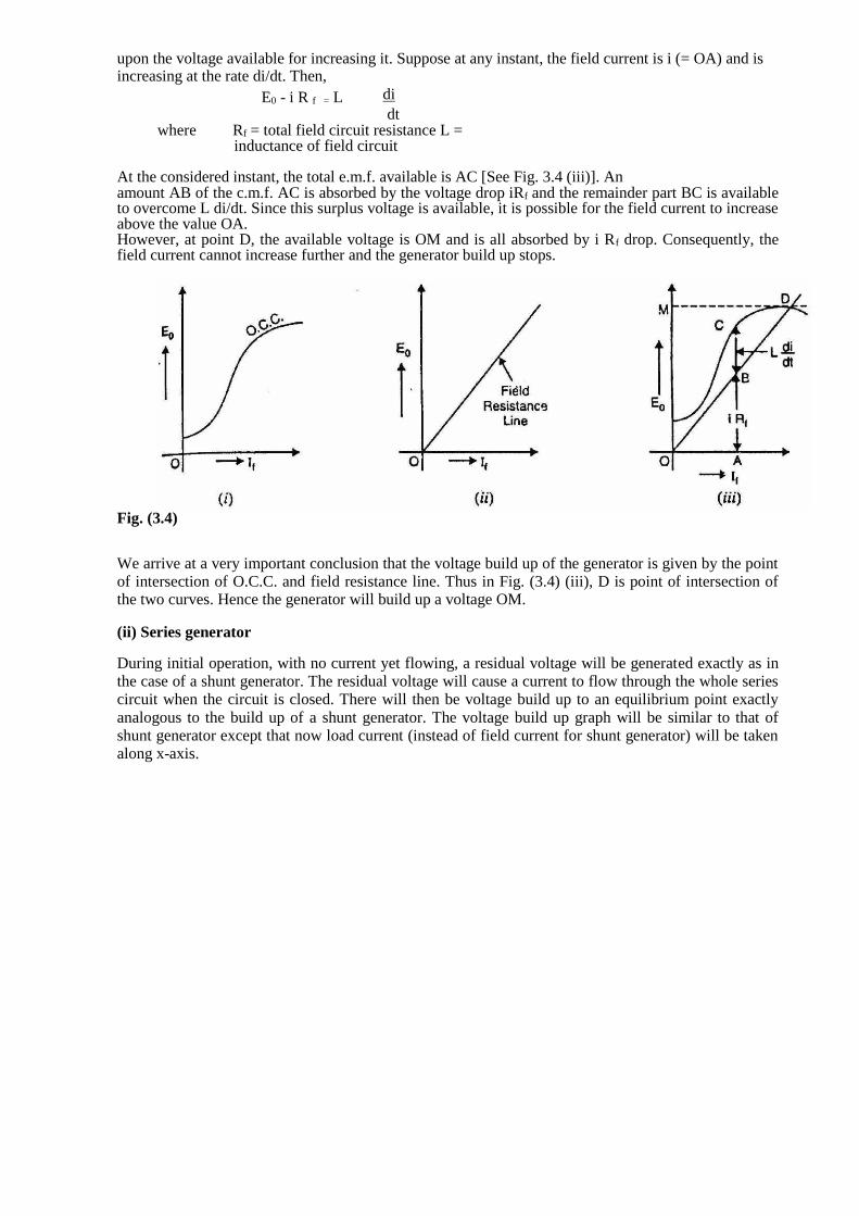
upon the voltage available for increasing it. Suppose at any instant, the field current is i (= OA) and is increasing at the rate di/dt. Then,

E0 - i R f = L di dt

where Rf = total field circuit resistance L = inductance of field circuit

At the considered instant, the total e.m.f. available is AC [See Fig. 3.4 (iii)]. An amount AB of the c.m.f. AC is absorbed by the voltage drop iRf and the remainder part BC is available to overcome L di/dt. Since this surplus voltage is available, it is possible for the field current to increase above the value OA. However, at point D, the available voltage is OM and is all absorbed by i Rf drop. Consequently, the field current cannot increase further and the generator build up stops.

Fig. (3.4)

We arrive at a very important conclusion that the voltage build up of the generator is given by the point of intersection of O.C.C. and field resistance line. Thus in Fig. (3.4) (iii), D is point of intersection of the two curves. Hence the generator will build up a voltage OM. (ii) Series generator During initial operation, with no current yet flowing, a residual voltage will be generated exactly as in the case of a shunt generator. The residual voltage will cause a current to flow through the whole series circuit when the circuit is closed. There will then be voltage build up to an equilibrium point exactly analogous to the build up of a shunt generator. The voltage build up graph will be similar to that of shunt generator except that now load current (instead of field current for shunt generator) will be taken along x-axis.

(iii) Compound generator When a compound generator has its series field flux aiding its shunt field flux, the machine is said to be cumulative compound. When the series field is connected in reverse so that its field flux opposes the shunt field flux, the generator is then differential compound. The easiest way to build up voltage in a compound generator is to start under no load conditions. At no load, only the shunt field is effective. When no-load voltage build up is achieved, the generator is loaded. If under load, the voltage rises, the series field connection is cumulative. If the voltage drops significantly, the connection is differential compound. 3.5 Critical Field Resistance for a Shunt Generator We have seen above that voltage build up in a shunt generator depends upon field circuit resistance. If the field circuit resistance is R1 (line OA), then generator will build up a voltage OM as shown in Fig. (3.5). If the field circuit resistance is increased to R2 (tine OB), the generator will build up a voltage OL, slightly less than OM. As the field circuit resistance is increased, the slope of resistance line also increases. When the field resistance line becomes tangent (line OC) to O.C.C., the generator would just excite. If the field circuit resistance is increased beyond this point (say line OD), the generator will fail to excite. The field circuit resistance represented by line OC (tangent to O.C.C.) is called critical field resistance RC for the shunt generator. It may be defined as under: The maximum field circuit resistance (for a given speed) with which the shunt generator would just excite is known as its critical field resistance. It should be noted that shunt generator will build up voltage only if field circuit resistance is less than critical field resistance. 3.6 Critical Resistance for a Series Generator Fig. (3.6) shows the voltage build up in a series generator. Here R1, R2 etc. represent the total circuit resistance (load resistance and field winding resistance). If the total circuit resistance is R1, then series generator will build up a voltage OL. The Fig. (3.6)

Fig. (3.5)

line OC is tangent to O.C.C. and represents the critical resistance RC for a series generator. If the total resistance of the circuit is more than RC (say line OD), the generator will fail to build up voltage. Note that Fig. (3.6) is similar to Fig. (3.5) with the following differences: (i) In Fig. (3.5), R1, R2 etc. represent the total field circuit resistance. However, R1, R2 etc. in Fig. (3.6) represent the total circuit resistance (load resistance and series field winding resistance etc.). (ii) In Fig (3.5), field current alone is represented along X-axis. However, in Fig. (3.6) load current IL is represented along Y-axis. Note that in a series generator, field current = load current IL.

3.7 Characteristics of Series Generator Fig. (3.7) (i) shows the connections of a series wound generator. Since there is only one current (that which flows through the whole machine), the load current is the same as the exciting current.

Fig. (3.7)

(i) O.C.C. Curve 1 shows the open circuit characteristic (O.C.C.) of a series generator. It can be obtained experimentally by disconnecting the field winding from the machine and exciting it from a separate d.c. source as discussed in Sec. (3.2). (ii) Internal characteristic Curve 2 shows the total or internal characteristic of a series generator. It gives the relation between the generated e.m.f. E. on load and armature current. Due to armature reaction, the flux in the machine will be less than the flux at no load. Hence, e.m.f. E generated under load conditions will be less than the e.m.f. E0 generated under no load conditions. Consequently, internal characteristic curve

lies below the O.C.C. curve; the difference between them representing the effect of armature reaction [See Fig. 3.7 (ii)]. (iii) External characteristic Curve 3 shows the external characteristic of a series generator. It gives the relation between terminal voltage and load current IL:.

a a se Therefore, external characteristic curve will lie below internal characteristic curve by an amount equal to ohmic drop [i.e., Ia(Ra + Rse)] in the machine as shown in Fig. (3.7) (ii).

The internal and external characteristics of a d.c. series generator can be plotted from one another as shown in Fig. (3.8). Suppose we are given the internal characteristic of the generator. Let the line OC represent the resistance of the whole machine i.e. Ra + Rse. If the load current is OB, drop in the machine is AB i.e.

AB = Ohmic drop in the machine = OB(Ra + Rse) Now raise a perpendicular from point B and mark a point b on this line such that ab = AB. Then point b will lie on the external characteristic of the generator. Following similar procedure, other points of external characteristic can be located. It is easy to see that we can also plot internal characteristic from the external characteristic. 3.8 Characteristics of a Shunt Generator Fig (3.9) (i) shows the connections of a shunt wound generator. The armature current Ia splits up into two parts; a small fraction Ish flowing through shunt field winding while the major part IL goes to the external load. (i) O.C.C. The O.C.C. of a shunt generator is similar in shape to that of a series generator as shown in Fig. (3.9) (ii). The line OA represents the shunt field circuit resistance. When the generator is run at normal speed, it will build up a voltage OM. At no-load, the terminal voltage of the generator will be constant (= OM) represented by the horizontal dotted line MC.

Fig. (3.8)

Fig. (3.9) (ii) Internal characteristic When the generator is loaded, flux per pole is reduced due to armature reaction. Therefore, e.m.f. E generated on load is less than the e.m.f. generated at no load. As a result, the internal characteristic (E/Ia) drops down slightly as shown in Fig. (3.9) (ii). (iii) External characteristic Curve 2 shows the external characteristic of a shunt generator. It gives the relation between terminal voltage V and load current IL.

a R a L sh R a Therefore, external characteristic curve will lie below the internal characteristic curve by an amount equal to drop in the armature circuit [i.e., (IL + Ish)Ra] as shown in Fig. (3.9) (ii). Note. It may be seen from the external characteristic that change in terminal voltage from no-load to full load is small. The terminal voltage can always be maintained constant by adjusting the field rheostat R automatically 3.9 Critical External Resistance for Shunt Generator If the load resistance across the terminals of a

shunt generator is decreased, then load current

increase? However, there is a limit to the

increase in load current with the decrease of

load resistance. Any decreaseof load

resistance beyond this point, instead of

increasing the current, ultimatelyresults in Fig. (3.10)

reduced current. Consequently, the external characteristic turns back (dotted curve) as shown in Fig. (3.10). The tangent OA to the curve represents the minimum external resistance required to excite the shunt generator on load and is called critical external resistance. If the resistance of the external circuit is less than the critical external resistance (represented by tangent OA in Fig. 3.10), the machine will refuse to excite or will de-excite if already running This means that external resistance is so low as virtually to short circuit the machine and so doing away with its excitation. Note. There are two critical resistances for a shunt generator viz., (i) critical field resistance (ii) critical external resistance. For the shunt generator to build up voltage, the former should not be exceeded and the latter must not be gone below.

3.10 How to Draw O.C.C. at Different Speeds? If we are given O.C.C. of a generator at a constant speed N1, then we can easily draw the O.C.C. at any other constant speed N2. Fig (3.11) illustrates the procedure. Here we are given O.C.C. at a constant speed N1. It is desired to find the O.C.C. at constant speed N2 (it is assumed that n1 < N2). For constant exci

This locates the point D on the new O.C.C. at N2. Similarly, other points can be located taking different values of If. The locus of these points will be the O.C.C. at N2. 3.11 Critical Speed (NC) The critical speed of a shunt generator is the minimum speed below which it fails to excite. Clearly, it is the speed for which the given shunt field resistance represents the critical resistance. In Fig. (3.12), curve 2 corresponds to critical speed because the shunt field resistance (Rsh) line is tangential to it. If the

generator runs at full speed N, the new O.C.C. moves upward and the R'sh line represents critical resistance for this speed.

In order to find critical speed, take any convenient point C on excitation axis and erect a perpendicular so as to cut Rsh and R'sh lines at points B and A respectively. Then,

N

C

Fig. (3.12)

AC N

N

or C

AC

3.12 Conditions for Voltage Build-Up of a Shunt Generator The necessary conditions for voltage build-up in a shunt generator are: (v) There must be some residual magnetism in generator poles. (vi) The connections of the field winding should be such that the field current strengthens the

residual magnetism. (vii) The resistance of the field circuit should be less than the critical resistance. In other words, the

speed of the generator should be higher than the critical speed. 3.13 Compound Generator Characteristics In a compound generator, both series and shunt excitation are combined as shown in Fig. (3.13). The shunt winding can be connected either across the armature only (short-shunt connection S) or across armature plus series field (long-shunt connection G). The compound generator can be cumulatively compounded or differentially compounded generator. The latter is rarely used in practice. Therefore, we shall discuss the characteristics of cumulatively-compounded generator. It may be noted that external characteristics of long and short shunt compound generators are almost identical. External characteristic Fig. (3.14) shows the external characteristics of a cumulatively compounded generator. The series excitation aids the shunt excitation. The degree of

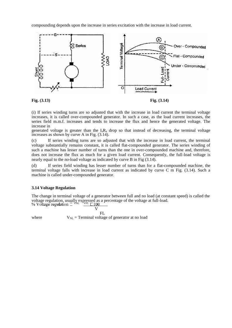
compounding depends upon the increase in series excitation with the increase in load current. Fig. (3.13) Fig. (3.14)

(i) If series winding turns are so adjusted that with the increase in load current the terminal voltage increases, it is called over-compounded generator. In such a case, as the load current increases, the series field m.m.f. increases and tends to increase the flux and hence the generated voltage. The increase in generated voltage is greater than the IaRa drop so that instead of decreasing, the terminal voltage increases as shown by curve A in Fig. (3.14). (c) If series winding turns are so adjusted that with the increase in load current, the terminal voltage substantially remains constant, it is called flat-compounded generator. The series winding of such a machine has lesser number of turns than the one in over-compounded machine and, therefore, does not increase the flux as much for a given load current. Consequently, the full-load voltage is nearly equal to the no-load voltage as indicated by curve B in Fig (3.14). (d) If series field winding has lesser number of turns than for a flat-compounded machine, the terminal voltage falls with increase in load current as indicated by curve C m Fig. (3.14). Such a machine is called under-compounded generator. 3.14 Voltage Regulation The change in terminal voltage of a generator between full and no load (at constant speed) is called the voltage regulation, usually expressed as a percentage of the voltage at full-load.

VNL VFL V

FL where VNL = Terminal voltage of generator at no load

VFL = Terminal voltage of generator at full load

Note that voltage regulation of a generator is determined with field circuit and speed held constant. If the voltage regulation of a generator is 10%, it means that terminal voltage increases 10% as the load is changed from full load to no load. 3.15 Parallel Operation of D.C. Generators In a d.c. power plant, power is usually supplied from several generators of small ratings connected in parallel instead of from one large generator. This is due to the following reasons: (i) Continuity of service If a single large generator is used in the power plant, then in case of its breakdown, the whole plant will be shut down. However, if power is supplied from a number of small units operating in parallel, then in case of failure of one unit, the continuity of supply can be maintained by other healthy units. (ii) Efficiency Generators run most efficiently when loaded to their rated capacity. Electric power costs less per kWh when the generator producing it is efficiently loaded. Therefore, when load demand on power plant decreases, one or more generators can be shut down and the remaining units can be efficiently loaded. (iii) Maintenance and repair Generators generally require routine-maintenance and repair. Therefore, if generators are operated in parallel, the routine or emergency operations can be performed by isolating the affected generator while load is being supplied by other units. This leads to both safety and economy. (iv) Increasing plant capacity In the modern world of increasing population, the use of electricity is continuously increasing. When added capacity is required, the new unit can be simply paralleled with the old units. (v) Non-availability of single large unit In many situations, a single unit of desired large capacity may not be available. In that case a number of smaller units can be operated in parallel to meet the load requirement. Generally a single large unit is more expensive.

3.16 Connecting Shunt Generators in Parallel The generators in a power plant are connected in parallel through bus-bars. The bus-bars are heavy

tors are .connected to the +ve side of bus-bars and negative terminals to the negative side of bus-bars. Fig. (3.15) shows shunt generator 1 connected to the bus-bars and supplying load. When the load on the power plant increases beyond the capacity of this generator, the second shunt generator 2 is connected in parallel wish the first to meet the increased load demand. The procedure for paralleling generator 2 with generator 1 is as under: (i) The prime mover of generator 2 is brought up to the rated speed. Now switch S4 in the field circuit of the generator 2 is closed. Fig. (3.15)

(ii) Next circuit breaker CB-2 is closed and the excitation of generator 2 is adjusted till it generates voltage equal to the bus-bars voltage. This is indicated by voltmeter V2. (v) Now the generator 2 is ready to be paralleled with generator 1. The main switch S3, is closed, thus putting generator 2 in parallel with generator 1. Note that generator 2 is not supplying any load because its generated e.m.f. is equal to bus-bars voltage. The generator is said to be “floating” (i.e., not supplying any load) on the bus-bars.

(iv) If generator 2 is to deliver any current, then its generated voltage E should be greater than the bus-bars voltage V. In that case, current supplied by it is I =

a where Ra is the resistance of the armature circuit. By increasing the field current (and hence induced e.m.f. E), the generator 2 can be made to supply proper amount of load. (v) The load may be shifted from one shunt generator to another merely by adjusting the field excitation. Thus if generator 1 is to be shut down, the whole load can be shifted onto generator 2 provided it has the capacity to supply that load. In that case, reduce the current supplied by generator 1 to zero (This will be indicated by ammeter A1) open C.B.-1 and then open the main switch S1.

3.17 Load Sharing The load sharing between shunt generators in parallel can be easily regulated because of their drooping characteristics. The load may be shifted from one generator to another merely by adjusting the field excitation. Let us discuss the load sharing of two generators which have unequal no-load voltages. Let E1, E2 = no-load voltages of the two generators R1, R2 = their armature resistances V = common terminal voltage (Bus-bars voltage)

Then E1 Vand I E2

1 2 R 2

1 Thus current output of the generators depends upon the values of E1 and E3. These values may be changed by field rheostats. The common terminal voltage (or bus-bars voltage) will depend upon (i) the e.m.f.s of individual generators and (ii) the total load current supplied. It is generally desired to keep the bus-bars voltage constant. This can be achieved by adjusting the field excitations of the generators operating in parallel.

3.18 Compound Generators in Parallel Under-compounded generators also operate satisfactorily in parallel but over-compounded generators will not operate satisfactorily unless their series fields are paralleled. This is achieved by connecting two negative brushes together as shown in Fig. (3.16) (i). The conductor used to connect these brushes is generally called equalizer bar. Suppose that an attempt is made to operate the two generators in Fig. (3.16) (ii) in parallel without an equalizer bar. If, for any reason, the current supplied by generator 1 increases slightly, the current in its series field will increase and raise the generated voltage. This will cause generator 1 to take more load. Since total load supplied to the system is constant, the current in generator 2 must decrease and as a result its series field is

weakened. Since this effect is cumulative, the generator 1 will take the entire load and drive generator 2 as a motor. Under such conditions, the current in the two machines will be in the direction shown in Fig. (3.16) (ii). After machine 2 changes from a generator to a motor, the current in the shunt field will remain in the same direction, but the current in the armature and series field will reverse. Thus the magnetizing action, of the series field opposes that of the shunt field. As the current taken by the machine 2 increases, the demagnetizing action of series field becomes greater and the resultant field becomes weaker. The resultant field will finally become zero and at that time machine 2 will short-circuit machine 1, opening the breaker of either or both machines.

Fig. (3.16)

When the equalizer bar is used, a stabilizing action exist? and neither machine tends

to take all the load. To consider this, suppose that current delivered by generator 1

increases [See Fig. 3.16 (i)]. The increased current will not only pass through the series

field of generator 1 but also through the equalizer bar and series field of generator 2.

Therefore, the voltage of both the machines increases and the generator 2 will take a part

of the load.

UNIT IV DC MOTOR

A dc motor is similar in construction to a dc generator. As a matter of fact a dc generator will run as a motor when its field & armature windings are connected to a source of direct current. The basic construction is same whether it is generator or a motor. Working principle:

The principle of operation of a dc motor can be stated as when a current carrying conductor is placed in a magnetic field; it experiences a mechanical force. In a practical dc motor, the field winding produces the required magnetic held while armature conductor play the role of current carrying conductor and hence the armature conductors experience a force. As conductors are placed in the slots which are on the periphery, the individual force experienced by the conductive acts as a twisting or turning force on the armature which is called a torque. The torque is the product of force and the radius at which this force acts, so overall armature experiences a torque and starts rotating. Consider a single conductor placed in a magnetic field , the magnetic field is produced by a permanent magnet but in practical dc motor it is produced by the field winding when it carries a current. Now this conductor is excited by a separate supply so that it carries a current in a particular direction. Consider that it carries a current away from an current. Any current carrying conductor produces its own magnetic field around it, hence this conductor also produces its own flux, around. The direction of this flux can be determined by right hand thumb rule. For direction of current considered the direction of flux around a conductor is clock-wise. Now, there are two fluxes present 5. Flux produced by permanent magnet called main flux 6. Flux produced by the current carrying conductor From the figure shown below, it is clear that on one side of the conductor, both the fluxes are in the same direction in this case, on the left of the conductor there gathering of the flux lines as two fluxes help each other. A to against this, on the right of the conductor, the two fluxes are in opposite direction and hence try to cancel each other. Due to this, the density of the flux lines in this area gets weakened. So on the left, there exists high flux density area while on the right of the conductor then exists low flux density area as shown. The flux distribution around the conductor arts like a stretched ribbed bond under tension. The exerts a mechanical force on the conductor which acts from high flux density area towards low flux density area, i.e. from left to right from the case considered as shown above. In the practical dc motor, the permanent magnet is replaced by the field winding which produces the required flux winding which produces the required flux called main flux and all the armature conductors, would on the periphery of the armature gram, get subjected tot he mechanical force. Due to this, overall armature experiences a twisting force called torque and armature of the motor status rotating.

UNIT-IVD.C.MOTORS

UNIT-IVD.C MOTORS

Direction of rotation of motor The magnitude of the force experienced by the conductor in a motor is given by F = BIL newtons. The direction of the main field can be revoked y changing the direction of current passing through the field winding, which is possible by interchanging the polarities of supply which is given to the field winding. The direction of current through armature can be reversed by changing supply polarities of dc supplying current to the armature. It directions of bot the currents are changed then the direction of rotation of the motor remains undamaged. In a dc motor both the field and armature is connected to a source of direct current. The current through the armature winding establish its own magnetic flux the interaction both the main field and the armature current produces the torque, there by sensing the motor to rotate, once the motor starts rotating, already existing magnetic flux there wire be an induced emf in the armature conductors due to generator action. This emf acts in a direction apposite to supplied voltage. Therefore it is called Black emf. Significance of Back emf In the generating action, when a conductor cuts the lines of flux, emf gets induced in the conductor in a motor, after a motoring action, armature starts rotating and armature conductors cut the main flux. After a motoring action, there exists a generating action there is induced emf in the rotating armature conductors according to Faraday’s law of electromagnetic induction. This induced emf in the armature always acts in

the opposite direction of the supply voltage. This is according tot he lenz’s law which states that the direction of the induced emf is always so as to oppose the case producing it. In a dc motor, electrical input i.e., the supply voltage is the cause and hence this induced emf opposes the supply voltage. The emf tries to set u a current throughout he armature which is in the opposite direction to that which supply voltage is forcing through the conductor so, as this emf always opposes the supply voltage, it is called back emf and devoted as Eb. Through it is denoted as Eb, basically it gets generated by the generating action which we have seen

ZNP earlier So, Eb

60 A Voltage equation of a Motor The voltage v applied across the motor armature has to (1) over core the back emf Eb and 3. supply the armature ohmic drop Ia Ra

v = Eb + Ia Ra This is known as voltage equation of a motor Multiplying both sides by Ia, we get Via =Eb Ia + Ea

2 Ra VIa = electrical input to the armature EbIa = electrical equivalent of mechanical Power developed in the armature

Ia

2 Ra = un loss in the armature

Hence, out of the armature input, some in wasted in I2 R loss and the rot is convened into mechanical power within the armature. Motor efficiency is given by the ratio of power developed by the armature to its input i.e. Eb Ia / vIa = Eb/v. Higher the value of Eb as compared to v, higher the motor efficiency. Conduction for maximum powers The gross mechanical developed by a motor = pm = vIa – Ia

2 Ra

dPm a Ra Ia Ra = v/2

dIa

As v = Eb + Ia Ra and Ia Ra = v/2 Eb = v/2 Thus gross mechanical power developed by a motor is maximum when back emf is equal to half the applied voltage. This conduction’s how ever at realized in practice, because in that case current will be

much beyond the normal current of the motor.

More ova, half the input would be wasted in the form of heat and taking other losses into consideration the motor efficiency will be well below 50 %. 1. A 220v – the induced emf when the machine acts (1) generator (2) motor. The dc motor is assumed to be shunt connected in cash case, short current in considered negligible because its value is not given. (a) As generator Eg = v + Ia Ra = 220 + 0.5 x 20 = 230 v (b) As motor Eb = v – Ia Ra = 220 – 0.5 x 20 =210 v

8) the back emf when giving an output at 7.46 kw at 85% efficiency.

Motor input power = 7.46 x103 w 0.85

Motor input current =

7460

0.85x 440 3.

respectively. Determine the total armature power developed when working (1) as generator delivering 25 kw output and (2) as a motor taking 25 kw input.

Voltage equation of dc motor For a generator, generated emf has to supply armature resistance drop and remaining part is available across the loss as a terminal voltage. But in case of dc motor, supply voltage v has to over come back

emf Eb which is opposing v and also various drops are armature resistance drop Ia Ra, brush drop etc. In fact the electrical work done in overcoming the back emf gets converted into the mechanical energy, developed in the armature.

Hence, the voltage equation of a dc motor is V = Eb + Ia Ra + brush drops Or v = Eb + Ia Ra neglecting brush drops

The back emf is always less than supply voltage (Eb < v) but Ra is very small hence under normal running conditions, the different between back emf and supply voltage is very small. The net voltage across the armature is the difference between the supply voltage and back emf which decals the armature current. Hence from the voltage equation we can write Ia = v – Eb / Ra.

3. A 220 v dc motor has an

during a certain load, calculate the induced emf in the motor under this condition.

V = 200 v, Ia = 30A, Ra For a motor , v = Eb + Ia Ra

Eb = 197.5 v This is the induced mef called back emf in a motor. 5. A 4-pole dc motor has lap connected armature winding. The number of armature conductors is

250. When connected to 230 v dc supply it draws an armature current It 4 cm calculate the back emf and the speed with which motor is P = 4 A = P = 4 as lap connected

-3 V = 230v, z = 250 Ia = 40 A

From voltage equation V = Eb + Ia Ra

230 = Eb + 40 x 0.6

206 = (30 x 10-3 x 4 x N x 250) / (60 x 4) N = 1648 rpm.

Torque: The turning or twisting movement of a body is called

Torque. (Or) It is defined as the product of force and perpendicular distance Ť=F*R

F

In case of DC motor torque is produced by the armature and shaft called as armature torque (Ta ) and shaft torque(Tsh). Let, N be the speed of the armature in RPM R be the radius of the armature Power=Work Done/Time Work Done=Force X Distance

The distance travelled in rotating the armature for one time =2∏R If N rotations are made in 60 sec Then time taken for one rotation is=60/N

So, Power= (F * 2∏R)/ (60/N)

= (F*R)(2∏N)/60

P = Ťω

Here P=EbIa But Eb=ØZNP/60A (ØZNP/60A)Ia= Ťω

= Ťa(2∏N)/60 Ťa=0.159ØZ IaP/A Similarly, Shaft torque Tsh=output/ω

Tsh =output/((2∏N)/60) Tsh =9.55(output)/N

UNIT V TESTING OF DC MACHINES

5.1 Introduction

In the previous sections we have learnt about the principle of operation of d.c. generators and motors, (starting and speed control of d.c motor). Motors convert electrical power (input power) into mechanical power (output power) while generators convert mechanical power (input power) into electrical power (output power). Whole of the input power can not be converted into the output power in a practical machine due to various losses that take place within the machine. Efficiency η being the ratio of output power to input power, is always less than 1 (or 100 %). Designer of course will try to make η as large as possible. Order of efficiency of rotating d.c machine is about 80 % to 85 %. It is therefore important to identify the losses which make efficiency poor.

In this lesson we shall first identify the losses and then try to estimate them to get an idea of efficiency of a given d.c machine. 5.2 Major losses Take the case of a loaded d.c motor. There will be copper losses (Ia

2 ra and I 2f R f =VI f ) in armature and field circuit. The armature copper loss is variable and depends upon degree of loading of the machine. For a shunt machine, the field copper loss will be constant if field resistance is not varied. Recall that rotor body is made of iron with slots in which armature conductors are placed. Therefore when armature rotates in presence of field produced by stator field coil, eddy current and hysteresis losses are bound to occur on the rotor body made of iron. The sum of eddy current and hysteresis losses is called the core loss or iron loss. To reduce core loss, circular varnished and slotted laminations or stamping are used to fabricate the armature. The value of the core loss will depend on the strength of the field and the armature speed. Apart from these there will be power loss due to friction occurring at the bearing & shaft and air friction (windage loss) due to rotation of the armature. To summarise following major losses occur in a d.c machine.

UNIT-VTESTING OF DCMACHINES

UNIT-VTESTING OF DC MACHINES

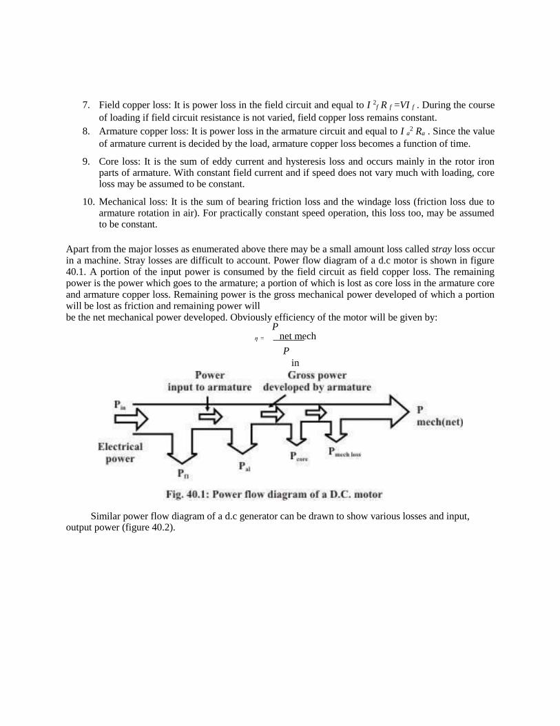
7. Field copper loss: It is power loss in the field circuit and equal to I 2f R f =VI f . During the course

of loading if field circuit resistance is not varied, field copper loss remains constant. 8. Armature copper loss: It is power loss in the armature circuit and equal to I a

2 Ra . Since the value of armature current is decided by the load, armature copper loss becomes a function of time.

9. Core loss: It is the sum of eddy current and hysteresis loss and occurs mainly in the rotor iron

parts of armature. With constant field current and if speed does not vary much with loading, core loss may be assumed to be constant.

10. Mechanical loss: It is the sum of bearing friction loss and the windage loss (friction loss due to

armature rotation in air). For practically constant speed operation, this loss too, may be assumed to be constant.

Apart from the major losses as enumerated above there may be a small amount loss called stray loss occur in a machine. Stray losses are difficult to account. Power flow diagram of a d.c motor is shown in figure 40.1. A portion of the input power is consumed by the field circuit as field copper loss. The remaining power is the power which goes to the armature; a portion of which is lost as core loss in the armature core and armature copper loss. Remaining power is the gross mechanical power developed of which a portion will be lost as friction and remaining power will be the net mechanical power developed. Obviously efficiency of the motor will be given by:

P η = net mech

P in

Similar power flow diagram of a d.c generator can be drawn to show various losses and input, output power (figure 40.2).

It is important to note that the name plate kW (or hp) rating of a d.c machine always corresponds to the net output at rated condition for both generator and motor. 5.3 Swinburne’s Test

For a d.c shunt motor change of speed from no load to full load is quite small. Therefore, mechanical loss can be assumed to remain same from no load to full load. Also if field current is held constant during loading, the core loss too can be assumed to remain same.

In this test, the motor is run at rated speed under no load condition at rated voltage. The current drawn from the supply IL0 and the field current If are recorded (figure 40.3). Now we note that:

Input power to the motor, Pin Cu loss in the field circuit Pfl Power input to the armature,

Cu loss in the armature circuit

Gross power developed by armature

4. VIL0 5. VIf 6. VIL0 - VIf 7. V(IL0 – If) 8. VIa0

= I 2 r a

0 a = VI a

0 −I r

a0 a = (V −I a 0 ra )Ia0

I 7. b 0 a0

Since the motor is operating under no load condition, net mechanical output power is zero. Hence the gross power developed by the armature must supply the core loss and friction & windage losses of the motor. Therefore,

Pcore + Pfriction = ( V − I a 0 ra )I a 0 = Eb 0 Ia0 Since, both Pcore and Pfriction for a shunt motor remains practically constant from no load to full load,

the sum of these losses is called constant rotational loss i.e., constant rotational loss, Prot = Pcore + Pfriction

In the Swinburne's test, the constant rotational loss comprising of core and friction loss is estimated from the above equation.

After knowing the value of Prot from the Swinburne's test, we can fairly estimate the efficiency of the motor at any loading condition. Let the motor be loaded such that new current drawn from the supply is IL and the new armature current is Ia as shown in figure 40.4. To estimate the efficiency of the loaded motor we proceed as follows:

Input power to the motor, Pin = VIL

Cu loss in the field circuit Pfl = VIf Power input to the armature, = VIL - VIf

= V(IL – If) = VIa

Cu loss in the armature circuit = I r a a

Gross power developed by armature = VI a −I a a r

= (V −I a ra )Ia

= Eb Ia

Net mechanical output power, Pnet mech =

E I −P

b a rot

∴ efficiency of the loaded motor, η =

b a rot

VIL

=

net mech

P

in

The estimated value of Prot obtained from Swinburne’s test can also be used to estimate the efficiency of the shunt machine operating as a generator. In figure 40.5 is shown to deliver a load current IL to a load resistor RL. In this case output power being known, it is easier to add the losses to estimate the input mechanical power.

Output power of the generator, Pout Cu loss in the field circuit Pfl Output

power of the armature,

Mechanical input power, Pin mech ∴ Efficiency of the generator, η

9. VIL 10. VIf 11. VIL + VIf 12. VIa + I 2 r + P

13. VI a a a rot

(viii) VIL

in mech

= VIL

VI + I r + P

a a arot

The biggest advantage of Swinburne's test is that the shunt machine is to be run as motor under no

load condition requiring little power to be drawn from the supply; based on the no load reading, efficiency can be predicted for any load current. However, this test is not sufficient if we want to know more about its performance (effect of armature reaction, temperature rise, commutation etc.) when it is actually loaded. Obviously the solution is to load the machine by connecting mechanical load directly on the shaft for motor or by connecting loading rheostat across the terminals for generator operation. This although sounds simple but difficult to implement in the laboratory for high rating machines (say above 20 kW), Thus the laboratory must have proper supply to deliver such a large power corresponding to the rating of the machine. Secondly, one should have loads to absorb this power. 5.4 Hopkinson’s test

This as an elegant method of testing d.c machines. Here it will be shown that while power drawn from the supply only corresponds to no load losses of the machines, the armature physically carries any amount of current (which can be controlled with ease). Such a scenario can be created using two similar mechanically coupled shunt machines. Electrically these two machines are eventually connected in parallel and controlled in such a way that one machine acts as a generator and the other as motor. In other words two similar machines are required to carry out this testing which is not a bad proposition for manufacturer as large numbers of similar machines are manufactured.

Procedure

Connect the two similar (same rating) coupled machines as shown in figure 40.6. With switch S opened, the first machine is run as a shunt motor at rated speed. It may be noted that the second machine is operating as a separately excited generator because its field winding is excited and it is driven by the first machine. Now the question is what will be the reading of the voltmeter connected across the opened switch S? The reading may be (i) either close to twice supply voltage or (ii) small voltage. In fact the voltmeter practically reads the difference of the induced voltages in the armature of the machines. The upper armature terminal of the generator may have either + ve or negative polarity. If it happens to be +ve, then voltmeter reading will be small otherwise it will be almost double the supply voltage.

Since the goal is to connect the two machines in parallel, we must first ensure voltmeter reading is small. In case we find voltmeter reading is high, we should switch off the supply, reverse the armature connection of the generator and start afresh. Now voltmeter is found to read small although time is still not ripe enough to close S for paralleling the machines. Any attempt to close the switch may result into large circulating current as the armature resistances are small. Now by adjusting the field current Ifg of the generator the voltmeter reading may be adjusted to zero (Eg ≈ Eb) and S is now closed. Both the machines are now connected in parallel as shown in figure 40.7.

Loading the machines After the machines are successfully connected in parallel, we go for loading the machines i.e., increasing the armature currents. Just after paralleling the ammeter reading A will be close to zero as Eg ≈ Eb. Now if I fg is increased (by decreasing Rfg), then Eg becomes greater than Eb and both Iag and Iam increase, Thus by increasing field current of generator (alternatively decreasing field current of motor) one can make Eg > Eb so as to make the second machine act as generator and first machine as motor. In practice, it is also required to control the field current of the motor Ifm to maintain speed constant at rated value. The interesting point to be noted here is that Iag and Iam do not reflect in the supply side line. Thus current drawn from supply remains small (corresponding to losses of both the machines). The loading is sustained by the output power of the generator running the motor and vice versa. The machines can be loaded to full load current without the need of any loading arrangement. Calculation of efficiency Let field currents of the machines be are so adjusted that the second machine is acting as generator with armature current Iag and the first machine is acting as motor with armature current Iam as shown in figure 40.7. Also let us assume the current drawn from the supply be I1. Total power drawn from supply is VI1 which goes to supply all the losses (namely Cu losses in armature & field and rotational losses) of both the machines, Now:

Power drawn from supply = VI1

Field Cu loss for motor = VIfm Field Cu loss for generator = VIfg

Armature Cu loss for motor = I r am am

Armature Cu loss for generator = I r ag ag

∴Rotational losses of both the machines = VI1 − ( VI fm + VI fg + I am 2 ram + I ag 2 rag ) (40.1)

Since speed of both the machines are same, it is reasonable to assume the rotational losses of both

the machines are equal; which is strictly not correct as the field current of the generator will be a bit more than the field current of the motor, Thus,

Rotational loss of each machine, P = VI1 − ( VI fm + VI fg + I am 2ram + I ag 2 rag )

rot

2

Once Prot is estimated for each machine we can proceed to calculate the efficiency of the machines as follows, Efficiency of the motor

As pointed out earlier, for efficiency calculation of motor, first calculate the input power and then subtract the losses to get the output mechanical power as shown below,

Total power input to the motor = power input to its field + power input to its armature

Pinm = VI fm +VIam Losses of the motor = VI f

m + I 2 r + P

am am rot

Net mechanical output power Poutm = Pinm − ( VI fm + I am2 ram + Prot )

outm

∴ ηm = P inm

Efficiency of the generator

For generator start with output power of the generator and then add the losses to get the input mechanical power and hence efficiency as shown below,

Output power of the generator, Poutg = VIag

Losses of the generator = VI fg

+ I 2 r + P

P ag ag rot

2

Input power to the generator, Ping = ou

tg + (VI fg + I ag rag + Prot )

outg

∴ ηg

= P ing

5.5 Condition for maximum efficiency

We have seen that in a transformer, maximum efficiency occurs when copper loss = core loss, where, copper loss is the variable loss and is a function of loading while the core loss is practically constant independent of degree of loading. This condition can be stated in a different way: maximum efficiency occurs when the variable loss is equal to the constant loss of the transformer.

Here we shall see that similar condition also exists for obtaining maximum efficiency in a d.c shunt machine as well. Maximum efficiency for motor mode

Let us consider a loaded shunt motor as shown in figure 40.8. The various currents along with their directions are also shown in the figure.

Ia IL +

If

Ia IL

If

+

We assume that field current If remains constant during change of loading. Let,

Prot = constant rotational loss

V If = constant field copper loss Constant loss Pconst = Prot + V If

Now, input power drawn from supply = V IL Power loss in the armature, = I 2 r

a a − I 2 r − (VI

Net mechanical output power = VI + P )

L a a f rot = VI − I 2 r − P L a a const VI − I 2 r − P

so, efficiency at this load current ηm = L a a

const

VIL

Now the armature copper loss Ia

2 ra can be approximated to IL2 ra as Ia ≈ IL . This is because the order

of field current may be 3 to 5% of the rated current. Except for very lightly loaded motor, this assumption is reasonably fair. Therefore replacing Ia by If in the above expression for efficiency ηm , we get,

VI − I 2 r − P

ηm = L L a

const

I VIL

r P

= 1− L a − const V VIL

dηm = 0

dIL

or, d

I r P

= 0

L a

− const

dI

VIL

V

L

ra P

or, − + const

V VIL2

∴Condition for maximum efficiency is I 2 r ≈ I 2 r =

Thus, we get a simplified expression for motor efficiency ηm in terms of the variable current (which

depends on degree of loading) IL, current drawn from the supply. So to find out the condition for maximum efficiency, we have to differentiate ηm with respect to IL and set it to zero as shown below. Maximum efficiency for Generation mode

Similar derivation is given below for finding the condition for maximum efficiency in generator mode by referring to figure 40.9.

We assume that field current If remains constant during change of loading. Let,

Pconst L

a a a

=P r

So, the armature current at which efficiency becomes maximum is Ia

const a

Prot = constant rotational loss

V If = constant field copper loss Constant loss Pconst = Prot + V If

Net output power to load = V IL Power loss in the armature, = I 2 r

a a + I 2 r + (VI

Mechanical input power = VI + P )

L a a f rot = VI + I 2 r + P

L a a const

so, efficiency at this load current ηg =

VIL

VI + I 2 r + P

L a a const

As we did in case of motor, the armature copper loss I 2 r can be approximated to I 2 r as a a L a

Ia ≈ IL . So expression for ηg becomes,

η VIL g = VI + I r + P

L L a const

Thus, we get a simplified expression for motor efficiency ηg in terms of the

variable current (which depends on degree of loading) IL, current delivered to the load. So to find out the condition for maximum efficiency, we have to differentiate ηg with respect to IL and set it to zero as shown below.

Thus maximum efficiency both for motoring and generating are same in case of shunt machines. To state we can say at that armature current maximum efficiency will occur which will make variable loss = constant loss. Eventually this leads to the expression for armature current for maximum efficiency as Ia = Pconst ra .

dηg

= 0

dIL

d VIL = 0

or, dI VI

+ I 2 r + P

L

L L a const

∴Simplifying we get the condition as IL 2 ra ≈ I a 2 ra = Pconst

So, the armature current at which efficiency becomes maximum is Ia =P r

const a