David Chilosi and Giovanni Federico

Early globalizations: the integration of Asia in the world economy, 1800–1938 Article (Accepted version) (Refereed)

Original citation: Chilosi, David and Federico, Giovanni (2015) Early globalizations: the integration of Asia in the world economy, 1800–1938. Explorations in Economic History, 57 . pp. 1-18. ISSN 0014-4983 © 2015 Elsevier CC-BY-NC-ND This version available at: http://eprints.lse.ac.uk/64785/ Available in LSE Research Online: December 2015 LSE has developed LSE Research Online so that users may access research output of the School. Copyright © and Moral Rights for the papers on this site are retained by the individual authors and/or other copyright owners. Users may download and/or print one copy of any article(s) in LSE Research Online to facilitate their private study or for non-commercial research. You may not engage in further distribution of the material or use it for any profit-making activities or any commercial gain. You may freely distribute the URL (http://eprints.lse.ac.uk) of the LSE Research Online website. This document is the author’s final accepted version of the journal article. There may be differences between this version and the published version. You are advised to consult the publisher’s version if you wish to cite from it.

1

Early globalizations: the integration of Asia in the world economy, 1800-1938

By David Chilosi and Giovanni Federico

Abstract

This paper contributes to the debate on globalization and the great divergence with a comprehensive analysis of the integration of Asia in the world market from 1800 to the eve of World War Two. We examine the patterns of convergence in prices for a wide range of commodities between Europe and the main Asian countries (India, Indonesia, Japan and China) and we compare them with convergence between Europe and the East Coast of the United States, hitherto the yardstick for the 19

th century. Most price convergence occurred before 1870, mainly as a consequence of the abolition

of the European trading monopolies with Asia, and, to a lesser extent, the repeal of duties on Atlantic trade. After 1870, price differentials continued to decline thanks to falling freights and to better communication after the lay-out of telegraph cables. There was only little disintegration in the inter-war years.

Keywords: globalization; market integration; international trade; economic growth; Asia; nineteenth century.

2

Standard economic theory holds that trade and market integration foster economic growth. Indeed,

the era of the so-called first globalization, before World War One, coincided with a period of

unprecedented economic growth in Europe and in its Western Offshoots (Maddison 2013). Yet, at the

same time, the Asian countries (with the partial exception of Japan) fell increasingly behind the

advanced European ones (Broadberry 2013), in spite of rapidly growing exports (Federico and Tena

2013). Some scholars have tackled the paradox posed by this “great divergence” (Pomeranz, 2000)

by pointing out that exports of primary products did benefit the Asian economies, but their effect was

too small to foster economy-wide growth (Feuerwerker 1980, 1983, Booth 1988, Tomlison 1993, van

der Eng 1996, Roy 2000, Brandt et al. 2013). Others blame the colonial powers for forcing the Asian

economies to export primary products, thus damaging their growth potential (Dutt 1969, Parthasarathi

2011). For Williamson (2008, 2011, 2012, 2013), too, specialization in primary products damaged the

long-term prospects for industrialization in the periphery. In his view, however, this specialization was

the unintended consequence of market integration, which improved the terms of trade before the

1870s. In the same vein, Allen (2011) argues that peripheral countries could have escaped this “curse

of primary products” (Sachs and Warner 2001) only by adopting a coherent industrialization policy,

which was conspicuously lacking in all Asian countries but Japan.

Testing these competing views about exports and economic growth entails a huge and very

challenging research agenda. This paper contributes to this agenda by exploring price convergence,

an essential component of integration, between Europe (United Kingdom, the Netherlands, or France)

and the four main Asian countries, China, British India, the Dutch East Indies (henceforth Indonesia)

and Japan from the beginning of the 19th century to the eve of World War Two. In so doing, we fill in

two key gaps in the literature on the integration of Asia in the world economy: we analyze the period

1800-1870 and quantify the impact of the abolition of Western trading monopolies. Previous work has

shown that price gaps were high before 1800 (O’Rourke and Williamson 2002, Rönnbäck 2009),

narrowed after 1870 (O’Rourke and Williamson 2002, Hynes et al. 2012), and widened during the

Great Depression (Hynes et al. 2012). However, no empirical research, to date, has dealt with the

period 1800-1870. Yet, these years featured massive processes of integration both within Europe

(Federico 2011, 2012) and in the Atlantic economy (Jacks 2005, Uebele 2011, Sharp and Weisdorf

2013), raising the question of how does Asia compare? The same years also saw the abolition of the

monopolies by the Western companies trading with Asia. Their demise must have boosted

3

integration, but we lack measures of the actual size of this effect, relative to those of the decline in

duties and advancements in transport and communication technology.

We present our dataset in Section Two and discuss the patterns of price convergence in Section

Three. The key period of integration across routes was the early, rather than the late nineteenth

century, while price differentials remained roughly stable in interwar years. Section Four deals with

the main barriers to trade, focusing on the trading companies and on their abolition, while Section

Five estimates the contribution of different causes (institutional change, fall in transport costs, trade

liberalization and so on) to price convergence with a panel regression. In spite of the similarities in

trends across oceans, the processes of integration had roots in different institutions: while in the

Atlantic economy the repeal of duties was a key determinant, much of the price convergence between

Asia and Europe was due to the demise of the British East India Company (EIC) and, to a lesser

extent, the Dutch trading monopoly (Nederlandsche Handel-Maatschappij or NHM). Section Six

concludes.

2) The data-base

The quantitative analysis of integration faces a trade-off between the quality of the data and their

representativeness of changes in the overall market. In particular, as Federico (2012) argues, in order

to produce reliable results, the price series should meet three conditions:

i) The price ratios should refer to pairs of markets which were actually trading. Otherwise, price

differentials can be lower than costs and move (quasi-) randomly within the band of commodity points.

If markets trade and are efficient à la Fama (1970), in equilibrium price gaps must be equal to

transaction costs, inclusive of monopoly mark-ups.

ii) Each price series should refer to a specific quality rather than to the market average and each pair

of series should refer to the same quality. Otherwise, price gaps might reflect quality differentials, and

any change in quality in a market might introduce spurious trends.

iii) The commodities should be representative of the actual trade flows. Extending inferences from one

product only (e.g. cereals), is tantamount to assume that that movements in transport costs, barriers

to trade and market efficiency are similar across all traded goods

4

Table 1 The data-base

Period Market Homogeneous quality?

Within markets Across Origin Destination Origin Destination Markets

Atlantic

Cotton 1801-1938 New York Liverpool Yes Yes Yes

Wheat 1800-1937 New York London No No No

Far East Silk 1834-1877 Canton London Yes Yes Yes

Silk 1874-1913 China London Yes Yes Yes

Silk 1874-1914 China Lyon Yes Yes Yes

Silk 1894-1914 Yokohama Lyon No No No

Silk 1894-1938 Yokohama New York No No No

Tea 1811-1831 Canton England No No Yesa

Tea 1820-1877 Canton London Yes Yes Yes

India Cotton 1796-1845 Calcutta London Yes Yes Yes

Cotton 1867-1938 Bombay London Yes Yes Yes

Indigo 1822-1931 Calcutta London Yes Yes Yes

Jute 1844-1938 Calcutta London Yes Yes Yes

Linseed 1846-1938 Calcutta London Yes Yes Yes

Rapeseed 1871-1921 Calcutta London Yes Yes Yes

Rice 1870-1938 Rangoon London Yes Yes Yes

Saltpetre 1796-1853 Calcutta London Yes Yes Yes

Silk 1796-1856 Calcutta London Yes Yes Yes

Silk 1857-1877 Calcutta Lyon Yes Yes Yes

Sugar 1796-1856 Calcutta London Yes Yes Yes

Tea 1893-1931 Calcutta London Yes Yes Yes

Wheat 1861-1931 Calcutta London Yes No No

Indonesia Coffee 1833-1913 Batavia Rotterdam No Yes No

Pepper 1828-1938 Batavia Amsterdam No No No

Rice 1848-1913 Batavia Amsterdam Yes Yes Yes

Rubber 1913-1938 Batavia London Yes Yes Yes

Sugar 1822-1938 Batavia London No No No

Tea 1893-1938 Batavia Amsterdam Yes Yes Yes

Tin 1863-1913 Batavia Amsterdam Yes No No Notes:

a since all these figures refer to tea imported and sold at auctions by the East India Company, we expect the quality mix to be similar in the same year, but not necessarily across years.

Sources: see Chilosi and Federico (2013: Appendix B).

Unfortunately, we cannot examine integration on the import side because the data on prices of

manufactures are very scattered and refer to different qualities. The data for primary products are

5

much more abundant and thus we have been able to collect series of prices for the same

commodities in 26 pairs of markets (Table 1).1

All cities in our sample were major trading centers in their own countries, and trade statistics report

bilateral trade of that specific good for about 93 per cent of the observations. Missing data are mostly

scattered, which suggests failure to record rather than absence of trade. There is a small chance that

absence of trade could be an issue in only about 2 per cent of the cases. Quality is homogeneous

across markets (Yes in the relevant column) in the overwhelming majority of pairs, 22 out of 29 pairs.

In two of the other cases, one series only can be considered as qualitatively homogeneous (Yes in

the Column “within market”), but the quality surely differs between series (No the Column “across

markets”), while in the remaining ones the quality differs between markets and changes in time in

each market (No in all three columns). In short, in the worst case, homogeneity might be a problem at

most for one fourth of cases. Last but not least, these products accounted for about half or more of

exports from India and Indonesia nearly the whole period, from United States before the Civil War and

from China until 1900 (Table 2). The coverage is poor only for Japan.

Table 2

Shares of covered products on total exports (in percentage)

China India Indonesia Japan

United States

1810

26.4 84.0a

34.8

1830

45.0b 67.1

50.8

1850

40.5 76.3

46.5

1870 95.4 55.5 73.3 28.8 64.9

1890 58.7 57.1 59.4 24.0 33.5

1900 33.3 46.5 56.4 20.6 22.2

1913 29.0 53.3 43.4 26.3 26.7

1929 20.3 46.0 57.2 29.4 17.1

1938 9.5 42.2 43.1 9.0 10.0 Notes:

a 1823,

b 1828

Sources: see Chilosi and Federico (2013: Appendix B) and Federico and Tena (2013)

Summing up, the data-base, though falling short of being perfect, can be considered as fit for our

purposes.

1 For a more detailed discussion of our sources see Chilosi and Federico (2013: Appendix B). We have considered a larger

sample, but we have decided to drop some series (e.g. tobacco from Indonesia) which did not meet the minimum quality threshold.

6

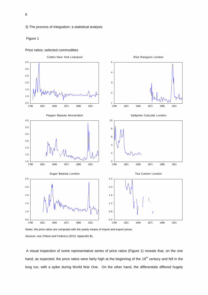
3) The process of integration: a statistical analysis

Figure 1

Price ratios: selected commodities

0.5

1.0

1.5

2.0

2.5

3.0

3.5

1796 1821 1846 1871 1896 1921

Cotton New York Liverpool

1

2

3

4

5

1796 1821 1846 1871 1896 1921

Rice Rangoon London

1.0

1.5

2.0

2.5

3.0

3.5

4.0

1796 1821 1846 1871 1896 1921

Pepper Batavia Amsterdam

0

2

4

6

8

10

1796 1821 1846 1871 1896 1921

Saltpetre Calcutta London

0.5

1.0

1.5

2.0

2.5

3.0

1796 1821 1846 1871 1896 1921

Sugar Batavia London

0.4

0.8

1.2

1.6

2.0

2.4

1796 1821 1846 1871 1896 1921

Tea Canton London

Notes: the price ratios are computed with the yearly means of import and export prices.

Sources: see Chilosi and Federico (2013: Appendix B).

A visual inspection of some representative series of price ratios (Figure 1) reveals that, on the one

hand, as expected, the price ratios were fairly high at the beginning of the 19th century and fell in the

long run, with a spike during World War One. On the other hand, the differentials differed hugely

7

among commodities at the same time (as seen in the vertical axis) and they often suddenly collapsed

rather than steadily declined.

More precise information on convergence can be obtained by estimating the equation (Razzaque et

al., 2007):

Δ Ln RPi=α + β TIME+ ψ ln RP

it-1+ φ ln Δ Ln RP

i t-1 +u 1)

Where RPi is the relative price of the i-th good between two markets and TIME is a linear trend. We

compute the long-run rate of change as t=- (β/ψ). The error correction model coefficient ψ (ranging

between -1 and 0) tests whether and estimates how rapidly price ratios return to this trend after a

shock, while the lagged change in relative prices is added to address possible serial correlation. We

first run Equation 1) as a fixed effects panel for the whole sample and separately by country,

considering jointly the (comparatively few) observations for the two Far Eastern countries, China and

Japan.

Table 3 Long-run convergence: panel estimation

N Initial ratio

Half-life (months)

Rate (in percentage)

Cumulated change (in

percentage)

All 1725 1.940 24 -0.443*** -46.72

Atlantic 257 1.618 20 -0.401*** -42.46

Far East 191 2.024 18 -0.520*** -52.22

India 805 2.085 26 -0.501*** -50.89

Indonesia 472 1.746 18 -0.402*** -37.25 Significant at * 10 per cent; ** 5 per cent; *** 10 per cent.

Notes: N=sample size. Fixed-effects estimation of equation 1) is used in all cases.

Sources: see Chilosi and Federico (2013: Appendix B).

The results (Table 3) confirm the conventional wisdom: at the beginning of the series (which differed

by product and route), European prices were on average double the Asian ones and by the end this

difference had been cut by a half. All rates are statistically significant and very similar across routes.

The half-lives of shocks are comparatively quite high. One might sum up that the market was

becoming increasingly integrated, but overall it had still a long way before becoming really efficient.

However, such a conclusion might be a tad hasty: it assumes stationary efficiency and linear price

convergence with equal rates by product. We explore difference in timing of integration by running

8

separate panel regressions for five periods: the twilight of mercantilism (1796-1815), the early

globalization (1815-1870), the heyday of globalization (1870-1913) and the war and interwar (1914-

1938). We also run for these periods a pooled group estimator, which allows rate of change to differ

across products and then averages them (Table 4).

Table 4 Trends by period: panel regression

N

Initial ratio

Half-life (months)

Rate (in percentage)

Cumulated change (in

percentage)

Pooled Group

estimator

Twilight of mercantilism (1796-1815)

All 102 2.274 10 0.968 20.20 1.920

Atlantic 27 1.215 9 3.249 62.81 4.855

India 72 3.099 9 0.285 17.00 -0.195

Early globalization (1815-1870)

All 565 1.973 16 -0.896*** -38.92 -0.759**

Atlantic 109 1.632 10 -0.678*** -31.12 -0.668***

Far East 48 2.245 12 -1.501** -55.55 -0.436

India 263 2.125 17 -1.243*** -49.51 -1.506***

Indonesia 145 1.892 12 -0.504** -21.48 0.235

Heyday of globalization (1870-1913)

All 765 1.291 8 -0.418*** -16.44 -0.379***

Atlantic 88 1.129 12 -0.288*** -11.65 -0.230

Far East 114 1.266 12 -0.334** -13.37 -0.235*

India 330 1.326 7 -0.517*** -19.95 -0.461*

Indonesia 233 1.311 8 -0.347*** -13.85 -0.359***

War and interwar (1914-1938)

All 313 1.441 10 -1.128*** -23.71 -1.116***

Atlantic 37 1.084 7 -0.160 -3.78 -0.260

Far East 27 1.157 0 -0.250* -5.82

India 150 1.559 10 -1.478** -28.86 -1.425***

Indonesia 99 1.483 9 -1.181** -24.69 -1.045**

Significant at * 10 per cent; ** 5 per cent; *** 10 per cent.

Notes: N=sample size. N=sample size. Fixed-effects estimation of equation 1) is used in all cases.

Sources: see Chilosi and Federico (2013: Appendix B).

As posited by the conventional wisdom, the results show no integration before 1815, although they

rely on a small and thus potentially non representative number of observations. The data for the two

subsequent periods are undoubtedly representative and they yield a clear conclusion: overall,

convergence was twice faster in the “early globalization” than during its (alleged) “heyday”. The

difference between the two periods is particularly wide for the Far East, while convergence between

Indonesia and Europe was only 45 per cent faster in 1815-1870 than in 1870-1913. Integration of

9

Indonesia during the “early globalization” is also the only case where the two estimators yield different

results. The negative coefficient(s) for the war and interwar period reflects the return to normal levels

of price differentials, after the sharp war-time increase. Indeed, dropping the first five years, the rates

become positive for the total and for all areas but the Far East. Yet the rates of inter-war disintegration

remain relatively small and are not statistically significant.2 In other words, the inter-war disintegration

of the world trading network affected little the Asian and American exports of primary products

analyzed here.

The increase in the speed of reaction between the second and third periods suggests an increase

in market efficiency. However, this is modest and the reaction remains rather slow: one may surmise

that in modern markets, most shocks were arbitraged away within the year and that, consequently,

our yearly series capture only very large shocks, which needed more time to be absorbed. This

conjecture should be tested with higher frequency data (Brunt and Cannon 2014).

One might suspect the inter-temporal comparisons to be biased by composition effects as the

coverage by product differs between periods. The absence of some bulky product from the panel

before 1870 implies a negative bias in the pace of integration during the “twilight of mercantilism”,

while the sample for the “heyday of globalization” includes high-value goods whose price differentials

were already very small by 1870 and could not fall further. We address this concern by running fixed-

effect panel regression of the natural logarithm of price ratio as a function of five year time dummies

(Bateman 2011).

2 The overall rate of change (in percentage) is 0.50 (not significant), while rates by area are -0.39 for the Far East (significant at

10 per cent), 0.63 for India, 0.53 for Dutch East Indies and 0.51 for the United States (none significant).

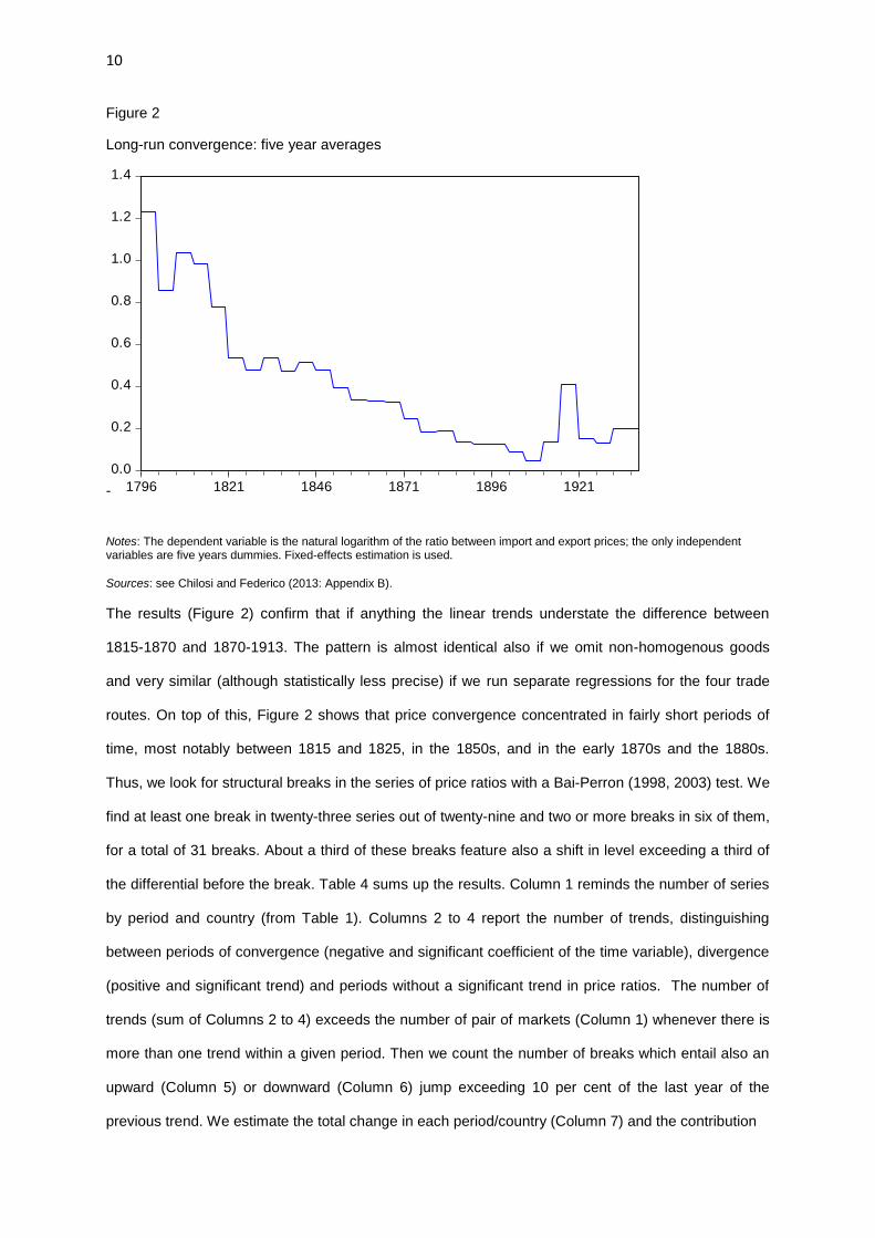
10

Figure 2

Long-run convergence: five year averages

-

0.0

0.2

0.4

0.6

0.8

1.0

1.2

1.4

1796 1821 1846 1871 1896 1921

Notes: The dependent variable is the natural logarithm of the ratio between import and export prices; the only independent variables are five years dummies. Fixed-effects estimation is used.

Sources: see Chilosi and Federico (2013: Appendix B).

The results (Figure 2) confirm that if anything the linear trends understate the difference between

1815-1870 and 1870-1913. The pattern is almost identical also if we omit non-homogenous goods

and very similar (although statistically less precise) if we run separate regressions for the four trade

routes. On top of this, Figure 2 shows that price convergence concentrated in fairly short periods of

time, most notably between 1815 and 1825, in the 1850s, and in the early 1870s and the 1880s.

Thus, we look for structural breaks in the series of price ratios with a Bai-Perron (1998, 2003) test. We

find at least one break in twenty-three series out of twenty-nine and two or more breaks in six of them,

for a total of 31 breaks. About a third of these breaks feature also a shift in level exceeding a third of

the differential before the break. Table 4 sums up the results. Column 1 reminds the number of series

by period and country (from Table 1). Columns 2 to 4 report the number of trends, distinguishing

between periods of convergence (negative and significant coefficient of the time variable), divergence

(positive and significant trend) and periods without a significant trend in price ratios. The number of

trends (sum of Columns 2 to 4) exceeds the number of pair of markets (Column 1) whenever there is

more than one trend within a given period. Then we count the number of breaks which entail also an

upward (Column 5) or downward (Column 6) jump exceeding 10 per cent of the last year of the

previous trend. We estimate the total change in each period/country (Column 7) and the contribution

11

Table 5

The four phases of globalization

Number of trends

Number of breaks

Total change in the period

Contribution of shocks

Implicit rate of change

Pairs of markets

Convergence Divergence Trendless Upward

shock Downward

shock (in percentage) (in percentage) (in percentage)

Twilight of mercantilism (1796-1815)

Atlantic 2

2

-1.10 0.00 -0.10

India 4

4

-3.50 0.00 -0.31

All 6

6

-2.70 0.00 -0.24

Early globalization (1815-1870)

Atlantic 2 1

2

2 -27.60 45.50 -0.45

Far East 3 1 1 2

1 -28.50 25.80 -0.79

India 8 4

5 1 5 -46.10 41.80 -1.90

Indonesia 5 3 1 3

2 -10.60 16.20 -0.47

All 18 9 2 12 1 10 -32.50 33.39 -1.20

Heyday globalization (1870-1913)

Atlantic 2

2

-8.40 21.40 -0.21

Far East 4 3 1 1

1 -2.80 5.70 -0.06

India 8 6 1 2 1 2 -19.30 22.70 -0.54

Indonesia 6 3

3

2 -14.30 41.30 -0.40

All 20 12 2 8 1 5 -13.40 24.76 -0.37

War and interwar (1914-1938)

Atlantic 2

2

-1.80 0.00 -0.08

Far East 1 1

-2.90 0.00 -0.12

India 8 4 2 2 3

1.80 17.50 0.28

Indonesia 4 1 1 2 2 1 4.90 43.50 0.16

All 15 6 3 6 5 1 1.84 20.91 0.17

Notes: The dependent variable in each regression is the natural logarithm of the ratio between import and export prices; the only independent variable is the time trend. The Bai-Perron (1998, 2003)

tests detect structural breaks in the constant and the slope. The total change and the implicit rate of change for each product in each period (Columns 7 and 9) are based on the formula Delta = (rpT-

12

Table 5-continued

rp0)/rp0, where Delta is the total change and the rps denote the fitted values at the end and beginning of the period. As at times

trends and shifts offset one another, to examine the extent to which cumulated changes are explained by them, we decompose

the sum of the absolute values of the predicted changes (Chilosi 2014), using the following formula: Delta_abs=|(rpn1-

rpn0)/rpn0|+|(rpn2-rpn1)*rpn1/(rpn1*rpn0)|+|(rpn3-rpn2)*rpn2/(rpn2*rpn0)|+… where rpni changes whenever there is a shift and again with

the new trend. In practice, there are at most two trends in each period (i.e. i=1, 2 or 3). The figures reported in Column 8 are

based on the proportions of Delta_abs explained by the shifts.

Sources: Chilosi and Federico (2013: table A1).

by shocks (Column 8), by averages of product specific figures. Last but not least, we compute an

overall trend, comparable with the linear trends of Table 4, as an average the product-specific yearly

rates of change (Column 9).

As a whole, our analysis confirms that convergence was consistently and significantly faster during

the “twilight of mercantilism” than during the “heyday of globalization”, although the difference for

Indonesia is very small. The analysis adds three important results. First, the timing of the breaks only

weakly supports the traditional periodization: slightly less than half of the breaks (14 out of 31) fall

within an interval of six years around 1815, 1870 or 1913 and almost as many (10) are farther than

ten years from these dates. Second, breaks mattered a lot. In the “twilight of mercantilism” phase, on

average, they accounted for one third of changes, as compared to a quarter during the “heyday” and

a fifth during the last period. Third, the timing of the breaks often coincided with important institutional

changes, detailed in the next section. Almost all the major shifts, 10 out of 12, clustered around 1815

or 1913 –, i.e. at the end of the EIC monopoly in Indian trade (1813) or at the outbreak of World War

One. One exception is the tea exported from Canton to London, whose price ratio saw a sudden fall

in 1835, two years after the demise of the EIC monopoly on that route; the other one is the sugar

exported from India, whose London price spiked up in 1839, after the ban on the import of West

Indian sugar cultivated by slaves. Moreover, the three negative shifts around 1870 are all from

Indonesia, where, as will be detailed in the next section, the monopoly on foreign trade was abolished

from 1868, considerably later than in India and China.3 By contrast, the Great Depression was

definitely not a shock in the market for primary products.

4) The causes of convergence: transport costs and barriers to trade

The conventional wisdom attributes the fall in the transaction costs of world trade before World War

One mostly to the combined effects of liberalization of trade and declines in transport costs;

3 The remaining shift near 1870 is positive and signals a slowing down in the pace of integration of linseed between Calcutta

and London. In fact, only in one case out of four does a structural break signal that the pace of integration increased after the 1870s (tin from Batavia).

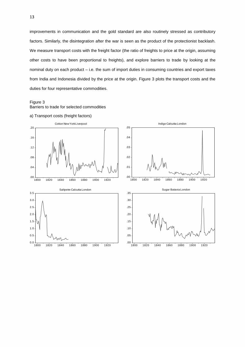
13

improvements in communication and the gold standard are also routinely stressed as contributory

factors. Similarly, the disintegration after the war is seen as the product of the protectionist backlash.

We measure transport costs with the freight factor (the ratio of freights to price at the origin, assuming

other costs to have been proportional to freights), and explore barriers to trade by looking at the

nominal duty on each product – i.e. the sum of import duties in consuming countries and export taxes

from India and Indonesia divided by the price at the origin. Figure 3 plots the transport costs and the

duties for four representative commodities.

Figure 3 Barriers to trade for selected commodities

a) Transport costs (freight factors)

.00

.04

.08

.12

.16

.20

1800 1820 1840 1860 1880 1900 1920.00

.01

.02

.03

.04

.05

1800 1820 1840 1860 1880 1900 1920

0.0

0.5

1.0

1.5

2.0

2.5

3.0

3.5

1800 1820 1840 1860 1880 1900 1920.00

.05

.10

.15

.20

.25

.30

.35

1800 1820 1840 1860 1880 1900 1920

Cotton New York Liverpool Indigo Calcutta London

Saltpetre Calcutta London Sugar Batavia London

14

Figure 3-continued

b) Import and export duties

Notes: the freight factors are equal to the nominal freights divided by the price at the origin. Similarly, the duties are equal to the

sum of import and export duties divided by the price at the origin.

Sources: see Chilosi and Federico (2013: Appendix B).

Levels are not directly comparable because the scales on the vertical axis differ, but trends are by

and large similar across countries and products. As expected, duties and freights did fall in the first

part of the 19th century, while, consistent with the results of Table 5, the rise in protection during the

Great Depression is very limited. From 1930 to 1938, total duties were on average equivalent to 26.8

per cent of the price in the exporting country, exceeding 50 per cent in 22 observations out of 95

(most of them on sugar). A fortiori, the impact of protection was limited over the whole period 1796-

1938: total duties exceeded 5 per cent of prices in slightly more than a quarter of cases and 50 per

cent only in about an eighth. On the same line, one should note that most of the fall in freights was

over by 1875 and that the change was often quite sudden. The 75 per cent collapse in the freight

factor for saltpetre in 1816-1817 is an extreme case, but there are several other instances of major

jumps, including a 70 per cent fall in freights for tea from China to England in 1835. Such sudden

.00

.02

.04

.06

.08

.10

.12

.14

.16

1800 1820 1840 1860 1880 1900 1920.00

.02

.04

.06

.08

.10

1800 1820 1840 1860 1880 1900 1920

0.0

0.2

0.4

0.6

0.8

1.0

1800 1820 1840 1860 1880 1900 19200

1

2

3

4

5

1800 1820 1840 1860 1880 1900 1920

Cotton New York London Indigo Calcutta London

Saltpetre Calcutta London Sugar Batavia London

15

changes cannot be accounted for by innovations in shipping organization or technology, the two

competing explanations for the fall in costs of sea transport (North, 1968; Harley, 1988; Shah and

Williamson, 2004), which by their nature are likely to spread gradually. Thus the evidence points to a

major role for the dismantling of the institutional barriers to Asian trade.

In Japan and China, these barriers were erected also by national governments to be dismantled by

the force of Western powers: Japan was forced to open to trade in 1854, while the restrictions to

Western merchants in China to trade in Canton only were lifted after the two opium wars in 1842 and

1858 (Dermigny 1964, Fairbank 1978, Wakeman 1978). The British East India Company (EIC)

enjoyed a monopoly on exports of Chinese tea to the United Kingdom and of imports of Indian opium

into China until 1833, when it ceased all its mercantile activities. The monopoly of trade between its

Indian possessions and the United Kingdom had been already abolished in July 1813. The Company

had traditionally paid very high freights, because it used large and heavily manned and armed ships

(Indiamen), very expensive to build and operate, which it rented from the owners. These were a small

group of Londoners, many of whom were also shareholders of the Company. Although the owners

were barred from participation in the Court of Directors since 1710, they infiltrated it with the ships’

husbands and captains, thus forming a cohesive oligopoly within the monopoly. According to the

conventional wisdom, the “shipping interest”, as it was known at the time, allowed the inflating of costs

and thus the circumvention of the Company’s official charter, which prevented it from earning extra-

profits from trade (Wakeman 1978, Mui and Mui 1984: 63-64, Bowen 2006: 252-256, Webster 2009:

32-40).4 Solar (2013) has recently suggested that the Indiamen were necessary to stave off the

military threat of competing Western trading companies. In his view freights collapsed in the 1810s

thanks to the combined effect of technical progress (mostly copper sheathing) and to the successes

of the Royal Navy, which made it possible to use smaller and cheaper ships. Anyway, since 1813

trade with India was free and in all likelihood the market was competitive. The expectation of great

profits from liberalized trade caused a glut in the market for transportation for India (Webster 2009:

72) and indeed our series of freight collapses in 1817.

The Dutch trade with its colonies in the Indian Ocean had been a monopoly of the Vereenigde Oost-

Indische Compagnie from the early 17th century to its bankruptcy in the 1790s. Trade remained free

4 The EIC charter stipulated that the price of company wares in London “should not exceed the prime cost, the freight and

charges of importation, the lawful interest of capital from the time of arrival of such tea in Britain, and the common premium in insurance" (Mui and Mui 1984: ix). Indeed, the official profits of the Company were quite low (Wakeman 1978: 167).

16

until 1825, when a monopoly on commerce with the Netherlands was granted to a new trading

company, the Nederlandsche Handel-Maatschappij, or NHM (Furnivall 1976, Horlings 1995: 142).

Similarly to the EIC, the company rented ships from Dutch owners, at “exceptionally high” rates

(Korthals Altes 1994: 161, Horlings 1995: 145). In its first years of activity, exports were reduced by a

rebellion of natives, the so called Java War. At the end of the war, the Dutch government, desperate

for revenues, established a system of compulsory delivery of coffee, sugar and indigo for exports,

known as Cultivation System (de Klerck 1938, Dobbin 1983, Fasseur 1992, Houben 2002, van

Zanden and Marks 2012). Peasants were paid much less than the world market price – about a half

of the Batavia price for coffee (Fasseur 1992: 37). The goods were transported to Amsterdam, and

there sold at auction: the profits, net of a fee for the NHM, accrued to the Dutch government. The

amount was very substantial: at its peak, in the 1850s, it accounted for over half the state revenues

and for about 3.8 per cent of Dutch GDP excluding any hidden subsidy to Dutch shipping and industry

(Smits et al. 2000, van Zanden and van Riel 2004). However, the Cultivation System was increasingly

unpopular at home and was slowly phased out. In 1850, the NHM liberalized the bidding contracts for

renting ships and its monopoly was abolished altogether in 1868 (NHM 1924: 23, Furnivall 1976: 168,

Korthals Altes 1994). The Dutch trade with the colonies remained free until 1918, when the sugar

producers set up a private association (VJSP) to allocate the scarce available shipping (van der Eng

1996: 215-216, Knight 2010). The organization continued to manage sugar exports after the end of

the war, and in 1932 it was substituted by a governmental organization (NIVAS) to manage sugar

production quotas under the international agreement (van der Eng 1996: 224-226). The Great

Depression featured also the first intervention in American agriculture: the Agricultural Adjustment Act

(AAA), part of the New Deal policies, established a loan facility for cotton farmers, which in practice

set a minimum price of cotton since 1934 (Federico and Sharp 2013).

5) The causes of integration: an econometric analysis

As implied by the preceding discussion, the ratio of prices for the i-th good (RPit) at time t can be

explained by the barriers to trade (B), the efficiency of markets (Em) and the transport costs (Tc)

Log RPit=F(B, Em, Tc) 2)

17

In our regression the set B includes the total duties (LOG_DUTY) and dummies for monopolies - a

dummy for the EIC (1796 to 1816) and separate dummies for the NHM under the full monopoly

regime (NHM1), from 1824 to 1850, and for the partially liberalized one (NHM2) from 1851 to 1868.5

We also add dummies for the AAA support to American cotton prices (since 1933) and for the two

marketing boards for Javanese sugar, the private VJSP (1918 to 1931) and the public NIVAS (after

1932). We expect duties and monopolies to increase price ratios, while the interventions on the

commodity market may augment or reduce price gaps according to the details of the policies.

Arguably the most important contribution to increasing market efficiency was the connection by

telegraph, which cut the time to transmit information from weeks to few minutes (Hoag 2006). The

cable between the United Kingdom and the United States was operational since 1866, and it was

followed four years later by the line to India and around 1875 by the line between Europe and

Indonesia (Headrick 1988: 101). We expect the TELEGRAPH dummy to be negative. We also add

dummies for a number of political events which may have disrupted the orderly working of markets,

such as the Java War in 1825-1827 (JAVA WAR), the Indian Mutiny in 1857-1859 (MUTINY), the

American Civil War (CIVIL WAR), the anti-slavery campaign, which boycotted Caribbean sugar, in

1840-1845 (SLAVE) and World War I (WWI).

By definition, the actual freights, the numerator of our measure of transport costs (LOG_FREIGHT),

include any rent paid to privileged Dutch or British ship-owners under the NHM and EIC monopoly

system. Consequently the EIC and NHM dummies measure only any additional effect of the trading

monopoly – e.g. from a manipulation of the market. We try to capture the total effect of monopoly,

including the rents to ship-owners by using an alternative series of freight factor

(LOG_FREIGHT_ADJ) net of the rents to shippers. We obtain this series (Figure 4) by scaling down

the actual series with coefficients from a fixed-effect panel regression, which explains freights with

dummies for the NHM and the EIC. By construction, the series move in parallel to LOG_FREIGHT,

except in the final year of the monopoly and thus the substitution affects the coefficient of transport

costs only marginally.

5 The variable LOG_DUTY is computed as log(1+t), where t is the ratio of (usually specific) duties to the price in the producing

country. It is thus zero if t=0. The dummy EIC is equal to 1 until 1816. We do not add a specific dummy for the end of the Napoleonic Wars because it would be collinear with the EIC dummy and it might bias the estimate of its coefficient. Anyway, price gaps with Asia in Britain were much less affected than in continental Europe by the Napoleonic Wars (O’Rourke 2006).

18

19

Figure 4 Freight factors and adjusted freight factors: selected commodities

i) Saltpetre Calcutta London

0.0

0.5

1.0

1.5

2.0

2.5

3.0

3.5

1796 1801 1806 1811 1816 1821 1826 1831 1836 1841

Freight factor

Adjusted freight factor

ii) Sugar Batavia London

.00

.04

.08

.12

.16

.20

.24

1823 1833 1843 1853 1863 1873 1883

Freight factor

Adjusted freight factor

Notes: The freight factor is the nominal freight rate divided by the price at the origin. The adjusted freight series are constructed by firstly running the regression LOG_FREIGHTit=c +αi+β1EICit+β2NHM1it+β3NHM2it+εit and secondly using the equation LOG_FREIGHT_ADJit=LOG_FREIGHTit-(β1EICit+β2NHM1it+β3NHM2it). Using alternative specifications, like including a time trend, yielded qualitatively identical results and only small quantitative differences.

Sources: see the text and Chilosi and Federico (2013: Appendix B).

20

We add the lagged value of the dependent variable to reduce auto-correlation and to take into

account the possible delay in adjustment to shocks, but its omission does not affect qualitatively the

results. The coefficients are thus short term elasticities; long run elasticities can be computed as βk/(1-

γ) where βk is the coefficient of the k-th variable and γ is the coefficient of the lagged dependent

variable.

The descriptive statistics for all variables and the pairwise coefficient of correlation between them do

not add much new information (Chilosi and Federico 2013). The correlation between explicative

variables is in general very low and thus there is no risk of multi-collinearity. On the other hand, most

variables are clearly non-stationary (cf. Chilosi and Federico 2013: Table A2, for a formal testing) and

thus results might be spurious. We therefore test ex-post the stationarity of the residuals with a Levin

et al. (2002) test for panel regressions.

Our analysis omits from the regression the Far Eastern markets, because the series are very short

and their quality is comparatively poor. This leaves a total of 22 cross-sections and 1568 observation.

As said before, we cannot categorically exclude that quality may be an issue for wheat (both from the

United States and from India), coffee sugar, pepper and tin (all from Indonesia). Thus, in Column 3 of

Table 6 we drop these products, reducing the coverage to 16 products and 1020 observations. Last

but not least, Indian trade, with 838 observations, is overrepresented in the sample. We address this

issue in two different ways. First, we run the regression with a restricted panel, featuring two products

per route (wheat and cotton for the United States, sugar e indigo for India, and pepper and sugar for

Indonesia), and we weight each of them with their share of the value of imports on that route. Thus,

in this specification (Table 6, Column 6), each route has the same weight on the results. Second, we

simply run separate regressions for the United States (Table 6, Column 7) India (Column 8) and

Indonesia (Column 9), which supply additional insights on the different causes of integration.

All regressions use fixed-effects specification with panel corrected standard errors to address cross-

sectional heteroskedasticity (reflecting different levels of transaction costs) and contemporaneous

correlation (which may arise from common shocks). Although we report results of an OLS estimate

(Tab 6, Column 1) for comparative purposes, we prefer to use instrumental variables because prices

in the exporting country appear in the denominator of the dependent variable and of two explicative

21

Table 6 The causes of integration

(1) (2) (3) (4) (5) (6) (7) (8) (9)

PCSE PCSE/IV PCSE/IV PCSE/IV PCSE/IV PCSE/IV PCSE/IV PCSE/IV PCSE/IV

C 0.517 0.365 0.327 0.366 0.329 0.224 0.312 0.386 0.416

(17.18)*** (8.73)*** (5.53)*** (8.73)*** (7.92)*** (4.48)*** (4.93)*** (5.51)*** (6.84)***

LOG_DUTY 0.084 0.051 0.048 0.051 0.033 0.039 0.13 0.021 0.057

(3.64)*** (2.03)** (0.87) (2.04)** (1.28) (1.31) (2.75)*** (0.32) (1.54)

EIC 0.173 0.236 0.253 0.345 0.287 0.347

0.343

(5.05)*** (6.30)*** (5.66)*** (9.98)*** (7.38)*** (7.04)***

(9.12)***

NHM1 -0.105 -0.044 -0.021 0.054 0.021 0.078

0.137

(-4.48)*** (-1.68)* (-0.22) (2.26)** (0.74) (2.37)**

(4.83)***

NHM2 -0.07 -0.046 0.013 0.023 -0.022 0.049

0.087

(-3.42)*** (-2.26)** (0.34) (1.04) (-1.05) (1.50)

(3.43)***

AAA 0.038 0.032 0.032 0.032 0.02 0.018 0.012

(0.79) (0.69) (0.67) (0.69) (0.46) (0.25) (0.28)

VJSP -0.079 -0.035

-0.035 -0.011 -0.011

-0.031

(-2.08)** (-0.90)

(-0.90) (-0.28) (-0.24)

(-0.78)

NIVAS -0.185 -0.125

-0.126 -0.105 -0.105

-0.153

(-3.61)*** (-2.35)**

(-2.35)** (-1.93)* (-1.60)

(-2.83)***

LOG_FREIGHT 0.123 0.067 0.053

0.085

(13.27)*** (4.64)*** (2.48)**

(3.65)***

LOG_FREIGHT_ADJ

0.067

0.034

0.068 0.073

(4.64)***

(2.01)**

(2.64)*** (4.44)***

LOG_FREIGHT*LIGHT

0.033

(2.14)**

LOG_FREIGHT*BULKY

0.108

(6.73)***

22

Table 6-continued

TELEGRAPH -0.043 -0.082 -0.095 -0.081 -0.083 -0.076 -0.017 -0.117 -0.046

(-2.57)** (-4.31)*** (-3.63)*** (-4.31)*** (-4.45)*** (-3.75)*** (-0.74) (-3.32)*** (-2.01)**

JAVA_WAR 0.064 0.063

0.063 0.072 0.071

0.066

(0.83) (0.80)

(0.80) (0.89) (0.86)

(0.82)

MUTINY -0.071 -0.066 -0.068 -0.066 -0.085 -0.060

-0.094

(-0.82) (-0.75) (-0.76) (-0.75) (-0.99) (-0.47)

(-1.06)

SLAVE 0.239 0.195 0.285 0.195 0.189 0.139

0.293 0.148

(5.62)*** (4.41)*** (4.91)*** (4.41)*** (4.20)*** (2.70)***

(4.98)*** (2.38)**

CIVIL_WAR -0.009 -0.055 -0.08 -0.055 -0.085 -0.082 -0.006

(-0.26) (-1.47) (-1.35) (-1.46) (-2.25)** (-1.61) (-0.15)

WWI*ATLANTIC -0.067 0.012 0.033 0.012 0.048 0.044 -0.034

(-1.23) (0.21) (0.55) (0.21) (0.92) (0.62) (-0.58)

WWI*INDIA 0.087 0.151 0.167 0.151 0.144 0.086

0.152

(2.08)** (3.40)*** (3.40)*** (3.40)*** (3.32)*** (1.14)

(2.93)***

WWI*INDONESIA 0.171 0.212 0.181 0.212 0.242 0.278

0.227

(5.67)*** (6.59)*** (4.34)*** (6.58)*** (7.09)*** (4.85)***

(7.27)***

LOG_RATIO1 0.445 0.497 0.513 0.496 0.463 0.452 0.503 0.51 0.338

(17.77)*** (18.00)*** (15.80)*** (18.00)*** (16.52)*** (12.11)*** (8.70)*** (14.90)*** (7.86)***

N 1534 1534 1020 1534 1534 619 231 821 482

Adjusted R-squared 0.79 0.78 0.79 0.78 0.79 0.64 0.76 0.79 0.76

F 153.67*** 129.36*** 120.24*** 129.37*** 129.61*** 49.38*** 77.07*** 133.66*** 76.88***

LLC t-stat -33.12*** -37.82*** -32.65*** -37.82*** -37.65*** -22.88*** -16.25*** -28.45*** -20.65***

Exogeneity chi-squared test

24.82*** 22.79*** 24.85*** 30.43*** 10.97*** 7.85** 20.20*** 7.70**

Exogeneity F test

12.90*** 12.90*** 12.83*** 11.31*** 3.81** 7.89*** 12.23*** 3.95**

Shea's partial R-squared 1st inst.

0.89 0.86 0.89 0.88 0.75 0.96 0.94 0.74

Shea's partial R-squared 2nd inst.

0.46 0.42 0.46 0.46 0.32 0.41 0.45 0.44

Shea's partial R-squared 3rd inst. 0.6

23

Table 6-continued

Significant at * 10 per cent; ** 5 per cent; *** 1 per cent.

Notes: PCSE=panel corrected standard errors; IV=instrumental variables estimation; N=sample size; inst.=instrument. The dependent variable in each regression is the natural logarithm of the ratio between import and export prices. Fixed-effects estimation with panel corrected standard errors is used in all cases; instrumental variable estimation for specifications (2) to (9); weighted least squares estimation for specification (6). Specification (3) includes only homogeneous goods; specification (6) includes only two goods per route; specifications (7) to (9) include only goods exported from the U.S., India and Indonesia, respectively.

Sources: see Chilosi and Federico (2013: Appendix B).

ones (duties and freights). Furthermore, freights might be endogenous in the short-run as well, if the

supply of shipping on those routes were inelastic (Jacks and Pendakur 2010). Specifically, we

instrument LOG_DUTY with the ratio of yearly duties to the average price throughout the whole period

– so that within variations depend only on the exogenous changes in specific duties. Likewise we use

average prices as denominator of the instrument for LOG_FREIGHT, while the numerator is the trend

component of a Hodrick-Prescott decomposition of the series of nominal freights.

The overall performance of the model is good. The residuals are stationary; the combined variables

are highly significant (F-test) and explain about four fifths of the total variance. Almost all the signs

agree with expectations. In all cases, the Wooldridge’s (1995) and the regression-based tests find

strong evidence of that the OLS estimates sufficiently differ from the instrumental variables’ ones to

recommend the use of the latter. All first stage tests find that the instruments are highly correlated

with the variables, so that the expected small-sample bias is low. Turning to the results:

i) As expected, the coefficients for freights are positive, highly significant and robust to the substitution

of monopoly-adjusted series (LOG_ ADJFREIGHT). A 10 per cent increase in freights augmented

price gaps by about 0.6-0.9 per cent in the short run and by about 1-1.5 per cent in the long run.

Moreover, as expected, the impact of costs is much bigger for bulky goods than for than for light

products; over three times, in fact (Column 5).6

ii) The variable LOG_DUTY is positive and significant in the baseline specification and its coefficient is

similar to the coefficient of freights. Indeed, the averages of the two variables are almost identical:

18.1 per cent for the freight factor and 18.2 per cent (17 per cent on imports and 1.2 per cent on

exports) for duties. Duties were high only on wheat, under the British Corn Laws before 1846, and

6 We run an OLS regression with LOG_FREIGHT as dependent variable, explained by a linear trend and by route and product

dummies. The product dummies yield a ranking of commodities from the lightest to the heaviest (silk, indigo, tin, cotton, tea, coffee, pepper, rubber, sugar, wheat, jute, saltpetre, linseed, rapeseed, and rice). We define ‘light’ the first nine products (“light”) and ‘bulky’ the others: this distinction closely mirrors the conventional one between “grain and seeds” and “lighter goods”.

24

sugar. In fact, the coefficient of LOG_DUTY is high and significant for the Atlantic trade (Column 7),

low and significant only at the 13 per cent level for Indonesia (Column 9) and very low and not

significant for India (Column 8).

iii) As expected, the monopoly of the British East India Company widened the price differentials, by a

quarter in the baseline specification with LOG_FREIGHT (Column 2) and by more than a third

(corresponding to a 70 per cent increase in the long run) if we add the effect of monopoly on freights

(Columns 4 and 7). In contrast, the NHM apparently fostered convergence both before (NHM1) and

after 1850 (NHM2). This effect however disappears if we use the monopoly-adjusted series of freights

(Columns 4 and 8). The NHM dummies become positive and significant, although the coefficients are

less than a quarter of the EIC one. In short, the NHM affected negatively long-range integration only

because it charged high freights, while it may have even increased the efficiency of the market, by

improving the transmission of information and by reducing the risks.7 In contrast, the monopoly of the

EIC harmed trade even discounting the effect on freights. The overall effect of state intervention after

World War One seems modest. Neither the Dutch (private) marketing board (VJSP) in the 1920s nor

the support to American agriculture after the Great Depression (AAA) affected significantly integration.

Only the Dutch public marketing board (the NIVAS) had a positive impact, reducing price gaps

between Indonesia and Europe by 10-15 per cent.

v) The variable TELEGRAPH is negative as expected and significant in all specifications.8 We have

tried to interact it with a time trend to capture the effect of technical progress and increases in

transmission (or changes in policy to set rates), but the results are poor. Our results confirm the

earlier work by Lew and Cater (2006) on the positive effect of telegraph on world trade.

vi)The political shocks in producing countries seem not to have affected international price

differentials, although of course they may have had important consequences in producing areas. In

contrast the campaign against slave-produced sugar in the United Kingdom (SLAVE) had a massive

7 An official history of the Company offers an alternative explanation of the negative signs in the baseline specifications: it

claims that the NHM sold at a loss to help Dutch middlemen to be competitive on the European market (NHM 1924: 18-19). 8We have tested separately three additional measures of efficiency: time trends, total traded quantity and a dummy for fixed

exchange rates between countries (i.e. the gold standard). All variables are expected negative. More trade should increase the flow of information, fixed exchange rates should reduce the risks of trading and time trends should capture all other improvements. The trends are significant only in Indonesia, but the variable is unexpectedly positive – i.e. ceteris paribus markets have been disintegrating. The quantity variable is negative, but it worsens the overall results of the regression (available upon request), probably because of endogeneity issues. The dummy for fixed exchange rate is incorrectly signed but not significant. Evidently, more refined measures of exchange rate volatility than afforded by the available data are needed to adequately capture the effect of exchange rate risk. The time trend is positive and significant for Indonesia – i.e. efficiency would have decreased, ceteris paribus. We speculate that the coefficient reflects the increasing exposure to price shocks originating in other markets.

25

effect on the sugar market. The dummies for WWI are positive and significant, as expected, for India

and Indonesia but not for the Atlantic. We interpret them as the effect of disruption in the market on

top of war-related increase in transport costs, which should already be captured by the variable

LOG_FREIGHT.

How much did each variable contribute to long run convergence? To answer, in Table 7 we report

the share of the total change accounted for by each variable.

Table 7 The causes of integration: decomposition analysis (in percentage)

(1) (2) (3) (4) (5) (6) (7)

Sample All All All All Atlantic India Indonesia

Years 1816-1913 1816-1870 1871-1913 1816-1913 1816-1913 1815-1913 1849-1913

EIC 39.27 49.57

57.25

69.14

NHM1

43.36

LOG_DUTY 4.65 5.56 1.14 4.65 42.11 1.72 2.98

LOG_FREIGHT 34.74 42.3 59.48

82.49

LOG_FREIGHT_ADJ

16.79

8.16 24.99

TELEGRAPH 20.34 15.8 37.3 20.31 13.08 23.47 14.6

Total 98.99 113.24 97.92 98.99 137.68 102.5 85.92

Notes: all the decompositions report the share of the percentage change in the dependent variable accounted for by each independent variable and are based on the results of the panel analysis presented in Table 6. Columns (1) to (3) are based on the second specification, Column (4) is based on the fourth specification, and Columns (5) to (8) are based on the seventh, eighth and ninth specifications, respectively. The exact starting date differs somewhat across samples in order to maximise the number of covered goods. We omit explicative variables which did not affect the dependent variables at the beginning and/or at the end of the period (such as the World War dummies). The cumulated change in the dependent variable is obtained as the average of the differences between the values fitted by the panel at time 0 and that of time T divided by the former. Sources: see the text and Chilosi and Federico (2013: Appendix B).

As the last row of Table 7 shows, the model performs very well: the divergence between the

cumulated effect of the variables and the actual change is less than 5 per cent in four cases and

exceeds 20 per cent only in the Atlantic trade. Most of the total convergence is explained by changes

in transportation costs and by the abolition of the EIC, which looms large in the long run analysis,

partly because the majority of observations in 1815 refer to India.9 According to the baseline

specification (Column 1), the fall in freights mattered almost as much, but this conclusion is decidedly

changed if we use the coefficient from LOG_FREIGHT_ADJS (Column 4). The NHM does not appear

9 But even if we give each route equal weight (i.e. using the sixth specification from table 6), the EIC emerges as by far the

most important factor, accounting for over 45 per cent of the overall decline.

26

among the variables in the aggregate analysis, because the series for Indonesia start later, but as

Column 7 shows, it played a very important role in the convergence of prices between the colony and

Europe, too. The telegraph did help a lot as well, accounting for between a sixth and a quarter of long-

run price convergence. In contrast, the cut in duties contributed substantially to the integration only in

the Atlantic economy (Column 5). The separate estimates by period (Columns 2 and 3) highlight the

sharp differences in the causes of integration. The “early globalization” was mostly determined by the

trade liberalization and the abolition of monopolies, while further convergence during the “heyday of

globalization” was achieved thanks to the lay-out of the telegraph lines and to fall in sea-borne

transport costs. On the whole, political decisions mattered more in the long run because, as shown in

section four, most of total convergence pre-dated 1870.

8) Conclusion

Our results are relevant for two literatures, that on market integration and that on trade and growth in

Asia, which, although clearly related, have so far remained largely distinct. Our work contributes to

filling in gaps in the literature on global market integration, strengthening the emerging consensus

view in the literature on Europe and the Atlantic trade. The process started early in the 19th century

and it was determined to a large extent by institutional changes. Within Europe and between Europe

and North America, barriers were raised essentially by protectionist trade policies, while commerce

with Asia was hampered by the monopoly of Western trading companies. These barriers were

progressively abolished and, at least for the sample of products/routes we are considering, were only

partially re-instated during the Great Depression. Once trade was free from institutional constraints,

further convergence was mainly achieved by cutting transportation costs. The cost of sea-borne trade,

however, was fairly low already at the beginning of the 19th century and thus the scope for further

convergence was limited.10

These findings are consistent with the view that market integration was at

the root of the terms of trade boom experienced by Asian countries in the decades before 1870.11

Future research should systematically assess this impact and examine the implications of market

integration for trade and welfare.

10

In contrast, transport costs from the producing areas to the ports were surely high and indeed there is a strong evidence of growing integration in the second half of the 19

th century in the domestic market in the United States (Federico and Sharp,

2013), in India (Hurd1975, Studer 2008, Andrabi and Kuehlwein 2010) and also in the Dutch East Indies (Marks 2010; van Zanden and Marks 2012: 25-26). Indeed, in a recent paper, Donaldson (2014) estimates that on average trade created by railways increased Indian GDP by as much as a sixth from 1870 to 1930.

11 This is particularly so as new estimates of terms of trade show that India took part in this boom, too (Chilosi and Federico

2013: 8).

27

References

Allen, R. C. (2011) Global Economic History. A Very Short Introduction. Oxford: Oxford University

Press.

Andrabi, T. and Kuehlwein, M. (2010) ‘Railways and price convergence in British India’, Journal of

Economic History 70, pp. 351-377.

Bai, J. and Perron, P. (1998) ‘Estimating and testing linear models with multiple structural changes’,

Econometrica, 66:1, pp. 47-78.

Bai, J. and Perron, P. (2003) ‘Computation and analysis of multiple structural change models’, Journal

of Applied Econometrics, 18, pp.1-22.

Bateman, V. N. (2011). ‘The evolution of markets in early modern Europe: a study of wheat prices,

1350-1800’, Economic History Review, 64, pp. 447-471.

Booth, A. (1988) Agricultural Development in Indonesia. Sidney: Allen and Unwin.

Bowen H.V. (2006) The Business of Empire. The East Company and Imperial Britain, 1756-1833.

Cambridge: Cambridge University Press.

Brandt, L., Ma, D. and Rawski, T. (2013) ‘From divergence to convergence: re-evaluating the history

behind China’s economic boom’, LSE Working Paper 175/13.

Broadberry, S. (2013) ‘Accounting for the Great Divergence’ LSE Economic History Working Paper

184/2013.

Brunt, L. and Cannon, E. (2014) ‘Integration in the English wheat market 1770-1820’ , Explorations in

Economic History, 52, pp. 111-130.

Chilosi, D. (2014) ‘Risky institutions: political regimes and the cost of public borrowing in early modern Italy’, Journal of Economic History, 74, pp. 886-914.

Chilosi, D. and Federico, G. (2013) ‘Asian globalizations: market integration, trade and economic growth, 1800-1938’ London School of Economics, Economic History Working Papers No: 183/2013

De Klerck, E. S. (1938) History of the Netherlands East Indies. Vol. 2. Rotterdam: Brusse.

Dermigny, L. (1964) La Chine et l’Occident. Le commerce a Canton au XVIIIe Siècle 1719-1833.

Tome III. Paris: SEVPEN.

Dobbin, C. (1983) Islamic Revivalism in a Changing Peasant Economy. Central Sumatra, 1784-1847.

London and Malmö: Curzon Press.

Donaldson, D. (2014). ‘Railroads and the Raj: Estimating the Economic Impact of Transportation

Infrastructure’, American Economic Review, forthcoming.

Dutt, R. (1969) The Economic History of India. Vols. 1-2, first ed. 1902-1904. New York: A. Kelley.

Fairbank, J. (1978) ‘The creation of the treaty system’, in Twitchett, D. and Fairbank, J. (eds.), The

Cambridge History of China. Vol 10, part I. Cambridge Cambridge University Press, pp. 213-264.

Fama, E. (1970) ‘Efficient capital markets: a review of theory and empirical work’, Journal of Finance,

25, pp. 383-417.

28

Fasseur, C. (1992) The Politics of Colonial Exploitation. Java, the Dutch and the Cultivation System.

Ithaca: South-East Asia Program Cornell University.

Federico, G. (2011) ‘When did the European market integrate?’ European Review of Economic

History, 15, pp. 93-126.

Federico, G. (2012) ‘How much do we know about market integration in Europe?’, Economic History

Review, 65: 2, pp. 470-497.

Federico, G. and Sharp, P. (2013) ‘The Cost of railroad regulation: the disintegration of American

agricultural markets in the interwar period’, Economic History Review, 66, pp. 1017-1038.

Federico, G. and Tena, A. (2013) ‘World trade 1800-1938’, paper presented to the Seventh World Cliometric Conference (Hawaii).

Feuerwerker, A. (1980) ‘Economic trends in the late Ch’ing Empire, 1870-1911’, in Fairbank, J. and Liu, K. (eds.), The Cambridge History of China. Vol. 11, part II. Cambridge: Cambridge University Press, pp.1-69.

Feuerwerker, A. (1983) ‘Economic trends,1912-1949’, in Fairbank, J. (ed.), The Cambridge History of China. Vol. 12, part I. Cambridge: Cambridge University Press, pp. 28-127.

Furnivall, J. S. (1976) Netherlands India. A Study of a Plural Economy. Reprint. Amsterdam: Israel.

Harley, K. (1988) ‘Ocean freight rates and productivity, 1740-1913: the primacy of mechanical invention reaffirmed’, Journal of Economic History, 48, pp. 851-876.

Headrick, D. (1988) The Tentacles of Progress. Technology Transfer in the Age of Imperialism, 1850-1940 Oxford: Oxford University Press.

Horlings, E. (1995) The Economic Development of the Dutch Service Sector, 1800-1850. Amsterdam:

NEHA.

Hoag Christopher (2006) ‘The Atlantic cable and capital market information flows’, Journal of

Economic History, 66, pp. 342-353

Houben, V. J.H. (2002) ‘Java in the 19th century: consolidation of a territorial state’ in Dick, H.,

Houben, V. J. H., Lindblad J. T. and Wie, T. K. (eds.) The Emergence of a National Economy. An

Economic History of Indonesia, 1800-2000. Crows Nest and Honolulu: Allen & Unwin and University

of Hawai’i Press, pp. 56-81.

Hynes W., Jacks, D. S. and O’Rourke, K. H. (2012) ‘Commodity market disintegration in the interwar

period’, European Review Economic History, 16, pp.119-143.

Hurd, J. (1975) ‘Railways and the expansion of markets in India, 1861-1921’, Explorations in Economic History, 12, pp. 263-288.

Jacks, D. S. (2005) ‘Intra – and international commodity market integration in the Atlantic economy’,

Explorations in Economic History, 42, pp. 381-413.

Jacks, D. S. and Pendakur, K. (2010) ‘Global trade and the maritime transport revolution’, Review Economics and Statistics, 92, pp. 745-755.

Knight , R. (2010) ‘Exogenous colonialism: Java sugar between Nippon and Taikoo before and during the interwar depression, c. 1920–1940’, Modern Asian Studies, 44, pp. 477-515. Korthals Altes, W.L. (1994) Changing Economy in Indonesia vol. 15 Prices (non Rice) 1814-1940.

The Hague: Royal Tropical Institute.

29

Levin, A., Lin, C. F. and Chu, C. (2002). ‘Unit root tests in panel data: asymptotic and finite-sample

properties’, Journal of Econometrics, 108, pp. 1–24.

Lew, B. and Cater, B. (2006) ‘The telegraph, co-ordination of tramp shipping and growth in world

trade 1870-1910’, European Review of Economic History, 10, pp.147-173.

Maddison Project (2013) At www.ggdc.net/maddison/maddison-project/data.htm.‎ Accessed on

January 25th 2013.

Marks, D. (2010) ‘Unity or diversity? On the integration and efficiency of rice markets in Indonesia,

c.1920-2006’, Explorations in Economic History, 47, pp. 310-324.

Mui, H. and Mui, L. H. (1984) The Management of Monopoly. A Study of the English East India Company's Conduct of its Tea Trade, 1784-1833. Vancouver: University of British Columbia Press. Nederlandsche Handel-Maatschappij (1924) A Brief History of the Netherlands Trading Society, 1824-1924. The Hague: Mouton & Company. North, D. C. (1968) ‘Sources of productivity change in ocean shipping, 1600-1850’, Journal of Political Economy, 76, pp. 953-970.

O’Rourke, K. H. (2006). ‘The worldwide economic impact of the French Revolutionary and Napoleonic Wars, 1793-1815’, Journal of Global History, 1, pp. 123-149.

O’Rourke, K. H. and Williamson, J. G. (2002) ‘When did globalization begin?’, European Review of

Economic History, 6, pp. 23-50.

Parthasarathi, P. (2011) Why Europe Grew Rich and Asia Did Not. Global Economic Divergence,

1600-1850. Cambridge: Cambridge University Press.

Pomeranz, K. (2000) The Great Divergence. Europe, China and the Making of the Modern World Economy. Princeton: Princeton University Press.

Razzaque, M. Osafa-Kwaako, P. and Grynberg, R. (2007) ‘Long-run trend in the relative price:

empirical estimation for individual commodities’ in Grynberg, R. and Newton, S. (eds) Commodity

Prices and Development. Oxford University Press Oxford 2007 pp. 35-67.

Rönnbäck, K. (2009) ‘Integration of global commodity markets in the early modern era’, European

Review of Economic History, 13, pp. 95-120.

Roy, T. (2000) The Economic History of India, 1857-1947. Oxford: Oxford University Press. Sachs, J. and Warner, A. M. (2001), ‘Natural resources and economic development: the curse of natural resources’, European Economic Review, 45, pp. 827-838.

Shah, M., and Williamson, J. G. (2004) ‘Freight rates and productivity gains in British tramp shipping 1869-1950’, Explorations in Economic History, 41, pp.174-203.

Sharp, P. and Weisdorf, J. (2013) ‘Globalization revisited: market integration and the wheat trade

between North America and Britain from the eighteenth century’, Explorations in Economic History,

50, pp.88-98.

Smits, J.P., Horlings, E. and van Zanden, J. L. (2000) The Measurement of Gross National Product

and its Components, 1800-1913 (Groningen Growth and Development Centre Monograph series no 5

2000, data available at http://nationalaccounts.niwi.knaw.nl/, accessed in January 2009).

Solar, P.M. (2013) ‘Opening to the East. Shipping between Europe and Asia, 1780-1830’, Journal of Economic History, 73, pp. 625-661.

30

Studer, R. (2008) ‘India and the great divergence: assessing the efficiency of grain markets in 18

th

and 19th century India’, Journal of Economic History, 68, pp. 393-437.

Tomlinson, B. R. (1993) The Economy of Modern India, 1860-1970. Cambridge: Cambridge University Press. Uebele, M. (2011) ‘National and international market integration in the 19th century: evidence from comovement’, Explorations in Economic History, 48, pp. 226–242.

Van der Eng, P. (1996) Agricultural Growth in Indonesia. London and Basingstoke: Macmillan.

Van Zanden, J. L. and van Riel, A. (2004) The Strictures of Inheritance. The Dutch Economy in the

Nineteenth Century. Princeton: Princeton University Press.

Van Zanden, J. L. and Marks, D. (2012) An Economic History of Indonesia, 1800-2010. London and

New York: Routledge.

Wakeman, F. (1978) ‘The Canton trade and the Opium war’ in Twitchett, D. and Fairbank, J. (eds.),

The Cambridge History of China. Vol. 10, part I. Cambridge: Cambridge University Press, pp.163-212.

Webster, A. (2009) The Twilight of the East India Company. Woodbridge: Boydell Press.

Wooldridge, J. M. (1995) ‘Score diagnostics for linear models estimated by two stage least squares’.

In Maddala, G. S., Phillips, P. C. B. and Srinivasan, T. N. (eds.) Advances in Econometrics and

Quantitative Economics: Essays in Honor of Professor C. R. Rao. Oxford: Blackwell, pp.66-87.

Williamson, J. G. (2008) ‘Globalization and the great divergence: terms of trade boom, volatility and the poor periphery, 1782-1913’, European Review of Economic History, 12:3, pp. 355-391.

Williamson, J. G. (2011) Trade and Poverty. When the Third World Fell Behind. Cambridge, Mass.:

MIT Press.

Williamson, J. G. (2012) ‘Commodity prices over two centuries: trends, volatility, and impact’, Annual Review of Resource Economics, 4, pp. 185-206.

Williamson, J. G. (2013) ‘The commodity export, growth, and distribution connection in Southeast Asia 1500-1940’, paper presented to the Southeast Asian Economic Growth Conference (Bangkok).