Dataflow Execution for Reliability and Performance on ... · Ao colega e amigo Leandro Marzulo pela...

DATAFLOW EXECUTION FOR RELIABILITY AND PERFORMANCE ON

CURRENT HARDWARE

Tiago Assumpcao de Oliveira Alves

Tese de Doutorado apresentada ao Programa

de Pos-graduacao em Engenharia de

Sistemas e Computacao, COPPE, da

Universidade Federal do Rio de Janeiro,

como parte dos requisitos necessarios a

obtencao do tıtulo de Doutor em Engenharia

de Sistemas e Computacao.

Orientador: Felipe Maia Galvao Franca

Rio de Janeiro

Maio de 2014


CURRENT HARDWARE


TESE SUBMETIDA AO CORPO DOCENTE DO INSTITUTO ALBERTO LUIZ

COIMBRA DE POS-GRADUACAO E PESQUISA DE ENGENHARIA (COPPE)

DA UNIVERSIDADE FEDERAL DO RIO DE JANEIRO COMO PARTE DOS

REQUISITOS NECESSARIOS PARA A OBTENCAO DO GRAU DE DOUTOR

EM CIENCIAS EM ENGENHARIA DE SISTEMAS E COMPUTACAO.

Examinada por:

Prof. Felipe Maia Galvao Franca, Ph.D.

Prof. Valmir Carneiro Barbosa, Ph.D.

Prof. Claudio Esperanca, Ph.D.

Prof. Renato Antonio Celso Ferreira, Ph.D.

Prof. Sandip Kundu, Ph.D.

RIO DE JANEIRO, RJ – BRASIL

MAIO DE 2014

Alves, Tiago Assumpcao de Oliveira

Dataflow Execution for Reliability and Performance on

Current Hardware/Tiago Assumpcao de Oliveira Alves. –

Rio de Janeiro: UFRJ/COPPE, 2014.

XII, 94 p.: il.; 29, 7cm.


Tese (doutorado) – UFRJ/COPPE/Programa de

Engenharia de Sistemas e Computacao, 2014.

Referencias Bibliograficas: p. 87 – 94.

1. Programacao Paralela. 2. Sistemas de Multiplos

Nucleos. 3. Arquitetura de Computadores. I. Franca,

Felipe Maia Galvao. II. Universidade Federal do Rio de

Janeiro, COPPE, Programa de Engenharia de Sistemas e

Computacao. III. Tıtulo.

iii

Agradecimentos

Gostaria de agradecer ao meu orientador Felipe Franca por todo apoio durante o

mestrado e o doutorado. Sua confianca na minha capacidade foi essencial para o

sucesso deste trabalho.

Aos meus pais e irma por me darem todo o suporte necessario para que eu

pudesse trilhar este caminho. Sem voces seria impossıvel.

Ao colega e amigo Leandro Marzulo pela parceria de anos. Espero que contin-

uemos essa colaboracao de sucesso por um bom tempo.

Ao professor Sandip Kundu por me receber e orientar na UMass. Ao professor

Valmir Barbosa por ser um modelo de pesquisador no qual sempre procuro me

espelhar.

Obrigado as agencias de fomento CAPES e FAPERJ pelas bolsas que recebi

durante o doutorado.

iv

Resumo da Tese apresentada a COPPE/UFRJ como parte dos requisitos necessarios

para a obtencao do grau de Doutor em Ciencias (D.Sc.)

EXECUCAO GUIADA PELO FLUXO DE DADOS PARA CONFIABILIDADE E

DESEMPENHO EM HARDWARE ATUAL


Maio/2014


Programa: Engenharia de Sistemas e Computacao

Execucao dataflow, onde instrucoes podem comecar a executar assim que seus

operandos de entrada estiverem prontos, e uma maneira natural para se obter par-

alelismo. Recentemente, o dataflow tornou a receber atencao como uma ferramenta

para programacao paralela na era dos multicores e manycores. A mudanca de foco

em direcao ao dataflow traz consigo a necessidade de pesquisa que expanda o con-

hecimento a respeito de execucao dataflow e que adicione novas funcionalidades

ao espectro do que pode ser feito com dataflow. Trabalhos anteriores que estu-

dam o desempenho de aplicacoes paralelas se focam predominantemente em grafos

acıclicos dirigidos, um modelo que nao e capaz de representar diretamente aplicacoes

dataflow. Alem disso, nao ha nenhum trabalho anterior na area de deteccao e re-

cuperacao de erro cujo alvo seja execucao dataflow. Nesta tese introduzimos as

seguintes contribuicoes: (i) algoritmos de escalonamento estatico/dinamico para

ambientes dataflow ; (ii) ferramentas teoricas que nos permitem modelar o desem-

penho de aplicacoes dataflow ; (iii) um algoritmo para detecao e recuperacao de

erros em dataflow a (iv) um modelo para execucao GPU+CPU que incorpora as

funcionalidades de GPU ao grafo dataflow. Nos implementamos todo o trabalho in-

troduzido nesta tese em nosso modelo TALM dataflow e executamos experimentos

com essas implementacoes. Os resultados experimentais validam o nosso modelo

teorico para o desempenho de aplicacoes dataflow e mostram que as funcionalidades

introduzidas atingem bom desempenho.

v

Abstract of Thesis presented to COPPE/UFRJ as a partial fulfillment of the

requirements for the degree of Doctor of Science (D.Sc.)


CURRENT HARDWARE


May/2014

Advisor: Felipe Maia Galvao Franca

Department: Systems Engineering and Computer Science

Dataflow execution, where instructions can start executing as soon as their in-

put operands are ready, is a natural way to obtain parallelism. Recently, dataflow

execution has regained traction as a tool for programming in the multicore and

manycore era. The shift of focus toward dataflow calls for research that expands the

knowledge about dataflow execution and that adds functionalities to the spectrum

of what can be done with dataflow. Prior work on bounds for the performance of

parallel programs mostly focus on DAGs (Directed Acyclic Graphs), a model that

can not directly represent dataflow programs. Besides that, there has been no work

in the area of Error Detection and Recovery that targets dataflow execution. In

this thesis we introduce the following contributions to dataflow execution: (i) novel

static/dynamic scheduling algorithms for dataflow runtimes; (ii) theoretical tools

that allow us to model the performance of dynamic dataflow programs; (iii) an al-

gorithm for error detection and recovery in dataflow execution and (iv) a model for

GPU+CPU execution that incorporates GPU functionalities to the dataflow graph.

We implemented all the work introduced in our TALM dataflow model and executed

experiments with such implementations. The experimental resuls validate the theo-

retical model of dataflow performance and show that the functionalities introduced

in this thesis present good performance.

vi

Contents

List of Figures ix

1 Introduction 1

2 Related Work 4

2.1 Dataflow-based Programming Models . . . . . . . . . . . . . . . . . . 4

2.1.1 Auto-Pipe . . . . . . . . . . . . . . . . . . . . . . . . . . . . . 4

2.1.2 StreamIt . . . . . . . . . . . . . . . . . . . . . . . . . . . . . . 5

2.1.3 Intel Threading Building Blocks . . . . . . . . . . . . . . . . . 6

2.2 Static Scheduling . . . . . . . . . . . . . . . . . . . . . . . . . . . . . 6

2.3 Work-Stealing . . . . . . . . . . . . . . . . . . . . . . . . . . . . . . . 7

3 TALM 10

3.1 Instruction Set . . . . . . . . . . . . . . . . . . . . . . . . . . . . . . 10

3.2 Super-instructions . . . . . . . . . . . . . . . . . . . . . . . . . . . . . 15

3.3 Trebuchet: TALM for multicores . . . . . . . . . . . . . . . . . . . . 17

3.3.1 Virtual Machine Implementation . . . . . . . . . . . . . . . . 17

3.3.2 Parallelising Applications with Trebuchet . . . . . . . . . . . . 18

3.3.3 Global termination detection . . . . . . . . . . . . . . . . . . . 21

3.4 Describing Pipelines in TALM . . . . . . . . . . . . . . . . . . . . . . 22

3.5 THLL (TALM High Level Language) . . . . . . . . . . . . . . . . . . 22

3.6 Instruction Placement and Work-Stealing . . . . . . . . . . . . . . . . 24

3.6.1 Placement Assembly Macros . . . . . . . . . . . . . . . . . . . 24

3.6.2 Couillard Naive Placement . . . . . . . . . . . . . . . . . . . . 26

3.6.3 Static Placement Algorithm . . . . . . . . . . . . . . . . . . . 26

3.7 Static Scheduling . . . . . . . . . . . . . . . . . . . . . . . . . . . . . 26

3.8 Work-Stealing . . . . . . . . . . . . . . . . . . . . . . . . . . . . . . . 28

3.8.1 Selective Work-Stealing . . . . . . . . . . . . . . . . . . . . . . 31

3.9 Dynamic Programming with Dataflow . . . . . . . . . . . . . . . . . 34

3.9.1 Longest Common Subsequence . . . . . . . . . . . . . . . . . . 37

3.9.2 Dataflow LCS Implementation . . . . . . . . . . . . . . . . . . 38

vii

3.9.3 LCS Experiments . . . . . . . . . . . . . . . . . . . . . . . . . 39

4 Concurrency Analysis for Dynamic Dataflow Graphs 45

4.1 Definition of Dynamic Dataflow Graphs . . . . . . . . . . . . . . . . . 46

4.2 Maximum Degree of Concurrency in a DDG . . . . . . . . . . . . . . 47

4.2.1 Proof of Correctness . . . . . . . . . . . . . . . . . . . . . . . 51

4.3 Average Degree of Concurrency (Maximum Speed-up) . . . . . . . . . 53

4.4 Lower Bound for Speed-up . . . . . . . . . . . . . . . . . . . . . . . . 55

4.5 Static Scheduling Algorithm Optimization . . . . . . . . . . . . . . . 56

4.6 Example: Comparing different Pipelines . . . . . . . . . . . . . . . . 56

4.7 Experiments . . . . . . . . . . . . . . . . . . . . . . . . . . . . . . . . 57

4.8 Eliminating the Restrictions of DDGs . . . . . . . . . . . . . . . . . . 63

5 Dataflow Error Detection and Recovery 65

5.1 Dataflow Error Detection and Recovery . . . . . . . . . . . . . . . . . 67

5.1.1 Error Detection . . . . . . . . . . . . . . . . . . . . . . . . . . 67

5.1.2 Error Recovery . . . . . . . . . . . . . . . . . . . . . . . . . . 67

5.1.3 Output-Commit Problem . . . . . . . . . . . . . . . . . . . . . 68

5.1.4 Domino Effect Protection . . . . . . . . . . . . . . . . . . . . 68

5.1.5 Error-free input identification . . . . . . . . . . . . . . . . . . 69

5.2 Benchmarks . . . . . . . . . . . . . . . . . . . . . . . . . . . . . . . . 71

5.2.1 Longest Common Subsequence (LCS) . . . . . . . . . . . . . . 71

5.2.2 Matrices Multiplication (MxM) . . . . . . . . . . . . . . . . . 71

5.2.3 Raytracing (RT) . . . . . . . . . . . . . . . . . . . . . . . . . 71

5.3 Performance Results . . . . . . . . . . . . . . . . . . . . . . . . . . . 72

5.4 Comparison with Prior Work . . . . . . . . . . . . . . . . . . . . . . 72

6 Support for GPUs 76

6.1 GPU support in TALM . . . . . . . . . . . . . . . . . . . . . . . . . . 77

6.2 Computation Overlap . . . . . . . . . . . . . . . . . . . . . . . . . . . 79

6.3 Concurrency Analysis of a GPU application . . . . . . . . . . . . . . 79

6.4 Experimental Results . . . . . . . . . . . . . . . . . . . . . . . . . . . 82

7 Discussion and Future Work 84

Bibliography 87

viii

List of Figures

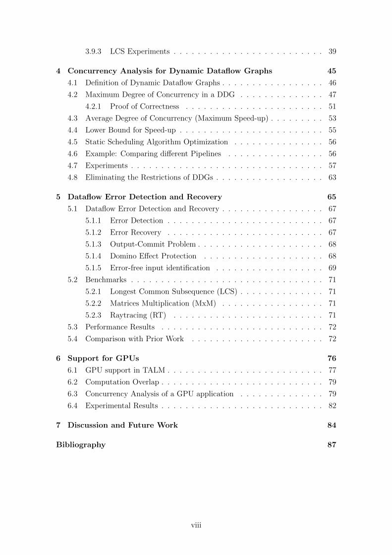
2.1 Example of a pipeline that can not be represented in TBB. In (a)

the original pipeline and in (b) the modified version that complies

with the restriction imposed by TBB. The original pipeline can not

be implemented because TBB does not support non-linear pipelines.

The workaround introduced for the modified version limits the par-

allelism, since A and B will never execute in parallel, although they

potentially could because there is no dependency between them. . . . 6

3.1 Instruction Format at TALM. . . . . . . . . . . . . . . . . . . . . . . 11

3.2 Assembly Example . . . . . . . . . . . . . . . . . . . . . . . . . . . . 14

3.3 TALM Architecture. . . . . . . . . . . . . . . . . . . . . . . . . . . . 16

3.4 Trebuchet Structures. . . . . . . . . . . . . . . . . . . . . . . . . . . . 17

3.5 Work-flow to follow when parallelising applications with Trebuchet. . 19

3.6 Using Trebuchet. . . . . . . . . . . . . . . . . . . . . . . . . . . . . . 20

3.7 Example of a complex pipeline in TALM . . . . . . . . . . . . . . . . 23

3.8 Example of THLL sourcecode. . . . . . . . . . . . . . . . . . . . . . . 25

3.9 Dataflow graph corresponding to the THLL code in Figure 3.8 . . . . 25

3.10 Data structure corresponding to a deque. The anchors for the owner

and for one thief are represented. The shaded positions in the array

represent tasks that were already visited by the thief thread. . . . . . 32

3.11 Structures used in the Selective Work-Stealing Algorithm. . . . . . . 34

3.12 Finding the Levenshtein Distance between two strings X =

〈F,B,C,G,E〉 and Y = 〈A,B,C,D,E,G,E〉 with LCS. The Lev-

enshtein Distance between X and Y is 4 and, in this case, there is

only one longest common subsequence between X and Y (〈B,C,G,E〉). 41

3.13 Longest Common Subsequence Dependency Graph. Complete de-

pendence graph, where each element depends on its upper, left and

upper-left neighbors is shown in (a). Dependency Graph after re-

moving transitive dependencies is shwon in (b). . . . . . . . . . . . . 42

ix

3.14 TALM Dataflow Implementation of LCS Application. Pane A shows

TALM code that describe the graph. The graph itself is shown at pane

B. This solution allows elimination of barriers and unleashes paral-

lelism in the wavefront. Dataflow triggers task execution according

to data dependencies. Notice that all synchronization is distributed,

there are no global barriers. . . . . . . . . . . . . . . . . . . . . . . . 43

3.15 OpenMP versus Dataflow. Speedups are shown on y-axis and number

of cores on x-axis. Performance gains up to 23% were obtained with

Dataflow execution. . . . . . . . . . . . . . . . . . . . . . . . . . . . 44

4.1 Example of DDGs whose maximum degree of concurrency are 1, 2

and unbounded, respectively. The dashed arcs represent return edges. 48

4.2 Example of unrolling a DDG. Instructions b , c, d and e are inside

a loop (observe the return edge) and a is just an initialization for

the loop. The loop is unrolled twice, and the edges (d(0), b(1)) and

(d(1), b(2)) are added to represent the dependency caused by the re-

turn edge. . . . . . . . . . . . . . . . . . . . . . . . . . . . . . . . . . 51

4.3 Example of execution of the second iteration of the algorithm (k = 1).

In (a) we have the original DDG, in (b) the DAG obtained by unrolling

it once and in (c) we have the complement-path graph. The maximum

degree of concurrency is 2, since it is the size of the maximum cliques. 52

4.4 Example corresponding to a loop that executes for n iterations. In (a)

we present the DDG and in (b) the DAG tha represents the execution. 54

4.5 Example of execution of Algorithm 4.1 in which the maximum con-

currency converges. . . . . . . . . . . . . . . . . . . . . . . . . . . . . 57

4.6 Example of execution of Algorithm 4.1 in which the maximum degree

of concurrency does not converge. . . . . . . . . . . . . . . . . . . . 58

4.7 DDG that describes the TALM implementation of Ferret, considering

that the number of available PEs is 3. The three instructions in

the middle are the instances of the parallel super-instruction that

implements the second stage of the pipeline. . . . . . . . . . . . . . . 59

4.8 Results for the original version of Ferret. The shaded area represents

the potential for speed-up between Smax and Smin. Smax does not

vary with the number of PEs. Static/Dynamic are the results for the

execution that utilized both static and dynamic scheduling, Dynamic

Only is the execution with just work-stealing, Smax is the upper bound

for speed-up and Smin the lower bound. . . . . . . . . . . . . . . . . . 60

x

4.9 Results for the modified version of Ferret with iteration-dependent

similarity search stage. Smax varies with the number of PEs due to

the variation in super-instruction granularity. Since the middle stage

is split among the PEs used, the granularity of that super-instruction

is reduced, which in turn reduces the critical path length. Also, at

some point the granularity of the middle stage becomes so fine that

the critical path becomes the first stage, like in the original version.

This explains abrupt changes in the lines. . . . . . . . . . . . . . . . . 62

4.10 Results for the modified version of Ferret with iteration-dependent

similarity search stage. Smax varies with the number of PEs due to

the variation in super-instruction granularity. Since the middle stage

is split among the PEs used, the granularity of that super-instruction

is reduced, which in turn reduces the critical path length. Also, at

some point the granularity of the middle stage becomes so fine that

the critical path becomes the first stage, like in the original version.

This explains abrupt changes in the lines. . . . . . . . . . . . . . . . . 63

5.1 TALM assembly code transformation to add error detection. In (b)

we have the original graph (without error-detection) and in (d) the

transformed code with the redundant tasks (tAcopy, tBcopy, tCcopy

and tDcopy) and the commit instructions. Figures (a) and (c) are

visual representations of the two versions. . . . . . . . . . . . . . . . 69

5.2 Example where wait edges (labeled with w) are necessary to pre-

vent unnecessary re-executions. The redundant tasks are omitted for

readability, but there are implicit replications of A, B and C. . . . . . 71

5.3 Error Detection Performance Analysis for MxM and Raytracing. The

chart shows overhead information when varying the number of par-

allel primary tasks (2, 4, 6 and 12). For the MxM application results

also show the overheads when using ”Domino Effect Protection” (ED

vs ED-DEP). Each bar details the overheads of task execution, con-

trol instructions, commit instructions, send and receive operations

(communication) and idle time. . . . . . . . . . . . . . . . . . . . . . 73

5.4 Error Detection Performance Analysis for LCS . . . . . . . . . . . . . 73

6.1 TALM architecture with GPU support. Each PE is responsible for

one GPU. The illustrated system has N PEs but only two GPUs

available. . . . . . . . . . . . . . . . . . . . . . . . . . . . . . . . . . . 77

6.2 Example of TALM assembly code using the GPU support. The use of

the asynchronous instructions cphtodev and cpdevtoh causes com-

putation overlap. . . . . . . . . . . . . . . . . . . . . . . . . . . . . . 80

xi

6.3 Example of execution of an application that can take advantage of

asynchronous operations in order to overlap CPU computation with

GPU communication/computation. In the diagram on the top, the

execution with the computation overlap and in the diagram in the

bottom the same computation with all synchronous operations. Here

HDi, Ki, DHi and OUTi correspond to the i − th iteration’s host

to gpu (device) copy, kernel call, gpu to host copy and output super-

instruction, respectively. . . . . . . . . . . . . . . . . . . . . . . . . . 81

6.4 Example of execution in a GPU with one queue for each type of

operation. Operations from different iterations overlap. . . . . . . . . 81

6.5 DDG that represents the pattern of execution of Figure 6.4. . . . . . 82

6.6 Performance results for the comparison of a CUDA only implemen-

tation and a Trebuchet with GPU support version (TrebGPU) of the

same application. The TrebGPU version performs 30% better because

implementing the application as a dataflow graph allowed Trebuchet

to exploit communication/computation overlap. . . . . . . . . . . . . 83

xii

Chapter 1

Introduction

Dataflow execution, where instructions can start executing as soon as their input

operands are ready, is a natural way to obtain parallelism. Recently, dataflow execu-

tion has regained traction as a tool for programming in the multicore and manycore

era [1], [2], [3]. The motivation behind the adoption of dataflow as a programming

practice lies in its inherent parallelism. In dataflow progamming the programmer

just has to annotate the code indicating the dependencies between the portions of

code to be parallelized and then compile/execute using a dataflow toolchain. This

way, the dataflow runtime used will be able to execute in parallel portions of code

that are independent, if there are resources available, lightening the burden of syn-

chronization desing on the programmer, who in this case will not have to rely on

complex structures like semaphores or locks.

The shift of focus toward dataflow calls for research that expands the knowledge

about dataflow execution and that adds functionalities to the spectrum of what can

be done with dataflow. In this thesis we propose a series of algorithms and techniques

that enable dataflow users to model the performance of dataflow applications, obtain

better static/dynamic scheduling, achieve error detection/recovery and implement

dataflow programs using GPUs.

In order to exploit parallelism using dataflow it is necessary to use either a spe-

cialized library or runtime that is responsible for dispatching tasks to execution

according to the dataflow rule. These tools bring overhead to program execution,

since it is necessary to execute extra code to achieve dataflow parallelization. Ide-

ally these overheads should be minimum, but that is not the case in most real world

scenarios. Thus, it is necessary to come up with techniques that allow us to in-

fer the amount of overhead a dataflow library or runtime is imposing on program

execution. In this thesis we developed a model of computation that allows us to

study the potential performance in programs to be parallelized using dataflow. By

comparing experimental results of actual executions with the theoretical model for

the parallelism of a dataflow program, we can evaluate the impact of the overheads

1

of the dataflow library or runtime in the performance.

Having a model for the concurrency of dataflow programs not only helps us

predict the potential performance but also can allow us to allocate resources accord-

ingly. For instance, if the data dependencies in a program only allow it to execute

at most two tasks in parallel, it would be potentially wasteful to allocate more than

two processors to execute such program. Taking that into consideration, we have

devised an algorithm that utilizes the aforementioned model of computation to ob-

tain the maximum degree of concurrency (the greatest number of tasks/instructions

that can execute in parallel at any time) of a program.

One other important aspect to be considered when addressing issues related to

parallel programming is that as the number of processors grows, the probability

of faults occurring in one of the processors also increases. Consider the case of

transient errors, which are faults in execution that occur only once due to some

external interference. This kind of error can cause the program to produce incorrect

outputs, since the program may still execute to completion in case a transient error

ocurrs. These faults are specially critical in the scope of high performance computing

(HPC), since HPC programs may run for long periods of time and an incorrect

output detected only at the end of the execution may cause an enormous waste of

resources. In addition to that, it may be the case that it is just not possible to

determine if the output data is fautly or not, since the program may exit gracefully

in the presence of a transient error. In such cases the only way to verify the data

would be to re-execute the entire program to validate the output, which is obviously

an inefficient approach.

To address this issues we have developed an algorithm for online error detection

and recovery in dataflow execution. Although there is prior work on error detection

and recovery, there has been no work that deals with these issues in the field of

dataflow execution. Our approach takes advantage of the inherent parallelism of

dataflow to develop a completely distributed algorithm that provides error detection

and concurrency. Basically, we add the components for error detection and recovery

to the dataflow graph, which guarantees parallelism within the mechanism itself and

between the mechanism and the program.

In this work we also propose a model for GPU computing within a dataflow

environment. We believe that extending the functionalities represented by dataflow

graphs with the support for GPU can allow us to obtain CPU/GPU parallelism in an

intuitive manner, just like the proposed approach for error detection and recovery.

Also, as we will show, by adding the GPU functinalities to the dataflow graph we

are able to exploit our concurrency analysis techniques to model the performance of

programs with complex CPU/GPU computation overlap schemes.

In prior work we have introduced TALM [4, 5], a dataflow execution model that

2

adopts dynamic dataflow to parallelize programs. We have implemented a complete

toolchain comprising a programming language (THLL), a compiler (Couillard) and

a runtime for multicore machines (Trebuchet). In this thesis we used TALM to ex-

periment with our techniques, but our work can be applied to any dynamic dataflow

system.

The main contributions of this thesis are the following:

• A static scheduling algorithm based on List Scheduling that takes in consid-

eration conditional execution, which is an important characteristic of TALM

and dataflow in general.

• A novel work-stealing algorithm that allows the programmer to specify a

heuristic to determine what instructions should be stolen.

• A study of how to parallelize dynamic programming algorithms using dataflow.

• A model of computation and techniques for concurrency analysis of dynamic

dataflow applications.

• A model for transient error detection and recovery in dataflow.

• Support for GPU programming in TALM, along with an example of how to

apply the analysis techniques to applications that use CPU+GPU.

3

Chapter 2

Related Work

This chapter presents prior work that is related to the work introduced in this

thesis. We subdivide prior work into the following sections: (i) Dataflow-based Pro-

gramming Models; (ii) Static Scheduling; (iii) Work-Stealing and (iv) Concurrency

Analysis. For clarity, we left the discussion about prior work on Error Detection

and Recovery to Chapter 5.

2.1 Dataflow-based Programming Models

Applications with streaming patterns have become increasingly important. Describ-

ing streams in imperative programming languages can be an ardous and tedious

task due to the complexity of implementing the synchronizationh necessary to ex-

ploit parallelism. Basically, the programmer will have to manually establish (with

locks or semaphores) the communication between the pipeline stages that comprise

the stream. Most of the dataflow based programming models were created with fo-

cus on streaming programming, motivated by its inherent difficulties. This section

discusses some of these models.

2.1.1 Auto-Pipe

Auto-Pipe [6] is a set of tools developed to ease the development and evaluation

of applications with pipeline pattern. The pipelines implemented in Auto-Pipe are

designed to be executed on heterogeneous architectures, comprised by diverse com-

putational resources such as CPUs, GPUs and FPGAs.

As we mentioned, implementing pipelines in standard imperative languages can

be quite complex. Thus, programming models that intend to facilitate pipeline

implementation must also provide a specific promming language for that purpose,

besides the other tools used in the devolpment and execution. Auto-Pipe is com-

prised by the following components:

4

• The X language, used to specify a set of coarse-grained tasks that are to be

mapped to the different computational resources of the heterogenous archi-

tecture. The code that implements the functionalities of each task must be

implemented in CUDA, C or VHDL, depending on the computational resources

to which the task is going to be mapped.

• A compiler for the X language that integrates the blocks (tasks) in the specified

topology and the architecture.

• The simulation environment that allows the programmer to verify the correct-

ness and performance of applications devoloped in VHDL (targeting FPGAs)

and in C language.

• A set of pre-compiled tasks, loadable bitmaps for FPGAs and interface mod-

ules. Together, these subprograms are responsible for the integration of tasks

mapped to different computational resources.

In Auto-Pipe a program is a set of block instances, implemented in C, VHDL or

CUDA. These blocks are put together using the X language, forming a pipeline, and

in the instantiation of each block the programmer must specify the target platform

of each block (i.e. CPU, GPU or FPGA), so that that Auto-Pipe can decide how to

compile/synthesize each block. Since Auto-Pipe targets heterogenous architectures,

each block must be compiled according to the resource in which it will be executed.

In a separate file, the programmer describes the computational resources that com-

prise the system and the block to resource mapping, specifying where each block

will be executed.

2.1.2 StreamIt

StreamIt [7] is a domain specific language designed for streaming programming ap-

plications, such as filters, compression algorithms etc. The basic unit in StreamIt are

filters (implemented using the Filter class). StreamIt is based on object oriented

programming, filters are created via inheritance from the Filter class. Each filter

must have a init() and a work() methods, responsible for the filter initialization

and process, respectively. These filter objects are then instantiated and connected

in the Main class. Filter-to-filter connection in StreamIt can follow three patterns:

Pipeline, SplitJoin and FeedbackLoop.

A set of benchmarks for StreamIt was proposed in [8]. As opposed to TBB

[9], StreamIt allows non-linear pipelines. However, it does not allow pipelines with

conditional execution, i.e. it is not possible to have a stage in the pipeline that may

not be executed, depending on some boolean control. As we shall see in Chapter 3,

this is perfectly possible in our model.

5

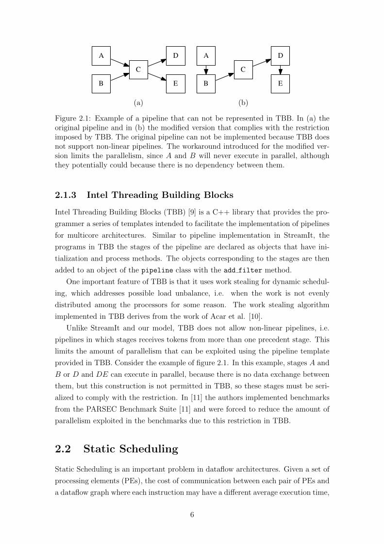
A

C

D

EB

A

C

B

D

E

(a) (b)

Figure 2.1: Example of a pipeline that can not be represented in TBB. In (a) theoriginal pipeline and in (b) the modified version that complies with the restrictionimposed by TBB. The original pipeline can not be implemented because TBB doesnot support non-linear pipelines. The workaround introduced for the modified ver-sion limits the parallelism, since A and B will never execute in parallel, althoughthey potentially could because there is no dependency between them.

2.1.3 Intel Threading Building Blocks

Intel Threading Building Blocks (TBB) [9] is a C++ library that provides the pro-

grammer a series of templates intended to facilitate the implementation of pipelines

for multicore architectures. Similar to pipeline implementation in StreamIt, the

programs in TBB the stages of the pipeline are declared as objects that have ini-

tialization and process methods. The objects corresponding to the stages are then

added to an object of the pipeline class with the add filter method.

One important feature of TBB is that it uses work stealing for dynamic schedul-

ing, which addresses possible load unbalance, i.e. when the work is not evenly

distributed among the processors for some reason. The work stealing algorithm

implemented in TBB derives from the work of Acar et al. [10].

Unlike StreamIt and our model, TBB does not allow non-linear pipelines, i.e.

pipelines in which stages receives tokens from more than one precedent stage. This

limits the amount of parallelism that can be exploited using the pipeline template

provided in TBB. Consider the example of figure 2.1. In this example, stages A and

B or D and DE can execute in parallel, because there is no data exchange between

them, but this construction is not permitted in TBB, so these stages must be seri-

alized to comply with the restriction. In [11] the authors implemented benchmarks

from the PARSEC Benchmark Suite [11] and were forced to reduce the amount of

parallelism exploited in the benchmarks due to this restriction in TBB.

2.2 Static Scheduling

Static Scheduling is an important problem in dataflow architectures. Given a set of

processing elements (PEs), the cost of communication between each pair of PEs and

a dataflow graph where each instruction may have a different average execution time,

6

the problem consists on assingning instructions to PEs in compile time. Mercaldi

et al. [12] proposed eight different strategies for static scheduling in the WaveScalar

architecture [13]. Since the WaveScaler architecture is a hierarchical grid of PEs,

the focus in [12] is to take advantage of the hierarchy of the communication in

the grid. Since the cost of the communication between two PEs depends on where

they are located in the grid, these strategies aim at mapping instructions that have

dependencies between them to PEs that are as close as possible.

Sih et al. [14] presented a heuristic that improves the traditional list scheduling

algorithm in architectures with limited or irregular interconnection structures. Their

approach adds a dynamic factor to the priority given to instructions during the

scheduling process. Thus, at each iteration of the scheduling algorithm, the priority

of each of the instructions that are yet to be mapped depend not only on the

characteristics of the graph, but also on the instructions that were already mapped

at that point, this way instructions that exchange data are more likely to be mapped

close to one another.

Topcuoglu et al. [15] presented an approach similar to [14]; Their algorithm

also splits the priority given to instructions into two parts: static, based solely

on characteristics of the graph, and dynamic, based on estimations obtained using

the set of instructions that were mapped in previous iterations of the scheduling

algorithm. One key advantage of this approach is that it tries to fill empty slots

between instructions that were already mapped. If two instructions were mapped

to a PE and there is an empty slot between them, typically because the second one

needs to wait for data from its predecessors, the algorithm will try to place a third

instruction between the two.

Boyer and Hurra [16] introduced an algorithm that also derives list scheduling.

The main difference is that in their algorithm the next instructino the be scheduled is

chosen randomly between the instructions whose predecessors have all been mapped

at that point. Due to its randomness, the algorithm is executed multiple times,

always maintaining the best result obtained so far, until a criteria is met. This

criteria can be either the maximum number of executions or the lack of change in the

best solution found, i.e. the same result being obtained after numerous executions.

2.3 Work-Stealing

If the load unbalancing issue remains untreated, the system can only achieve good

performance in applications where the computation is uniformly distributed among

processing elements. In many cases, obtaining such even distribution of load is not

possible, either because the application dynamically creates tasks or because the

execution times of functions in the program are data-dependent, which makes them

7

unpredictable at compile-time.

Applications with pipeline pattern may have stages that execute slower than the

others, which can cause the PEs to which the faster stages were mapped to become

idle. If there is no load balancing mechanism, the programmer may be forced to

coalesce the stages in the pipeline to avoid this effect. Although this would mantain

data parallelism, task parallelism would be lost.

Relagating the task of implementing load balancing to the programmer may not

be a good decision, because of the complexity of such task. Thus, it is usually

more interesting to have load balancing implemented in the parallel programming

library or runtime transparent to the user. In our work we focus on work-stealing

approaches, mainly because of the lack of a central scheduler in such approaches,

which tends allow better scalability. Besides, since static scheduling is also a topic to

be studied in this work, work-stealing is a better match for dynamic scheduling, as it

only interferes with the execution when there is load unbalancing. If load was evenly

distributed by static scheduling, work-stealing will never be activated because PEs

will not become idle, hence its suitability to be applied in conjunction with static

scheduling.

Arora et al. [17] the introduced the algorithm that is still considered the state

of the art in work-stealing because of its rigorously proven good performance. The

algorithm is based on concurrent data structures called double ended queues (or

deques), which are queues that can be accessed by both ends. Each thread has its

own deque and it accesses the deque (both to push and to pop work) from one end

while the neighbor threads that want to steal work, called thieves, access it from the

other end. Since thieves access the deque from a different end, they are less likely

to interfere with the owner of the deque and this is a good way to prioritize the

owner’s operations on the deque. The synchronization on the deque is done via the

Compare-and-Swap (CAS) atomic operation. This algorithm was implemented in

several major parallel programming projects, such as Cilk [18] and Intel Threading

Building Blocks [9]. One significant shortcoming of the algorithm proposed in [17]

is that the size of the deques can not change during execution.

Chase and Lev [19] proposed a variation on Arora’s algorithm that allowed the

deque to shrink or grow, solving the problem of the fixed size. Is this new algorithm,

deques are implemented as circular arrays and new procedures to extend or reduce

the size of such arrays were introduced.

It is important to notice that, although it may reduce CPU idle time, work-

stealing may cause loss of data locality. In the algorithms mentioned above the

“victim” deque from which a thread tries to steal work is chosen randomly, hence

the possibility of stealing work that might cause cache pollution, since the data

already in the cache of the thief is not taken in consideration. Acar et al. [10]

8

introduced a variation to the algorithm of Arora et al. that employed the use of

structures called mailboxes. Each thread has its own mailbox which other threads

will use to send spawned tasks that have affinity with the thread that owns the

mailbox. The threads will thus prioritize stealing tasks that are on their mailboxes

instead of just randomly looking for tasks to steal. The key disadvantage of this

approach is that it adds another level of synchronization, since one task can appear

in mailboxes and in a deque, which makes it more complicated to assure that only

one thread will execute that task.

Another issue that must be taken into consideration is the choice of to which

mailboxes to send each task created. In [10] the authors proposed that the program-

mer should use code annotations to inform the runtime the data set on which each

task operates, thus enabling the runtime to detect affinity between created tasks and

threads. On the other hand, Guo et al. [20] proposed a work-stealing algorithm that

also uses mailboxes but does not require assistance from the programmer. In [20],

threads are grouped together in sets called places, according the memory hierarchy

of the target architecture, and each of these places has a separate mailbox that is

shared by the threads that belong to it. This way, threads will prioritize stealing

work from the mailboxes of the places to which they belong, which makes it more

likely that the data read by the stolen task is in the cache shared by threads in that

place.

9

Chapter 3

TALM

Predominantly, computer architectures, both mono and multiprocessed, follow the

Von Neumann model, where the execution is guided by control flow. In spite of being

control flow guided, techniques based on the flow of data, namely the Tomasulo

Algorithm, have been widely adopted as a way of exploiting ILP in such machines.

These techniques, however, are limited by the instruction issue, which happens in

order, so portions of code may only execute in parallel if there is proximity between

them in sequential order, even if there is no data dependency.

TALM (TALM is an Architecture and Language for Multithreading), which was

introduced in [21], is model for parallel programming and execution based in the

dataflow paradigm. Due to TALM’s flexibility, it was chosen to serve as base for the

implementation and experiments of the techniques proposed in this work. In this

chapter we will provide an overall description of TALM.

3.1 Instruction Set

The primary focus of TALM is to provide an abstraction so that applications can

be implemented according to the dataflow paradigm and executed on top of a Von

Neumann target architecture. It is then essential to have flexible granularity of in-

structions (or tasks) in the model, so that granularity can be adjusted according

to the overheads of the TALM implementation for each target architecture. This

problem is address by the adoption of super-instructions, instructions that are im-

plemented by the programmer to be used along with simple (fine grained) dataflow

instructions. This way, when developing a parallel program, the programmer will

use his own super-instructions to describe a dataflow graph that implements the

application. As stated, it is important to keep in mind the overheads of the TALM

implementation for the target architecture when deciding the granularity of the

super-instructions.

Since instruction granularity may vary, it is important that the way instructions

10

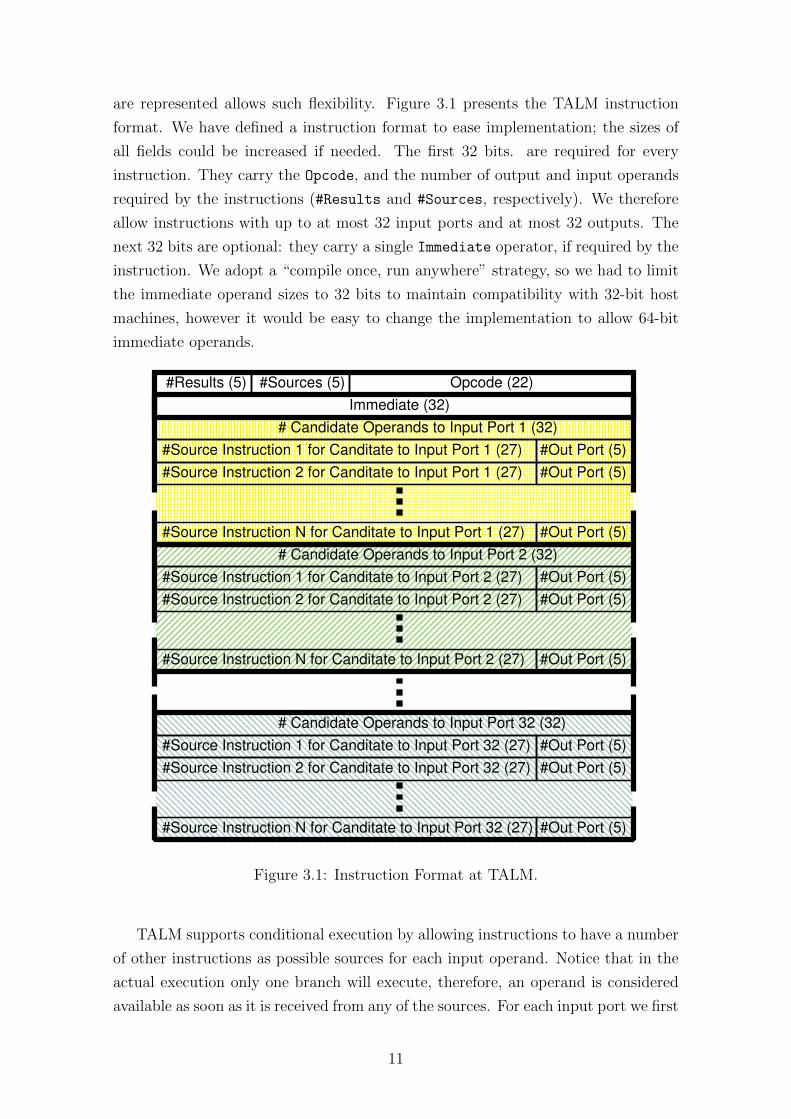
are represented allows such flexibility. Figure 3.1 presents the TALM instruction

format. We have defined a instruction format to ease implementation; the sizes of

all fields could be increased if needed. The first 32 bits. are required for every

instruction. They carry the Opcode, and the number of output and input operands

required by the instructions (#Results and #Sources, respectively). We therefore

allow instructions with up to at most 32 input ports and at most 32 outputs. The

next 32 bits are optional: they carry a single Immediate operator, if required by the

instruction. We adopt a “compile once, run anywhere” strategy, so we had to limit

the immediate operand sizes to 32 bits to maintain compatibility with 32-bit host

machines, however it would be easy to change the implementation to allow 64-bit

immediate operands.

#Results (5) #Sources (5) Opcode (22)

# Candidate Operands to Input Port 1 (32)

#Source Instruction 1 for Canditate to Input Port 1 (27) #Out Port (5)

#Source Instruction 2 for Canditate to Input Port 1 (27)

#Source Instruction N for Canditate to Input Port 1 (27)

Immediate (32)

#Out Port (5)

#Out Port (5)





#Out Port (5)

#Out Port (5)





#Out Port (5)

#Out Port (5)

Figure 3.1: Instruction Format at TALM.

TALM supports conditional execution by allowing instructions to have a number

of other instructions as possible sources for each input operand. Notice that in the

actual execution only one branch will execute, therefore, an operand is considered

available as soon as it is received from any of the sources. For each input port we first

11

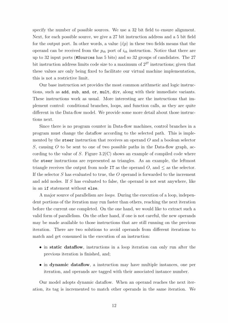
specify the number of possible sources. We use a 32 bit field to ensure alignment.

Next, for each possible source, we give a 27 bit instruction address and a 5 bit field

for the output port. In other words, a value 〈i|p〉 in these two fields means that the

operand can be received from the pth port of ith instruction. Notice that there are

up to 32 input ports (#Sources has 5 bits) and so 32 groups of candidates. The 27

bit instruction address limits code size to a maximum of 227 instructions; given that

these values are only being fixed to facilitate our virtual machine implementation,

this is not a restrictive limit.

Our base instruction set provides the most common arithmetic and logic instruc-

tions, such as add, sub, and, or, mult, div, along with their immediate variants.

These instructions work as usual. More interesting are the instructions that im-

plement control: conditional branches, loops, and function calls, as they are quite

different in the Data-flow model. We provide some more detail about those instruc-

tions next.

Since there is no program counter in Data-flow machines, control branches in a

program must change the dataflow according to the selected path. This is imple-

mented by the steer instruction that receives an operand O and a boolean selector

S, causing O to be sent to one of two possible paths in the Data-flow graph, ac-

cording to the value of S. Figure 3.2(C) shows an example of compiled code where

the steer instructions are represented as triangles. As an example, the leftmost

triangle receives the output from node IT as the operand O, and ≤ as the selector.

If the selector S has evaluated to true, the O operand is forwarded to the increment

and add nodes. If S has evaluated to false, the operand is not sent anywhere, like

in an if statement without else.

A major source of parallelism are loops. During the execution of a loop, indepen-

dent portions of the iteration may run faster than others, reaching the next iteration

before the current one completed. On the one hand, we would like to extract such a

valid form of parallelism. On the other hand, if one is not careful, the new operands

may be made available to those instructions that are still running on the previous

iteration. There are two solutions to avoid operands from different iterations to

match and get consumed in the execution of an instruction:

• in static dataflow, instructions in a loop iteration can only run after the

previous iteration is finished, and;

• in dynamic dataflow, a instruction may have multiple instances, one per

iteration, and operands are tagged with their associated instance number.

Our model adopts dynamic dataflow. When an operand reaches the next iter-

ation, its tag is incremented to match other operands in the same iteration. We

12

choose to implement dynamic dataflow, as parallelism is our main goal and our im-

plementation is software-based. The Increment Iteration Tag (inctag) instruction

is responsible for separating different iterations of different loops. Instructions will

execute once they have received a complete set of input operands with the same tag.

Figure 3.2(C) represents inctag instructions as circular nodes labeled IT. Notice for

example how the rightmost steer and inctag nodes interact to implement a loop:

when the condition ≤ evaluates as true, the steer nodes forward their arguments to

the inctag nodes, allowing execution to move on to the next iteration. Eventually,

the condition fails and the outputs of inctag nodes are forwarded to the ret node,

discussed next.

In TALM, functions are blocks of instructions that can receive operands (param-

eters) from different call sites in the code. We call such callsites static. Moreover,

the same callsite may run multiple times, for example, when it is in a loop or in

the case of recursive functions. We call such callsites dynamic. We follow the same

approach used for loops, providing a way to identify operands from different static

and dynamic call sites so that they only match with operands belonging the same

execution of the function. Thus, a call tag is also added to the operand, containing:

• the call group, generated at assembly time by the preprocessor, through the

callgroup macro, and it identifies different static callsites.

• the call instance number, which identifies dynamic instances from the same

callsite.

The call group is an integer number stored at the immediate field of callsnd instruc-

tions. The call instance number is updated dynamically, based on a local counter

(CallCounter) of the callsnd instruction. When a function is called, callsnd in-

structions will be used to send input operands (or parameters), with the call tag,

to the function being called. The caller’s call tag is also sent to the callee (with the

retsnd instruction) to be used when the function returns a value to the caller. In

that case, the call tag in the return operand must be restored to match the caller’s.

This is done by the ret instruction.

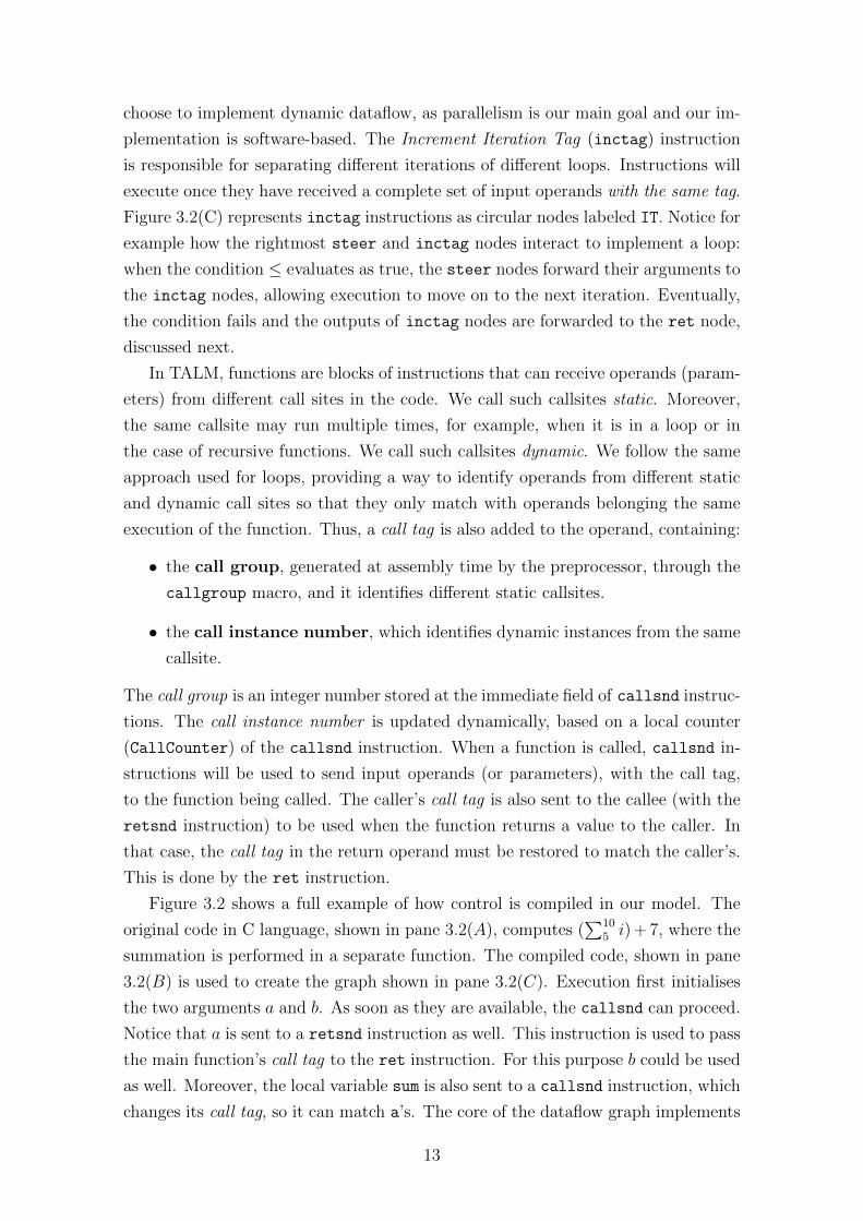
Figure 3.2 shows a full example of how control is compiled in our model. The

original code in C language, shown in pane 3.2(A), computes (∑10

5 i) + 7, where the

summation is performed in a separate function. The compiled code, shown in pane

3.2(B) is used to create the graph shown in pane 3.2(C). Execution first initialises

the two arguments a and b. As soon as they are available, the callsnd can proceed.

Notice that a is sent to a retsnd instruction as well. This instruction is used to pass

the main function’s call tag to the ret instruction. For this purpose b could be used

as well. Moreover, the local variable sum is also sent to a callsnd instruction, which

changes its call tag, so it can match a’s. The core of the dataflow graph implements

13

void main() { int a=5, b=10; x=summation(a,b)+7;}

int summation (int a, int b) { int i, sum=0; for (i=a;i<=b;i++) sum+=i; return sum;}

A

const a, 5const b, 10const sum, 0callgroup("c1", "summation")callsnd sa, a, c1callsnd sb, b, c1callsnd ssum, sum, c1retsnd retid, a, c1addi x, summation.c1, 7inctag iloop, [sa, ai]inctag sloop, [ssum, sumres]inctag bloop, [sb, stb.t]inctag retloop, [retid, stret.t]lteq comp, iloop, bloopsteer sti, comp, iloopsteer stsum, comp, sloopsteer stb, comp, bloopsteer stret, comp, retloopaddi ai, sti.t, 1add sumres, stsum.t, sti.tret summation, stsum.f, stret.f

B

ab

callsnd

#c1

callsnd

#c1sum

IT

ret

+

IT

T F

IT

<=

+1

+7

C

retsnd

#c1

callsnd

#c1 IT

T F T F T F

Figure 3.2: Assembly Example

14

the loop: notice that parallelism in the graph is constrained by the comparison ≤;

on the other hand, the graph naturally specifies the parallelism in the program, and

in fact portions of the loop body might start executing a new iteration even before

other other instructions of the body finish the previous one.

3.2 Super-instructions

In accordance with the goal of TALM to provide an abstraction for dataflow pro-

graming in diverse architectures, we introduce the concept of super-instructions. The

implementation of super-instructions can be seem as customizing TALM’s instruc-

tion set to include application-specific operations. The super-instructions will then

be used in TALM dataflow graphs the same way standard fine-grained instructions

are used.

To create a super-instruction the programmer must implement its code in a

native language of the target architecture (such as C, as we will show in Section

3.3) and compile this code in the format of a shared library that can be loaded

by the execution environment. Having compiled the library of super-instructions,

the programmer will be able to instantiate them in dataflow graphs, which in turn

are described using TALM assembly language. The sintax for super-instruction

instantiation in TALM assembly language is:

super <name>, <super id>, <#output>, [inputs]

Where:

• <name>: is the name that identifies the instance of the super-instruction, which

is used to reference the operands it produces.

• <super id>: is a number that identifies the code of the super-instruction. It

serves to indicate which operation implemented in the library corresponds to

the super-instruction being instatiated.

• <#output>: is the number of output operands that the super-instruction pro-

duces.

• [inputs]: is the list of input operands the super-instruction consumes.

The variant specsuper can be utilized, with the same syntax as super, to in-

stantiate speculative super-instructions, which were described in [5].

The preprocessor of the TALM assembler has the superinst macro, which can be

used to simplify the instantiation of super-instructions as well as increase readability

of the assembly code. The programmer must fisrt use the macro to create a new

mnemonic for the super-instruction using the following syntax:

15

superinst(<mnem>, <super id>, <#output>, <speculative>)

Where <mnem> is the new mnemonic, <super id> and <#output> are the same as

above and <speculative> is a boolean value that indicates if the super-instruction

is speculative or not.

After creating a mnemonic for the super-instruction, the programmer can use

the mnemonic to instantiate the super-instruction in the assembly code as follows:

<mnem> <instance name>, [inputs]

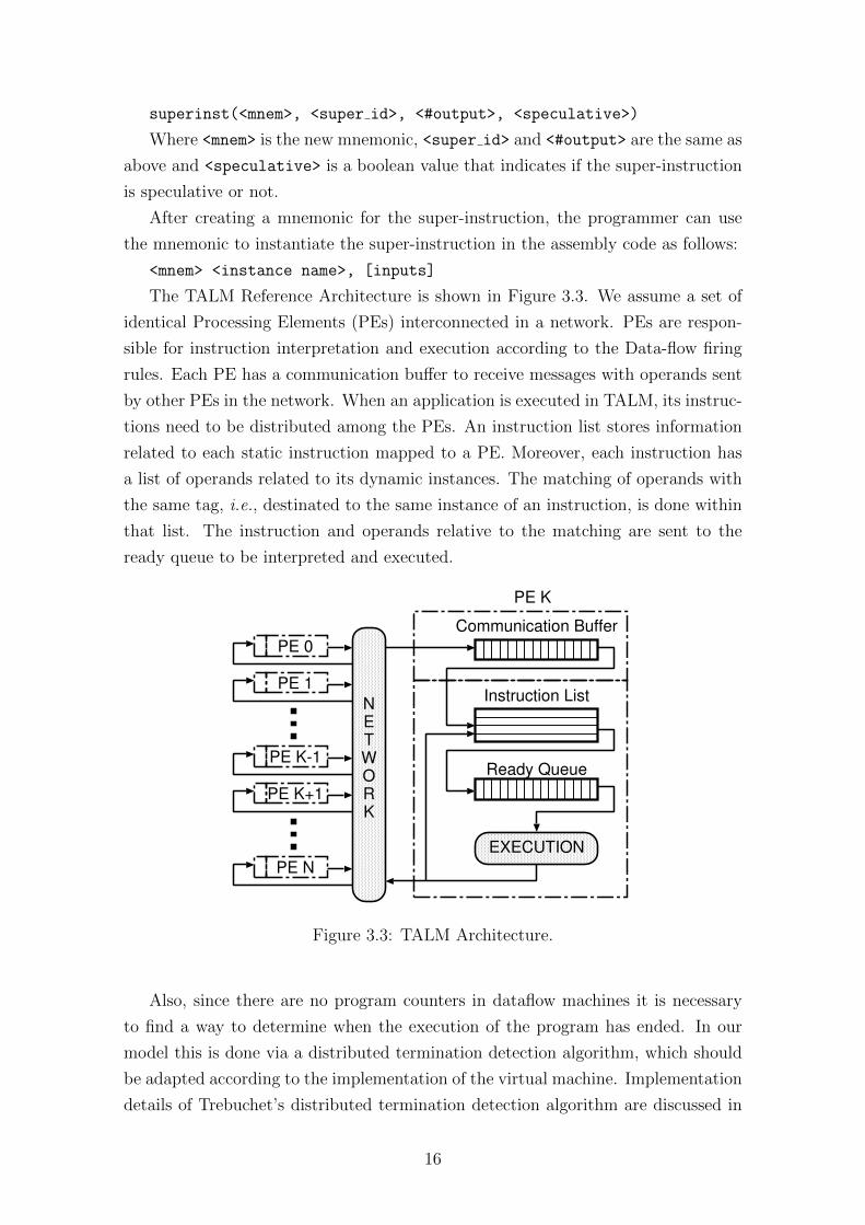
The TALM Reference Architecture is shown in Figure 3.3. We assume a set of

identical Processing Elements (PEs) interconnected in a network. PEs are respon-

sible for instruction interpretation and execution according to the Data-flow firing

rules. Each PE has a communication buffer to receive messages with operands sent

by other PEs in the network. When an application is executed in TALM, its instruc-

tions need to be distributed among the PEs. An instruction list stores information

related to each static instruction mapped to a PE. Moreover, each instruction has

a list of operands related to its dynamic instances. The matching of operands with

the same tag, i.e., destinated to the same instance of an instruction, is done within

that list. The instruction and operands relative to the matching are sent to the

ready queue to be interpreted and executed.

EXECUTION

PE 0

PE K

NETWORK

Communication Buffer

Instruction List

Ready Queue

PE 1

PE K-1

PE K+1

PE N

Figure 3.3: TALM Architecture.

Also, since there are no program counters in dataflow machines it is necessary

to find a way to determine when the execution of the program has ended. In our

model this is done via a distributed termination detection algorithm, which should

be adapted according to the implementation of the virtual machine. Implementation

details of Trebuchet’s distributed termination detection algorithm are discussed in

16

depth in Section 3.3.3.

3.3 Trebuchet: TALM for multicores

Trebuchet is an implementation of TALM for multi-core machines. In this section

we discuss the main implementation issues and describe how we use Trebuchet to

parallelise programs.

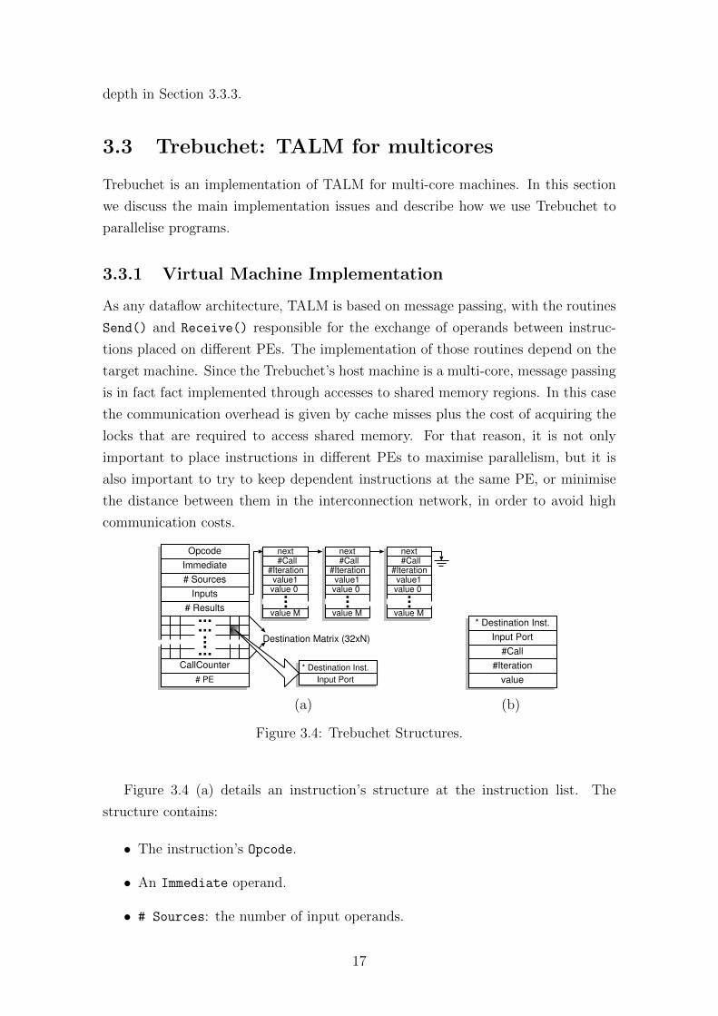
3.3.1 Virtual Machine Implementation

As any dataflow architecture, TALM is based on message passing, with the routines

Send() and Receive() responsible for the exchange of operands between instruc-

tions placed on different PEs. The implementation of those routines depend on the

target machine. Since the Trebuchet’s host machine is a multi-core, message passing

is in fact fact implemented through accesses to shared memory regions. In this case

the communication overhead is given by cache misses plus the cost of acquiring the

locks that are required to access shared memory. For that reason, it is not only

important to place instructions in different PEs to maximise parallelism, but it is

also important to try to keep dependent instructions at the same PE, or minimise

the distance between them in the interconnection network, in order to avoid high

communication costs.

Opcode

Immediate

Inputs

# Sources

# Results

CallCounter

# PE

Destination Matrix (32xN)

* Destination Inst.

Input Port

value 0value1

value M

next#Call

#Iteration

value 0value1

value M

next#Call

#Iteration

value 0value1

value M

next#Call

#Iteration

* Destination Inst.

Input Port

#Call

#Iteration

value

(a) (b)

Figure 3.4: Trebuchet Structures.

Figure 3.4 (a) details an instruction’s structure at the instruction list. The

structure contains:

• The instruction’s Opcode.

• An Immediate operand.

• # Sources: the number of input operands.

17

• Inputs: a linked list to store matching structures. Each element contains a

pointer to the next element in the list, the tag (#Call and #Iteration) and

up to 32 operands. A match will occur when all operands (# Sources) are

present.

• # Results: the number of output operands produced by a certain instruction.

• The Destination Matrix, that indicates where to send the operands that are

produced by a certain instruction. Each line specifies N destinations for an

operand. Each element of this matrix contains a pointer to the destination

instruction and the number of the input port (Port) in which the operand will

be inserted when it reaches its destination.

• The CallCounter field is used by the callsnd instruction to store the value

of the call counter, mentioned in Section 3.1. In this case, the Immediate field

is used to store CallGrp, explained in the same section.

• # PE: each instruction has the number of the PE to which it is mapped. Notice

that operands exchanged between instructions placed in the same PE will not

be sent through the network. Instead, they will be directly forwarded to their

destination instruction in the list.

Figure 3.4 (b) shows a message with a single operand, to be exchanged between

PEs. The message contains a pointer to the destination instruction, the destination

input port number, and the operand itself.

3.3.2 Parallelising Applications with Trebuchet

To parallelise sequential programs using Trebuchet it is necessary to compile them

to TALM’s Data-flow assembly language and run them on Trebuchet. Trebuchet is

implemented as a virtual machine and each of its PEs is associated with a thread

at the host machine. When a program is executed on Trebuchet, instructions are

allocated to the PEs and fired according to the Data-flow model. Independent

instructions will run in parallel if they are mapped to different PEs and there are

available cores at the host machine to run those PEs’ threads simultaneously.

Since interpretation costs can be high, the execution of programs fully com-

piled to Data-flow might present unsatisfactory performance. To address this prob-

lem, blocks of Von Neumann code are transformed into super-instructions. Those

blocks are compiled to the host machine as usual and the interpretation of a super-

instruction will come down to simple call to the direct execution of the related

block. Notice that the execution of each super-instruction is still fired by the virtual

machine, according to the Data-flow model. This is one of the main contributions

18

introduced by Trebuchet: allowing the definition of Von Neumann blocks with dif-

ferent granularity (not only methods as in Program Demultiplexing), besides not

demanding hardware support.

Data-flow Assembly

.fl

C Source

.c

Data-flowAssembly process

LibraryCompilation

Library binary

.df.so

Data-flow AssemblyManual Coding

DataFlow binary

.flb

Placement

EP N

Blocks Definition /Source Transformation

Transformed Source

.df.c

EP 2inst 32inst 45inst 60

EP 1inst 3inst 50inst 52

inst 19inst 39inst 43

BinaryLoad

Execution

Figure 3.5: Work-flow to follow when parallelising applications with Trebuchet.

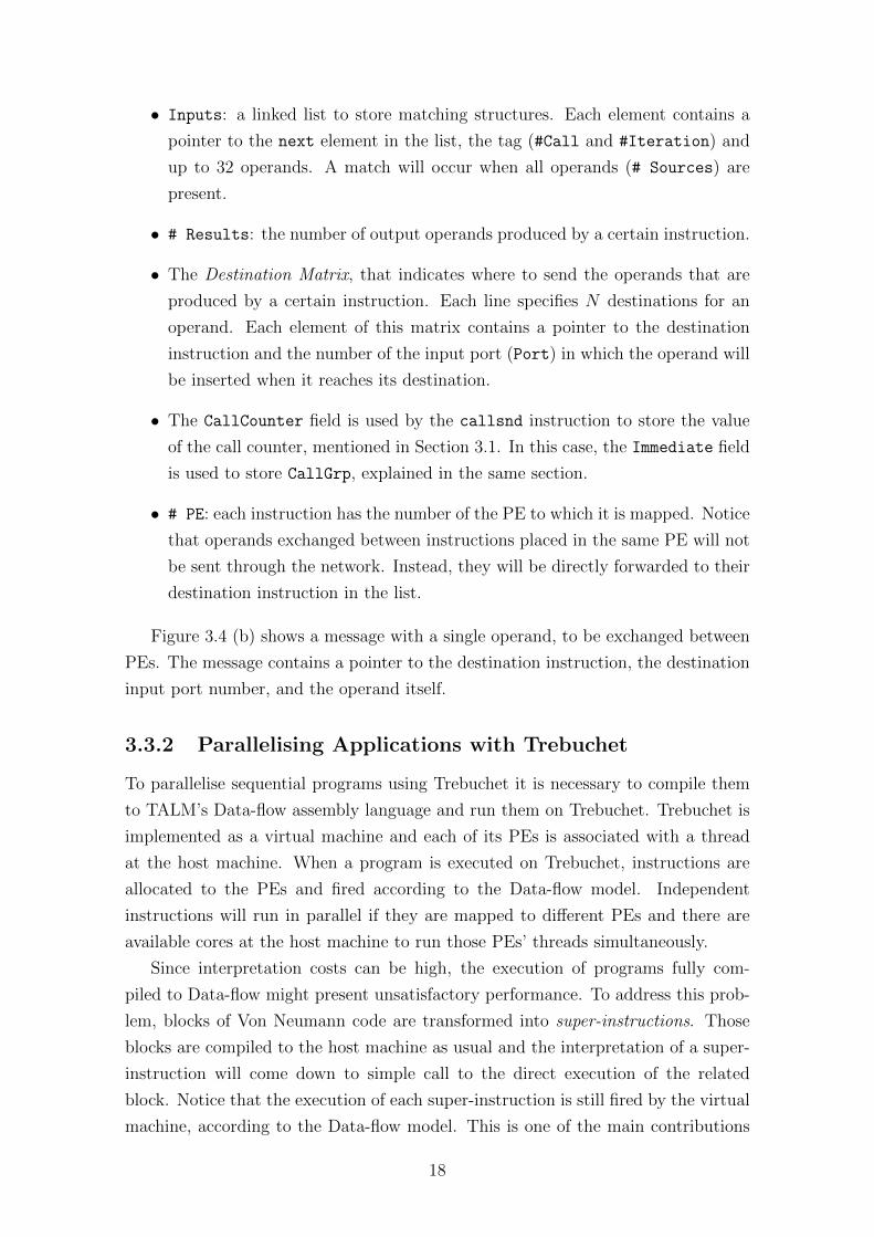
Figure 3.5 shows the work-flow to be followed in order to parallelise a sequen-

tial program and execute it in Trebuchet. Initially, blocks that will form super-

instructions are defined through a code transformation. The code transformation

ensures that the block can be addressed separately and marks the entry points. Pro-

filing tools may be used in helping to determine which portions of code are interesting

candidates to parallelisation. The transformed blocks are then compiled into a dy-

namic library, that will be available to the abstract machine interpreter. Then, a

dataflow graph connecting all blocks is defined and the dataflow assembly code is

generated. The code may have both super-instructions and simple (fine-grained)

instructions. Next, a dataflow binary is generated from the assembly, processor

placement is defined, and the binary code is loaded and executed. Execution of sim-

ple instructions requires full interpretation, whereas super-instructions are directly

executed on the host machine.

We have implemented an assembler for TALM and a loader for Trebuchet, in

order to automatise the dataflow binary code generation and program loading. The

definition of super-instructions and instructions placement, are performed manually

in our current implementation. Besides, we still do not have a dataflow compiler

for Trebuchet. This means that the fragments of the original C code that were

19

not selected to be part of super-instructions will have to be translated manually

to Trebuchet’s assembly language. We consider that this tools are necessary and

developing them is part of ongoing work.

+ ++

* result

const nT, 4const tID0, 0const tID1, 1const tID2, 2const tID3, 3const n, 10000fconst h, 0.00001

pI0 pI1 pI2 pI3

fadd r0, pI0.0, pI1.0fadd r1, pI2.0, pI3.0fadd r2, r0, r1fmul result, r2, h

superinst ("pI", 0, 1)pI pI0, nT, tID0, h, npI pI1, nT, tID1, h, npI pI2, nT, tID2, h, npI pI3, nT, tID3, h, n 00101010010

0101101001110010011110100101111111110101000000010100101

IN.df.so(binary)

void main() { int i, n = 10000; float h = 0.00001; float sum = 0; for (i=0; i<n; i++) sum += f((i-0.5)*h); sum *= h;}

IN.cvoid super0(oper_t **oper, oper_t *result){ int nT = oper[0]->value.i; int tID = oper[1]->value.i; int i, n = oper[3]->value.i; float h = oper[2]->value.i; float sum = 0; for (i=tID; i<n; i+=nT) sum += f((i-0.5)*h); result[0].value.f = sum;}

IN.df.cA

B

C

D E

Const #4

nh

tID1tID0 tID2 tID3

Initialization

Partial summations

Result

Figure 3.6: Using Trebuchet.

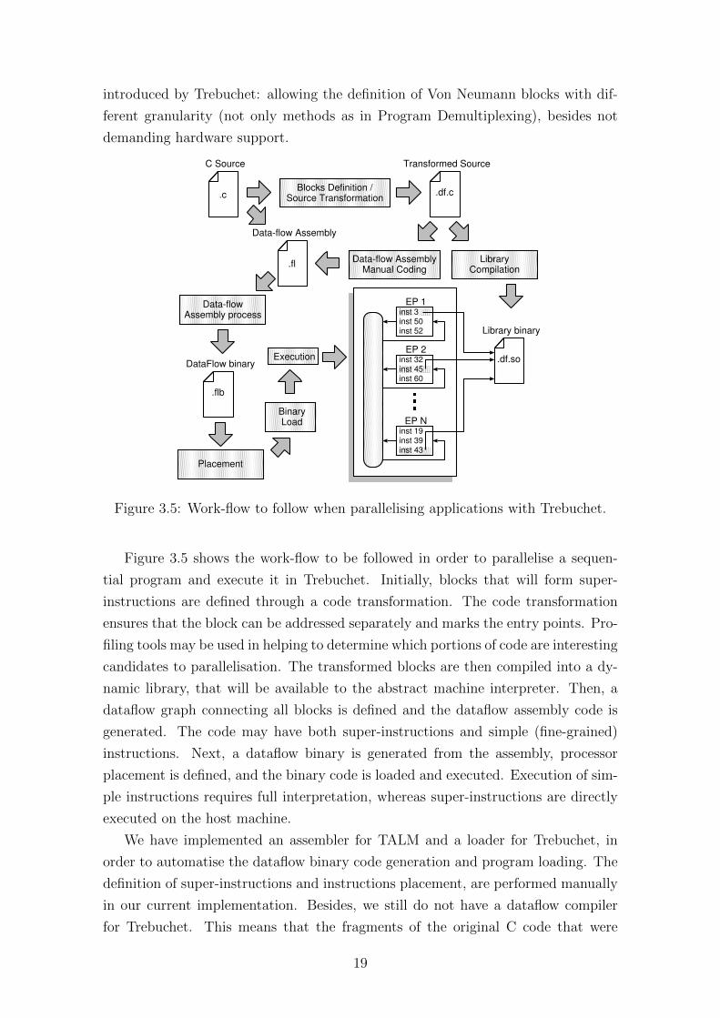
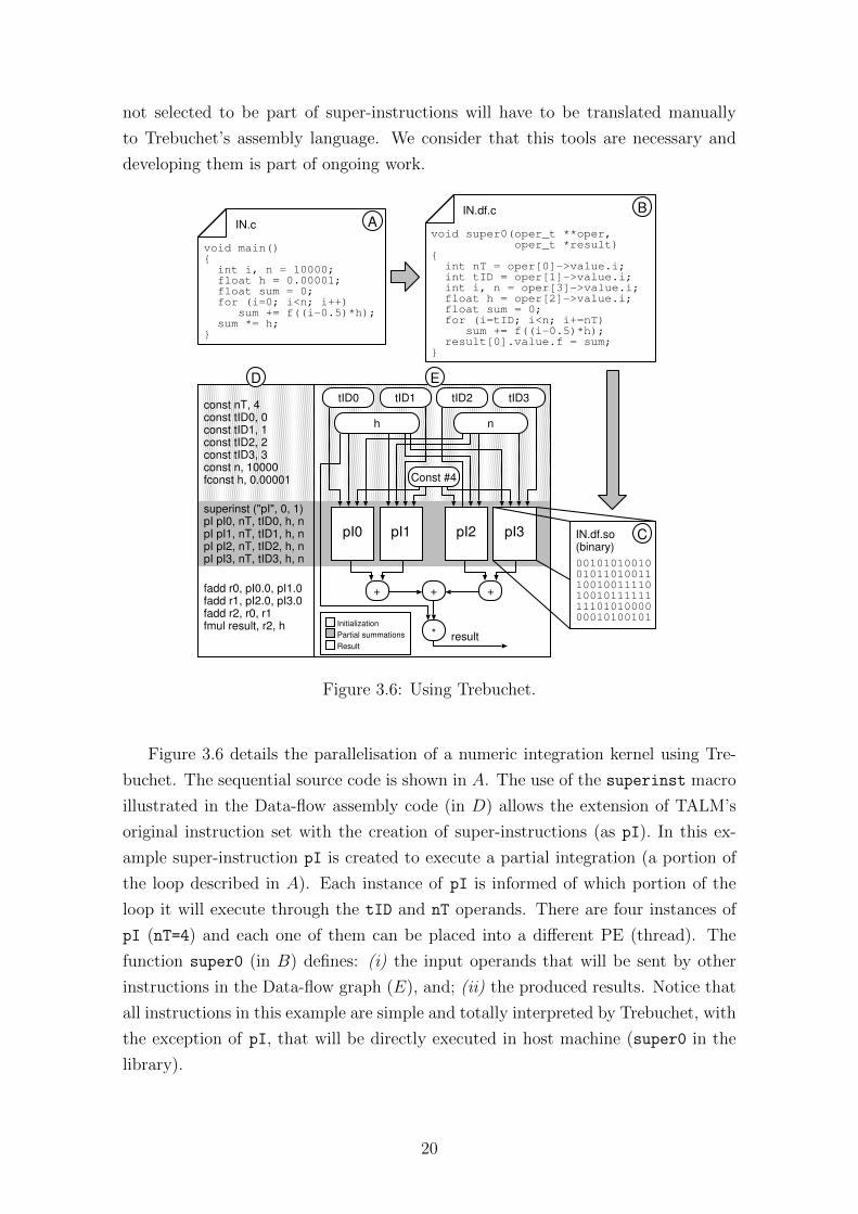
Figure 3.6 details the parallelisation of a numeric integration kernel using Tre-

buchet. The sequential source code is shown in A. The use of the superinst macro

illustrated in the Data-flow assembly code (in D) allows the extension of TALM’s

original instruction set with the creation of super-instructions (as pI). In this ex-

ample super-instruction pI is created to execute a partial integration (a portion of

the loop described in A). Each instance of pI is informed of which portion of the

loop it will execute through the tID and nT operands. There are four instances of

pI (nT=4) and each one of them can be placed into a different PE (thread). The

function super0 (in B) defines: (i) the input operands that will be sent by other

instructions in the Data-flow graph (E), and; (ii) the produced results. Notice that

all instructions in this example are simple and totally interpreted by Trebuchet, with

the exception of pI, that will be directly executed in host machine (super0 in the

library).

20

3.3.3 Global termination detection

In the Von Neumann model, the end of execution is identified when the program

counter reaches the end of the code. In the case of a machine with multiple Von

Neumann cores, this condition is generalised to when all the program counters reach

the end of their respective core’s code. On Data-flow machines this property of the

execution status cannot be inferred as easily because the processing elements only

have information about their local state. When a processing element finds itself idle,

i.e., with its ready queue empty, it cannot assume the entire program has ended

because other PEs might still be working or there might be operands traveling

through the system that will trigger new instruction executions on it. Hence, a

way of knowing the state of the whole system, PEs and communication edges, is

needed. For this purpose, a customised implementation of the Distributed Snapshots

Algorithm [22] was employed. The algorithm detects a state where all PEs are idle

and all communication edges are empty, meaning that the program has terminated

its execution because no more work will be done.

There are two main differences between our specialised implementation and the

generic form of the algorithm: since our topology is a complete graph we don’t need

a leader (each node can gather all the information it needs from the others by itself)

and since we only need to detect if the program has terminated or not we only use

one kind of message, the termination marker.

A node (PE) begins a new termination detection after entering state (isidle = 1),

which means it has no instructions in its ready queue. It then broadcasts a marker

with a termination tag equal to the greatest marker tag seen plus 1. Other nodes

enter that termination detection if they already are in state (isidle = 1) and if the

tag received is greater than the greatest termination tag seen so far. After entering

the new termination detection the other nodes also broadcast the marker received,

indicating to all their neighbors that they are in state (isidle = 1).

Once a node participating in a termination detection has received a marker

corresponding to that run of the algorithm from all its neighbors, i.e., all other

nodes, in the complete graph topology, it broadcasts another marker with the same

termination tag if it is still in state (isidle = 1). The second marker broadcast

carries the information that all input edges of that node were detected empty, since

the node only broadcasted the marker because it stayed in state (isidle = 1) until

receiving the first round of markers from all other nodes, meaning it did not receive

a message containing an operand.

So, in our implementation only one type of message is used: the marker with

the termination tag. The first round of markers carries the information of the node

states (isidle = 1), while the second round carries the input edges state information

21

(all empty). It is then clear that after receiving the second round of markers from

all neighbors, the node can terminate.

3.4 Describing Pipelines in TALM

Pipelining is a parallel programming pattern in which one operation is divided into

different stages. Although there are dependencies between stages, since data is

forwarded between stages, there is parallelism available since stages can operate

on different sets of data concurrently. The dataflow model allows us to describe

pipelines in a straightforward manner, just by describing the dependencies between

stages, without needing to implement any further synchronization.

Suppose we have a video streaming server, which reads data for each video frame,

compresses it and then sends the compressed data to the client. This server could

be implemented as a pipeline, since its operation could be split into three stages

(read, compress and send) and the stag es could execute in parallel, each working

on a different frame.

To describe a pipeline in TALM, we simply implement the stages as super-

instructions and connect them in the dataflow graph corresponding to the pipeline.

In Figure 3.7 we describe a complete example of how a pipeline with complex de-

pedencies can be implemented in TALM. Pane A shows the sequential code for the

kernel in C language, pane B has the stages implemented as super-instructions and

in pane C we have the dataflow graph that describe the dependencies.

To compute this kernel, the values of X depend on the values of K from the

previous iteration. The values of K, on the other hand, depend on the values of

X from the same iteration and the values of X from the same iteration and the

values of N depend just on the values of K from the same iteration. Besides those

dependencies, the value of the variable stay, used as the loop control, depends on

the computation of the values of K. This way the super-instruction s0, responsable

for calculating X, can star executing the next execution as soon as s1 finishes the

current iteration, since there is no need to wait for s2 to finish.

The flexibility to describe this kind of pipeline is a strong point of TALM in

comparison with other models. It is not possible to describe such complex pipelines

using Intel Threading Building Blocks [9, 23] pipeline template, since it only allows

linear pipelines.

3.5 THLL (TALM High Level Language)

Describing a datafow graph directly in TALM assembly language can be an ardous

and complex task as the number of instructions grows. Besides the graphs described

22

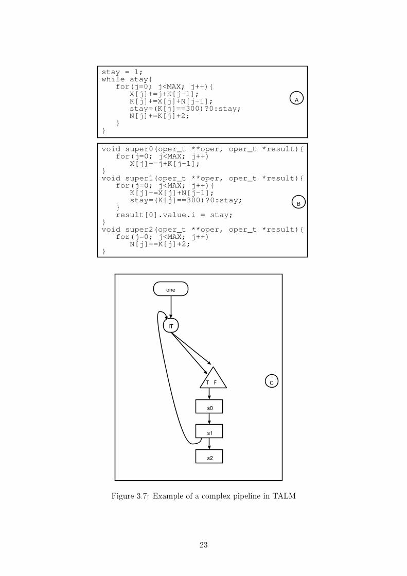
stay = 1;while stay{ for(j=0; j<MAX; j++){ X[j]+=j+K[j-1]; K[j]+=X[j]+N[j-1]; stay=(K[j]==300)?0:stay; N[j]+=K[j]+2; }}

void super0(oper_t **oper, oper_t *result){ for(j=0; j<MAX; j++) X[j]+=j+K[j-1]; }void super1(oper_t **oper, oper_t *result){ for(j=0; j<MAX; j++){ K[j]+=X[j]+N[j-1]; stay=(K[j]==300)?0:stay; } result[0].value.i = stay;}void super2(oper_t **oper, oper_t *result){ for(j=0; j<MAX; j++) N[j]+=K[j]+2;}

A

B

IT

T F

one

s1

s2

s0

C

Figure 3.7: Example of a complex pipeline in TALM

23

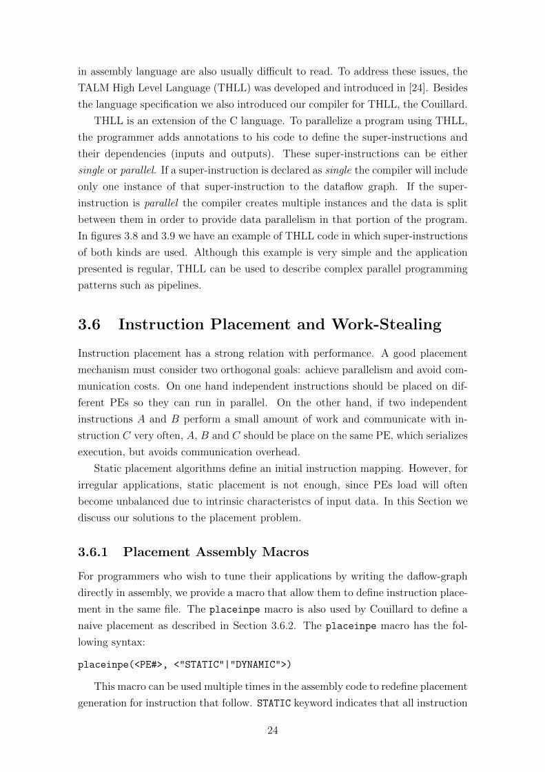
in assembly language are also usually difficult to read. To address these issues, the

TALM High Level Language (THLL) was developed and introduced in [24]. Besides

the language specification we also introduced our compiler for THLL, the Couillard.

THLL is an extension of the C language. To parallelize a program using THLL,

the programmer adds annotations to his code to define the super-instructions and

their dependencies (inputs and outputs). These super-instructions can be either

single or parallel. If a super-instruction is declared as single the compiler will include

only one instance of that super-instruction to the dataflow graph. If the super-

instruction is parallel the compiler creates multiple instances and the data is split

between them in order to provide data parallelism in that portion of the program.

In figures 3.8 and 3.9 we have an example of THLL code in which super-instructions

of both kinds are used. Although this example is very simple and the application

presented is regular, THLL can be used to describe complex parallel programming

patterns such as pipelines.

3.6 Instruction Placement and Work-Stealing

Instruction placement has a strong relation with performance. A good placement

mechanism must consider two orthogonal goals: achieve parallelism and avoid com-

munication costs. On one hand independent instructions should be placed on dif-

ferent PEs so they can run in parallel. On the other hand, if two independent

instructions A and B perform a small amount of work and communicate with in-

struction C very often, A, B and C should be place on the same PE, which serializes

execution, but avoids communication overhead.

Static placement algorithms define an initial instruction mapping. However, for

irregular applications, static placement is not enough, since PEs load will often

become unbalanced due to intrinsic characteristcs of input data. In this Section we

discuss our solutions to the placement problem.

3.6.1 Placement Assembly Macros

For programmers who wish to tune their applications by writing the daflow-graph

directly in assembly, we provide a macro that allow them to define instruction place-

ment in the same file. The placeinpe macro is also used by Couillard to define a

naive placement as described in Section 3.6.2. The placeinpe macro has the fol-

lowing syntax:

placeinpe(<PE#>, <"STATIC"|"DYNAMIC">)

This macro can be used multiple times in the assembly code to redefine placement

generation for instruction that follow. STATIC keyword indicates that all instruction

24

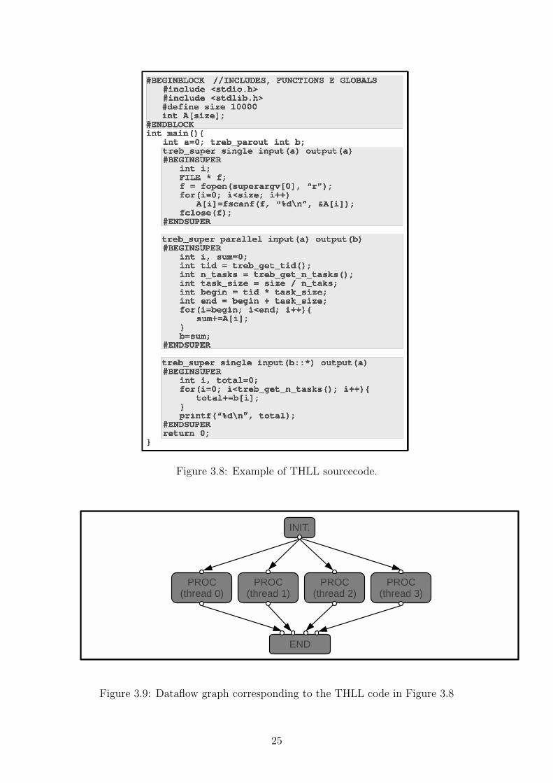
Figure 3.8: Example of THLL sourcecode.

Figure 3.9: Dataflow graph corresponding to the THLL code in Figure 3.8

25

that follow must be mapped to the same PE (indicated by PE#). DYNAMIC keyword

indicates that each time a parallel super-instruction (or instruction) is found, each

of its instances will be mapped to diffent PEs, starting by PE#.

3.6.2 Couillard Naive Placement

For applications that are ballanced and follow a simple parallelism pattern a naive

placement algorith should usually be enough. Regular applications that follow the

fork/join pattern, for example, should only have their parallel super-instructions

equaly distributed among PEs to achieve maximum parallelism and this would usu-

ally suffice.

This strategy is the one adopted by Couillard. It basically generates assembly

code that uses palceinpe(0,"DYNAMIC") for all parallel super-instructions.

3.6.3 Static Placement Algorithm

3.7 Static Scheduling

Since our model relies on both static and dynamic scheduling of the instructions, we

needed to develop strategies for static scheduling (as work-stealing is our dynamic

scheduling mechanism). The algorithm we adopted for mapping instructions to PEs

in compile time is a variation of previous list scheduling algorithms with dynamic

priorities ([14–16]).

The most significant improvement introduced to the traditional list scheduling

techniques present in our algorithm is the adoption of the probabilities associated

with conditional edges of the graph as a priority level for the instruction mapping.

In a similar fashion to the execution models presented in [25], our dataflow graphs

have conditional edges (the ones that come out of steer instructions) which will only

forward data through them if the boolean operand sent to the steer instruction is

true, in case of the first output port, or false, in case of the second output port.

Traditionally, list scheduling algorithms try to map instructions that have depen-

dencies close to each other. Since an input operand can come from multiple source

instructions, due to conditional edges, real dependencies are only known during ex-

ecution. Due to this, our algorithm uses the probabilities associated with the edges

(i.e. the probability that a certain edge will forward data) to prioritize dependencies

that are more likely to really occur during execution.

The probabilities of the edges in the dataflow graph D = (I, E) are computed in

the first step of our algorithm. Each each e ∈ E has a probability φ(e) associated

with it, which is a boolean function of variables used to control steer instructions

in the graph. First, it is necessary to estimate the probability that each boolean

26

variable in the graph is true. This must be done in the same way as branch prediction

hints are used in architectures that adopt them. A profiling of executions of the

dataflow graph must be done to come up with an estimation of the percentage of

times that the variable is forwarded as true. Based on this statistical profiling of

control variables it becomes possible to define the edge probabilities in a recursive

manner. First we shall introduce the notation we use:

• (ap, bq) represents an edge between the output port p of instruction a and the

input port q of instruction b. The the input/output may be omitted if the

context does not require their specification.

• bool(e) is the control variable forwared through edge e.

• B(e) = P (bool(e) = True) is the probability of bool(e) being True, which

is estimated via profiling of executions of the dataflow graph. Conversely,

¬B(e) = (1−B(e)).

• inports(i) the set of input ports of instruction i

• outports(i) the set of output ports of instruction i.

Now, given a dataflow graph D = (I, E) where I is the set of instructions and

E the set of edges connection them, we can define the probability φ(e) of each edge

e = (a, b) ∈ E as the following:

• 1, if a is a root (i.e. there is no i ∈ I such that (i, a) ∈ E).

•∑{φ(e) · B(e) | e = (·, a0) ∈ E}, if a is a steer and e comes from output port

0 of a (i.e. the True port)

•∑{φ(e) · ¬B(e) | e = (·, a0) ∈ E}, if a is a steer and e comes from output port

1 of a (i.e. the False port)

•∏

p∈inports(a)

(∑{φ(e) | e = (·, ap) ∈ E}), otherwise.

It is also necessary to define the rest of the parameters we use in our algorithm.

P is the set of processing elements available. In our current implementation, all PEs

are equal so the average execution time of instructions do not vary depending on

which PE the are executed. Hence, we just express the average execution time of

instruction i as ti.

The average time it takes to send the data corresponding to one operand from PE

to another is also considered homogeneous, since the current implementation uses

shared memory. In case the data that one instruction produces and is consumed by

27

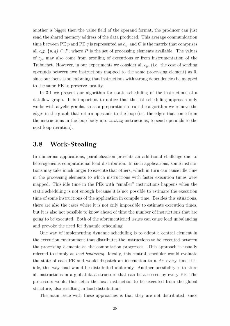
another is bigger then the value field of the operand format, the producer can just

send the shared memory address of the data produced. This average communication

time between PE p and PE q is represented as cqp and C is the matrix that comprises

all cqp, {p, q} ⊆ P , where P is the set of processing elements available. The values

of cpq may also come from profiling of executions or from instrumentation of the

Trebuchet. However, in our experiments we consider all cpp (i.e. the cost of sending

operands between two instructions mapped to the same processing element) as 0,

since our focus is on enforcing that instructions with strong dependencies be mapped

to the same PE to preserve locality.

In 3.1 we present our algorithm for static scheduling of the instructions of a

dataflow graph. It is important to notice that the list scheduling approach only

works with acyclic graphs, so as a preparation to run the algorithm we remove the

edges in the graph that return operands to the loop (i.e. the edges that come from

the instructions in the loop body into inctag instructions, to send operands to the

next loop iteration).

3.8 Work-Stealing

In numerous applications, parallelization presents an additional challenge due to

heterogeneous computational load distribution. In such applications, some instruc-

tions may take much longer to execute that others, which in turn can cause idle time

in the processing elements to which instructions with faster execution times were

mapped. This idle time in the PEs with “smaller” instructions happens when the

static scheduling is not enough because it is not possible to estimate the execution

time of some instructions of the application in compile time. Besides this situations,

there are also the cases where it is not only impossible to estimate execution times,

but it is also not possible to know ahead of time the number of instructions that are

going to be executed. Both of the aforementioned issues can cause load unbalancing

and provoke the need for dynamic scheduling.

One way of implementing dynamic scheduling is to adopt a central element in

the execution environment that distributes the instructions to be executed between

the processing elements as the computation progresses. This approach is usually

referred to simply as load balancing. Ideally, this central scheduler would evaluate

the state of each PE and would dispatch an instruction to a PE every time it is

idle, this way load would be distributed uniformly. Another possibility is to store

all instructions in a global data structure that can be accessed by every PE. The

processors would thus fetch the next instruction to be executed from the global

structure, also resulting in load distribution.

The main issue with these approaches is that they are not distributed, since

28

Algorithm 3.1 Algorithm for scheduling dataflow graphs

Input: Dataflow graph D = (I, E), the set of processing elements P , the interpro-cessor communication costs matrix C and the average execution time ti of eachinstruction.

Output: A mapping of I → PCalculate the priorities of all instructions and the probability φ(e) associated witheach edge e ∈ Eready ← All i ∈ I such that {j|(j, i) ∈ E} = ∅Initialize all makespan(p), p ∈ P with 0while ready 6= ∅ do

Remove the instruction i with the highest priority from ready.MAP(i)Mark all edges (i, ·) going out of iAdd to ready the instructions that have become ready after this (i.e. all input

edges have been marked).end whileprocedure map(i)

finish(i)←∞for all p ∈ P do

Pick edge e = (j, i) ∈ E such that (finish(j) + cqp) ·φ(e) is the maximum,where j was mapped to processor q

aux← max(finish(j) + cqp,makespan(p)) + tiif aux < finish(i) then

finish(i)← auxchosenproc← p

end ifend formap i to chosenprocmakespan(p)← finish(i)

end procedure

29

there is a need for either a central agent or a global data structure shared by all

processing elements. Besides that, it is also not possible to use static scheduling,

since all the mapping of instructions would be time in execution time.

One approach for dynamic scheduling that does not incur in these shortcomings

is work-stealing. In a system with work-stealing, instructions are mapped normally

at compile time with some static scheduling algorithm and then, during execution,

PEs that find themselves idle (due to unbalance) access their neighbors’ data struc-

tures to fetch instructions that are ready to execute. Observe that, in the case

where the computanional load is homogeneous and is uniformly distributed by the

static scheduling, the work-stealing will simply not be used. Therefore, one great

advantage of work-stealing over the other dynamic scheduling approaches is that

accesses to concurrent data structures only occur when there is unbalance in the

load distribution.

In Section 2.3 we mentioned some of the most influential prior work on work-

stealing. Most of the work-stealing algorithms adopt deques (double ended queues)

to store instructions that are ready to execute. In these algorithms, each thread

has its own deque, but if it becomes idle, i.e. its deque becomes empty, the thread

may try to steal work from the deques of neighbors. As the name indicates, deques

are queues that may be acessed by both ends, namely the owner of the deque will

pop instructions from one end and the thieves will steal instructions from the other

end. This way the thieves have less influence in the accesses made by the owner of

the deque, since owners and thieves do not usually compete to access the deque as

they are accessing different ends of it. Actually, the only time the deque owner will

have to compete with a thief is if they are both trying to pop the last instruction

remaining in the deque.

This strategy, however, forces thieves to always try to steal the instruction that

is on the end of deque, not giving them the option to choose. In some situations

this might be suboptimal, since it might be desirable to choose which instruction to

steal. For instance, consider a heterogeous system, where instructions have different

average execution times on each PE. In this case, a thief would want to steal the

instructions that run the fastest on it, disregarding the ones that are slow on that

PE. The same reasoning can be made about cache locality, it might be wise to

choose instructions that will take advantage of data locality on that PE and avoid

cache pollution. Yet another, more intuitive, reason why to choose what instructions

to steal is that in order to maximize efficiency it is preferable to steal instructions

that are more coarse-grained, since that will increase the useful computation per

overhead ratio.

For these reasons we developed in this work the Selective Work Stealing (SWS)

algorithm. Using SWS it is possible for a thief PE to navigate through a victim’s

30

deque in order to search for an instruction that, according to some heuristic, is a good

fit for work-stealing. In Section 3.8.1 we will present the algorithm for SWS. As per

convention and to maintain compatibility with the rest of work-stealing bibilography,

we will use the term “tasks” to refer to the execution unit that is stolen, but keep

in mind that in the scope of this work we are talking about dataflow instructions.

3.8.1 Selective Work-Stealing

The Selective Work-Stealing Algorithm (SWS) is based on the algorithm preseted

by Arora et al. in [17]. SWS also uses deques (double ended queues) to store the

ready tasks, but our implementation differs from the one presented in [17] because

we add new functionalities in order to support selective work-stealing.

A deque is a structure similar to a FIFO queue, but, as opposed to traditional

queues, in a deque elements can be included from or added to both ends of the

structure. In work-stealing algorithms the owner thread pops tasks from one end

of the deque and the thieves steal tasks from the other end, thus reducing the

interference of thieves in the owner thread’s performance. In general, the owner

thread both inserts and removes tasks from the same size of the deque. This way,

for the owner thread the deque has LIFO (last in first out) policy for the owner

thread and FIFO (first in first out) policy for the thieves. This set of policies is

adequate for recursive applications (search algorithms, for example) mas it is not

the best behaviour for most of the applications we study in our work. Since the

computations with which we experiment are mainly comprised by loops, we want

the owner thread to remove tasks from de deque in a FIFO, since in order to trigger

the execution of new loop iterations you may have to first finish executing pending

iterations. For that reason we chose to invert the access policies in our algorithm.

In order to allow a thread to select which task it wants to steal, it was necessary to

add the necessary logic to the algorithm to allow tasks to be stolen from the middle

of the deque, not just from one end. A simple and direct way to implement a deque

with that functionality would be using concurrent linked lists, but the performance

would not be very good due to the indirect memory accesses inherent to linked lists

and to the complexity of developing synchronization to allow a linked list to be

accessed concurrently. Hence our choice of keeping the deque implemented as an

array, but having the thief threads access it in a fashion similar to linked lists.

Figure 3.10 introduces de deque structure used in the algorithm. The deque is

comprised by an array of tasks, one anchor for the deque owner and chained anchors

for each thief. The access to the array is done in a circular fashion, i.e. the memory

address of the position k in the array is calculate in the operation b + (k mod l),

where b is the address of the buffer allocated for the array and l is the number of

31

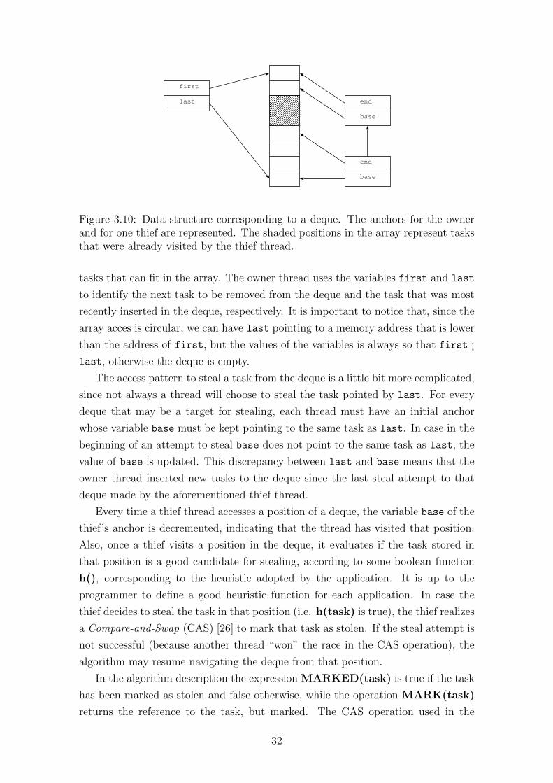
first

last

base

end

base

end

Figure 3.10: Data structure corresponding to a deque. The anchors for the ownerand for one thief are represented. The shaded positions in the array represent tasksthat were already visited by the thief thread.

tasks that can fit in the array. The owner thread uses the variables first and last

to identify the next task to be removed from the deque and the task that was most

recently inserted in the deque, respectively. It is important to notice that, since the

array acces is circular, we can have last pointing to a memory address that is lower

than the address of first, but the values of the variables is always so that first ¡

last, otherwise the deque is empty.

The access pattern to steal a task from the deque is a little bit more complicated,

since not always a thread will choose to steal the task pointed by last. For every

deque that may be a target for stealing, each thread must have an initial anchor

whose variable base must be kept pointing to the same task as last. In case in the

beginning of an attempt to steal base does not point to the same task as last, the

value of base is updated. This discrepancy between last and base means that the

owner thread inserted new tasks to the deque since the last steal attempt to that

deque made by the aforementioned thief thread.

Every time a thief thread accesses a position of a deque, the variable base of the

thief’s anchor is decremented, indicating that the thread has visited that position.

Also, once a thief visits a position in the deque, it evaluates if the task stored in

that position is a good candidate for stealing, according to some boolean function

h(), corresponding to the heuristic adopted by the application. It is up to the

programmer to define a good heuristic function for each application. In case the

thief decides to steal the task in that position (i.e. h(task) is true), the thief realizes

a Compare-and-Swap (CAS) [26] to mark that task as stolen. If the steal attempt is

not successful (because another thread “won” the race in the CAS operation), the

algorithm may resume navigating the deque from that position.

In the algorithm description the expression MARKED(task) is true if the task

has been marked as stolen and false otherwise, while the operation MARK(task)

returns the reference to the task, but marked. The CAS operation used in the

32

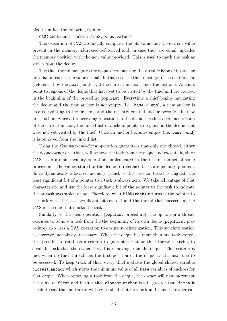
algorithm has the following syntax:

CAS(<address>, <old value>, <new value>)

The execution of CAS atomically compares the old value and the current value

present in the memory addressed referenced and, in case they are equal, uptades

the memory position with the new value provided. This is used to mark the task as

stolen from the deque.

The thief thread navigates the deque decrementing the variable base of its anchor

until base reaches the value of end. In this case the thief must go to the next anchor

(referenced by the next pointer), if the current anchor is not the last one. Anchors

point to regions of the deque that have yet to be visited by the thief and are created

in the beginning of the procedure pop last. Everytime a thief begins navigating

the deque and the first anchor is not empty (i.e. base ≥ end), a new anchor is

created pointing to the first one and the recently created anchor becomes the new

first anchor. Since after accessing a position in the deque the thief decrements base

of the current anchor, the linked list of anchors points to regions in the deque that

were not yet visited by the thief. Once an anchor becomes empty (i.e. base ¡ end)

it is removed from the linked list.

Using the Compare-and-Swap operation guarantees that only one thread, either

the deque owner or a thief, will remove the task from the deque and execute it, since

CAS is an atomic memory operation implemented in the instruction set of some

processors. The values stored in the deque to reference tasks are memory pointers.

Since dynamically allocated memory (which is the case for tasks) is aligned, the

least significant bit of a pointer to a task is always zero. We take advantage of that

characteristic and use the least significant bit of the pointer to the task to indicate

if that task was stolen or no. Therefore, what MARK(task) returns is the pointer to

the task with the least significant bit set to 1 and the thread that succeeds at the

CAS is the one that marks the task.

Similarly to the steal operation (pop last procedure), the operation a thread

executes to remove a task from the the beginning of its own deque (pop first pro-

cedure) also uses a CAS operation to ensure synchronization. This synchronization

is, however, not always necessary. When the deque has more than one task stored,

it is possible to establish a criteria to guarantee that no thief thread is trying to

steal the task that the owner thread is removing from the deque. This criteria is

met when no thief thread has the first position of the deque as the next one to

be accessed. To keep track of that, every thief updates the global shared variable

closest anchor which stores the minimum value of all base variables of anchors for

that deque. When removing a task from the deque, the owner will first increment

the value of first and if after that closest anchor is still greater than first it

is safe to say that no thread will try to steal that first task and thus the owner can

33

just remove the task without the need for a CAS operation. This is one of the great

advantages of this kind of algorithm, it lessens the overheads on the deque owner.

In order to add a new task to the deque the owner first includes the task in

the position after the one that is currently the last and subsequently updated the

last variable of the deque. Notice that the order in which these two operations are

performed is vital to the correctness of the algorithm. If last is updated before

the task is actually added to the deque, a thief may read data from the deque

that is not a reference for a valid task. In some processors the order of the two

operations (storing the new task in the array and writing the variable) may not be

guaranteed. This occurs because the memory system of these processors considers it

safe to reorder memory operations that target different memory addresses and have

no data dependencies between them. Although such reordering would be fine in

sequential execution, it can be harmful in a parallel program. To avoid this kind of

problem it is necessary to use some kind of store barrier, like the lfence instruction

of x86 instruction sets, to guarantee that the variable write will occur after the

store in the array has finished.

structure DequeInteger first /* index of the first element */Integer last /* index of the last element */Integer buffer size /* size of the buffer allocated for the array */Integer closest anchor /* base of the anchor that is the closest to first */Anchor *anchor[] /* pointers to the anchors of thieves */Function *h(Task) /* pointer to the heuristic function */Task *buffer /* buffer used to store the pointers to the tasks in the deque */

structure ncoraInteger baseInteger endAnchor *next

Figure 3.11: Structures used in the Selective Work-Stealing Algorithm.

3.9 Dynamic Programming with Dataflow

Dynamic Programming is an important technique where problems are broken into

subproblems and the solution for the subproblems is stored so that no subproblem is

solved more than once, which optimizes upon simple recursive solutions. Typically,

the implementation of a dynamic programming algorithm relies on loops that update

a result matrix at each iteration after doing some calculation on the results from

the previous iteration. The dependencies on such algorithms are not always trivial

and are unique to each dynamic programming algorithm, since each algorithm will

34

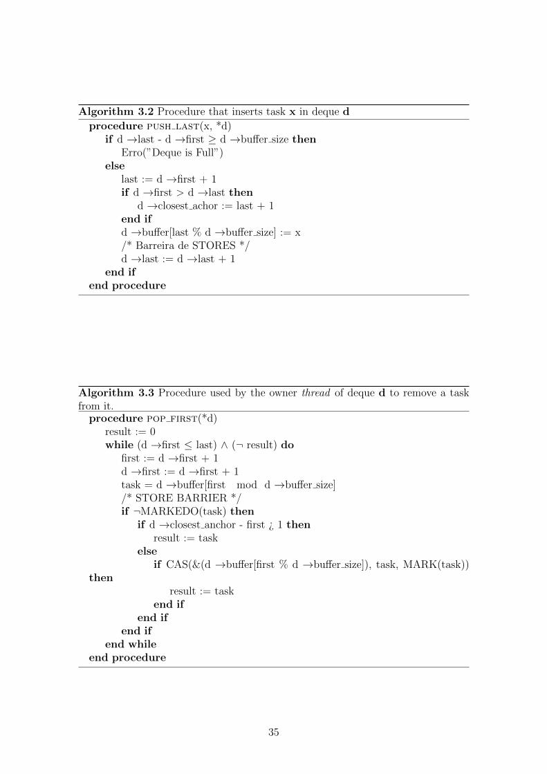
Algorithm 3.2 Procedure that inserts task x in deque d

procedure push last(x, *d)if d →last - d →first ≥ d →buffer size then

Erro(”Deque is Full”)else

last := d →first + 1if d →first > d →last then

d →closest achor := last + 1end ifd →buffer[last % d →buffer size] := x/* Barreira de STORES */d →last := d →last + 1

end ifend procedure

Algorithm 3.3 Procedure used by the owner thread of deque d to remove a taskfrom it.

procedure pop first(*d)result := 0while (d →first ≤ last) ∧ (¬ result) do

first := d →first + 1d →first := d →first + 1task = d →buffer[first mod d →buffer size]/* STORE BARRIER */if ¬MARKEDO(task) then

if d →closest anchor - first ¿ 1 thenresult := task

elseif CAS(&(d →buffer[first % d →buffer size]), task, MARK(task))

thenresult := task

end ifend if

end ifend while

end procedure

35

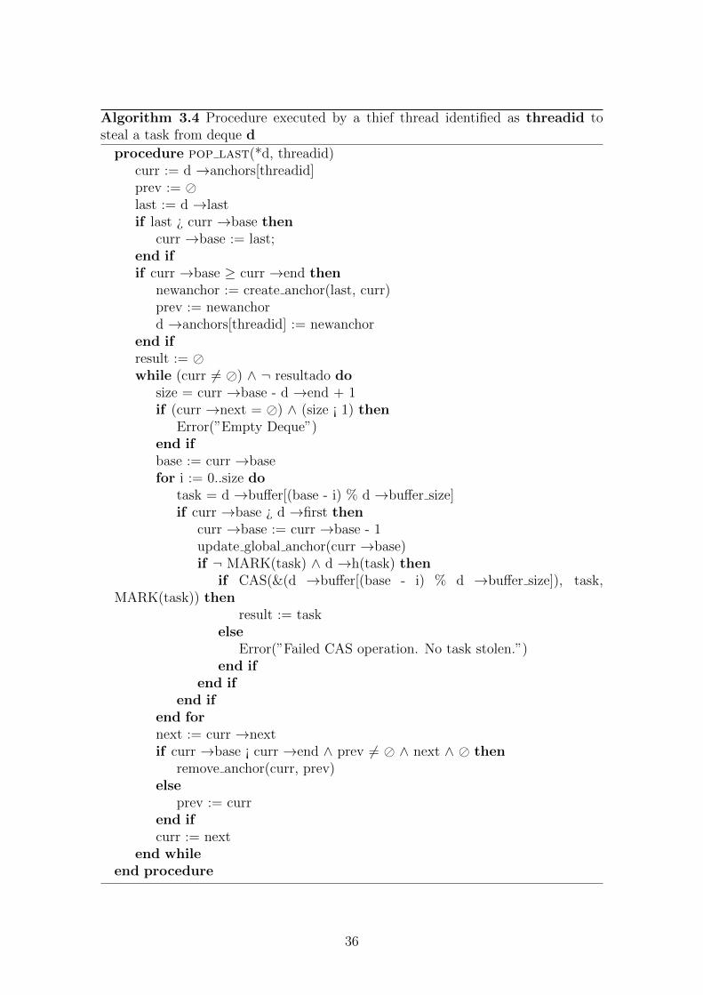
Algorithm 3.4 Procedure executed by a thief thread identified as threadid tosteal a task from deque d

procedure pop last(*d, threadid)curr := d →anchors[threadid]prev := �last := d →lastif last ¿ curr →base then

curr →base := last;end ifif curr →base ≥ curr →end then

newanchor := create anchor(last, curr)prev := newanchord →anchors[threadid] := newanchor

end ifresult := �while (curr 6= �) ∧ ¬ resultado do

size = curr →base - d →end + 1if (curr →next = �) ∧ (size ¡ 1) then

Error(”Empty Deque”)end ifbase := curr →basefor i := 0..size do

task = d →buffer[(base - i) % d →buffer size]if curr →base ¿ d →first then

curr →base := curr →base - 1update global anchor(curr →base)if ¬ MARK(task) ∧ d →h(task) then

if CAS(&(d →buffer[(base - i) % d →buffer size]), task,MARK(task)) then

result := taskelse

Error(”Failed CAS operation. No task stolen.”)end if

end ifend if

end fornext := curr →nextif curr →base ¡ curr →end ∧ prev 6= � ∧ next ∧ � then

remove anchor(curr, prev)else

prev := currend ifcurr := next

end whileend procedure

36

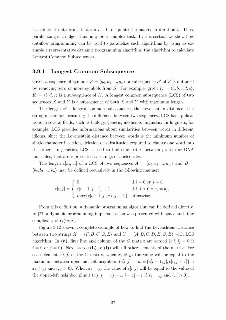
use different data from iteration i − 1 to update the matrix in iteration i. Thus,

parallelizing such algorithms may be a complex task. In this section we show how

dataflow programming can be used to parallelize such algorithms by using as ex-

ample a representative dynamic programming algorithm, the algorithm to calculate

Longest Common Subsequences.

3.9.1 Longest Common Subsequence

Given a sequence of symbols S = 〈a0, a1, ..., an〉, a subsequence S ′ of S is obtained

by removing zero or more symbols from S. For example, given K = 〈a, b, c, d, e〉,K ′ = 〈b, d, e〉 is a subsequence of K. A longest common subsequence (LCS) of two

sequences X and Y is a subsequence of both X and Y with maximum length.

The length of a longest common subsequence, the Levenshtein distance, is a

string metric for measuring the difference between two sequences. LCS has applica-

tions in several fields, such as biology, genetic, medicine, linguistic. In linguists, for

example, LCS provides informations about similarities between words in different

idioms, since the Levenshtein distance between words is the minimum number of

single-character insertion, deletion or substitution required to change one word into

the other. In genetics, LCS is used to find similarities between protein or DNA

molecules, that are represented as strings of nucleotides.

The length c[m, n] of a LCS of two sequences A = 〈a0, a1, ..., am〉 and B =

〈b0, b1, ..., bn〉 may be defined recursively in the following manner:

c[i, j] =

0 if i = 0 or j = 0,

c[i− 1, j − 1] + 1 if i, j > 0 ∧ ai = bj,

max{c[i− 1, j], c[i, j − 1]} otherwise.

From this definition, a dynamic programming algorithm can be derived directly.

In [27] a dynamic programming implementation was presented with space and time

complexity of O(m.n).

Figure 3.12 shows a complete example of how to find the Levenshtein Distance

between two strings X = 〈F,B,C,G,E〉 and Y = 〈A,B,C,D,E,G,E〉 with LCS

algorithm. In (a), first line and column of the C matrix are zeroed (c[i, j] = 0 if

i = 0 or j = 0). Next steps ((b) to (l)) will fill other elements of the matrix. For

each element c[i, j] of the C matrix, when xi 6= yj the value will be equal to the

maximum between uper and left neighbors (c[i, j] = max{c[i − 1, j], c[i, j − 1]} if

xi 6= yj and i, j > 0). When xi = yj the value of c[i, j] will be equal to the value of

the upper-left neighbor plus 1 (c[i, j] = c[i− 1, j − 1] + 1 if xi = yj and i, j > 0).

37

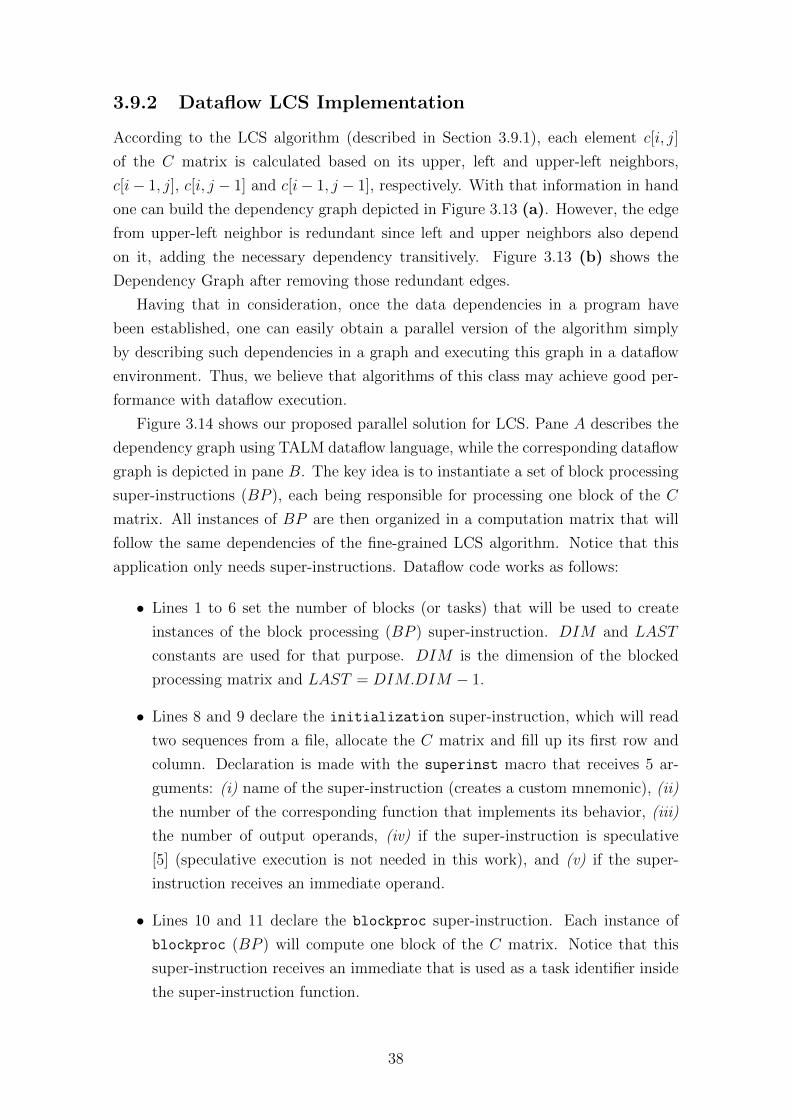
3.9.2 Dataflow LCS Implementation

According to the LCS algorithm (described in Section 3.9.1), each element c[i, j]

of the C matrix is calculated based on its upper, left and upper-left neighbors,

c[i− 1, j], c[i, j − 1] and c[i− 1, j − 1], respectively. With that information in hand

one can build the dependency graph depicted in Figure 3.13 (a). However, the edge

from upper-left neighbor is redundant since left and upper neighbors also depend

on it, adding the necessary dependency transitively. Figure 3.13 (b) shows the

Dependency Graph after removing those redundant edges.

Having that in consideration, once the data dependencies in a program have

been established, one can easily obtain a parallel version of the algorithm simply

by describing such dependencies in a graph and executing this graph in a dataflow

environment. Thus, we believe that algorithms of this class may achieve good per-

formance with dataflow execution.

Figure 3.14 shows our proposed parallel solution for LCS. Pane A describes the

dependency graph using TALM dataflow language, while the corresponding dataflow

graph is depicted in pane B. The key idea is to instantiate a set of block processing

super-instructions (BP ), each being responsible for processing one block of the C

matrix. All instances of BP are then organized in a computation matrix that will

follow the same dependencies of the fine-grained LCS algorithm. Notice that this

application only needs super-instructions. Dataflow code works as follows:

• Lines 1 to 6 set the number of blocks (or tasks) that will be used to create

instances of the block processing (BP ) super-instruction. DIM and LAST

constants are used for that purpose. DIM is the dimension of the blocked

processing matrix and LAST = DIM.DIM − 1.

• Lines 8 and 9 declare the initialization super-instruction, which will read

two sequences from a file, allocate the C matrix and fill up its first row and

column. Declaration is made with the superinst macro that receives 5 ar-

guments: (i) name of the super-instruction (creates a custom mnemonic), (ii)

the number of the corresponding function that implements its behavior, (iii)

the number of output operands, (iv) if the super-instruction is speculative

[5] (speculative execution is not needed in this work), and (v) if the super-

instruction receives an immediate operand.

• Lines 10 and 11 declare the blockproc super-instruction. Each instance of

blockproc (BP ) will compute one block of the C matrix. Notice that this

super-instruction receives an immediate that is used as a task identifier inside

the super-instruction function.

38

• Lines 12 and 13 declare the output super-instruction, which will write the

result and free memory.

• Lines 17 and 18 instantiate the initialization super-instruction. Instantia-

tion is done by using the custom mnemonic, followed by the instance identifier

and the list of input operands (the initialization super-instruction does

not have inputs).

• Lines 20 to 22 instantiate BP0, element (0, 0) of the computation matrix. This

element depends only on the initialization super-instruction.

• Lines 24 to 26 instantiate the first row of the computation matrix. Each one

of those BP instances will depend on their left neighbor.

• Lines 28 to 31 instantiate the first column of the computation matrix. Each

one of those BP instances will depend on their upper neighbor.

• Lines 33 to 39 instantiate the rest of the computation matrix. Each one of

those BP instances will depend on their upper and left neighbors.

• Lines 41 to 43 instantiate the output super-instruction, which will depend on

BPLAST .

3.9.3 LCS Experiments

To evaluate our solution, we have compiled the code presented in Section 3.9.2 to

execute on our Dataflow Runtime Environment: the Trebuchet [4, 5, 28]. We have

also prepared an OpenMP version that uses classic wavefront [29] to compute the C

matrix in parallel. Wavefront is a technique for parallelizing dynamic programming

algorithms where the elements in the diagonals of the matrix are calculated in par-

allel, since there is no dependency between them in the programs where wavefront is

successfully applied. Although wavefront can achieve good speed-ups, it relies on a

global barrier (after each diagonal is calculated). Our dataflow technique uses com-

pletetly distributed synchronization, so we intuitively expect our version to perform

better.

The machine used in our experiments has four AMD Six-Core OpteronTM8425

HE (2100 MHz) chips (24 cores), 128 GB of DDR-2 667MHz (32x4GB) RAM dual

channel and runs GNU/Linux (kernel 2.6.34.7-66 64 bits). The experiments were

executed 10 times for each scenario in order to remove discrepancies in the execution

time. Standard deviation was irrelevant (less than 0.4%).

To evaluate scalability inside a single chip and in the whole system, LCS is

executed with 2, 4, 6, 12, 18 and 24 cores. As input to the LCS application two

39

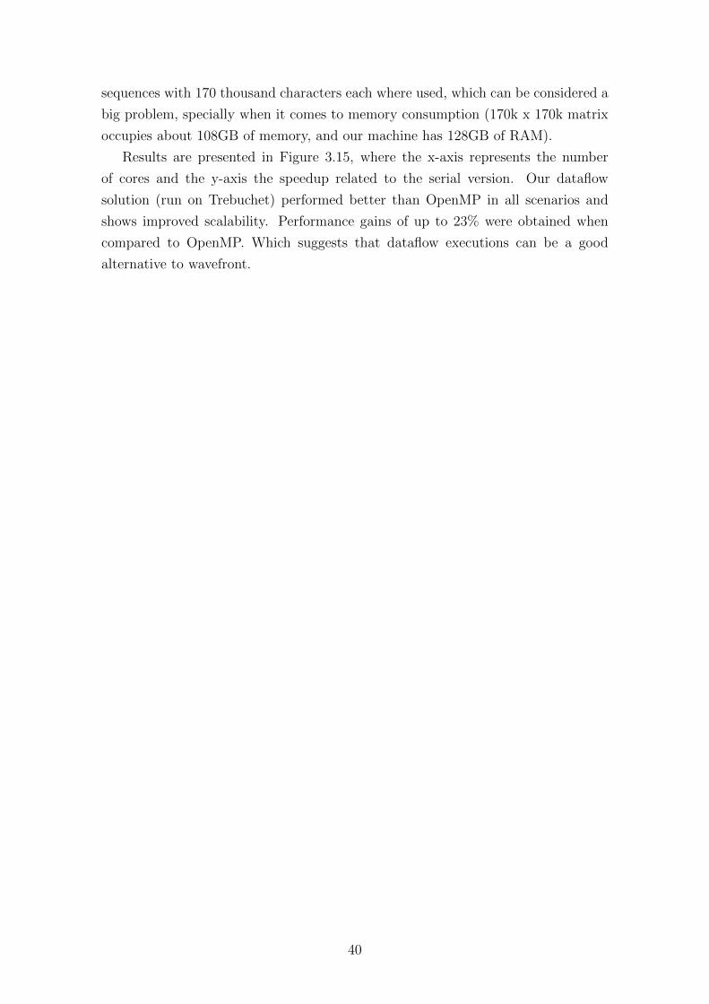
sequences with 170 thousand characters each where used, which can be considered a

big problem, specially when it comes to memory consumption (170k x 170k matrix

occupies about 108GB of memory, and our machine has 128GB of RAM).

Results are presented in Figure 3.15, where the x-axis represents the number

of cores and the y-axis the speedup related to the serial version. Our dataflow

solution (run on Trebuchet) performed better than OpenMP in all scenarios and

shows improved scalability. Performance gains of up to 23% were obtained when

compared to OpenMP. Which suggests that dataflow executions can be a good

alternative to wavefront.

40

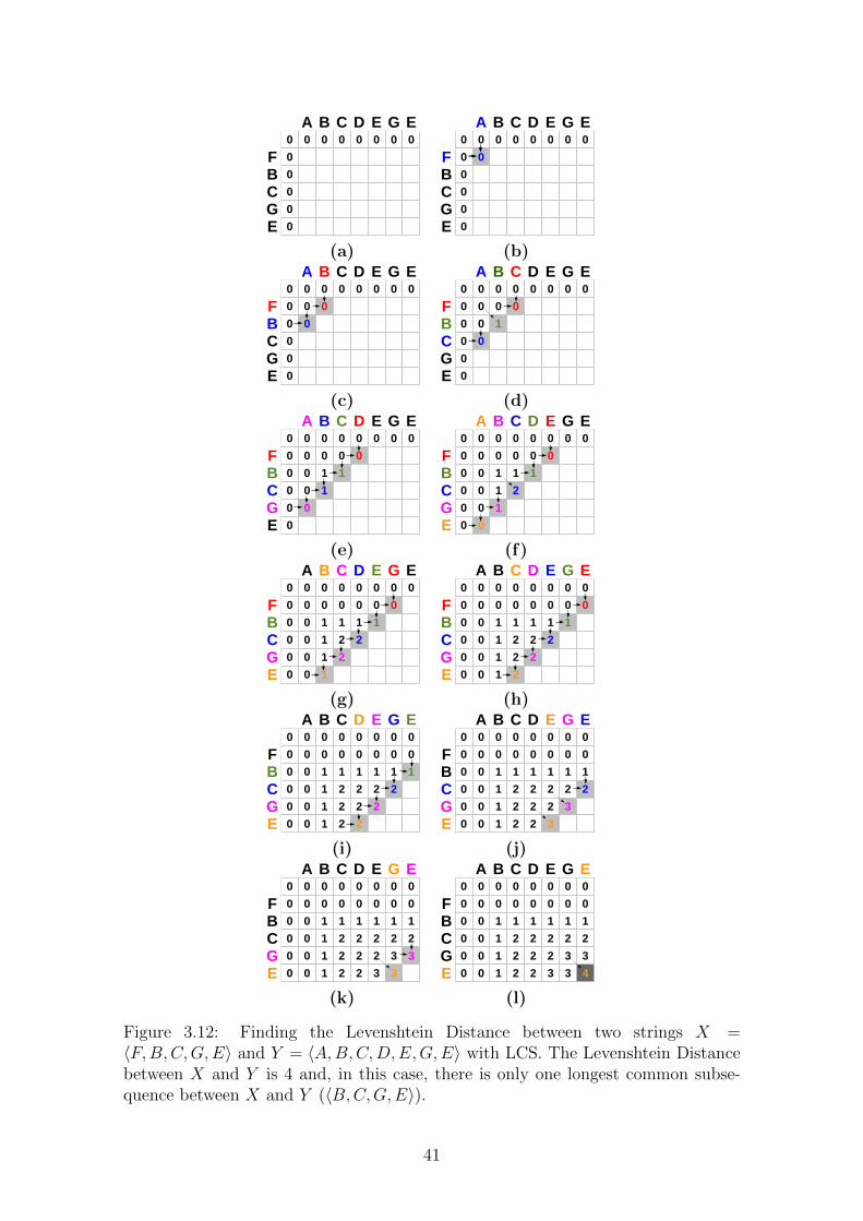
(a) (b)

(c) (d)

(e) (f)

(g) (h)

(i) (j)

(k) (l)

Figure 3.12: Finding the Levenshtein Distance between two strings X =〈F,B,C,G,E〉 and Y = 〈A,B,C,D,E,G,E〉 with LCS. The Levenshtein Distancebetween X and Y is 4 and, in this case, there is only one longest common subse-quence between X and Y (〈B,C,G,E〉).

41

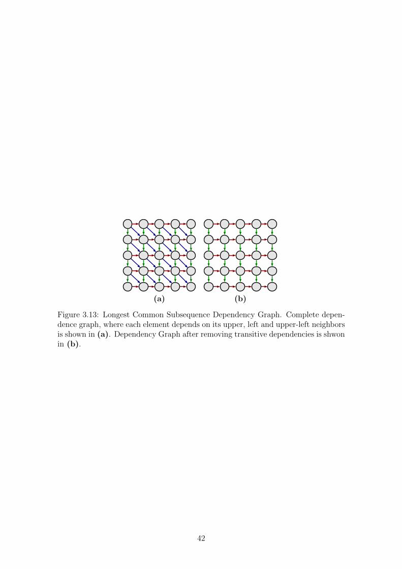
(a) (b)

Figure 3.13: Longest Common Subsequence Dependency Graph. Complete depen-dence graph, where each element depends on its upper, left and upper-left neighborsis shown in (a). Dependency Graph after removing transitive dependencies is shwonin (b).

42

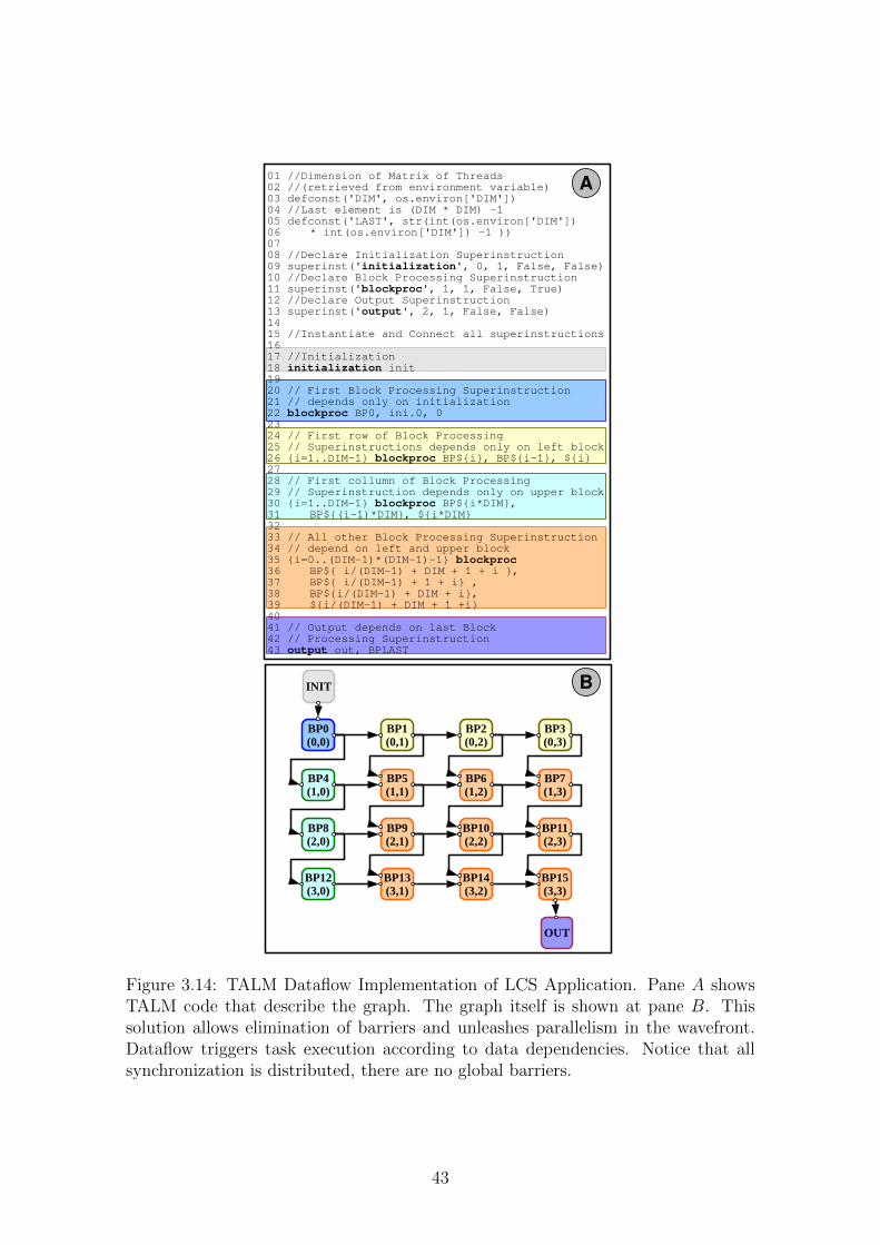
Figure 3.14: TALM Dataflow Implementation of LCS Application. Pane A showsTALM code that describe the graph. The graph itself is shown at pane B. Thissolution allows elimination of barriers and unleashes parallelism in the wavefront.Dataflow triggers task execution according to data dependencies. Notice that allsynchronization is distributed, there are no global barriers.

43

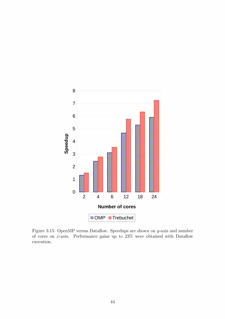
Figure 3.15: OpenMP versus Dataflow. Speedups are shown on y-axis and numberof cores on x-axis. Performance gains up to 23% were obtained with Dataflowexecution.

44

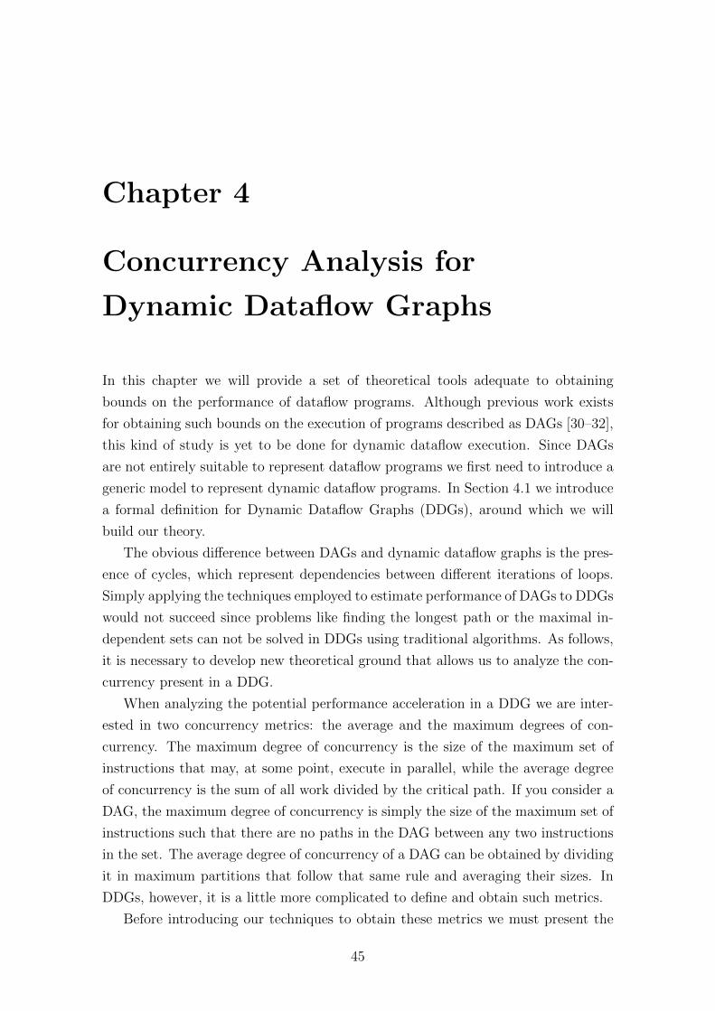
Chapter 4

Concurrency Analysis for

Dynamic Dataflow Graphs

In this chapter we will provide a set of theoretical tools adequate to obtaining

bounds on the performance of dataflow programs. Although previous work exists

for obtaining such bounds on the execution of programs described as DAGs [30–32],

this kind of study is yet to be done for dynamic dataflow execution. Since DAGs

are not entirely suitable to represent dataflow programs we first need to introduce a

generic model to represent dynamic dataflow programs. In Section 4.1 we introduce

a formal definition for Dynamic Dataflow Graphs (DDGs), around which we will

build our theory.

The obvious difference between DAGs and dynamic dataflow graphs is the pres-

ence of cycles, which represent dependencies between different iterations of loops.

Simply applying the techniques employed to estimate performance of DAGs to DDGs

would not succeed since problems like finding the longest path or the maximal in-

dependent sets can not be solved in DDGs using traditional algorithms. As follows,

it is necessary to develop new theoretical ground that allows us to analyze the con-

currency present in a DDG.

When analyzing the potential performance acceleration in a DDG we are inter-

ested in two concurrency metrics: the average and the maximum degrees of con-

currency. The maximum degree of concurrency is the size of the maximum set of

instructions that may, at some point, execute in parallel, while the average degree

of concurrency is the sum of all work divided by the critical path. If you consider a

DAG, the maximum degree of concurrency is simply the size of the maximum set of

instructions such that there are no paths in the DAG between any two instructions

in the set. The average degree of concurrency of a DAG can be obtained by dividing

it in maximum partitions that follow that same rule and averaging their sizes. In

DDGs, however, it is a little more complicated to define and obtain such metrics.

Before introducing our techniques to obtain these metrics we must present the

45

motivation behind them. Understanding the need to obtain the maximum degree of

concurrency is straightforward, since it clearly represents the maximum number of

processing elements that can be used to execute the graph. If you allocate processing

elements beyond that number, it is certain that the computation will never use all

computational resources, representing a waste of energy and CPU time. The average

degree of concurrency can be shown to be equal to the maximum speed-up that can

be obtained by executing the graph in an ideal system with infinite resources, optimal

scheduling and zero overhead. We will also present a lower bound for the speed-up,

which was not yet mentioned because its calculation is based on the average degree

of concurrency and because it was introduced by Arora et al. [17], although in

previous work it was only applied to DAGs.

Static scheduling is another area in which extensive work was done on DAGs

[16], [33], [14], [34], but was not profundly addressed when it comes do dynamic

dataflow. In the end of this chapter we will present a variation on Algorithm 3.1

that takes into account the possibility for two instructions to be iteration-dependent

(i.e. have dependencies between them inside the same iteration of the loop) and, at

the same time, iteration-independent (i.e. have no dependencies between instances

of different iterations).

The rest of this chapter is organized as follows: (i) In Section 4.1 we introduce

a formal definition of DDGs; (ii) in Section 4.2 we present an algorithm to obtain

the maximum degree of concurrency in a DDG; (iii) in Section 4.3 we define and

show how to calculate the maximum speed-up of a DDG; (iv) in Section 4.5 we

present a variation of Algorithm 3.1 that applies the theory presented previously in

this chapter; (v) in Section 4.6 we model and compare two different pipelines as an

example of how our theory can be applied and (vi) in Section 4.7 we present a few

experiments done to validate the theory.

4.1 Definition of Dynamic Dataflow Graphs

First of all, we shall present a definition for Dynamic Dataflow Graphs (DDGs) such

that the theory presented for them can be applied not only to our work, but also

to any model that employs dynamic dataflow execution. For simplicity, we propose

a set of restrictions for the programs represented as DDGs, but it is possible to

generalize the model and apply all the work presented in the rest of the chapter to

programs that do not comply with the restrictions. The restrictions are as follows:

1. The only kind of conditional execution are loop bodies (whose condition is the

loop test expression).

2. There are no nested loops.

46

3. Dependencies between different iterations only exist between two consecutive

iterations (from the i-th to the (i+ 1)-th iteration).

Although these restrictions may seem too hard at first, we will show throught

this chapter that the study of DDGs allows us to analyze an important aspect that is

unique to dynamic dataflow, the execution of the cycles that represent loops. Also,

as mentioned, it is not hard to eliminate these restrictions and apply the methods

presented to programs that can not be represented in a graph that strictly follows

DDG convention.

A DDG is a tuple D = (I, E,R,W ) where:

• I is the set of instructions in the program.

• E is the set of edges, ordered pairs (a, b) such that {a, b} ⊆ I and the instruc-

tion b consumes data produced by a and a is not inside a loop or a and b are

inside a loop and this dependency occurs in the same iteration, i.e. the data

b consumes in iteration i is produced by a also in iteration i.

• R is the set of return edges, they are also ordered pairs, just like the edges in E,

but they describe dependencies between different iterations, consequently they

only happen when both instructions are inside a loop. A return edge r = (a, b)

describes that b during iteration i of the loop consumes data produced by a in

the iteration i− 1.

• W is the set of weights of the instructions, where the weight represents the

granularity of that instruction, since granularities may vary, as discussed in

Chapter 3.

4.2 Maximum Degree of Concurrency in a DDG

We call the maximum degree of concurrency in a DDG the largest set of instructions

that can, at some point, be executing in parallel. In DAGs, it is direct to verify

that these independent sets must be such that there is no path in the DAG between

any pair of instructions in the set. But since we are dealing with DDGs things get

a little bit more complicated, as you can have dependencies (or the lack of them)

between different iterations.

In order to delve deeper into the problem we should first introduce additional

notation. If v is an instruction inside the body of a loop, we call v(i) the instance

of v executed in the i-th iteration of the loop. Let us also indicate by u(i) → v(j)

that v(j) depends on u(i) and by u(i) 6→ v(j) that v(j) does not depend on u(i).

47

a

b

c

a

b

c

a

b

c

(a) (b) (c)

Figure 4.1: Example of DDGs whose maximum degree of concurrency are 1, 2 andunbounded, respectively. The dashed arcs represent return edges.

In the DDG of Figure 4.1a, b(i) → c(i) and c(i − 1) → b(i) (observe the return

edge, represented as a dashed arc), for i > 1, so, transitively b(i− 1)→ b(i). In this

case, at any point it is only possible to have exactly one instruction running at a

time. We say the maximum degree of concurrency for this DDG is 1. Now consider

the DDG of Figure 4.1b. This time, b(i)→ c(i), b(i− 1)→ b(i) and c(i− 1)→ c(i),

but c(i−1) 6→ b(i). So, potentially, b(i) and c(i−1) can execute in parallel, yielding

a maximum degree of concurrency of 2 for this DDG.

In the DDG of Figure 4.1c c(i) depends on b(i) and b(i) depends on b(i − 1)

(observe the return edge, represented as a dashed arc), but c(i) does not depend

on c(i − 1). For instance, it would be possible for c(i) and c(i + 1) to execute

in parallel. As a matter of fact, if b runs fast enough it would be possible to

have potentially infinite instances of c executing in parallel. We say that DDGs

with this characteristic have an unbounded maximum degree of concurrency, since,

given the right conditions, it is possible to have an ubounded number of instructions

executing in parallel. The importance of this metric lies in the decision of resource

allocation for the execution of the dynamic dataflow graph. If the maximum degree

of concurrency Cmax of a DDG is bounded, at any time during the execution of the

DDG no more than Cmax processing elements will be busy. Therefore, allocating

more than Cmax PEs to execute that DDG would be potentially wasteful.

Now that we have introduced the concept of maximum degree of concurrency

in DDGs we shall present an algorithm to calculate it. Basically, the technique

employed by the algorithm presented in this chapter consists of applying a transfor-

mation similar to loop unrolling [35] to the DDG.

48

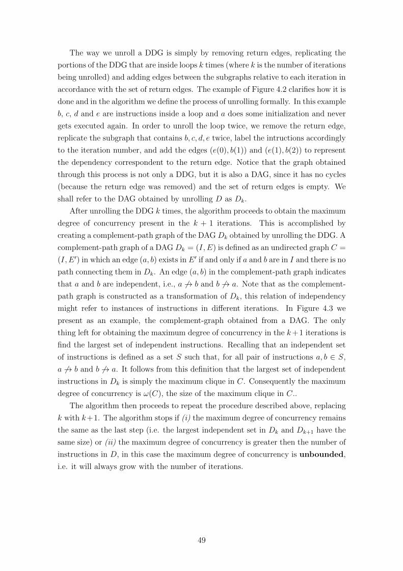
The way we unroll a DDG is simply by removing return edges, replicating the

portions of the DDG that are inside loops k times (where k is the number of iterations

being unrolled) and adding edges between the subgraphs relative to each iteration in

accordance with the set of return edges. The example of Figure 4.2 clarifies how it is

done and in the algorithm we define the process of unrolling formally. In this example

b, c, d and e are instructions inside a loop and a does some initialization and never

gets executed again. In order to unroll the loop twice, we remove the return edge,

replicate the subgraph that contains b, c, d, e twice, label the intructions accordingly

to the iteration number, and add the edges (e(0), b(1)) and (e(1), b(2)) to represent

the dependency correspondent to the return edge. Notice that the graph obtained

through this process is not only a DDG, but it is also a DAG, since it has no cycles

(because the return edge was removed) and the set of return edges is empty. We

shall refer to the DAG obtained by unrolling D as Dk.

After unrolling the DDG k times, the algorithm proceeds to obtain the maximum

degree of concurrency present in the k + 1 iterations. This is accomplished by

creating a complement-path graph of the DAG Dk obtained by unrolling the DDG. A

complement-path graph of a DAG Dk = (I, E) is defined as an undirected graph C =

(I, E ′) in which an edge (a, b) exists in E ′ if and only if a and b are in I and there is no

path connecting them in Dk. An edge (a, b) in the complement-path graph indicates

that a and b are independent, i.e., a 6→ b and b 6→ a. Note that as the complement-

path graph is constructed as a transformation of Dk, this relation of independency

might refer to instances of instructions in different iterations. In Figure 4.3 we

present as an example, the complement-graph obtained from a DAG. The only

thing left for obtaining the maximum degree of concurrency in the k+1 iterations is

find the largest set of independent instructions. Recalling that an independent set

of instructions is defined as a set S such that, for all pair of instructions a, b ∈ S,

a 6→ b and b 6→ a. It follows from this definition that the largest set of independent

instructions in Dk is simply the maximum clique in C. Consequently the maximum

degree of concurrency is ω(C), the size of the maximum clique in C..

The algorithm then proceeds to repeat the procedure described above, replacing

k with k+1. The algorithm stops if (i) the maximum degree of concurrency remains

the same as the last step (i.e. the largest independent set in Dk and Dk+1 have the

same size) or (ii) the maximum degree of concurrency is greater then the number of

instructions in D, in this case the maximum degree of concurrency is unbounded,

i.e. it will always grow with the number of iterations.

49

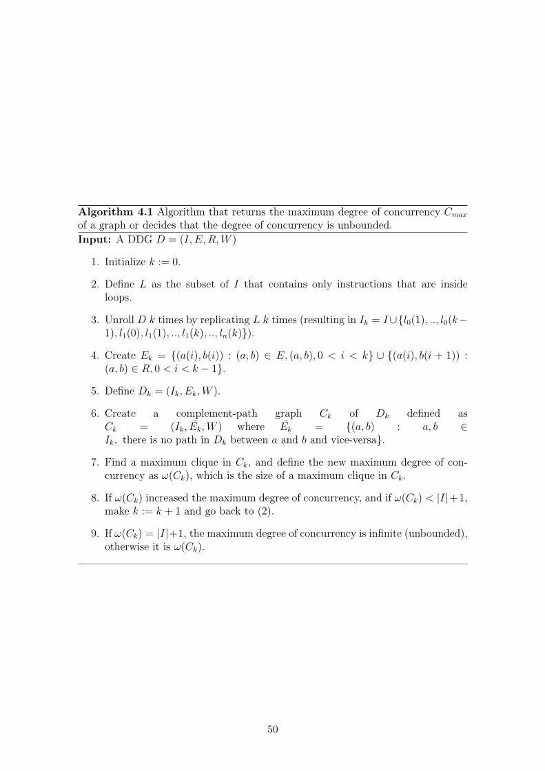
Algorithm 4.1 Algorithm that returns the maximum degree of concurrency Cmax

of a graph or decides that the degree of concurrency is unbounded.

Input: A DDG D = (I, E,R,W )

1. Initialize k := 0.

2. Define L as the subset of I that contains only instructions that are insideloops.

3. Unroll D k times by replicating L k times (resulting in Ik = I∪{l0(1), .., l0(k−1), l1(0), l1(1), .., l1(k), .., ln(k)}).

4. Create Ek = {(a(i), b(i)) : (a, b) ∈ E, (a, b), 0 < i < k} ∪ {(a(i), b(i + 1)) :(a, b) ∈ R, 0 < i < k − 1}.

5. Define Dk = (Ik, Ek,W ).

6. Create a complement-path graph Ck of Dk defined asCk = (Ik, Ek,W ) where Ek = {(a, b) : a, b ∈Ik, there is no path in Dk between a and b and vice-versa}.

7. Find a maximum clique in Ck, and define the new maximum degree of con-currency as ω(Ck), which is the size of a maximum clique in Ck.

8. If ω(Ck) increased the maximum degree of concurrency, and if ω(Ck) < |I|+1,make k := k + 1 and go back to (2).

9. If ω(Ck) = |I|+1, the maximum degree of concurrency is infinite (unbounded),otherwise it is ω(Ck).

50

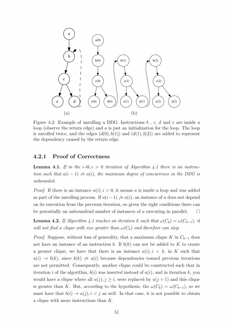
a

b

c

de

a(0)

b(0)

c(0)

d(0)e(0)

b(1)

c(1)

d(1)e(1)

b(2)

c(2)

d(2)e(2)

(a) (b)

Figure 4.2: Example of unrolling a DDG. Instructions b , c, d and e are inside aloop (observe the return edge) and a is just an initialization for the loop. The loopis unrolled twice, and the edges (d(0), b(1)) and (d(1), b(2)) are added to representthe dependency caused by the return edge.

4.2.1 Proof of Correctness

Lemma 4.1. If in the i-th, i > 0 iteration of Algorithm 4.1 there is an instruc-

tion such that a(i − 1) 6→ a(i), the maximum degree of concurrence in the DDG is

unbounded.

Proof. If there is an instance a(i), i > 0, it means a is inside a loop and was added

as part of the unrolling process. If a(i−1) 6→ a(i), an instance of a does not depend

on its execution from the previous iteration, so given the right conditions there can

be potentially an unboundend number of instances of a executing in parallel.

Lemma 4.2. If Algorithm 4.1 reaches an iteration k such that ω(Ck) = ω(Ck−1), it

will not find a clique with size greater than ω(Ck) and therefore can stop.

Proof. Suppose, without loss of generality, that a maximum clique K in Ck−1 does

not have an instance of an instruction b. If b(k) can not be added to K to create

a greater clique, we have that there is an instance a(i), i < k, in K such that

a(i) → b(k), since b(k) 6→ a(i) because dependencies toward previous iterations

are not permitted. Consequently, another clique could be constructed such that in

iteration i of the algorithm, b(i) was inserted instead of a(i), and in iteration k, you

would have a clique where all u(j), j ≥ i, were replaced by u(j + 1) and this clique

is greater than K. But, according to the hypothesis, the ω(Ck) = ω(Ck−1), so we

must have that b(i) → a(j), i < j as well. In that case, it is not possible to obtain

a clique with more instructions than K.

51

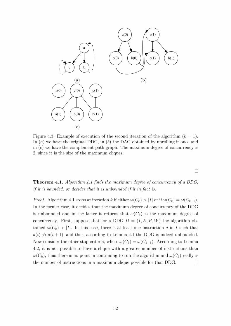
a

bc

a(0)

b(0)c(0)

a(1)

c(1) b(1)

(a) (b)

a(0) c(0)

a(1) b(0) b(1)

c(1)

(c)

Figure 4.3: Example of execution of the second iteration of the algorithm (k = 1).In (a) we have the original DDG, in (b) the DAG obtained by unrolling it once andin (c) we have the complement-path graph. The maximum degree of concurrency is2, since it is the size of the maximum cliques.

Theorem 4.1. Algorithm 4.1 finds the maximum degree of concurrency of a DDG,

if it is bounded, or decides that it is unbounded if it in fact is.

Proof. Algorithm 4.1 stops at iteration k if either ω(Ck) > |I| or if ω(Ck) = ω(Ck−1).

In the former case, it decides that the maximum degree of concurrency of the DDG

is unbounded and in the latter it returns that ω(Ck) is the maximum degree of

concurrency. First, suppose that for a DDG D = (I, E,R,W ) the algorithm ob-

tained ω(Ck) > |I|. In this case, there is at least one instruction a in I such that

a(i) 6→ a(i + 1), and thus, according to Lemma 4.1 the DDG is indeed unbounded.

Now consider the other stop criteria, where ω(Ck) = ω(Ck−1). According to Lemma

4.2, it is not possible to have a clique with a greater number of instructions than

ω(Ck), thus there is no point in continuing to run the algorithm and ω(Ck) really is

the number of instructions in a maximum clique possible for that DDG.

52

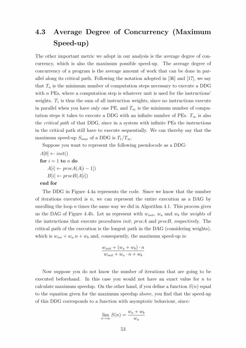
4.3 Average Degree of Concurrency (Maximum

Speed-up)

The other important metric we adopt in our analysis is the average degree of con-

currency, which is also the maximum possible speed-up. The average degree of

concurrency of a program is the average amount of work that can be done in par-

allel along its critical path. Following the notation adopted in [36] and [17], we say

that Tn is the minimum number of computation steps necessary to execute a DDG

with n PEs, where a computation step is whatever unit is used for the instructions’

weights. T1 is thus the sum of all instruction weights, since no instructions execute

in parallel when you have only one PE, and T∞ is the minimum number of compu-

tation steps it takes to execute a DDG with an infinite number of PEs. T∞ is also

the critical path of that DDG, since in a system with infinite PEs the instructions

in the critical path still have to execute sequentially. We can thereby say that the

maximum speed-up Smax of a DDG is T1/T∞.

Suppose you want to represent the following pseudocode as a DDG:

A[0]← init()

for i = 1 to n do

A[i]← procA(A[i− 1])

B[i]← procB(A[i])

end for

The DDG in Figure 4.4a represents the code. Since we know that the number

of iterations executed is n, we can represent the entire execution as a DAG by

unrolling the loop n times the same way we did in Algorithm 4.1. This process gives

us the DAG of Figure 4.4b. Let us represent with winit, wa and wb the weights of

the instructions that execute procedures init, procA and procB, respectively. The

critical path of the execution is the longest path in the DAG (considering weights),

which is wini + wa.n+ wb and, consequently, the maximum speed-up is:

winit + (wa + wb) · nwinit + wa · n+ wb

Now suppose you do not know the number of iterations that are going to be

executed beforehand. In this case you would not have an exact value for n to

calculate maximum speedup. On the other hand, if you define a function S(n) equal

to the equation given for the maximum speedup above, you find that the speed-up

of this DDG corresponds to a function with asymptotic behaviour, since:

limn→∞

S(n) =wa + wb

wa

53

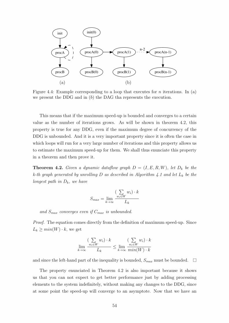
init

procA

procB

init(0)

procA(0)

procB(0)

procA(1) procA(n-1) n-2

procB(1) procB(n-1)

(a) (b)

Figure 4.4: Example corresponding to a loop that executes for n iterations. In (a)we present the DDG and in (b) the DAG tha represents the execution.

This means that if the maximum speed-up is bounded and converges to a certain

value as the number of iterations grows. As will be shown in theorem 4.2, this

property is true for any DDG, even if the maximum degree of concurrency of the

DDG is unbounded. And it is a very important property since it is often the case in

which loops will run for a very large number of iterations and this property allows us

to estimate the maximum speed-up for them. We shall thus enunciate this property

in a theorem and then prove it.

Theorem 4.2. Given a dynamic dataflow graph D = (I, E,R,W ), let Dk be the

k-th graph generated by unrolling D as described in Algorithm 4.1 and let Lk be the

longest path in Dk, we have

Smax = limk→∞

(∑

wi∈Wwi) · k

Lk

and Smax converges even if Cmax is unbounded.

Proof. The equation comes directly from the definition of maximum speed-up. Since

Lk ≥ min(W ) · k, we get

limk→∞

(∑

wi∈Wwi) · k

Lk

≤ limk→∞

(∑

wi∈Wwi) · k

min(W ) · k

and since the left-hand part of the inequality is bounded, Smax must be bounded.

The property enunciated in Theorem 4.2 is also important because it shows

us that you can not expect to get better performance just by adding processing

elements to the system indefinitely, without making any changes to the DDG, since

at some point the speed-up will converge to an asymptote. Now that we have an

54

upper bound for speed-up, it can also be useful to have a lower bound for it as well,

considering that it would provide us the tools to project the expected performance

of a DDG. In Section 4.4 we discuss an upper bound on the number of computation

steps it takes to execute a DDG, which will give us a lower bound for speed-up in

an ideal system.

4.4 Lower Bound for Speed-up

Blumofe et al. [30] showed that the number of computation steps for any computa-

tion with total work T1 and critical path length T∞ is at most T1/P+T∞ in a system

with P processors and greedy scheduling. The definition of greedy scheduling is

that at each computation step the number of instructions being executed is the

minimum between the number of instructions that are ready and the number of

processors available.

This bound fits our target executions, since we know how to calculate T1 and T∞

for DDGs and dataflow runtimes with work-stealing can be characterized as having

greedy scheduling policies. We therefore shall use that upper bound on computation

steps to model the performance of DDGs.

Actually, since we are interested in modeling the potential speed-up of a DDG,

the expression we must use is the total amount of work T1 divided by the upper

bound on computation steps, which will give us a lower bound on speed-up:

Smin =T1

T1/P + T∞

It is important to be very clear about what this lower bound describes in order

to understand the behaviour of the experimental results we present in the end of

this chapter in comparison with the theoretical analysis. The upper bound on time

proved by Blumofe et al. takes into consideration the number of computation steps

it takes to execute the work using a greedy scheduling. Basically, it means that

overheads of the runtime are not taken into account and there is the assumption

that the system never fails to schedule for execution all instructions that are ready,

if there is a processor available. Clearly that is not the situation we face when doing

actual experimentation, since the dataflow runtime occurs in overheads besides the

ones inherent to the computation being done. Consequently, this lower bound on

speed-up Smin will serve us more as a guideline of how much the dataflow runtime

overheads are influencing overall performance, while the upper bound Smax indicates

the potential of the DDG. If the performance obtained in an experiment falls below

Smin that indicates that the overheads of the runtime for that execution ought to

be studied and optimized.

55

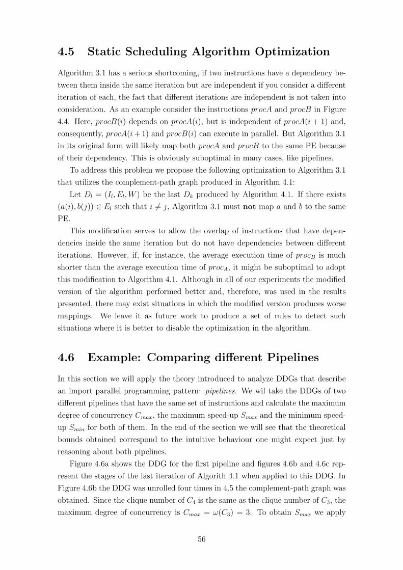
4.5 Static Scheduling Algorithm Optimization

Algorithm 3.1 has a serious shortcoming, if two instructions have a dependency be-

tween them inside the same iteration but are independent if you consider a different

iteration of each, the fact that different iterations are independent is not taken into

consideration. As an example consider the instructions procA and procB in Figure

4.4. Here, procB(i) depends on procA(i), but is independent of procA(i + 1) and,

consequently, procA(i+ 1) and procB(i) can execute in parallel. But Algorithm 3.1

in its original form will likely map both procA and procB to the same PE because

of their dependency. This is obviously suboptimal in many cases, like pipelines.

To address this problem we propose the following optimization to Algorithm 3.1

that utilizes the complement-path graph produced in Algorithm 4.1:

Let Dl = (Il, El,W ) be the last Dk produced by Algorithm 4.1. If there exists

(a(i), b(j)) ∈ El such that i 6= j, Algorithm 3.1 must not map a and b to the same

PE.

This modification serves to allow the overlap of instructions that have depen-

dencies inside the same iteration but do not have dependencies between different

iterations. However, if, for instance, the average execution time of procB is much

shorter than the average execution time of procA, it might be suboptimal to adopt

this modification to Algorithm 4.1. Although in all of our experiments the modified

version of the algorithm performed better and, therefore, was used in the results

presented, there may exist situations in which the modified version produces worse

mappings. We leave it as future work to produce a set of rules to detect such

situations where it is better to disable the optimization in the algorithm.

4.6 Example: Comparing different Pipelines

In this section we will apply the theory introduced to analyze DDGs that describe

an import parallel programming pattern: pipelines. We wil take the DDGs of two

different pipelines that have the same set of instructions and calculate the maximum

degree of concurrency Cmax, the maximum speed-up Smax and the minimum speed-

up Smin for both of them. In the end of the section we will see that the theoretical

bounds obtained correspond to the intuitive behaviour one might expect just by

reasoning about both pipelines.

Figure 4.6a shows the DDG for the first pipeline and figures 4.6b and 4.6c rep-

resent the stages of the last iteration of Algorith 4.1 when applied to this DDG. In

Figure 4.6b the DDG was unrolled four times in 4.5 the complement-path graph was

obtained. Since the clique number of C4 is the same as the clique number of C3, the

maximum degree of concurrency is Cmax = ω(C3) = 3. To obtain Smax we apply

56

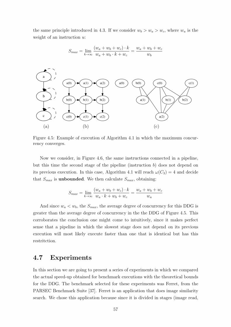
the same principle introduced in 4.3. If we consider wb > wa > wc, where wu is the

weight of an instruction u:

Smax = limk→∞

(wa + wb + wc) · kwa + wb · k + wc

=wa + wb + wc

wb

a

b

c

a(0)

b(0)

a(1)

c(0)

b(1)

c(1)

a(2)

b(2)

c(2)

a(0) b(0)

a(1)

a(2)

b(1)

c(0)

b(2)

c(1)

(a) (b) (c)

Figure 4.5: Example of execution of Algorithm 4.1 in which the maximum concur-rency converges.

Now we consider, in Figure 4.6, the same instructions connected in a pipeline,

but this time the second stage of the pipeline (instruction b) does not depend on

its previous execution. In this case, Algorithm 4.1 will reach ω(C3) = 4 and decide

that Smax is unbounded. We then calculate Smax, obtaining:

Smax = limk→∞

(wa + wb + wc) · kwa · k + wb + wc

=wa + wb + wc

wa

And since wa < wb, the Smax, the average degree of concurrency for this DDG is

greater than the average degree of concurrency in the the DDG of Figure 4.5. This

corroborates the conclusion one might come to intuitively, since it makes perfect

sense that a pipeline in which the slowest stage does not depend on its previous

execution will most likely execute faster than one that is identical but has this

restritction.

4.7 Experiments

In this section we are going to present a series of experiments in which we compared

the actual speed-up obtained for benchmark executions with the theoretical bounds

for the DDG. The benchmark selected for these experiments was Ferret, from the

PARSEC Benchmark Suite [37]. Ferret is an application that does image similarity

search. We chose this application because since it is divided in stages (image read,

57

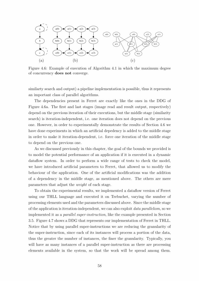
a

b

c

a(0)

b(0)

a(1)

c(0) c(1)

b(1)

a(2)

c(2)

b(2)

a(3)

c(3)

b(3)

a(0) b(0)

a(1)

a(2)

b(1)

b(2)

c(0)

a(3) b(3)

c(1)c(2)

(a) (b) (c)

Figure 4.6: Example of execution of Algorithm 4.1 in which the maximum degreeof concurrency does not converge.

similarty search and output) a pipeline implementation is possible, thus it represents

an important class of parallel algorithms.

The dependencies present in Ferret are exactly like the ones in the DDG of

Figure 4.6a. The first and last stages (image read and result output, respectively)

depend on the previous iteration of their executions, but the middle stage (similarity

search) is iteration-independent, i.e. one iteration does not depend on the previous

one. However, in order to experimentally demonstrate the results of Section 4.6 we

have done experiments in which an artificial depedency is added to the middle stage

in order to make it iteration-dependent, i.e. force one iteration of the middle stage

to depend on the previous one.

As we discussed previously in this chapter, the goal of the bounds we provided is

to model the potential performance of an application if it is executed in a dynamic

dataflow system. In order to perform a wide range of tests to check the model,

we have introduced artificial parameters to Ferret, that allowed us to modify the

behaviour of the application. One of the artificial modifications was the addition

of a dependency in the middle stage, as mentioned above. The others are mere

parameters that adjust the weight of each stage.

To obtain the experimental results, we implemented a dataflow version of Ferret

using our THLL language and executed it on Trebuchet, varying the number of

processing elements used and the parameters discussed above. Since the middle stage

of the application is iteration-independent, we can also exploit data parallelism, so we

implemented it as a parallel super-instruction, like the example presented in Section

3.5. Figure 4.7 shows a DDG that represents our implementation of Ferret in THLL.

Notice that by using parallel super-instructions we are reducing the granularity of

the super-instruction, since each of its instances will process a portion of the data,

thus the greater the number of instances, the finer the granularity. Typically, you

will have as many instances of a parallel super-instruction as there are processing

elements available in the system, so that the work will be spread among them.

58

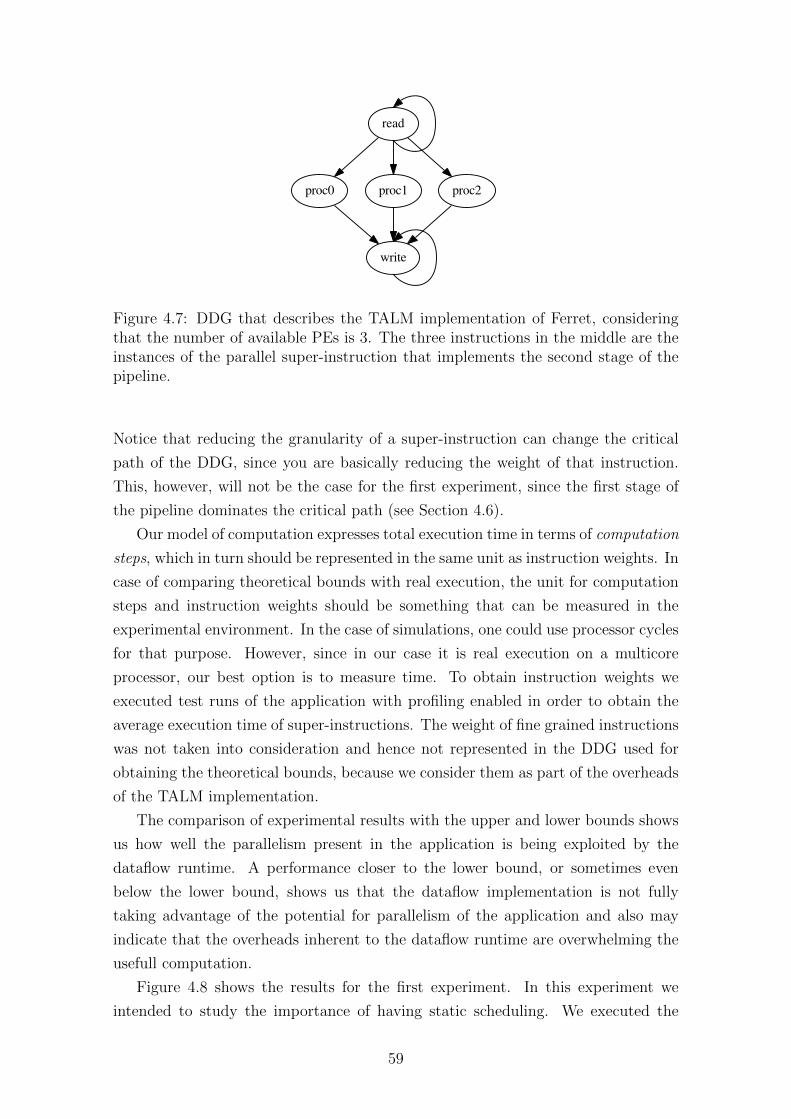
read

proc0 proc1 proc2

write

Figure 4.7: DDG that describes the TALM implementation of Ferret, consideringthat the number of available PEs is 3. The three instructions in the middle are theinstances of the parallel super-instruction that implements the second stage of thepipeline.

Notice that reducing the granularity of a super-instruction can change the critical

path of the DDG, since you are basically reducing the weight of that instruction.

This, however, will not be the case for the first experiment, since the first stage of

the pipeline dominates the critical path (see Section 4.6).

Our model of computation expresses total execution time in terms of computation

steps, which in turn should be represented in the same unit as instruction weights. In

case of comparing theoretical bounds with real execution, the unit for computation

steps and instruction weights should be something that can be measured in the

experimental environment. In the case of simulations, one could use processor cycles

for that purpose. However, since in our case it is real execution on a multicore

processor, our best option is to measure time. To obtain instruction weights we

executed test runs of the application with profiling enabled in order to obtain the

average execution time of super-instructions. The weight of fine grained instructions

was not taken into consideration and hence not represented in the DDG used for

obtaining the theoretical bounds, because we consider them as part of the overheads

of the TALM implementation.

The comparison of experimental results with the upper and lower bounds shows

us how well the parallelism present in the application is being exploited by the

dataflow runtime. A performance closer to the lower bound, or sometimes even

below the lower bound, shows us that the dataflow implementation is not fully

taking advantage of the potential for parallelism of the application and also may

indicate that the overheads inherent to the dataflow runtime are overwhelming the

usefull computation.

Figure 4.8 shows the results for the first experiment. In this experiment we

intended to study the importance of having static scheduling. We executed the

59

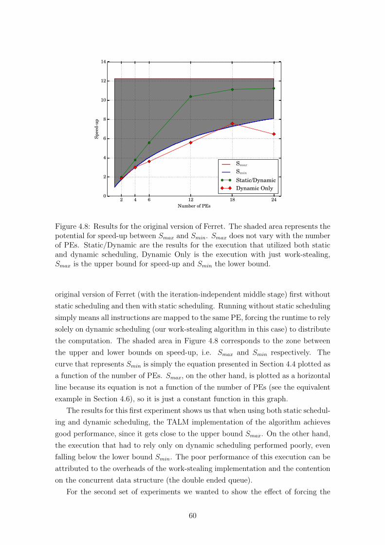
241812642Number of PEs

0

2

4

6

8

10

12

14

Spee

d-up

SmaxSminStatic/DynamicDynamic Only

Figure 4.8: Results for the original version of Ferret. The shaded area represents thepotential for speed-up between Smax and Smin. Smax does not vary with the numberof PEs. Static/Dynamic are the results for the execution that utilized both staticand dynamic scheduling, Dynamic Only is the execution with just work-stealing,Smax is the upper bound for speed-up and Smin the lower bound.

original version of Ferret (with the iteration-independent middle stage) first without

static scheduling and then with static scheduling. Running without static scheduling

simply means all instructions are mapped to the same PE, forcing the runtime to rely

solely on dynamic scheduling (our work-stealing algorithm in this case) to distribute

the computation. The shaded area in Figure 4.8 corresponds to the zone between

the upper and lower bounds on speed-up, i.e. Smax and Smin respectively. The

curve that represents Smin is simply the equation presented in Section 4.4 plotted as

a function of the number of PEs. Smax, on the other hand, is plotted as a horizontal

line because its equation is not a function of the number of PEs (see the equivalent

example in Section 4.6), so it is just a constant function in this graph.

The results for this first experiment shows us that when using both static schedul-

ing and dynamic scheduling, the TALM implementation of the algorithm achieves

good performance, since it gets close to the upper bound Smax. On the other hand,

the execution that had to rely only on dynamic scheduling performed poorly, even

falling below the lower bound Smin. The poor performance of this execution can be

attributed to the overheads of the work-stealing implementation and the contention

on the concurrent data structure (the double ended queue).

For the second set of experiments we wanted to show the effect of forcing the

60

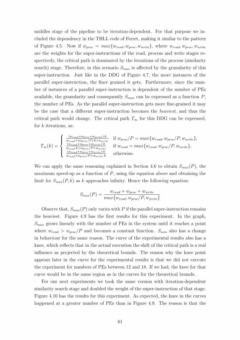
middles stage of the pipeline to be iteration-dependent. For that purpose we in-

cluded the dependency in the THLL code of Ferret, making it similar to the pattern

of Figure 4.5. Now if wproc = max{wread, wproc, wwrite}, where wread, wproc, wwrite

are the weights for the super-instructions of the read, process and write stages re-

spectively, the critical path is dominated by the iterations of the process (similarity

search) stage. Therefore, in this scenario Smax is affected by the granularity of this

super-instruction. Just like in the DDG of Figure 4.7, the more instances of the

parallel super-instruction, the finer grained it gets. Furthermore, since the num-

ber of instances of a parallel super-instruction is dependent of the number of PEs

available, the granularity and consequently Smax can be expressed as a function P ,

the number of PEs. As the parallel super-instruction gets more fine-grained it may

be the case that a different super-instruction becomes the heaviest, and thus the

critical path would change. The critical path T∞ for this DDG can be expressed,

for k iterations, as:

T∞(k) =

(wread+wproc+wwrite)·k

wread+(wproc/P )·k+wwriteif wproc/P = max{wread, wproc/P,wwrite},

(wread+wproc+wwrite)·kwread·k+wproc/P+wwrite

if wread = max{wread, wproc/P,wwrite},(wread+wproc+wwrite)·kwread+wproc/P+wwrite·k otherwise.

We can apply the same reasoning explained in Section 4.6 to obtain Smax(P ), the

maximum speed-up as a function of P , using the equation above and obtaining the

limit for Smax(P, k) as k approaches infinity. Hence the following equation:

Smax(P ) =wread + wproc + wwrite

max{wread, wproc/P,wwrite}

Observe that, Smax(P ) only varies with P if the parallel super-instruction remains

the heaviest. Figure 4.9 has the first results for this experiment. In the graph,

Smax grows linearly with the number of PEs in the system until it reaches a point

where wread > wproc/P and becomes a constant function. Smin also has a change

in behaviour for the same reason. The curve of the experimental results also has a

knee, which reflects that in the actual execution the shift of the critical path is a real

influence as projected by the theoretical bounds. The reason why the knee point

appears later in the curve for the experimental results is that we did not execute

the experiment for numbers of PEs between 12 and 18. If we had, the knee for that

curve would be in the same region as in the curves for the theoretical bounds.

For our next experiments we took the same version with iteration-dependent

similarity search stage and doubled the weight of the super-instruction of that stage.

Figure 4.10 has the results for this experiment. As expected, the knee in the curves

happened at a greater number of PEs than in Figure 4.9. The reason is that the

61

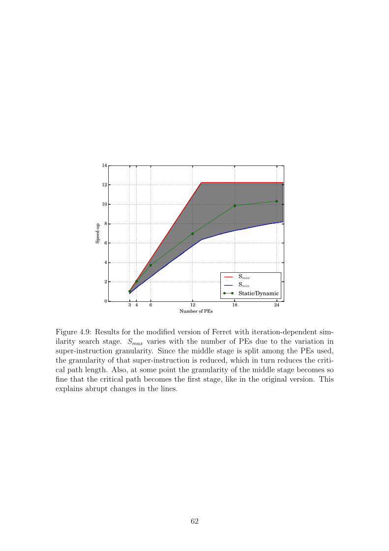
3 4 6 12 18 24Number of PEs

0

2

4

6

8

10

12

14

Spee

d-up

SmaxSminStatic/Dynamic

Figure 4.9: Results for the modified version of Ferret with iteration-dependent sim-ilarity search stage. Smax varies with the number of PEs due to the variation insuper-instruction granularity. Since the middle stage is split among the PEs used,the granularity of that super-instruction is reduced, which in turn reduces the criti-cal path length. Also, at some point the granularity of the middle stage becomes sofine that the critical path becomes the first stage, like in the original version. Thisexplains abrupt changes in the lines.

62

3 4 6 12 18 24Number of PEs

0

5

10

15

20

Spee

d-up

SmaxSminStatic/Dynamic

Figure 4.10: Results for the modified version of Ferret with iteration-dependentsimilarity search stage. Smax varies with the number of PEs due to the variation insuper-instruction granularity. Since the middle stage is split among the PEs used,the granularity of that super-instruction is reduced, which in turn reduces the criticalpath length. Also, at some point the granularity of the middle stage becomes sofine that the critical path becomes the first stage, like in the original version. Thisexplains abrupt changes in the lines.

granularity of the similarity search stage has to be split into more parallel instances

than previously in order for the critical path to switch.

4.8 Eliminating the Restrictions of DDGs

As mentioned in Section 4.1, the restrictions imposed to DDGs may be eliminated

in order to make the model generic, allowing it to represent any dataflow programs.

The reason we chose not to relax the restrictions in this work was to ease the

formalization of the model and the related proofs. In this section, however, we will

introduce how each of the three restrictions can be eliminated, although we will not

provide any formal proof for the strategies adopted.

The first restriction has to do with conditional execution. In order to allow

DDGs to have conditional execution, just like any dataflow graph in TALM, we will

have to take into consideration each possible execution path when calculating T1

and T∞ for the DDG. Basically, if the critical path T∞ and the total work done T1

both depend on the boolean control expressions evaluated during execution (i.e. the

63

equivalent of the branches taken/not taken in Von Neumann execution). We can

devise a work around for this issue by calculating the probability for each boolean

expression to be true (according to profile runs of the program). This probabilities

would be used to calculate the probability of each instruction to be executed, just

like what we did in Algorithm 3.1, and with those probabilities we would be able

to calculate E(T1) and E(T∞). These two expected values would in turn allow us

to calculate the expected values E(Smax) and E(Smin). To calculate the expected

Cmax we can adopt the same strategy at each iteration k of Algorithm 4.1, obtaining

E(Ck) at each step.

The second and the third restrictions can both be addressed by allowing edges

to skip iterations in the unrolling process. This would allow an edge to go from

a instruction in iteration i to target an instruction in iteration i + n, n > 1. The

termination criteria of Algorithm 4.1 would, in this case, have to be altered to

guarantee that all edges that skip iterations would appear in the unrolling process.

This issue can be understood by considering the case of nested loops. The unrolling

process could exercise the inner loop and meet the stop criteria for the algorithm,

but it can be the case that two iterations of the outer loop are independent, and

therefore the algorithm in its original form would fail to examine the concurrency

in its entirety.

64

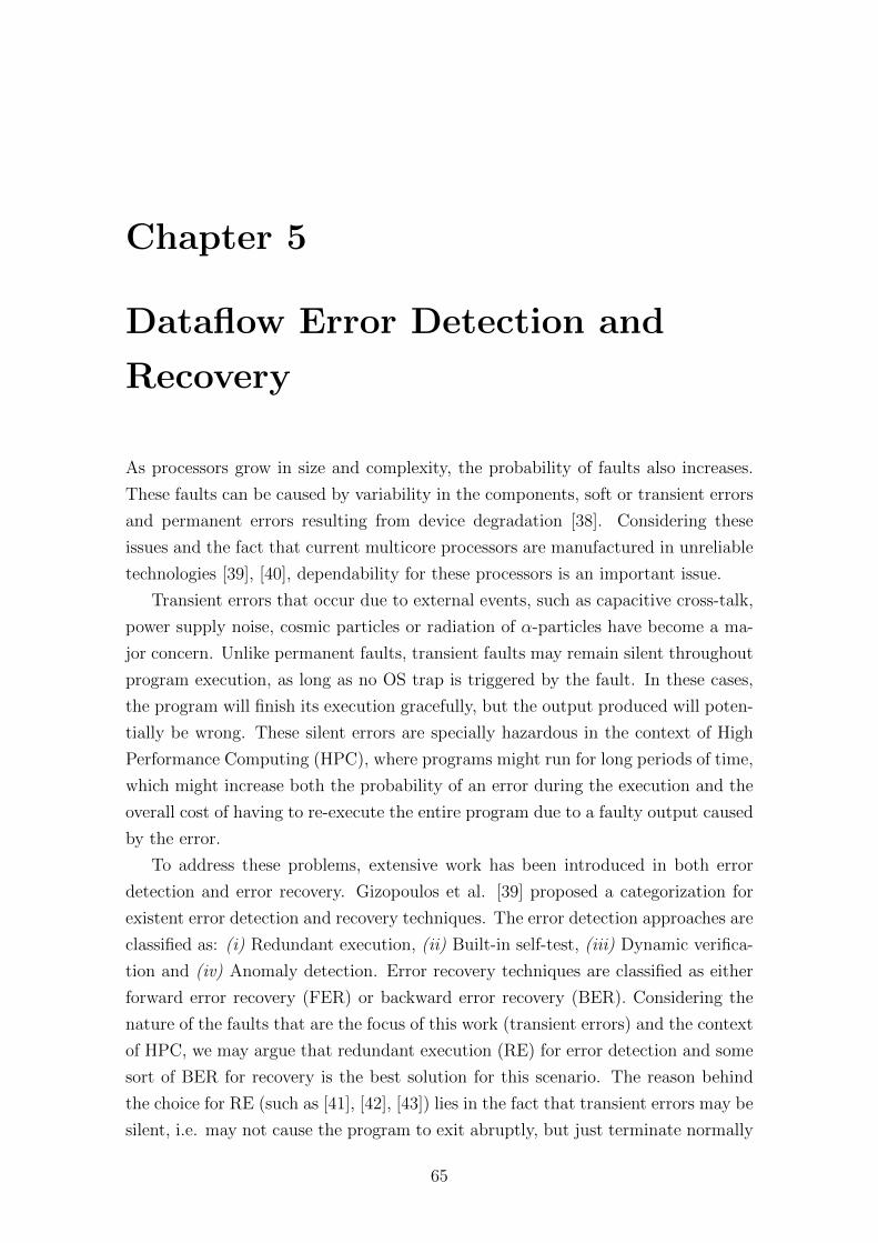
Chapter 5

Dataflow Error Detection and

Recovery

As processors grow in size and complexity, the probability of faults also increases.

These faults can be caused by variability in the components, soft or transient errors

and permanent errors resulting from device degradation [38]. Considering these

issues and the fact that current multicore processors are manufactured in unreliable

technologies [39], [40], dependability for these processors is an important issue.

Transient errors that occur due to external events, such as capacitive cross-talk,

power supply noise, cosmic particles or radiation of α-particles have become a ma-

jor concern. Unlike permanent faults, transient faults may remain silent throughout

program execution, as long as no OS trap is triggered by the fault. In these cases,

the program will finish its execution gracefully, but the output produced will poten-

tially be wrong. These silent errors are specially hazardous in the context of High

Performance Computing (HPC), where programs might run for long periods of time,

which might increase both the probability of an error during the execution and the

overall cost of having to re-execute the entire program due to a faulty output caused

by the error.

To address these problems, extensive work has been introduced in both error

detection and error recovery. Gizopoulos et al. [39] proposed a categorization for

existent error detection and recovery techniques. The error detection approaches are

classified as: (i) Redundant execution, (ii) Built-in self-test, (iii) Dynamic verifica-

tion and (iv) Anomaly detection. Error recovery techniques are classified as either

forward error recovery (FER) or backward error recovery (BER). Considering the

nature of the faults that are the focus of this work (transient errors) and the context

of HPC, we may argue that redundant execution (RE) for error detection and some

sort of BER for recovery is the best solution for this scenario. The reason behind

the choice for RE (such as [41], [42], [43]) lies in the fact that transient errors may be

silent, i.e. may not cause the program to exit abruptly, but just terminate normally

65

while producing a wrong output. If this is the case, the other approaches for error

detection might not notice the silent fault. BER [44], [45], [46], [47] is chosen simply

because the error-free execution tends to have better performance than FER while

consuming less resources, since BER can be implemented with just dual redundancy

and the error detection is off the critical path. Prior work on RE and BER incur in

some important shortcomings such as:

1. The information that has to be stored to create a Recovery Point (RP) com-

prises more than just program data. The architectural state of the processor

is also saved.

2. Checkpointing may involve (and require synchronization with) cores whose

assigned tasks are independent of the ones assigned to the core that is saving

the checkpoint.

3. The interval between checkpoints is not flexible (usually just one interval size

for the entire program) and considers the total sequential work done by a core,

not the data dependencies between portions of the code.

4. A re-execution due to a rollback to a certain Recovery Point will trigger the

re-execution of all the instructions after that RP, even if they are independent

from the faulty data.

5. The communication with the outside world [48] has to wait until a checkpoint

(which may check much more than what is being communicated), instead of

just waiting for the data being sent to be confirmed as error-free. This not

only postpones the output but also may limit the possibility for the overlap of

I/O and computation.

6. Additional hardware is necessary to rollback execution to a RP, making a

software only implementation of these approaches not feasible.

In this chapter we present Dataflow Error Recovery (DFER), a novel mechanism

for online error detection and recovery based on dataflow execution that addresses

the above issues. We argue that dataflow execution is a good fit since it inherently

exposes parallelism in the applications (e.g. [4, 5, 49–55]) and may serve as the basis

for the implementation of an error detection/recovery mechanism that is completely

distributed.

The rest of the chapter is organized as follows: (i) Section 5.1 describes our

proposed approach for error detection/recovery; (ii) Section 5.2 briefly presents our

benchmark set; (iii) Section 5.3 presents the performance results obtained with a

software-only implementation of our approach and (iv) Section 5.4 discusses related

work.

66

5.1 Dataflow Error Detection and Recovery

5.1.1 Error Detection

The basic idea behind our mechanism lies in the addition of tasks responsible for

error detection/recovery to the original dataflow graph. For each task in which error

detection is desired a redundant instance is inserted in the graph and both instances

(we shall refer to them as primary and secondary) will have an outgoing edge to a

third task (called Commit) responsible for the error detection. Both instances will

use this edge to send a message to the Commit task that has the following fields:

1. The unique id of the instance.

2. The input data (operands) the instance consumed for its execution.

3. The unique id of the processing element (PE) to which the instance was

mapped.

4. The data produced by the instance.

Upon receiving that message from both instances of the replicated task, the

Commit task compares the data produced by the primary and the secondary exe-

cutions and, in case a discrepancy is found, a re-execution of the primary instance

is fired. The mechanism for error recovery via re-execution is explained in Section

5.1.4. In order to reduce the amount of data that a Commit task has to compare

(and, therefore, read from main memory) the primary and secondary tasks may send

checksum signatures of the data instead of the data itself. This strategy creates the

possibility of an error remaining undetected, but the probability for that is very

small [56].

5.1.2 Error Recovery

To trigger a re-execution it suffices for the Commit to just send a message to the

PE of the primary task containing the unique id of the task and the input data.

That PE will then re-execute the task at the next idle slot producing a new version

of its output operands (including the message for the Commit). Notice that no

architectural state needs to be saved in order to recover from an error, just the data

consumed by an execution of the task. It is clear, though, that in cases where the

memory region containing the input data is overwritten by the task’s execution, a

mechanism to rollback the memory needs to be applied. This is achieved by logging

the stores made during task execution.

One important aspect of error recovery in dataflow execution is that a re-

execution caused by an error can trigger an entire chain of re-executions of tasks in

67

the graph that depend on the task where the error was detected. As a consequence

of that effect, an error might cause the re-execution of the entire program (in the

worst case scenario). Observe that even though the re-executions caused by an error

may be numerous, in the average case they are still fewer than the re-executions in

previous BER work, since in those approaches all of the work done in the processor

after the recovery point (RP) must be re-executed, not only the work that consumed

faulty data.

Another problem the model has to deal with that is also related to the dependen-

cies between tasks is that it is necessary to verify that the data consumed by each

task is error-free. If a task A produce data with errors and this data is consumed by

a task B, the Commit task responsible for checking B ’s execution should be aware

that the first execution of B was triggered by a faulty execution of A and wait for

the new execution of B, caused by the re-execution of A. The way our mechanism

addresses these problems is presented in Section 5.1.5

5.1.3 Output-Commit Problem

In an error recovery mechanism, it is important to take special care when communi-

cating with the “outside world” [48], i.e. I/O operations. Typically, one will want to

make sure the data being sent to an I/O device is error-free before sending it, since

it may not be so simple (or even impossible) to rollback an I/O operation, so they

have to be placed outside of the sphere of replication [57]. This is referred to as the

output-commmit problem [58] and the way our mechanism addresses this issue is

quite straightforward. To ensure that data consumed by a task is error-free before

it starts executing, it is only necessary to add an edge from the Commit task that

will check that data for the task that will perform the I/O operation. The Commit

task will then be responsible for forwarding the data, which will happen only after

it has been checked and confirmed as error free.

One key advantage of our approach is that this simple solution can be applied to

any kind of I/O operation without the need for special drivers for each device, as is

the case in [58]. So the same solution is used for both network and disk operations,

all that is needed is to enclose the I/O operations in a separate task and have the

data forwarded to it via an edge coming from the Commit task.

5.1.4 Domino Effect Protection

As explained in Section , a re-execution due to an error may cause a whole chain

of re-executions (or domino effect) of the tasks that are dependent on the one in

which the error was detected. In certain programs it may be desirable to avoid the

possibility of a domino effect for the sake of performance. This situation is addressed

68

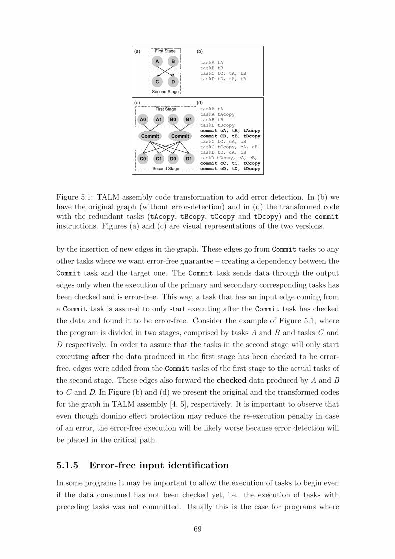
Figure 5.1: TALM assembly code transformation to add error detection. In (b) wehave the original graph (without error-detection) and in (d) the transformed codewith the redundant tasks (tAcopy, tBcopy, tCcopy and tDcopy) and the commit

instructions. Figures (a) and (c) are visual representations of the two versions.

by the insertion of new edges in the graph. These edges go from Commit tasks to any

other tasks where we want error-free guarantee – creating a dependency between the

Commit task and the target one. The Commit task sends data through the output

edges only when the execution of the primary and secondary corresponding tasks has

been checked and is error-free. This way, a task that has an input edge coming from

a Commit task is assured to only start executing after the Commit task has checked

the data and found it to be error-free. Consider the example of Figure 5.1, where

the program is divided in two stages, comprised by tasks A and B and tasks C and

D respectively. In order to assure that the tasks in the second stage will only start

executing after the data produced in the first stage has been checked to be error-

free, edges were added from the Commit tasks of the first stage to the actual tasks of

the second stage. These edges also forward the checked data produced by A and B

to C and D. In Figure (b) and (d) we present the original and the transformed codes

for the graph in TALM assembly [4, 5], respectively. It is important to observe that

even though domino effect protection may reduce the re-execution penalty in case

of an error, the error-free execution will be likely worse because error detection will

be placed in the critical path.

5.1.5 Error-free input identification

In some programs it may be important to allow the execution of tasks to begin even

if the data consumed has not been checked yet, i.e. the execution of tasks with

preceding tasks was not committed. Usually this is the case for programs where

69

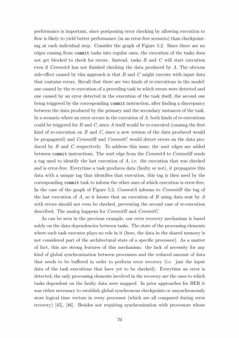
performance is important, since postponing error checking by allowing execution to

flow is likely to yield better performance (in an error-free scenario) than checkpoint-

ing at each individual step. Consider the graph of Figure 5.2. Since there are no

edges coming from commit tasks into regular ones, the execution of the tasks does

not get blocked to check for errors. Instead, tasks B and C will start execution

even if CommitA has not finished checking the data produced by A. The obvious

side-effect caused by this approach is that B and C might execute with input data

that contains errors. Recall that there are two kinds of re-executions in the model:

one caused by the re-execution of a preceding task in which errors were detected and

one caused by an error detected in the execution of the task itself, the second one

being triggered by the corresponding commit instruction, after finding a discrepancy

between the data produced by the primary and the secondary instances of the task.

In a scenario where an error occurs in the execution of A, both kinds of re-executions

could be triggered for B and C, since A itself would be re-executed (causing the first

kind of re-execution on B and C, since a new version of the data produced would

be propagated) and CommitB and CommitC would detect errors on the data pro-

duced by B and C respectively. To address this issue, the wait edges are added

between commit instructions. The wait edge from the CommitA to CommitB sends

a tag used to identify the last execution of A, i.e. the execution that was checked

and is error-free. Everytime a task produces data (faulty or not), it propagates this

data with a unique tag that identifies that execution, this tag is then used by the

corresponding commit task to inform the other ones of which execution is error-free.

In the case of the graph of Figure 5.2, CommitA informs to CommitB the tag of

the last execution of A, so it knows that an execution of B using data sent by A

with errors should not even be checked, preventing the second case of re-execution

described. The analog happens for CommitB and CommitC.

As can be seen in the previous example, our error recovery mechanism is based

solely on the data dependencies between tasks. The state of the processing elements

where each task executes plays no role in it (here, the data in the shared memory is

not considered part of the architectural state of a specific processor). As a matter

of fact, this are strong features of this mechanism: the lack of necessity for any

kind of global synchronization between processors and the reduced amount of data

that needs to be buffered in order to perform error recovery (i.e. just the input

data of the task executions that have yet to be checked). Everytime an error is

detected, the only processing elements involved in the recovery are the ones to which

tasks dependent on the faulty data were mapped. In prior approaches for BER it

was either necessary to establish global synchronous checkpoints or assynchronously

store logical time vectors in every processor (which are all compared during error

recovery) [45], [46]. Besides not requiring synchronization with processors whose

70

A

B

CommitA

C

CommitB

CommitC

w

w

Figure 5.2: Example where wait edges (labeled with w) are necessary to preventunnecessary re-executions. The redundant tasks are omitted for readability, butthere are implicit replications of A, B and C.

tasks are indepdendent of the faulty data, the recovery mechanism also only re-

executes the specific tasks that used faulty data (prior approaches re-execute all the

work in between checkpoints).

5.2 Benchmarks

5.2.1 Longest Common Subsequence (LCS)

This benchmark finds the length of a Longest Common Subsequence (LCS) between

two given sequences using dynamic programming. For two sequences A and B of

length lA and lB, respectively, the application fills up a score matrix (with A ×B elements). LCS consumes a huge amount of memory, which makes is a good

candidate to test the overheads of commit instructions and the effects on scalability

caused by high pressure on the memory bus.

5.2.2 Matrices Multiplication (MxM)

This application reads N square matrices (with the same size) M1,M2, ...,MN and

calculates RN = M1 ×M2 × ... ×MN . It follows an asynchronous pipeline pattern

with 3 stages: Read, Multiply, Free. In each iteration X, the Read stage reads a

new matrix MX , the Multiply stage performs RX = RX−1×MX (in parallel), while

Free deallocates MX and RX−1. It explores data parallelism in the multiplication

stage and overlaps I/O and computation with pipelined execution.

5.2.3 Raytracing (RT)

Renders a scene composed of several spheres that vary on radius, position, trans-

parency and reflexivity. It is a highly scalable application and it performs lots of

computation in a relatively small memory region. In highly scalable CPU bound

applications like RT, reserving half the resources for redundant execution has a big

71

impact, since processors are not idle to be used to execute redundant code. On the

other hand, error detection overheads are expected to be much lower.

5.3 Performance Results

In order to evaluate our mechanism, we implemented DFER in Trebuchet [4], a

software runtime that provides dataflow execution on multicore machines. Because

of the flexibility of the model, a software-only approach can be obtained by adding

the mechanism to any dynamic dataflow runtime, like Trebuchet. Since every aspect

of DFER is based on mere addition of new tasks and edges to the dataflow graph,

it would also be possible to have a hardware implementation on top of a generic

dataflow processor. We ran the benchmarks described in Section 5.2 on a machine

with four AMD Opteron Six-Core chips and 128GB of RAM using our version of

Trebuchet with DFER implemented. Figure 5.3 shows the results for Mxm and

Raytracing while Figure 5.4 shows the results for the LCS benchmark.

It is clear upon observation of the results of the first two benchmarks that over-

heads remain low on applications whose execution do not stress too much the mem-

ory. Both benchmarks presented a huge increase in the overhead of error detec-

tion/recovery in the shift from 6 to 12 primary threads (which are replicated over

12 and 24 cores, respectively). This effect is due to contention in the memory

bandwidth, since the internal operations done in Trebuchet, including our DFER

operations, are done in shared memory and both primary and redundant instances

utilize the same shared memory bandwidth. This is the same effect observed by

Shye et al. in [59].

5.4 Comparison with Prior Work

There exists extensive work on the detection and recovery for transient errors. Unlike

our approach, the absolute majority of prior mechanisms relies on the addition of

specialized hardware to preexisting architectures [39], [44], [46], [57], [60]. AR-SMT

[47] was the first proposed approach for redundant multithreading in SMT cores.

The active and the redundant threads (A and R, respectively) execute in parallel.

Similar to our model, in AR-SMT the primary execution can keep moving forward

even if the redundant execution (also responsible for detection/recovery) lags behind.

This decision is important to achieve good error-free performance.

Error recovery in parallel execution poses extra challenges since when a processor

rolls back to a recovery point it may leave the rest of the system in an inconsistent

state [44] and different approaches have been proposed to address this issue. ReVive

[46] does global checkpointing, synchronizing all processors during checkpoint cre-

72

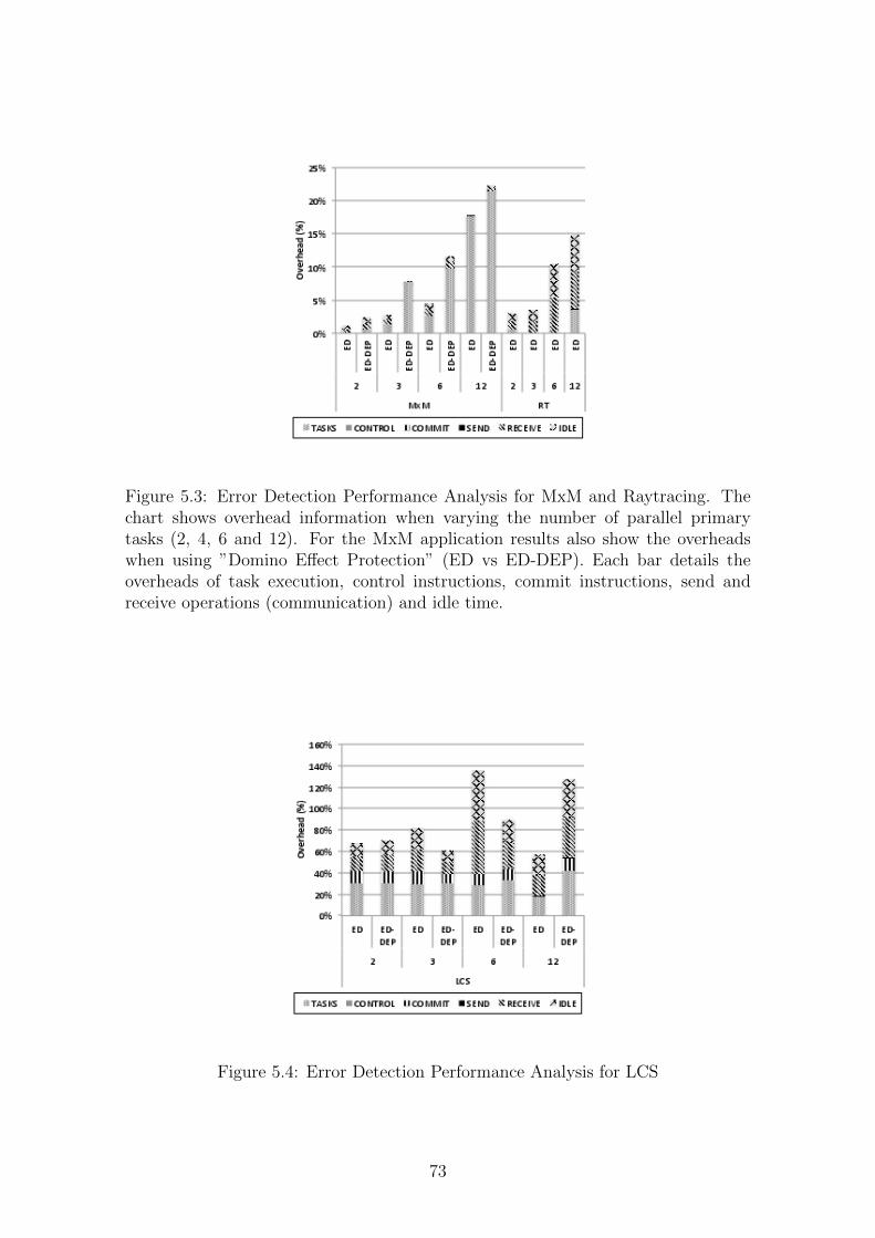
Figure 5.3: Error Detection Performance Analysis for MxM and Raytracing. Thechart shows overhead information when varying the number of parallel primarytasks (2, 4, 6 and 12). For the MxM application results also show the overheadswhen using ”Domino Effect Protection” (ED vs ED-DEP). Each bar details theoverheads of task execution, control instructions, commit instructions, send andreceive operations (communication) and idle time.

Figure 5.4: Error Detection Performance Analysis for LCS

73

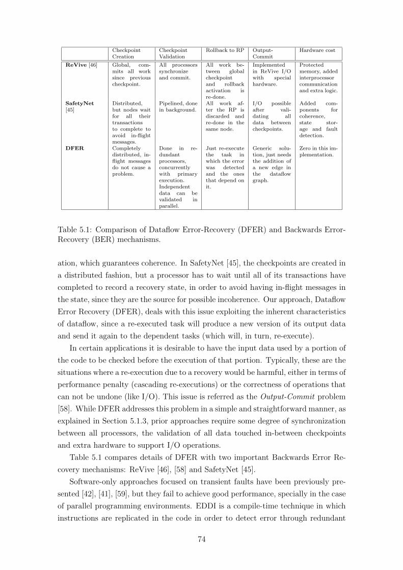
CheckpointCreation

CheckpointValidation

Rollback to RP Output-Commit

Hardware cost

ReVive [46] Global, com-mits all worksince previouscheckpoint.

All processorssynchronizeand commit.

All work be-tween globalcheckpointand rollbackactivation isre-done.

Implementedin ReVive I/Owith specialhardware.

Protectedmemory, addedinterprocessorcommunicationand extra logic.

SafetyNet[45]

Distributed,but nodes waitfor all theirtransactionsto complete toavoid in-flightmessages.

Pipelined, donein background.

All work af-ter the RP isdiscarded andre-done in thesame node.

I/O possibleafter vali-dating alldata betweencheckpoints.

Added com-ponents forcoherence,state stor-age and faultdetection.

DFER Completelydistributed, in-flight messagesdo not cause aproblem.

Done in re-dundantprocessors,concurrentlywith primaryexecution.Independentdata can bevalidated inparallel.

Just re-executethe task inwhich the errorwas detectedand the onesthat depend onit.

Generic solu-tion, just needsthe addition ofa new edge inthe dataflowgraph.

Zero in this im-plementation.

Table 5.1: Comparison of Dataflow Error-Recovery (DFER) and Backwards Error-Recovery (BER) mechanisms.

ation, which guarantees coherence. In SafetyNet [45], the checkpoints are created in

a distributed fashion, but a processor has to wait until all of its transactions have

completed to record a recovery state, in order to avoid having in-flight messages in

the state, since they are the source for possible incoherence. Our approach, Dataflow

Error Recovery (DFER), deals with this issue exploiting the inherent characteristics

of dataflow, since a re-executed task will produce a new version of its output data

and send it again to the dependent tasks (which will, in turn, re-execute).

In certain applications it is desirable to have the input data used by a portion of

the code to be checked before the execution of that portion. Typically, these are the

situations where a re-execution due to a recovery would be harmful, either in terms of

performance penalty (cascading re-executions) or the correctness of operations that

can not be undone (like I/O). This issue is referred as the Output-Commit problem

[58]. While DFER addresses this problem in a simple and straightforward manner, as

explained in Section 5.1.3, prior approaches require some degree of synchronization

between all processors, the validation of all data touched in-between checkpoints

and extra hardware to support I/O operations.

Table 5.1 compares details of DFER with two important Backwards Error Re-

covery mechanisms: ReVive [46], [58] and SafetyNet [45].

Software-only approaches focused on transient faults have been previously pre-

sented [42], [41], [59], but they fail to achieve good performance, specially in the case

of parallel programming environments. EDDI is a compile-time technique in which

instructions are replicated in the code in order to detect error through redundant

74

execution. SWIFT [41] is an extension of EDDI which incorporates control-flow

checking. Both systems incur in huge performance penalty, since the redundancy

is included in the critical path, and do not really treat the issues that arise from

parallel programming.

PLR [59] is another software approach that targets transient faults, by replicating

the entire OS process of the application. Like our implementation, their work relies

on multicores to have the redundancy (a twin process in their case) running in

parallel. However, PLR only works for single-threaded applications and presents

immense overhead (41.1% average) for fault recovery.

75

Chapter 6

Support for GPUs

Most computers available in the market at the moment have at least one GPU,

which is a clear evidence of GPUs’ widespread adoption. The CUDA language [61]

can be considered the standard for GPU programming, since it usually provides

better performance than OpenCL [62]. However, just using CUDA is far from being

sufficient to program applications that use multiple GPUs or that combine CPU and

GPU executions. In such applications it is necessary to orchestrate the execution

in the different computational resources (GPUs and CPUs) in order to establish the

synchronization and the exchange of data between the.

Typically, the programmer will have to implement architecture specific code for

CPU-GPU and GPU-GPU communications, so additional efforts besides the CUDA

programming are needed. Writing this extra code manually may be a difficult task

and can also lead to suboptimal performance depending on the degree of exper-

tise of the programmer. It is very important that the code that coordanates the

computation resources takes advantage of all the overlapping that can be done in

computation and communication. Therefore, it is important to have an abstract

programming model that glues everything together, relieving that burden on the

programmer.

Dataflow has been shown to be a good fit for this task [3, 63, 64], but all previous

work introduces models of dataflow computation that are not as flexible as TALM.

Taking this considerarion we added new functionalities to TALM in order to obtain

GPU capability in our toolchain. We believe that incorporating GPU programming

in our model is a better choice than developing from scratch a new set of tools, since

the new functionalities add no extra overhead to standard TALM execution and this

approach will give us a complete solution for both worlds.

The way we added the support for GPU’s is coherent with the rest of our work,

we included new instructions related to GPU execution to the default instruction

set and instantiate them in dataflow graphs along with the pre-existing instructions.

We also had to introduce the concept of asynchronous operands, in order to support

76

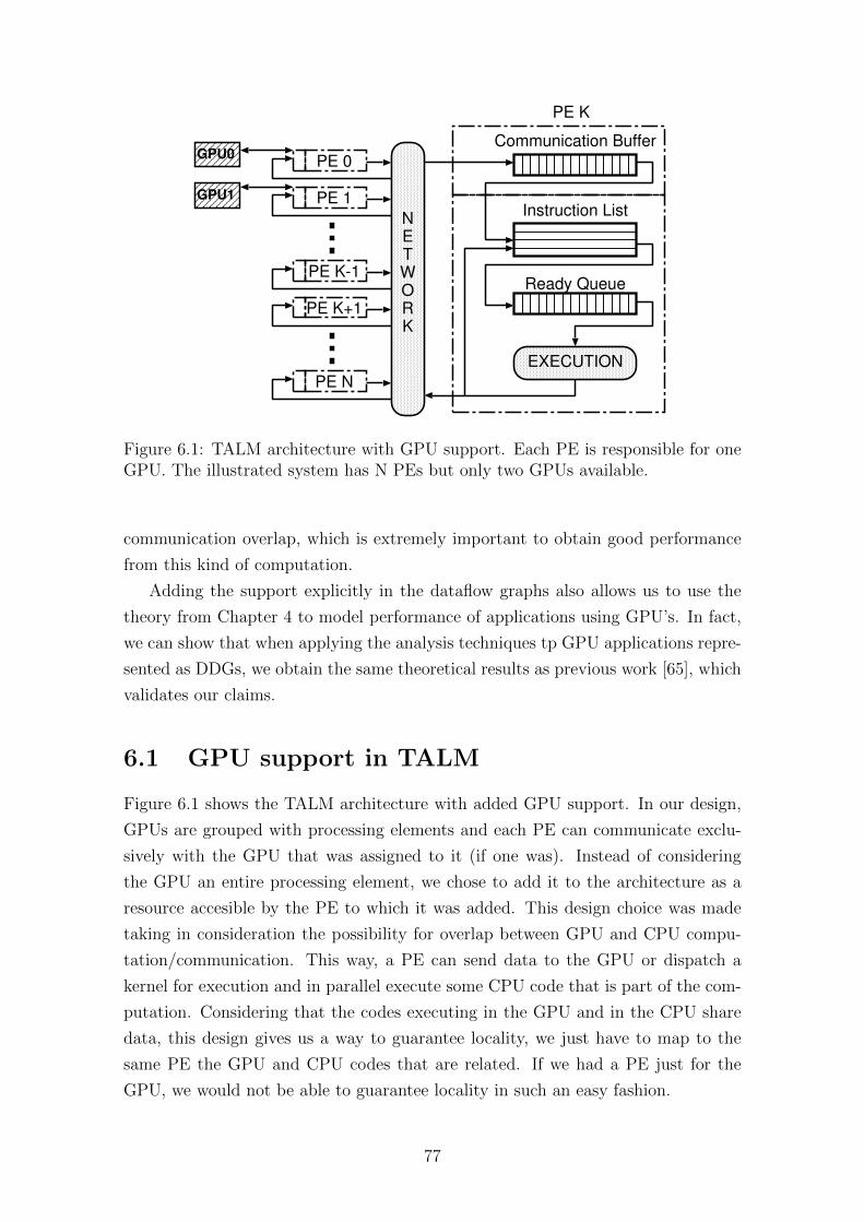
EXECUTION

PE 0

PE K

NETWORK

Communication Buffer

Instruction List

Ready Queue

PE 1

PE K-1

PE K+1

PE N

GPU0

GPU1

Figure 6.1: TALM architecture with GPU support. Each PE is responsible for oneGPU. The illustrated system has N PEs but only two GPUs available.

communication overlap, which is extremely important to obtain good performance

from this kind of computation.

Adding the support explicitly in the dataflow graphs also allows us to use the

theory from Chapter 4 to model performance of applications using GPU’s. In fact,

we can show that when applying the analysis techniques tp GPU applications repre-

sented as DDGs, we obtain the same theoretical results as previous work [65], which

validates our claims.

6.1 GPU support in TALM

Figure 6.1 shows the TALM architecture with added GPU support. In our design,

GPUs are grouped with processing elements and each PE can communicate exclu-

sively with the GPU that was assigned to it (if one was). Instead of considering

the GPU an entire processing element, we chose to add it to the architecture as a

resource accesible by the PE to which it was added. This design choice was made

taking in consideration the possibility for overlap between GPU and CPU compu-

tation/communication. This way, a PE can send data to the GPU or dispatch a

kernel for execution and in parallel execute some CPU code that is part of the com-

putation. Considering that the codes executing in the GPU and in the CPU share

data, this design gives us a way to guarantee locality, we just have to map to the

same PE the GPU and CPU codes that are related. If we had a PE just for the

GPU, we would not be able to guarantee locality in such an easy fashion.

77

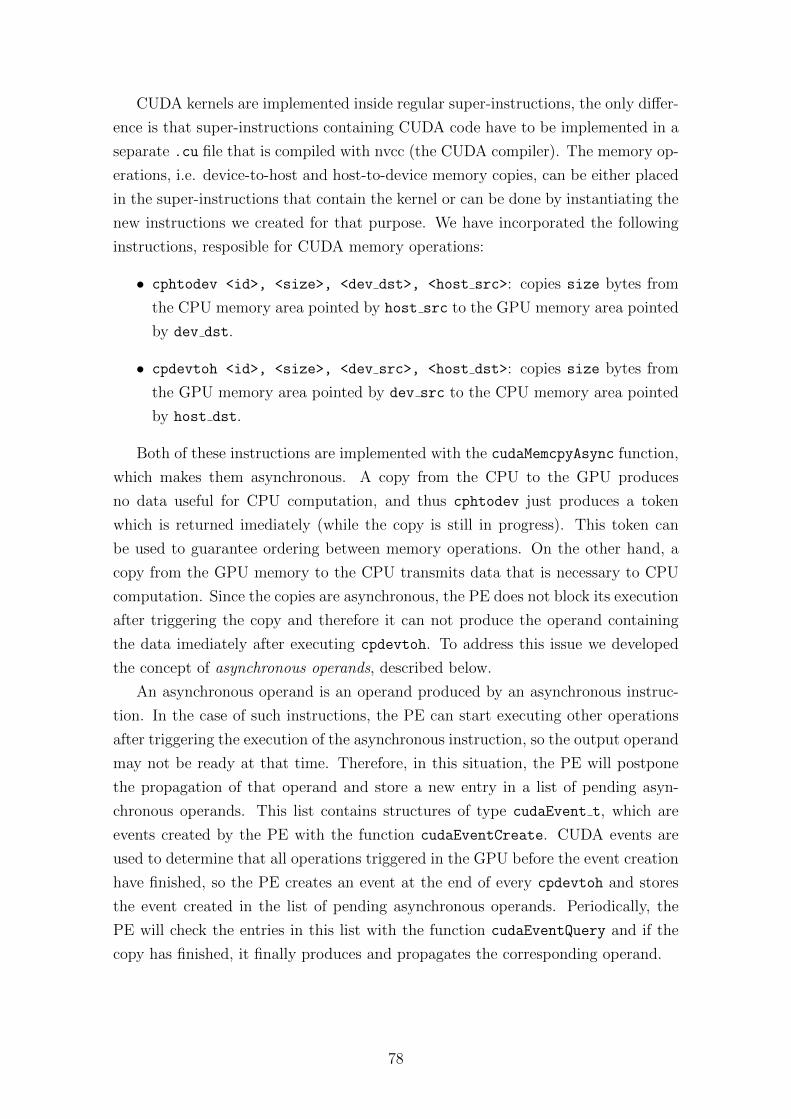
CUDA kernels are implemented inside regular super-instructions, the only differ-

ence is that super-instructions containing CUDA code have to be implemented in a

separate .cu file that is compiled with nvcc (the CUDA compiler). The memory op-

erations, i.e. device-to-host and host-to-device memory copies, can be either placed

in the super-instructions that contain the kernel or can be done by instantiating the

new instructions we created for that purpose. We have incorporated the following

instructions, resposible for CUDA memory operations:

• cphtodev <id>, <size>, <dev dst>, <host src>: copies size bytes from

the CPU memory area pointed by host src to the GPU memory area pointed

by dev dst.

• cpdevtoh <id>, <size>, <dev src>, <host dst>: copies size bytes from

the GPU memory area pointed by dev src to the CPU memory area pointed

by host dst.

Both of these instructions are implemented with the cudaMemcpyAsync function,

which makes them asynchronous. A copy from the CPU to the GPU produces

no data useful for CPU computation, and thus cphtodev just produces a token

which is returned imediately (while the copy is still in progress). This token can

be used to guarantee ordering between memory operations. On the other hand, a

copy from the GPU memory to the CPU transmits data that is necessary to CPU

computation. Since the copies are asynchronous, the PE does not block its execution

after triggering the copy and therefore it can not produce the operand containing

the data imediately after executing cpdevtoh. To address this issue we developed

the concept of asynchronous operands, described below.

An asynchronous operand is an operand produced by an asynchronous instruc-

tion. In the case of such instructions, the PE can start executing other operations

after triggering the execution of the asynchronous instruction, so the output operand

may not be ready at that time. Therefore, in this situation, the PE will postpone

the propagation of that operand and store a new entry in a list of pending asyn-

chronous operands. This list contains structures of type cudaEvent t, which are

events created by the PE with the function cudaEventCreate. CUDA events are

used to determine that all operations triggered in the GPU before the event creation

have finished, so the PE creates an event at the end of every cpdevtoh and stores

the event created in the list of pending asynchronous operands. Periodically, the

PE will check the entries in this list with the function cudaEventQuery and if the

copy has finished, it finally produces and propagates the corresponding operand.

78

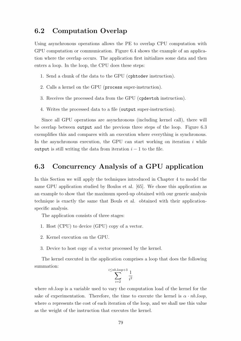
6.2 Computation Overlap

Using asynchronous operations allows the PE to overlap CPU computation with

GPU computation or communication. Figure 6.4 shows the example of an applica-

tion where the overlap occurs. The application first initializes some data and then

enters a loop. In the loop, the CPU does these steps:

1. Send a chunk of the data to the GPU (cphtodev instruction).

2. Calls a kernel on the GPU (process super-instruction).

3. Receives the processed data from the GPU (cpdevtoh instruction).

4. Writes the processed data to a file (output super-instruction).

Since all GPU operations are asynchronous (including kernel call), there will

be overlap between output and the previous three steps of the loop. Figure 6.3

exemplifies this and compares with an execution where everything is synchronous.

In the asynchronous execution, the GPU can start working on iteration i while

output is still writing the data from iteration i− 1 to the file.

6.3 Concurrency Analysis of a GPU application

In this Section we will apply the techniques introduced in Chapter 4 to model the

same GPU application studied by Boulos et al. [65]. We chose this application as

an example to show that the maximum speed-up obtained with our generic analysis

technique is exactly the same that Bouls et al. obtained with their application-

specific analysis.

The application consists of three stages:

1. Host (CPU) to device (GPU) copy of a vector.

2. Kernel execution on the GPU.

3. Device to host copy of a vector processed by the kernel.

The kernel executed in the application comprises a loop that does the following

summation:i≤nb loop+3∑

i=2

1

i2

where nb loop is a variable used to vary the computation load of the kernel for the

sake of experimentation. Therefore, the time to execute the kernel is α · nb loop,where α represents the cost of each iteration of the loop, and we shall use this value

as the weight of the instruction that executes the kernel.

79

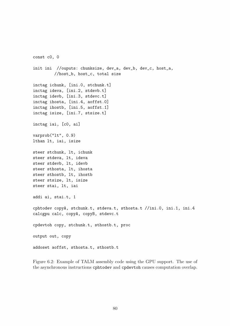
const c0, 0

init ini //ouputs: chunksize, dev_a, dev_b, dev_c, host_a,

//host_b, host_c, total size

inctag ichunk, [ini.0, stchunk.t]

inctag ideva, [ini.2, stdevb.t]

inctag idevb, [ini.3, stdevc.t]

inctag ihosta, [ini.4, aoffst.0]

inctag ihostb, [ini.5, aoffst.1]

inctag isize, [ini.7, stsize.t]

inctag iai, [c0, ai]

varprob("lt", 0.9)

lthan lt, iai, isize

steer stchunk, lt, ichunk

steer stdeva, lt, ideva

steer stdevb, lt, idevb

steer sthosta, lt, ihosta

steer sthostb, lt, ihostb

steer stsize, lt, isize

steer stai, lt, iai

addi ai, stai.t, 1

cphtodev copyA, stchunk.t, stdeva.t, sthosta.t //ini.0, ini.1, ini.4

calcgpu calc, copyA, copyB, stdevc.t

cpdevtoh copy, stchunk.t, sthostb.t, proc

output out, copy

addoset aoffst, sthosta.t, sthostb.t

Figure 6.2: Example of TALM assembly code using the GPU support. The use ofthe asynchronous instructions cphtodev and cpdevtoh causes computation overlap.

80

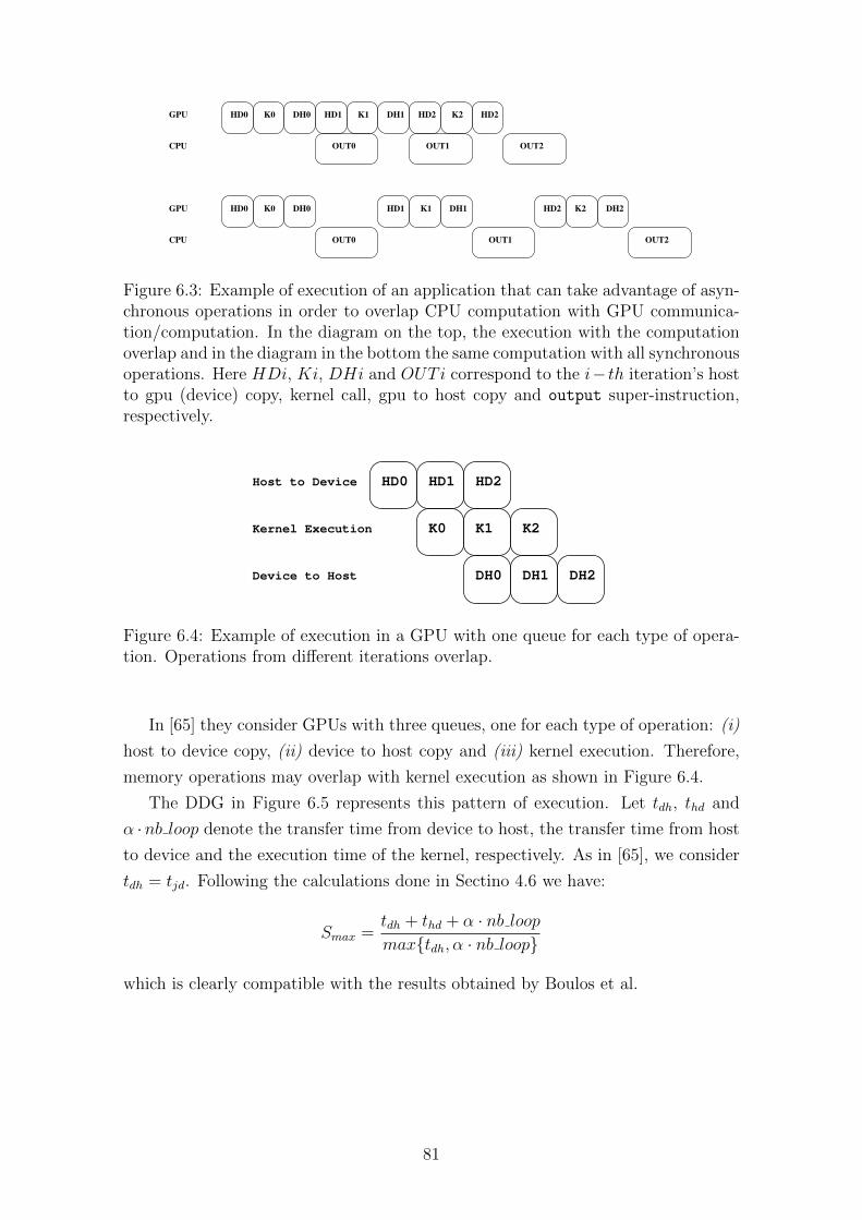
HD0 K0 DH0 HD1 K1 DH1 HD2 K2 HD2

HD0 K0 DH0 HD1 K1 DH1 HD2 K2 DH2

OUT0 OUT1 OUT2

OUT0 OUT1 OUT2

GPU

GPU

CPU

CPU

Figure 6.3: Example of execution of an application that can take advantage of asyn-chronous operations in order to overlap CPU computation with GPU communica-tion/computation. In the diagram on the top, the execution with the computationoverlap and in the diagram in the bottom the same computation with all synchronousoperations. Here HDi, Ki, DHi and OUTi correspond to the i− th iteration’s hostto gpu (device) copy, kernel call, gpu to host copy and output super-instruction,respectively.

HD0 HD1 HD2

K0 K1 K2

DH0 DH1 DH2

Host to Device

Kernel Execution

Device to Host

Figure 6.4: Example of execution in a GPU with one queue for each type of opera-tion. Operations from different iterations overlap.

In [65] they consider GPUs with three queues, one for each type of operation: (i)

host to device copy, (ii) device to host copy and (iii) kernel execution. Therefore,

memory operations may overlap with kernel execution as shown in Figure 6.4.

The DDG in Figure 6.5 represents this pattern of execution. Let tdh, thd and

α ·nb loop denote the transfer time from device to host, the transfer time from host

to device and the execution time of the kernel, respectively. As in [65], we consider

tdh = tjd. Following the calculations done in Sectino 4.6 we have:

Smax =tdh + thd + α · nb loopmax{tdh, α · nb loop}

which is clearly compatible with the results obtained by Boulos et al.

81

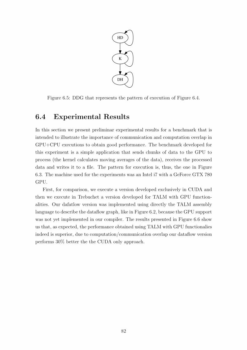
HD

K

DH

Figure 6.5: DDG that represents the pattern of execution of Figure 6.4.

6.4 Experimental Results

In this section we present preliminar experimental results for a benchmark that is

intended to illustrate the importance of communication and computation overlap in

GPU+CPU executions to obtain good performance. The benchmark developed for

this experiment is a simple application that sends chunks of data to the GPU to

process (the kernel calculates moving averages of the data), receives the processed

data and writes it to a file. The pattern for execution is, thus, the one in Figure

6.3. The machine used for the experiments was an Intel i7 with a GeForce GTX 780

GPU.

First, for comparison, we execute a version developed exclusively in CUDA and

then we execute in Trebuchet a version developed for TALM with GPU function-

alities. Our dafatlow version was implemented using directly the TALM assembly

language to describe the dataflow graph, like in Figure 6.2, because the GPU support

was not yet implemented in our compiler. The results presented in Figure 6.6 show

us that, as expected, the performance obtained using TALM with GPU functionalies

indeed is superior, due to computation/communication overlap our dataflow version

performs 30% better the the CUDA only approach.

82

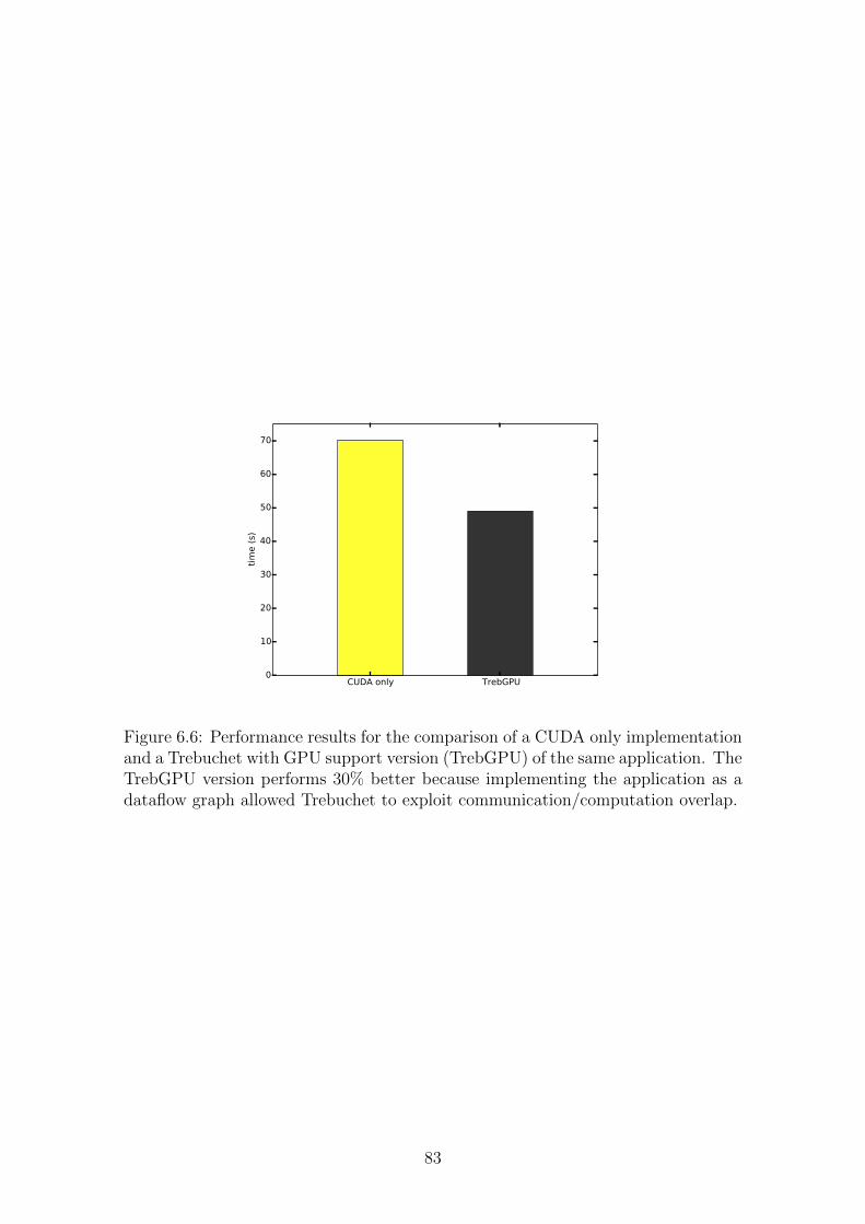
CUDA only TrebGPU0

10

20

30

40

50

60

70

tim

e (

s)

Figure 6.6: Performance results for the comparison of a CUDA only implementationand a Trebuchet with GPU support version (TrebGPU) of the same application. TheTrebGPU version performs 30% better because implementing the application as adataflow graph allowed Trebuchet to exploit communication/computation overlap.

83

Chapter 7

Discussion and Future Work

In this work we presented novel techniques to take advantage of dataflow program-

ming and execution. Although in our experiments we focused on implementing these

techniques to our TALM model, they can be applied to any execution model that

follows the dynamic dataflow principle.

In Chapter 3 we introduced a static scheduling algorithm based on list schedul-

ing that takes into consideration conditional execution, which is an integral part of

dataflow execution. Our Selective Work-Stealing algorithm, presented in the same

chapter, allows the programmer complete flexibility over what work should be stolen.

This was not possible in prior approaches on work-stealing. The algorithm intro-

duced in Acar et al. [10], allows data locality to be exploited, but it adds the need

for extra data structures (the mailboxes) and extra synchronization. Our approach

uses just the traditional deque with a variation on how it is accessed and allows the

programmer to define a heuristic for what work to steal.

In Section 3.9 we studied the case of parallelizing dynamic programming algo-

rithms using dataflow and presented promising results for the case of the algorihtm

that finds a longest common subsequence of two sequences, an important algorithm

in the field of bioinformatics. Our experiments showed an improve in performance

of up to 23% over an implementation using the traditional wavefront method.

The concurrency analysis introduced in Chapter 4 extend prior work that focused

only on DAGs. We presented a definition of Dynamic Dataflow Graphs (DDGs),

which we used as our model of computation for the analysis. This new model of

computation allowed us to abstract details of dataflow implementation, since DDGs

are more simple and easier to analyze than TALM graphs, for instance, and gain

important insight into the behaviour of dataflow parallelization. We showed how

to obtain two important metrics via analysis of DDGs: the maximum speed-up (or

average degree of concurrency) Smax and the maximum degree of concurrency Cmax.

We also were able to present an important result, the fact that the former is bounded

even if the latter is not. Our experiments with a benchmark that represented the

84

streaming parallel programming pattern showed us that our analysis indeed is able

to model and predict the performance behaviour of applications parallelized with

dataflow execution.

Using the techniques for analysis of DDGs we were also able to extend our static

scheduling algorithm to exploit parallelism between different iterations, which was

not taken in consideration in previous approaches. Besides the algorithm itself

there is an important lesson learned with its implementation: all the information

that describes the parallel programming pattern in the program is in the dataflow

graph, i.e. the data dependencies in the program. Therefore, high-level annotations

or templates that specify what programming pattern is adopted are not necessary.

For instance, using our techniques it is not necessary to specify (or use a special

template) that a certain application has a pipeline pattern, the programmer just

has to describe the dependencies and the static scheduling algorithm will be able to

determine to number of PEs to allocate (using Cmax) and how to spread the pipeline

stages among them.

Our Dataflow Error Detection and Recovery (DFER) algorithm was shown to

be a promising option for dealing with transient errors. Our experiments using an

implementation of DFER in the Trebuchet dataflow runtime [4] showed the efficiency

of the mechanism. We observed that error detection overhead is highly related to

the amount of memory accesses performed by the application. Benchmarks that

stress out the memory BUS presented performance deterioration, while for other

benchmarks overheads were up to 23%. The flexibility of the mechanism allowed us

to deal with issues like the output-commit problem in an easy fashion, adding very

little complexity to the application.

The experiments using different numbers of cores also showed us that DFER is

indeed distributed in all of its aspects, as was expected since it is entirely imple-

mented as additions to the dataflow graph of the application, which makes it inher-

ently parallelizable. However, scalability was far from linear in the applications that

were more memory-bound. This issue arose from the contention on memory, since

both primary and redundant executions share the same memory bandwidth. This

kind of overhead was also pointed by the authors of PLR [59], as in PLR primary

and redundant also share memory bandwidth, which corroborates our assumption.

Taking all of this in consideration we believe that DFER is a good mechanism

for error recovery. Although results are already promising in the current implemen-

tation, it is safe to assume the performance in a cluster implementation of the same

dataflow runtime or even a hardware implementation would be even better, since the

memory bandwidth would not impose such a burden on scalability. Also, comparing

the principles of DFER with the characteristis of prior work, we can safely judge

that DFER would be a solid option not only for people already using dataflow, but

85

also for those who are willing to shift paradigms to obtain the advantages of this

completely distributed approach.

In Chapter 6 we introduced the GPU support for TALM. The mechanisms in-

cluding for GPU support are coherent with the rest of our work, we aimed at adding

the functionalities to the dataflow graph itself, taking advantage of its inherent par-

allel nature. We were also able to show that by incorporating GPU operations to

the dataflow graph it is possible to apply the same techniques introduced in Chapter

4 to analyze the concurrency in programs that use GPUs. Although our compiler

does not yet support GPU programming, this feature is the focus of ongoing work

and will be provided in the next version.

The concept of asynchronous operands developed to add the GPU functional-

ity can be applied for asynchronous I/O operations. As a matter of fact, we are

currently working on implementing support to Linux Asynchronous I/O (AIO). Ba-

sically, I/O operations executed in super-instructions, like a write to a file, would

be substituted for Linux AIO operations whose results would become pending asyn-

chronous operands and the PE would regain control immediately after triggering the

operations, being thus able to overlap I/O and computation. This way, there would

be no more need to use thread oversubscription to achieve I/O and computation

overlap in a PE.

86

Bibliography

[1] DURAN, A., AYGUAD, E., BADIA, R. M., et al. “Ompss: a Proposal for Pro-

gramming Heterogeneous Multi-Core Architectures.” Parallel Processing

Letters, v. 21, n. 2, pp. 173–193, 2011. Available at: <http://dblp.

uni-trier.de/db/journals/ppl/ppl21.html#DuranABLMMP11>.

[2] KYRIACOU, C., EVRIPIDOU, P., TRANCOSO, P. “Data-Driven Multi-

threading Using Conventional Microprocessors”, IEEE Transactions

on Parallel and Distributed Systems, v. 17, n. 10, pp. 1176–1188, out.

2006. ISSN: 1045-9219. doi: 10.1109/TPDS.2006.136. Available at:

<http://ieeexplore.ieee.org/xpl/freeabs_all.jsp?arnumber=

1687886http://ieeexplore.ieee.org/lpdocs/epic03/wrapper.htm?

arnumber=1687886>.

[3] GAUTIER, T., LIMA, J. V., MAILLARD, N., et al. “XKaapi: A Runtime

System for Data-Flow Task Programming on Heterogeneous Architec-

tures”, 2013 IEEE 27th International Symposium on Parallel and Dis-

tributed Processing, pp. 1299–1308, maio 2013. doi: 10.1109/IPDPS.2013.

66. Available at: <http://ieeexplore.ieee.org/lpdocs/epic03/

wrapper.htm?arnumber=6569905>.

[4] ALVES, T. A., MARZULO, L. A., FRANCA, F. M., et al. “Trebuchet: ex-

ploring TLP with dataflow virtualisation”, International Journal of High

Performance Systems Architecture, v. 3, n. 2/3, pp. 137, 2011. ISSN:

1751-6528. doi: 10.1504/IJHPSA.2011.040466.

[5] MARZULO, L. A. J., ALVES, T. A., FRANCA, F. M. G., et al. “TALM: A Hy-

brid Execution Model with Distributed Speculation Support”, Computer

Architecture and High Performance Computing Workshops, International

Symposium on, v. 0, pp. 31–36, 2010. doi: 10.1109/SBAC-PADW.2010.8.

[6] FRANKLIN, M. A., TYSON, E. J., BUCKLEY, J., et al. “Auto-Pipe and the X

Language : A Pipeline Design Tool and Description Language Tool and

Description Language ,in Proc. of Intl Parallel and Distributed Auto-Pipe

87

http://dblp.uni-trier.de/db/journals/ppl/ppl21.html#DuranABLMMP11

http://dblp.uni-trier.de/db/journals/ppl/ppl21.html#DuranABLMMP11

http://ieeexplore.ieee.org/xpl/freeabs_all.jsp?arnumber=1687886 http://ieeexplore.ieee.org/lpdocs/epic03/wrapper.htm?arnumber=1687886



http://ieeexplore.ieee.org/lpdocs/epic03/wrapper.htm?arnumber=6569905


and the X Language : A Pipeline Design Tool and Description Language”,

, n. April, 2006.

[7] THIES, W., KARCZMAREK, M., AMARASINGHE, S. “StreamIt: A language

for streaming applications”, Compiler Construction, 2002. Available at:

<http://www.springerlink.com/index/LC5B77HWR8J2UBHK.pdf>.

[8] THIES, W., AMARASINGHE, S. “An empirical characterization of stream pro-

grams and its implications for language and compiler design”, Proceedings

of the 19th international conference on Parallel architectures and compila-

tion techniques - PACT ’10, p. 365, 2010. doi: 10.1145/1854273.1854319.

Available at: <http://portal.acm.org/citation.cfm?doid=1854273.

1854319>.

[9] REINDERS, J. Intel Threading Building Blocks. First ed. Sebastopol, CA, USA,

O’Reilly & Associates, Inc., 2007. ISBN: 9780596514808.

[10] ACAR, U. A., BLELLOCH, G. E., BLUMOFE, R. D. “The Data Locality of

Work Stealing”. In: Proceedings of the Twelfth Annual ACM Symposium

on Parallel Algorithms and Architectures, SPAA ’00, pp. 1–12, New York,

NY, USA, 2000. ACM. ISBN: 1-58113-185-2. doi: 10.1145/341800.341801.

Available at: <http://doi.acm.org/10.1145/341800.341801>.

[11] NAVARRO, A., ASENJO, R., TABIK, S., et al. “Load balancing using work-

stealing for pipeline parallelism in emerging applications”. In: Proceedings

of the 23rd international conference on Supercomputing, ICS ’09, pp. 517–

518, New York, NY, USA, 2009. ACM. ISBN: 978-1-60558-498-0. doi:

10.1145/1542275.1542358.

[12] MERCALDI, M., SWANSON, S., PETERSEN, A., et al. “Modeling instruc-

tion placement on a spatial architecture”. In: SPAA ’06: Proceedings

of the eighteenth annual ACM symposium on Parallelism in algorithms

and architectures, pp. 158–169, New York, NY, USA, 2006. ACM. ISBN:

1-59593-452-9. doi: 10.1145/1148109.1148137.

[13] SWANSON, S., SCHWERIN, A., MERCALDI, M., et al. “The WaveScalar

architecture”, ACM Transactions on Computer Systems, v. 25, n. 2,

pp. 4–es, maio 2007. ISSN: 07342071. doi: 10.1145/1233307.1233308.

[14] SIH, G. C., LEE, E. A. “A Compile-Time Scheduling Heuristic Heterogeneous

Processor Architectures”, v. 4, n. 2, pp. 175–187, 1993.

[15] TOPCUOGLU, H., HARIRI, S., SOCIETY, I. C. “Performance-Effective and

Low-Complexity”, Computer, v. 13, n. 3, pp. 260–274, 2002.

88

http://www.springerlink.com/index/LC5B77HWR8J2UBHK.pdf

http://portal.acm.org/citation.cfm?doid=1854273.1854319

http://portal.acm.org/citation.cfm?doid=1854273.1854319

http://doi.acm.org/10.1145/341800.341801

[16] BOYER, W. F., HURA, G. S. “Non-evolutionary algorithm for schedul-

ing dependent tasks in distributed heterogeneous computing environ-

ments”, Journal of Parallel and Distributed Computing, v. 65, n. 9,

pp. 1035–1046, set. 2005. ISSN: 07437315. doi: 10.1016/j.jpdc.2005.04.

017. Available at: <http://linkinghub.elsevier.com/retrieve/pii/

S0743731505000900>.

[17] ARORA, N. S., BLUMOFE, R. D., PLAXTON, C. G. “Thread Scheduling

for Multiprogrammed Multiprocessors”, Theory of Computing Systems,

v. 34, n. 2, pp. 115–144, jan. 2001. ISSN: 1432-4350. doi: 10.1007/

s002240011004.

[18] BLUMOFE, R. D., JOERG, C. F., KUSZMAUL, B. C., et al. “Cilk: An Ef-

ficient Multithreaded Runtime System”. In: JOURNAL OF PARALLEL

AND DISTRIBUTED COMPUTING, pp. 207–216, 1995.

[19] CHASE, D., LEV, Y. “Dynamic circular work-stealing deque”, Proceedings

of the 17th annual ACM symposium on Parallelism in algorithms and

architectures - SPAA’05, , n. c, pp. 21, 2005. doi: 10.1145/1073970.

1073974.

[20] GUO, Y., ZHAO, J., CAVE, V., et al. “SLAW: A scalable locality-aware

adaptive work-stealing scheduler”, 2010 IEEE International Symposium

on Parallel & Distributed Processing (IPDPS), pp. 1–12, 2010. doi:

10.1109/IPDPS.2010.5470425.

[21] ALVES, T. A. O., MARZULO, L. A. J., FRANCA, F. M. G., et al. “Trebuchet:

Exploring TLP with Dataflow Virtualisation”, Int. J. High Perform. Syst.

Archit., v. 3, n. 2/3, pp. 137–148, maio 2011. ISSN: 1751-6528. doi:

10.1504/IJHPSA.2011.040466. Available at: <http://dx.doi.org/10.

1504/IJHPSA.2011.040466>.

[22] CHANDY, K. M., LAMPORT, L. “Distributed snapshots: determining global

states of distributed systems”, ACM Transactions on Computer Systems,

v. 3, n. 1, pp. 63–75, fev. 1985. ISSN: 07342071. doi: 10.1145/214451.

214456.

[23] CONTRERAS, G., MARTONOSI, M. “Characterizing and improving the

performance of Intel Threading Building Blocks”, 2008 IEEE Interna-

tional Symposium on Workload Characterization, pp. 57–66, out. 2008.

doi: 10.1109/IISWC.2008.4636091. Available at: <http://ieeexplore.

ieee.org/lpdocs/epic03/wrapper.htm?arnumber=4636091>.

89

http://linkinghub.elsevier.com/retrieve/pii/S0743731505000900

http://linkinghub.elsevier.com/retrieve/pii/S0743731505000900

http://dx.doi.org/10.1504/IJHPSA.2011.040466

http://dx.doi.org/10.1504/IJHPSA.2011.040466



[24] MARZULO, L. A. J., ALVES, T. A. O., FRANCA, F. M. G., et al. “Couil-

lard: Parallel Programming via Coarse-Grained Data-Flow Compilation”,

CoRR, v. abs/1109.4925, 2011. Available at: <http://dblp.uni-trier.

de/db/journals/corr/corr1109.html#abs-1109-4925>.

[25] LOMBARDI, M., MILANO, M., RUGGIERO, M., et al. “Stochastic al-

location and scheduling for conditional task graphs in multi-processor

systems-on-chip”, Journal of Scheduling, pp. 315–345, 2010. doi: 10.

1007/s10951-010-0184-y.

[26] HERLIHY, M. “Wait-free Synchronization”, ACM Trans. Program. Lang.

Syst., v. 13, n. 1, pp. 124–149, jan. 1991. ISSN: 0164-0925. doi:

10.1145/114005.102808. Available at: <http://doi.acm.org/10.1145/

114005.102808>.

[27] WAGNER, R. A., FISCHER, M. J. “The String-to-String Correction Problem”,

J. ACM, v. 21, n. 1, pp. 168–173, jan. 1974. ISSN: 0004-5411. doi:

10.1145/321796.321811. Available at: <http://doi.acm.org/10.1145/

321796.321811>.

[28] ALVES, T. A., MARZULO, L. A. J., FRANCA, F. M. G., et al. “Trebuchet:

Explorando TLP com Virtualizacao DataFlow”. In: WSCAD-SSC’09, pp.

60–67, Sao Paulo, out. 2009. SBC.

[29] ANVIK, J., MACDONALD, S., SZAFRON, D., et al. “Generating Parallel

Programs from the Wavefront Design Pattern”. In: Proceedings of the 16th

International Parallel and Distributed Processing Symposium, IPDPS ’02,

pp. 165–, Washington, DC, USA, 2002. IEEE Computer Society. ISBN:

0-7695-1573-8. Available at: <http://dl.acm.org/citation.cfm?id=

645610.661717>.

[30] BLUMOFE, R. D., LEISERSON, C. E. “Scheduling Multithreaded Computa-

tions by Work Stealing 1 Introduction”, pp. 1–29.

[31] EAGER, D., ZAHORJAN, J., LAZOWSKA, E. “Speedup versus effi-

ciency in parallel systems”, IEEE Transactions on Computers, v. 38,

n. 3, pp. 408–423, mar. 1989. ISSN: 00189340. doi: 10.1109/12.



[32] KUMAR, B., GONSALVES, T. A. “Modelling and Analysis of Distributed

Software Systems”. In: Proceedings of the Seventh ACM Symposium on

Operating Systems Principles, SOSP ’79, pp. 2–8, New York, NY, USA,

90

http://dblp.uni-trier.de/db/journals/corr/corr1109.html#abs-1109-4925

http://dblp.uni-trier.de/db/journals/corr/corr1109.html#abs-1109-4925

http://doi.acm.org/10.1145/114005.102808

http://doi.acm.org/10.1145/114005.102808

http://doi.acm.org/10.1145/321796.321811

http://doi.acm.org/10.1145/321796.321811

http://dl.acm.org/citation.cfm?id=645610.661717

http://dl.acm.org/citation.cfm?id=645610.661717



1979. ACM. ISBN: 0-89791-009-5. doi: 10.1145/800215.806563. Available

at: <http://doi.acm.org/10.1145/800215.806563>.

[33] LOMBARDI, M., MILANO, M. “Scheduling Conditional Task Graphs.” In:

Bessiere, C. (Ed.), CP, v. 4741, Lecture Notes in Computer Science, pp.

468–482. Springer, 2007. ISBN: 978-3-540-74969-1. Available at: <http:

//dblp.uni-trier.de/db/conf/cp/cp2007.html#LombardiM07>.

[34] ANTICONA, M. T. “A GRASP algorithm to solve the problem of dependent

tasks scheduling in different machines.” In: Bramer, M. (Ed.), IFIP AI,

v. 217, IFIP, pp. 325–334. Springer, 2006. ISBN: 0-387-34654-6. Avail-

able at: <http://dblp.uni-trier.de/db/conf/ifip12/ai2006.html#

Anticona06>.

[35] AHO, A. V., ULLMAN, J. D. Principles of Compiler Design (Addison-

Wesley Series in Computer Science and Information Processing). Boston,

MA, USA, Addison-Wesley Longman Publishing Co., Inc., 1977. ISBN:

0201000229.

[36] HERLIHY, M., SHAVIT, N. The Art of Multiprocessor Programming. San

Francisco, CA, USA, Morgan Kaufmann Publishers Inc., 2008. ISBN:

0123705916, 9780123705914.

[37] BIENIA, C., KUMAR, S., SINGH, J. P., et al. “The PARSEC Benchmark Suite:

Characterization and Architectural Implications”. In: Proceedings of the

17th International Conference on Parallel Architectures and Compilation

Techniques, PACT ’08, pp. 72–81, New York, NY, USA, 2008. ACM.

ISBN: 978-1-60558-282-5. doi: 10.1145/1454115.1454128. Available at:

<http://doi.acm.org/10.1145/1454115.1454128>.

[38] BORKAR, S. “D ESIGNING R ELIABLE S YSTEMS FROM U NRELIABLE

C OMPONENTS : T HE C HALLENGES OF T RANSISTOR V ARI-

ABILITY AND D EGRADATION”, pp. 10–16, 2005.

[39] GIZOPOULOS, D., PSARAKIS, M., ADVE, S. V., et al. “Architectures

for online error detection and recovery in multicore processors”, 2011

Design, Automation & Test in Europe, , n. c, pp. 1–6, mar. 2011.

doi: 10.1109/DATE.2011.5763096. Available at: <http://ieeexplore.

ieee.org/lpdocs/epic03/wrapper.htm?arnumber=5763096>.

[40] SHIVAKUMAR, P., KISTLER, M., KECKLER, S., et al. “Model-

ing the effect of technology trends on the soft error rate of com-

binational logic”, Proceedings International Conference on Depend-

91

http://doi.acm.org/10.1145/800215.806563

http://dblp.uni-trier.de/db/conf/cp/cp2007.html#LombardiM07

http://dblp.uni-trier.de/db/conf/cp/cp2007.html#LombardiM07

http://dblp.uni-trier.de/db/conf/ifip12/ai2006.html#Anticona06

http://dblp.uni-trier.de/db/conf/ifip12/ai2006.html#Anticona06

http://doi.acm.org/10.1145/1454115.1454128



able Systems and Networks, pp. 389–398, 2002. doi: 10.1109/DSN.

2002.1028924. Available at: <http://ieeexplore.ieee.org/lpdocs/

epic03/wrapper.htm?arnumber=1028924>.

[41] REIS, G., CHANG, J., VACHHARAJANI, N., et al. “SWIFT: Soft-

ware Implemented Fault Tolerance”, International Symposium on Code

Generation and Optimization, pp. 243–254. doi: 10.1109/CGO.2005.



[42] OH, N., SHIRVANI, P. P., MCCLUSKEY, E. J. “Reliable Computing TECH-

NICAL Error Detection by Duplicated Instructions”, , n. 2, 2000.

[43] AGGARWAL, N., JOUPPI, N. P., SMITH, J. E. “Configurable Isolation :

Building High Availability Systems with Commodity Multi-Core Proces-

sors”, 2007.

[44] SORIN, D. J. Fault Tolerant Computer Architecture, v. 4. jan. 2009. ISBN:

9781598299533. doi: 10.2200/S00192ED1V01Y200904CAC005.

[45] SORIN, D., MARTIN, M., HILL, M., et al. “SafetyNet: improving

the availability of shared memory multiprocessors with global check-

point/recovery”, Proceedings 29th Annual International Symposium on

Computer Architecture, pp. 123–134, 2002. doi: 10.1109/ISCA.

2002.1003568. Available at: <http://ieeexplore.ieee.org/lpdocs/

epic03/wrapper.htm?arnumber=1003568>.

[46] PRVULOVIC, M., ZHANG, Z., TORRELLAS, J., et al. “ReVive : Cost-

Effective Architectural Support for Rollback”, , n. May, 2002.

[47] ROTENBERG, E. “AR-SMT: a microarchitectural approach to fault

tolerance in microprocessors”, Digest of Papers. Twenty-Ninth An-

nual International Symposium on Fault-Tolerant Computing (Cat.

No.99CB36352), pp. 84–91. doi: 10.1109/FTCS.1999.781037. Avail-

able at: <http://ieeexplore.ieee.org/lpdocs/epic03/wrapper.

htm?arnumber=781037>.

[48] ELNOZAHY, E. N., ZWAENEPOEL, W. “Manetho : Transparent Rollback-

Recovery with Low Overhead , Limited Rollback and Fast Output Com-

mit”, , n. 20170041, pp. 1–19.

[49] BALAKRISHNAN, S., SOHI, G. “Program Demultiplexing: Data-flow based

Speculative Parallelization of Methods in Sequential Programs”. In: 33rd

92









International Symposium on Computer Architecture (ISCA’06), pp. 302–

313, Washington, DC, USA, 2006. IEEE. ISBN: 0-7695-2608-X. doi:

10.1109/ISCA.2006.31.

[50] BOSILCA, G., BOUTEILLER, A., DANALIS, A., et al. “DAGuE: A generic

distributed DAG engine for High Performance Computing.” Parallel Com-

puting, v. 38, n. 1-2, pp. 37–51, 2012. Available at: <http://dblp.

uni-trier.de/db/journals/pc/pc38.html#BosilcaBDHLD12>.

[51] STAVROU, K., PAVLOU, D., NIKOLAIDES, M., et al. “Programming Ab-

stractions and Toolchain for Dataflow Multithreading Architectures”,

2009 Eighth International Symposium on Parallel and Distributed Com-

puting, pp. 107–114, jun. 2009. doi: 10.1109/ISPDC.2009.35.

[52] DURAN, A., AYGUAD, E., BADIA, R. M., et al. “Ompss: a Proposal for Pro-

gramming Heterogeneous Multi-Core Architectures.” Parallel Processing

Letters, v. 21, n. 2, pp. 173–193, 2011.

[53] SOLINAS, M., BADIA, R. M., BODIN, F., et al. “The TERAFLUX Project:

Exploiting the DataFlow Paradigm in Next Generation Teradevices.” In:

DSD, pp. 272–279. IEEE, 2013.

[54] KAVI, K. M., GIORGI, R., ARUL, J. “Scheduled Dataflow: Execution

Paradigm, Architecture, and Performance Evaluation”, IEEE Transac-

tions on Computers, v. 50, n. 8, pp. 834–846, 2001. ISSN: 00189340. doi:

10.1109/12.947003.

[55] MEYER, J. C., MARTINSEN, T. B., NATVIG, L. “Implementation of an

Energy-Aware OmpSs Task Scheduling Policy”, .

[56] SMOLENS, J. C., GOLD, B. T., KIM, J., et al. “Fingerprinting : Bounding

Soft-Error Detection Latency and Bandwidth”, .

[57] REINHARDT, S., MUKHERJEE, S. Transient fault detection via simultaneous

multithreading. N. c. 2000. ISBN: 1581132875. Available at: <http:

//dl.acm.org/citation.cfm?id=339652>.

[58] NAKANO, J., MONTESINOS, P., GHARACHORLOO, K., et al. “ReViveI

/ O : Efficient Handling of I / O in Highly-Available Rollback-Recovery

Servers ”, , n. Dd.

[59] SHYE, A., MEMBER, S., BLOMSTEDT, J., et al. “PLR : A Software Ap-

proach to Transient Fault Tolerance for Multi-Core Architectures”, pp.

1–14.

93

http://dblp.uni-trier.de/db/journals/pc/pc38.html#BosilcaBDHLD12

http://dblp.uni-trier.de/db/journals/pc/pc38.html#BosilcaBDHLD12

http://dl.acm.org/citation.cfm?id=339652

http://dl.acm.org/citation.cfm?id=339652

[60] MASUBUCHI, Y., HOSHINA, S., SHIMADA, T., et al. “Fault recovery mech-

anism for multiprocessor servers”, Proceedings of IEEE 27th Interna-

tional Symposium on Fault Tolerant Computing, pp. 184–193, 1997. doi:

10.1109/FTCS.1997.614091. Available at: <http://ieeexplore.ieee.

org/lpdocs/epic03/wrapper.htm?arnumber=614091>.

[61] NICKOLLS, J., BUCK, I., GARLAND, M., et al. “Scalable Parallel Pro-

gramming with CUDA”, Queue, v. 6, n. 2, pp. 40–53, mar. 2008. ISSN:

1542-7730. doi: 10.1145/1365490.1365500. Available at: <http://doi.

acm.org/10.1145/1365490.1365500>.

[62] FANG, J., VARBANESCU, A. L., SIPS, H. “A Comprehensive Performance

Comparison of CUDA and OpenCL”. In: Proceedings of the 2011 In-

ternational Conference on Parallel Processing, ICPP ’11, pp. 216–225,

Washington, DC, USA, 2011. IEEE Computer Society. ISBN: 978-0-7695-

4510-3. doi: 10.1109/ICPP.2011.45. Available at: <http://dx.doi.org/

10.1109/ICPP.2011.45>.

[63] SB, A., CONG, J. “Mapping a Data-Flow Programming Model onto Hetero-

geneous Platforms”, 2010.

[64] AZUELOS, N., ETSION, Y., KEIDAR, I., et al. “Introducing Speculative

Optimizations in Task Dataflow with Language Extensions and Runtime

Support”, .

[65] PROCESSING, R.-T. I., PROCESSING, R.-T. I., BOULOS, V., et al. “Effi-

cient implementation of data flow graphs on multi-gpu clusters”, 2012.

94



http://doi.acm.org/10.1145/1365490.1365500

http://doi.acm.org/10.1145/1365490.1365500

http://dx.doi.org/10.1109/ICPP.2011.45

http://dx.doi.org/10.1109/ICPP.2011.45

Dataflow Execution for Reliability and Performance on ... · Ao colega e amigo Leandro Marzulo pela...

Documents

Transcript of Dataflow Execution for Reliability and Performance on ... · Ao colega e amigo Leandro Marzulo pela...