Chapter 4

DATAFLOW ANALYSIS FOR REAL-TIMEEMBEDDED MULTIPROCESSOR SYSTEMDESIGN

Marco Bekooij1, Rob Hoes2, Orlando Moreira1, Peter Poplavko2, MilanPastrnak2, Bart Mesman1,2, Jan David Mol3, Sander Stuijk2, ValentinGheorghita2, and Jef van Meerbergen1,2

1 Philips Research Laboratories, Eindhoven, The Netherlands2 Eindhoven University of Technology, Eindhoven, The Netherlands3 Delft University of Technology, Delft, The NetherlandsMarco.Bekooij@philips.com

Abstract Dataflow analysis techniques are key to reduce the number of design iterationsand shorten the design time of real-time embedded network based multiproces-sor systems that process data streams. With these analysis techniques the worst-case end-to-end temporal behavior of hard real-time applications can be derivedfrom a dataflow model in which computation, communication and arbitrationis modeled. For soft real-time applications these static dataflow analysis tech-niques are combined with simulation of the dataflow model to test statisticalassertions about their temporal behavior. The simulation results in combinationwith properties of the dataflow model are used to derive the sensitivity of designparameters and to estimate parameters like the capacity of data buffers.

Keywords: real-time, dataflow analysis, multiprocessor system, predictable design, system-on-chip

1. INTRODUCTIONConsumers typically have high expectation about the quality delivered by

multimedia devices like DVD-players, audio, and television sets. These de-vices process data streams and are often built using (weakly) programmableembedded multiprocessor systems for performance, cost, and power-efficiencyreasons. The design and programming of these real-time multiprocessor sys-tems should be such that the real-time constraints are met, and the desired

81

82 Chapter 4

audio and video quality is delivered. These multiprocessor systems should besuitable for the simultaneous execution of audio and channel decoders as wellas video decoders. The audio and channel decoders have hard real-time con-straints because a miss of a deadline results in a click in the audio or loss of datawhich is unacceptable for the end-user. The video decoders have soft real-timeconstraints because if a deadline is missed then the video quality is reducedwhich is not appreciated by the end user but is to some extent acceptable.

The current design practice is that timing constraints of hard real-time ap-plications are guaranteed by making use of analytical techniques while the(temporal) behavior of soft real-time applications is measured. As will be ex-plained in the next paragraphs, these measurements do not make all the char-acteristics of soft real-time applications explicit which are usefull during thedesign process. Therefore we are concerned in this chapter with the use ofdataflow models for the validation of the (temporal) behavior of applicationswith soft real-timeconstraints. These dataflow models are also key to derivea proper dimensioning of the multiprocessors system and to derive a propermapping of the application onto the multiprocessors system. We claim thatthe use of these dataflow models reduces the number of design iterations andshortens the design time. Also our network based embedded multiprocessorsystem is presented. This system is suitable for the derivation of the temporalbehavior of the application with dataflow models.

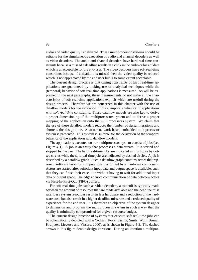
The applications executed on our multiprocessor system consist of jobs (seeFigure 4-1). A job is an entity that processes a data stream. It is started andstopped by the user. The hard real-time jobs are indicated in this figure by dot-ted circles while the soft real-time jobs are indicated by dashed circles. A job isdescribed by a dataflow graph. Such a dataflow graph contains actors that rep-resent software tasks, or computations performed by a hardware component.Actors are started after sufficient input data and output space is available, suchthat they can finish their execution without having to wait for additional inputdata or output space. The edges denote communication of data between actorsvia First-In-First-Out (FIFO) buffers.

For soft real-time jobs such as video decoders, a tradeoff is typically madebetween the amount of resources that are made available and the deadline missrate. Less system resources result in less hardware and a reduction of the hard-ware cost, but also result in a higher deadline miss rate and a reduced quality ofexperience for the end user. It is therefore an objective of the system designerto dimension and program the multiprocessor system in such a way that thequality is minimally compromised for a given resource budget.

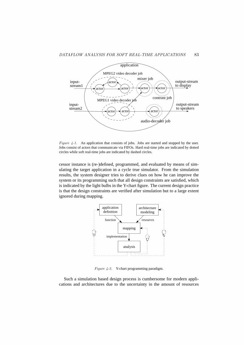
The current design practice of systems that execute soft real-time jobs canbe schematically depicted with a Y-chart (Kock, Essink, Smits, Wolf, Brunel,Kruijtzer, Lieverse and Vissers, 2000), as is shown in Figure 4-2. The dashedarrows in this figure denote design iterations. During an iteration a multipro-

DATAFLOW ANALYSIS FOR SOFT REAL-TIME APPLICATIONS 83

MPEG2 video decoder job

MPEG1 video decoder job

actoractor

actor

actor

actor actor

output-streamto speakers

output-streamto display

input-stream1

stream2input-

application

actor

actor

mixer job

contrast job

audio-decoder job

Figure 4-1. An application that consists of jobs. Jobs are started and stopped by the user.Jobs consist of actors that communicate via FIFOs. Hard real-time jobs are indicated by dottedcircles while soft real-time jobs are indicated by dashed circles.

cessor instance is (re-)defined, programmed, and evaluated by means of sim-ulating the target application in a cycle true simulator. From the simulationresults, the system designer tries to derive clues on how he can improve thesystem or its programming such that all design constraints are satisfied, whichis indicated by the light bulbs in the Y-chart figure. The current design practiceis that the design constraints are verified after simulation but to a large extentignored during mapping.

function resources

implementation

applicationdefinition

architecturemodeling

mapping

analysis

Figure 4-2. Y-chart programming paradigm.

Such a simulation based design process is cumbersome for modern appli-cations and architectures due to the uncertainty in the amount of resources

84 Chapter 4

demanded by the application at run-time and the uncertainty in the amount ofresources supplied by the hardware. The resource demand fluctuates duringexecution because the amount of computation and communication performedby the application often depends on the content of the input stream. For exam-ple, the execution time of the actors depends usually on the values of the inputdata. This can also be the case for the amount of data communicated betweenthe actors. Also, the amount of resources supplied by the hardware fluctuatesdue to arbitration of shared resources in the system. The term “arbitration” isused in this chapter for the local scheduling of actors on processors, as well asfor the policy used to resolve at run-time simultaneous requests for a sharedresource, such as for example a communication bus or a memory port.

Another reason why this simulation based design process has become cum-bersome is that the complexity of system-on-chip designs has grown muchfaster than the increase in speed of the simulators. This has resulted in slowdesign iterations in which usually only a small fraction of the system can beevaluated. It should also be noted that it can be very difficult to find perfor-mance critical corner cases in the design and generate the proper input stimulito observe the system’s behavior for these cases.

Another disadvantage of a simulation based design process is that it canbe difficult to draw conclusions from the simulation results how to adapt themultiprocessor system’s hardware or its programming. It can be difficult todraw conclusions because these multiprocessor systems can exhibit a highlynon-linear behavior.

Finally, we would like to mention that it is difficult to reproduce the sametemporal behavior with such a simulation based design process. The reasonis that the initial state of the arbiters (e.g. Time Division Multiple Access(TDMA) arbiters) in the system is unknown at the moment that the job isstarted. Therefore, the order in which access to a shared resource will begranted by an arbiter is not known at compile time. A different order in whichrequests are granted can result in a completely different temporal behavior of ajob in the case that the same job is started at a different point in time. This willmake it for example impossible to reproduce the same temporal behavior withan (Field Programmable Gate Array (FPGA)) prototype of the system, whichis currently often used to speed up the performance evaluation and debuggingprocess.

In this chapter, we propose a multiprocessor system in which the uncertaintyin the resource supply is bounded by enforcing resource budgets. A resourcebudget is for example a guaranteed amount of time to use a resource such as abus or processor during a predefined period. These enforced resource budgetswill make it possible to share resources, such as a port to background memory,between hard real-time and soft real-time jobs. These budgets also drasticallyreduce the effort to verify the temporal behavior of soft real-time jobs. The

DATAFLOW ANALYSIS FOR SOFT REAL-TIME APPLICATIONS 85

reason is that given enforced resource budgets, the temporal behavior of onejob cannot affect the temporal behavior of another job. This gives a job theillusion that it executes on its own private hardware, so it can be evaluated inisolation.

Given that resource budgets are enforced and guaranteed, then dataflowmodels and their corresponding analysis techniques can be applied to guar-antee that hard real-time jobs will meet their deadlines. However these tech-niques are not directly applicable for soft real-time jobs because they requirethat a schedule can be derived offline. Such a schedule cannot be constructedfor soft real-time jobs because the amount of resources that is provided for softreal-time applications is typicallylessthan the worst-case amount of resourcesthat are needed to meet all deadlines.

In this chapter we advocate the use of a mix of simulation and model basedanalysis techniques for the derivation of the temporal behavior of the soft real-time jobs. We show that dataflow models can be applied by demonstrating thatif resource budgets are enforced that then the effect on the temporal behavior ofrun-time arbitration can be modeled in a dataflow model. These dataflow mod-els can be used for soft real-time jobs to deriveconservativearrival times ofthe data in the system by simulation of this dataflow model. During simulationthe response times of the actors are used instead of the worst-case responsetimes. The response time of an actor depends on the value of the input dataof the actor. The arrival times of the data observed during simulation iscon-servativebecause data will not arrive earlier in the simulator than in the realsystem. There is no need to derive a schedule in advance because the executionorder of actors is determined at run-time by the local schedulers/arbiters. Thesame dataflow models can beanalyzedat compile-time to derive estimates ofthe effects on the throughput and latency of a job when a resource budget isadapted by the designer at compile time. An example of a resource budget isthe capacity of a buffer.

2. RELATED WORKIn this work, dataflow models are used to derive the end-to-end temporal

behavior of jobs. The focus is on synchronous dataflow (SDF) models (Leeand Messerschmitt, 1987), because it is currently the most popular and widelystudied dataflow model for streaming applications with well defined semantics.

A similarity between SDF models and Kahn process networks (Kahn, 1974)is that they can be used to describe streaming applications. However SDFmodels are suitable for static analysis while Kahn process networks are un-suitable. Kahn process networks are unsuitable for static analysis because aKahn process network is Turing complete. Therefore, questions of terminationand bounded buffering are undecidable. That is, no finite time algorithm can

86 Chapter 4

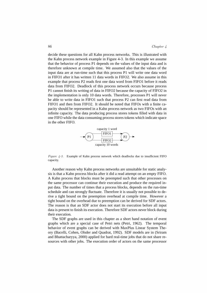
decide these questions for all Kahn process networks. This is illustrated withthe Kahn process network example in Figure 4-3. In this example we assumethat the behavior of process P1 depends on the values of the input data and istherefore unknown at compile time. We assumed also that the values of theinput data are at run-time such that this process P1 will write one data wordin FIFO1 after it has written 11 data words in FIFO2. We also assume in thisexample that process P2 reads first one data word from FIFO1 before it readsdata from FIFO2. Deadlock of this process network occurs because processP1 cannot finish its writing of data in FIFO2 because the capacity of FIFO2 inthe implementation is only 10 data words. Therefore, processes P1 will neverbe able to write data in FIFO1 such that process P2 can first read data fromFIFO1 and then from FIFO2. It should be noted that FIFOs with a finite ca-pacity should be represented in a Kahn process network as two FIFOs with aninfinite capacity. The data producing process stores tokens filled with data inone FIFO while the data consuming process stores tokens which indicate spacein the other FIFO.

FIFO1

capacity 1 word

capacity 10 wordsFIFO2

P1 P2

Figure 4-3. Example of Kahn process network which deadlocks due to insufficient FIFOcapacity.

Another reason why Kahn process networks are unsuitable for static analy-sis is that a Kahn process blocks after it did a read attempt on an empty FIFO.A Kahn process that blocks must be preempted such that other processes onthe same processor can continue their execution and produce the required in-put data. The number of times that a process blocks, depends on the run-timeschedule and can strongly fluctuate. Therefore it is usually not possible to de-rive a tight bound on the preemption overhead at compile time. However atight bound on the overhead due to preemption can be derived for SDF actors.The reason is that an SDF actor does not start its execution before all inputdata is present to finish its execution. Therefore SDF actors never block duringtheir execution.

The SDF graphs are used in this chapter as a short hand notation of eventgraphs which are a special case of Petri nets (Petri, 1962). The temporalbehavior of event graphs can be derived with MaxPlus Linear System The-ory (Bacelli, Cohen, Olsder and Quadrat, 1992). SDF models are in (Sriramand Bhattacharyya, 2000) applied for hard real-time jobs that do not share re-sources with other jobs. The execution order of actors on the same processor

DATAFLOW ANALYSIS FOR SOFT REAL-TIME APPLICATIONS 87

is derived from an offline computed schedule. Similar techniques are appliedin (Poplavko, Basten, Bekooij, Meerbergen and Mesman, 2003) for soft real-time jobs. Good results could only be obtained by taking measures to limit thedifference between the typical and the worst-case response times of the actors.The reason for these good results is that if the difference in response time issmall, then the offline computed execution order is close to the optimal execu-tion order. In this chapter we assume that the processors support preemptionand that the execution order of the actors is determined at run-time. This makesit possible to cope with large variations in the execution time of the actors, andwill allow sharing of resources by actors of different jobs.

In this chapter we advocate the use of a mix of simulation and model basedanalysis techniques for the derivation of the temporal behavior of the soft real-time jobs. The analysis of the temporal behavior of soft real-time jobs is differ-ent from the analysis of hard real-time jobs. The objective of the analysis forhard real-time jobs is to derive the worst-case temporal behavior of the system,while for soft real-time jobs the objective of the analysis is to derive the typ-ical temporal behavior. The typical temporal behavior of jobs depends on thevalues of the input data which are unknown at compile time. Therefore, purelymodel based analysis techniques for hard real-time jobs, such as the techniquesin (Kopetz, 1997; Pop, Eles and Peng, 2002; Richter, Jersak and Ernst, 2003),are not directly applicable for the analysis of soft real-time jobs. The reasonis that the actual values of the input data can be ignored during analysis ofhard real-time jobs because the objective is to derive the worst-case temporalbehavior for any possible input data stream. For soft real-time jobs the valuesof the input data cannot be ignored during analysis because the objective is toderive the typical temporal behavior for a representative input stimuli set. Theuse of probabilistic models, such as Markovian and Poisson models, for thederivation of the typical temporal behavior of soft real-time jobs is either toosimple to characterize the important properties of the source and the system,or too complex for tractable analysis (Zhang, 1995; Sriram and Bhattacharyya,2000). Therefore, simulation is used by us to estimate parameters such as theexecution times of the actors and to test statistical assertions about the tempo-ral behavior of a job that is executed on the system, in a similar way as donein (Hee, 1994).

The concept of reservation based resource allocation has been introducedby the real-time community in order to eliminate interference between thesoftware tasks of soft real-time multimedia jobs that are executed on a singleprocessor system. The enforcement of resource budgets is a service providedby the operating system kernel (Rajkumar, Juwa, Moleno and Oikawa, 1998).The size of the resource budget is determined during a (re)negotiation phasebetween the job and the operating system. In this work, we address multipro-cessor systems in which the resource budgets enforcement is not centralized

88 Chapter 4

but distributed. Resource budgets are reserved to eliminate interference be-tween jobs such that it is possible to share resources between hard real-timeand soft real-time jobs, as well as to obtain a so-called monotonic system (seeSection 4). An important property of a monotonic system is that an increase ofa resource budget of a job cannot result in a reduction of the throughput of thisjob.

3. OUTLINE OF THIS CHAPTERThe organization of this chapter is as follows. The properties of the syn-

chronous dataflow (SDF) model are recapitulated in Section 4. Then in Sec-tion 5 a multiprocessor architecture is presented that is suitable for the deriva-tion of the temporal behavior of jobs with an SDF model. It is shown in Sec-tion 6 that the effects on the temporal behavior of a job, due to TDMA arbi-tration, can be expressed in the SDF model. By simulating this SDF model,conservative and accurate arrival times of tokens can be derived. The sameSDF model is analyzed in Section 7 in order to derive at compile time the sen-sitivity for variations in the execution time of actors on the throughput of thesystem. We show that adaptation of the capacities of the FIFO buffers can re-duce the sensitivity for fluctuations in the execution times of the actors on theend-to-end temporal behavior of a job. To obtain tight bounds on the arrivaltimes of data it may be necessary to make the conditional execution of actorsexplicit in the dataflow model. Section 8 introduces conditional constructs inthe dataflow model that guarantee mutual exclusive execution of actors. Thedataflow graph that is obtained is an analyzable version of a Boolean Data Flow(BDF) graph (Buck, 1993). It is shown that these BDF graphs can be analyzedwith the SDF analysis discussed in Section 4. These conditional constructs areapplied in Section 9 to make explicit that different actors are executed duringI-frame and P-frame decoding in an H263 video decoder. Finally, we state theconclusions in Section 10.

4. DATAFLOW ANALYSISIn this section we define the SDF model and recapitulate its properties. This

SDF model is used in successive sections for the derivation of the temporal be-havior of jobs that are executed on multiprocessor systems with similar char-acteristics as the multiprocessor system that is presented in Section 5.

Before the properties of an SDF model are stated, we first define an SDFgraph as follows:

Definition 1 (Synchronous Data Flow Graph.) The tuple(V,E, d, P, O, I) defines a Synchronous Data Flow (SDF) graph, where

DATAFLOW ANALYSIS FOR SOFT REAL-TIME APPLICATIONS 89

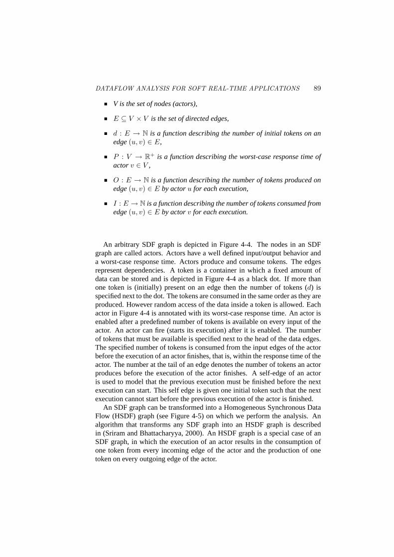
V is the set of nodes (actors),

E ⊆ V × V is the set of directed edges,

d : E → N is a function describing the number of initial tokens on anedge(u, v) ∈ E,

P : V → R+ is a function describing the worst-case response time ofactorv ∈ V ,

O : E → N is a function describing the number of tokens produced onedge(u, v) ∈ E by actoru for each execution,

I : E → N is a function describing the number of tokens consumed fromedge(u, v) ∈ E by actorv for each execution.

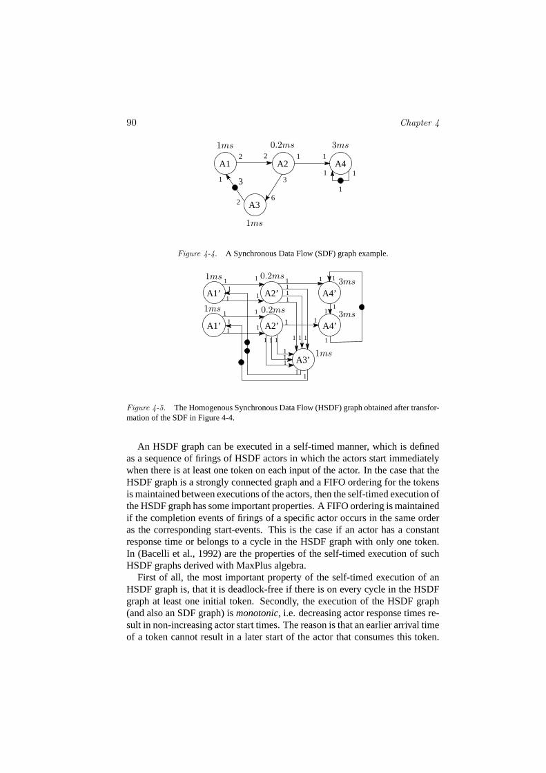
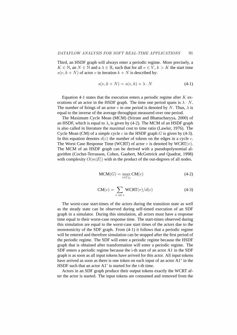
An arbitrary SDF graph is depicted in Figure 4-4. The nodes in an SDFgraph are called actors. Actors have a well defined input/output behavior anda worst-case response time. Actors produce and consume tokens. The edgesrepresent dependencies. A token is a container in which a fixed amount ofdata can be stored and is depicted in Figure 4-4 as a black dot. If more thanone token is (initially) present on an edge then the number of tokens (d) isspecified next to the dot. The tokens are consumed in the same order as they areproduced. However random access of the data inside a token is allowed. Eachactor in Figure 4-4 is annotated with its worst-case response time. An actor isenabled after a predefined number of tokens is available on every input of theactor. An actor can fire (starts its execution) after it is enabled. The numberof tokens that must be available is specified next to the head of the data edges.The specified number of tokens is consumed from the input edges of the actorbefore the execution of an actor finishes, that is, within the response time of theactor. The number at the tail of an edge denotes the number of tokens an actorproduces before the execution of the actor finishes. A self-edge of an actoris used to model that the previous execution must be finished before the nextexecution can start. This self edge is given one initial token such that the nextexecution cannot start before the previous execution of the actor is finished.

An SDF graph can be transformed into a Homogeneous Synchronous DataFlow (HSDF) graph (see Figure 4-5) on which we perform the analysis. Analgorithm that transforms any SDF graph into an HSDF graph is describedin (Sriram and Bhattacharyya, 2000). An HSDF graph is a special case of anSDF graph, in which the execution of an actor results in the consumption ofone token from every incoming edge of the actor and the production of onetoken on every outgoing edge of the actor.

90 Chapter 4

A2 A4A1

6A3

1ms

1ms 0.2ms 3ms2 2 1 1

3

2

311

11

Figure 4-4. A Synchronous Data Flow (SDF) graph example.

A4’

A4’

1

11

A2’A1’

A2’A1’

1

1

11

1

111

11

1

1

11

1

1

1

1

1

1

1

1 1

1

1

A3’1ms

0.2ms1ms

1ms 0.2ms1

1

1

1

3ms

3ms

Figure 4-5. The Homogenous Synchronous Data Flow (HSDF) graph obtained after transfor-mation of the SDF in Figure 4-4.

An HSDF graph can be executed in a self-timed manner, which is definedas a sequence of firings of HSDF actors in which the actors start immediatelywhen there is at least one token on each input of the actor. In the case that theHSDF graph is a strongly connected graph and a FIFO ordering for the tokensis maintained between executions of the actors, then the self-timed execution ofthe HSDF graph has some important properties. A FIFO ordering is maintainedif the completion events of firings of a specific actor occurs in the same orderas the corresponding start-events. This is the case if an actor has a constantresponse time or belongs to a cycle in the HSDF graph with only one token.In (Bacelli et al., 1992) are the properties of the self-timed execution of suchHSDF graphs derived with MaxPlus algebra.

First of all, the most important property of the self-timed execution of anHSDF graph is, that it is deadlock-free if there is on every cycle in the HSDFgraph at least one initial token. Secondly, the execution of the HSDF graph(and also an SDF graph) ismonotonic, i.e. decreasing actor response times re-sult in non-increasing actor start times. The reason is that an earlier arrival timeof a token cannot result in a later start of the actor that consumes this token.

DATAFLOW ANALYSIS FOR SOFT REAL-TIME APPLICATIONS 91

Third, an HSDF graph will always enter a periodic regime. More precisely, aK ∈ N, anN ∈ N and aλ ∈ R, such that for allv ∈ V , k > K the start times(v, k + N) of actorv in iterationk + N is described by:

s(v, k + N) = s(v, k) + λ ·N (4-1)

Equation 4-1 states that the execution enters a periodic regime afterK ex-ecutions of an actor in the HSDF graph. The time one period spans isλ · N .The number of firings of an actorv in one period is denoted byN . Thus,λ isequal to the inverse of the average throughput measured over one period.

The Maximum Cycle Mean (MCM) (Sriram and Bhattacharyya, 2000) ofan HSDF, which is equal toλ, is given by (4-2). The MCM of an HSDF graphis also called in literature the maximal cost to time ratio (Lawler, 1976). TheCycle Mean (CM) of a simple cyclec in the HSDF graphG is given by (4-3).In this equation denotesd(c) the number of tokens on the edges in a cyclec.The Worst Case Response Time (WCRT) of actorv is denoted by WCRT(v).The MCM of an HSDF graph can be derived with a pseudopolynomial al-gorithm (Cochet-Terrasson, Cohen, Gaubert, McGettrick and Quadrat, 1998)with complexityO(m|E|) with m the product of the out-degrees of all nodes.

MCM(G) = maxc∈CG

CM(c) (4-2)

CM(c) =∑

v on c

WCRT(v)/d(c) (4-3)

The worst-case start-times of the actors during the transition state as wellas the steady state can be observed during self-timed execution of an SDFgraph in a simulator. During this simulation, all actors must have a responsetime equal to their worst-case response time. The start-times observed duringthis simulation are equal to the worst-case start times of the actors due to themonotonicity of the SDF graph. From (4-1) it follows that a periodic regimewill be entered and therefore simulation can be stopped after the first period ofthe periodic regime. The SDF will enter a periodic regime because the HSDFgraph that is obtained after transformation will enter a periodic regime. TheSDF enters a periodic regime because the i-th start of an actor A1 in the SDFgraph is as soon as all input tokens have arrived for this actor. All input tokenshave arrived as soon as there is one token on each input of an actor A1’ in theHSDF such that an actor A1’ is started for the i-th time.

Actors in an SDF graph produce their output tokens exactly the WCRT af-ter the actor is started. The input tokens are consumed and removed from the

92 Chapter 4

input exactly the WCRT after the actor is started. Code segments in the imple-mentation can be represented by an SDF actor in the model. Code segmentsproduce the output tokens and consume the input tokens within the WCRT ofthe actor. The arrival times of tokens during selftimed execution of the SDFgraph is not earlier then in the implementation due to the monotonic behaviorof a selftimed executed SDF graph. Therefore an upper bound on the arrivaltime of tokens is observed during selftimed execution of the SDF graph.

We refer in this chapter to a code segment as an actor in the implementation.The actors in the implementation have a response time as well as an ExecutionTime (ET). The ET of an actor in the implementation is defined as the intervalof time it takes to execute the corresponding code segment on a processorwithout that its execution is preempted. The execution time depends often onthe values of the input data. The Worst Case Execution Time (WCET) is anupper bound on the execution time of an actor in the implementation and isderived with static program analysis techniques (Li and Malik, 1999).

It should be noted that the token arrival times during selftimed executionin the SDF simulator remain conservative if the Response Times (RTs) of theactors are used instead of the worst-case response times of the actors. TheRT of an actor is an upperbound on the time interval between the point intime that the actor is enabled and that the point in time that the actor finishesits execution. The response time of an actor can depend on the values of theinput data that are consumed during that execution. The token arrival timesduring selftimed execution in the SDF simulator are conservative because theselftimed execution of the SDF graph is monotonic. The use of the RTs ofactors allows use to derive an upperbound on the token arrival times for softreal-time jobs given a specific input stimuli set for that job.

In Section 7 we will use Predicted Response Times (PRTs) of the actors toderive at compile time the resource budgets of soft real-time jobs. The PRTof an actor is the measured average response time of this actor on a processorgiven a specific input stimuli set for that actor. Given the PRT of an actor wewill predict the resource budget for a soft real-time job.

5. MULTIPROCESSOR SYSTEM TEMPLATEThis section describes a network based multiprocessor system. This multi-

processor system is defined in such a way that a tight bound on the temporalbehavior of jobs can be derived at compile time with dataflow analysis tech-niques. These analysis techniques are described in the previous section and areextended in Section 6.

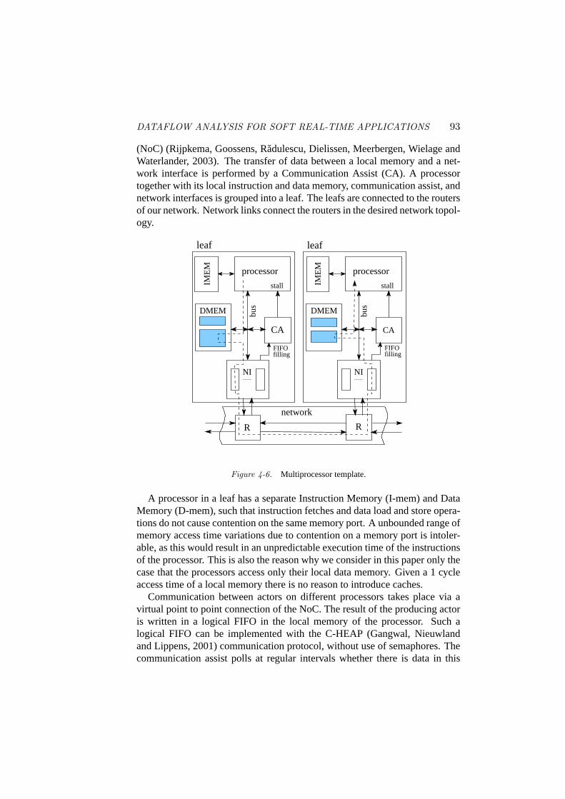
Figure 4-6 shows the architecture template of this multiprocessor system.The processors in this template are, together with their local data memory,connected to the Network Interface (NI) of a packet switched Network on Chip

DATAFLOW ANALYSIS FOR SOFT REAL-TIME APPLICATIONS 93

(NoC) (Rijpkema, Goossens, Radulescu, Dielissen, Meerbergen, Wielage andWaterlander, 2003). The transfer of data between a local memory and a net-work interface is performed by a Communication Assist (CA). A processortogether with its local instruction and data memory, communication assist, andnetwork interfaces is grouped into a leaf. The leafs are connected to the routersof our network. Network links connect the routers in the desired network topol-ogy.

FIFOfilling

FIFOfilling

leaf leaf

IME

M

IME

M

bus

bus

RR

stallstall

CA CA

DMEM

NINI

DMEM

network

processor processor

Figure 4-6. Multiprocessor template.

A processor in a leaf has a separate Instruction Memory (I-mem) and DataMemory (D-mem), such that instruction fetches and data load and store opera-tions do not cause contention on the same memory port. A unbounded range ofmemory access time variations due to contention on a memory port is intoler-able, as this would result in an unpredictable execution time of the instructionsof the processor. This is also the reason why we consider in this paper only thecase that the processors access only their local data memory. Given a 1 cycleaccess time of a local memory there is no reason to introduce caches.

Communication between actors on different processors takes place via avirtual point to point connection of the NoC. The result of the producing actoris written in a logical FIFO in the local memory of the processor. Such alogical FIFO can be implemented with the C-HEAP (Gangwal, Nieuwlandand Lippens, 2001) communication protocol, without use of semaphores. Thecommunication assist polls at regular intervals whether there is data in this

94 Chapter 4

FIFO. As soon as the CA detects that there is data available, it copies thedata into a FIFO of the NI. There is one private FIFO per connection in the NI.Subsequently the data is transported over the network to the NI of the receivingprocessor. As soon as the data arrives in this NI, it is copied by the CA intoa logical FIFO in the memory of the processor that executes the consumingactor. The data is read from this FIFO after the consuming actor has detectedthat there is sufficient data in the FIFO. Flow control between the producingand consuming actor is achieved by making sure that data is not written into aFIFO before it is checked that there is space available in this FIFO.

Data is stored in the local memory of the processor before it is transferredacross the network. This done for a number of reasons. First of all, the band-width of a connection is set by configuring tables in the network for a longerperiod of time. The bandwidth reserved for a connection will typically be lessthan the peak data rate generated by the producing actor. Therefore a bufferis needed between the processor and the network to average out the peak datarate such that the bandwidth provided by the network is well utilized. Alsothe memory in the leaf which receives the data can typically not accommodatethe peak bandwidth because another processor can access this memory at thesame time. Another reason is that without such a buffer the execution timeand the response time of the actors is dependent on the allocated bandwidthin the network. This dependency will complicate the analysis of the temporalbehavior.

The size of the buffer in which data is stored before it is transferred acrossthe network is significant, given the assumption that the actors produce largechunks of data at large intervals. On the other hand, the network will transfervery small chunks of data (3 words of 32 bits) at very small intervals (∼2 ns).Given that large memories are inherently slow, it is desirable to split the largelogical FIFO between the processor and the network, in a small (∼32 word)dedicated FIFO per connection in the network interface, and a large logicalFIFO in the local memory of the processor. The task of the CA is to copy thedata between FIFOs in the NI and FIFOs in local memory of the processor.

The CA is also responsible for the arbitration of the data memory bus. Theapplied arbitration scheme is such that a low worst-case latency of memorystore and load operations is obtained and that a minimal throughput and max-imal latency per connection is guaranteed. A more detailed description can befound in (Bekooij, Moreira, Poplavko, Mesman, Pastrnak and van Meerbergen,2004).

In the proposed architecture, the communication between actors that runon different processors has a guaranteed minimal throughput and a maximallatency. Given these characteristics, the communication can be modeled as if ittakes place through completely independent virtual point-to-point connections.These connections can be modeled together with the actors of a job in one SDF

DATAFLOW ANALYSIS FOR SOFT REAL-TIME APPLICATIONS 95

graph (Poplavko et al., 2003). Given this SDF graph, the guaranteed minimalthroughput of a hard real-time job can be determined.

6. RESOURCE ARBITRATIONIn this section, we show that the resource conflicts that are resolved at run-

time by TDMA arbiters, can be taken into account in an SDF model. Conser-vative token arrival times are observed during self-timed execution of this SDFmodel in a simulator. The same SDF model is analyzed in Section 7 to obtainthe sensitivity for fluctuations in the response times of actors on the temporalbehavior of a job.

Resource conflicts can occur if multiple actors execute on one processor.These resource conflicts can be resolved at compile time or at run time. Theresource conflicts can be resolved at compile time by computing offline a validschedule for the SDF graph under consideration. In the static order schedulingapproach (Sriram and Bhattacharyya, 2000), the execution order of the actorsin this offline computed schedule is enforced at run time. If the static orderscheduling approach is applied, then a decrease in response time of actors canonly result in an earlier arrival of tokens and an increase in throughput of thesystem. The reason is that there is a one to one correspondence between actorsin the system and the actors in the SDF model and that it is known that theself-timed execution of the SDF model is monotonic (see Section 4).

An important disadvantage of the static order scheduling approach is thatit cannot be applied if the execution of actors is conditional, as is the casein the H263 video decoder example in Section 9. The execution of actors isconditional if a value of a token determines whether an actor will be executedor not. In a static order schedule it can occur that if, for example, actor A isnot executed, then another actor B will wait forever for a token produced byactor A. Other actors on the same processor as actor B will not be executed aslong as actor B waits for the token because the execution order of actors on thesame processor is predefined and fixed.

Resource conflicts can also be resolved at run time by an arbiter (localscheduler). In the case that arbitration is performed at run time, the arrivalof tokens determines whether an actor will be executed or not, and what theexecution order of the actors on a processor will be. In the case that, for ex-ample, TDMA arbitration is applied, then the effects of the TDMA arbitrationon the arrival time of the tokens can be taken into account in the responsetimes of the actors in the SDF model. A proof that TDMA arbitration can bemodeled implicitly in the response time of an actor is presented in the nextparagraphs. This proof demonstrates with mathematical induction that tokenswill not arrive later in the implementation than during selftimed execution of anHSDF model. It is sufficient to prove for one actor executed during a TDMA

96 Chapter 4

time slice on a processor that the actor will not produce tokens later in the im-plementation than in the HSDF model because the selftimed execution of anHSDF model is monotonic.

In this proof, an abstract representation of a processor is used which exe-cutes actor A1 during intervalT1 in a periodT . This representation is shownin Figure 4-9. Actor A1 starts its execution during intervalT1, as soon as theprevious execution of actor A1 has finished and an input token has arrived.If actor A1 did not finish its execution at the end of the intervalT1 then thisactor will be preempted and it will continue its execution in the next period.The additional time due to context switches can be included in the (worst-case)response time of an actor, because the maximum number of context switchesthat can happen during the execution of an actor is known at compile time. Thetime p(j) denotes the execution time of the j-th execution of actor A1 when itexecutes on the processor without being preempted.

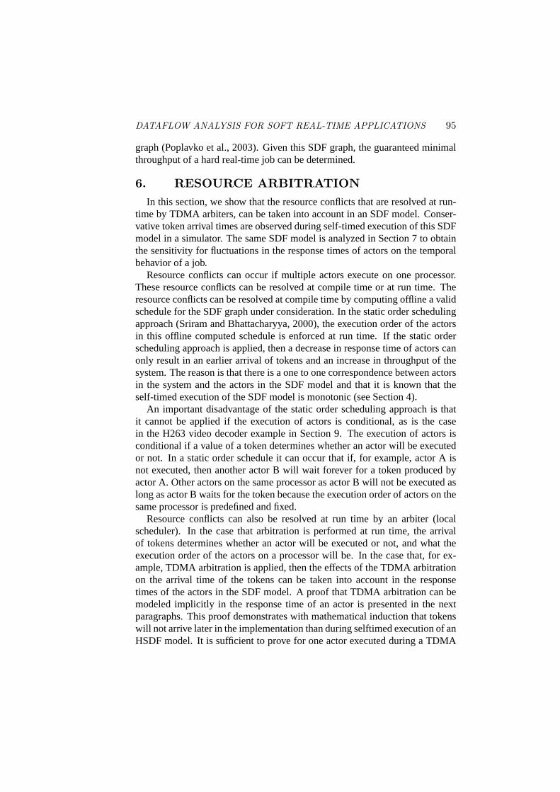
Two cases should be distinguished to determine the response time of anactor. An actor can start at the begin of the intervalT1 or during the intervalT1. If the actor starts at the begin of an interval andp(j) = 2.5 T1 then thisactor will be preempted twice, as is shown in Figure 4-7. Given that the actoris preempted twice then the actor will finish its executionp(j) + 2(T − T1)after it is started. In other words the Interruption time (I1) of the actor is in thiscase according to (4-4).

t(s)T1

T

Figure 4-7. Stretch of the response time of an actor due to preemption in the case that theactor starts at the begin of intervalT1.

I1(j) = (T − T1)(⌈

p(j)T1

⌉− 1) (4-4)

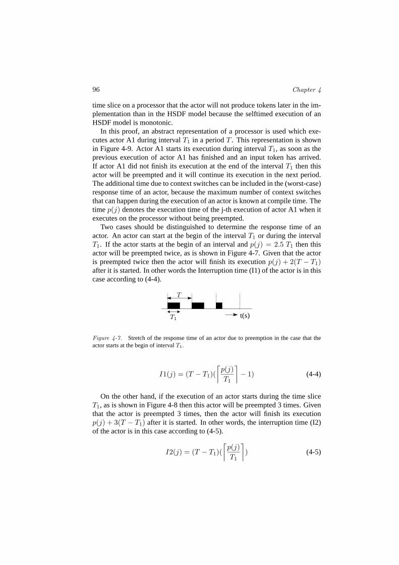
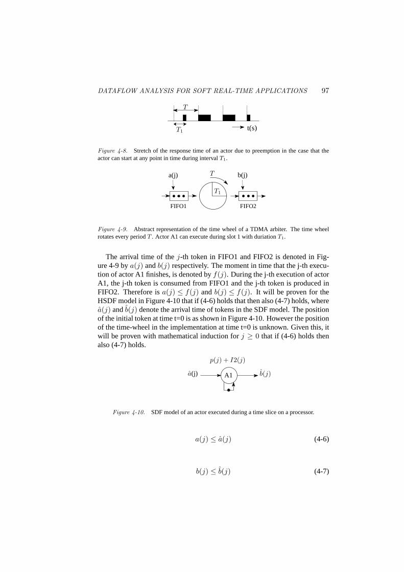
On the other hand, if the execution of an actor starts during the time sliceT1, as is shown in Figure 4-8 then this actor will be preempted 3 times. Giventhat the actor is preempted 3 times, then the actor will finish its executionp(j) + 3(T − T1) after it is started. In other words, the interruption time (I2)of the actor is in this case according to (4-5).

I2(j) = (T − T1)(⌈

p(j)T1

⌉) (4-5)

DATAFLOW ANALYSIS FOR SOFT REAL-TIME APPLICATIONS 97

t(s)T1

T

Figure 4-8. Stretch of the response time of an actor due to preemption in the case that theactor can start at any point in time during intervalT1.

FIFO2FIFO1

a(j) b(j)

T1

T

Figure 4-9. Abstract representation of the time wheel of a TDMA arbiter. The time wheelrotates every periodT . Actor A1 can execute during slot 1 with duriationT1.

The arrival time of thej-th token in FIFO1 and FIFO2 is denoted in Fig-ure 4-9 bya(j) andb(j) respectively. The moment in time that the j-th execu-tion of actor A1 finishes, is denoted byf(j). During the j-th execution of actorA1, the j-th token is consumed from FIFO1 and the j-th token is produced inFIFO2. Therefore isa(j) ≤ f(j) andb(j) ≤ f(j). It will be proven for theHSDF model in Figure 4-10 that if (4-6) holds that then also (4-7) holds, wherea(j) andb(j) denote the arrival time of tokens in the SDF model. The positionof the initial token at time t=0 is as shown in Figure 4-10. However the positionof the time-wheel in the implementation at time t=0 is unknown. Given this, itwill be proven with mathematical induction forj ≥ 0 that if (4-6) holds thenalso (4-7) holds.

A1a(j) b(j)

p(j) + I2(j)

Figure 4-10. SDF model of an actor executed during a time slice on a processor.

a(j) ≤ a(j) (4-6)

b(j) ≤ b(j) (4-7)

98 Chapter 4

Given that the position of the time-wheel of the implementation is unknownand that initially actor A1 does not execute thenf(0) is:

f(0) ≤ a(0) + p(0) + max(I1(0), I2(0)) ≤ a(0) + p(0) + I2(0) (4-8)

For the arrival time of the first output token in the HSDF model it holds that:

b(0) = a(0) + p(0) + I2 (4-9)

From (4-6), (4-9) and (4-8) it follows that:

f(0) ≤ b(0) (4-10)

Now we want to establish our inductive step by showing how the truth ofour induction hypothesis in (4-11) forces us to accept thatf(j +1) ≤ b(j +1).

f(j) ≤ b(j) (4-11)

For the implementation andj ≥ 0 the following equations hold in whichthe intermediate variablestx andty are defined:

tx = a(j + 1) + p(j + 1) + max(T − T1 + I1(j + 1), I2(j + 1)) (4-12)

ty = f(j) + p(j + 1) + max(T − T1 + I1(j + 1), I2(j + 1)) (4-13)

f(j + 1) ≤ max(tx, ty) (4-14)

Equation 4-14 can be rewritten as:

f(j + 1) ≤ max(f(j), a(j + 1)) + p(j + 1) + I2(j + 1) (4-15)

Equation 4-14 holds because: ifa(j+1) > f(j) then tokenj+1 has arrivedafter the j-th execution of actor A1 has finished (see Figure 4-11). After arrival

DATAFLOW ANALYSIS FOR SOFT REAL-TIME APPLICATIONS 99

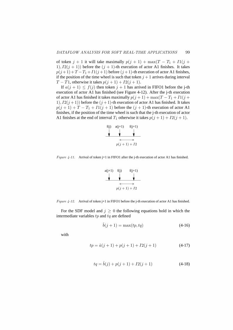
of token j + 1 it will take maximally p(j + 1) + max(T − T1 + I1(j +1), I2(j + 1)) before the(j + 1)-th execution of actor A1 finishes. It takesp(j +1)+T −T1 + I1(j +1) before(j +1)-th execution of actor A1 finishes,if the position of the time wheel is such that tokenj + 1 arrives during intervalT − T1, otherwise it takesp(j + 1) + I2(j + 1).

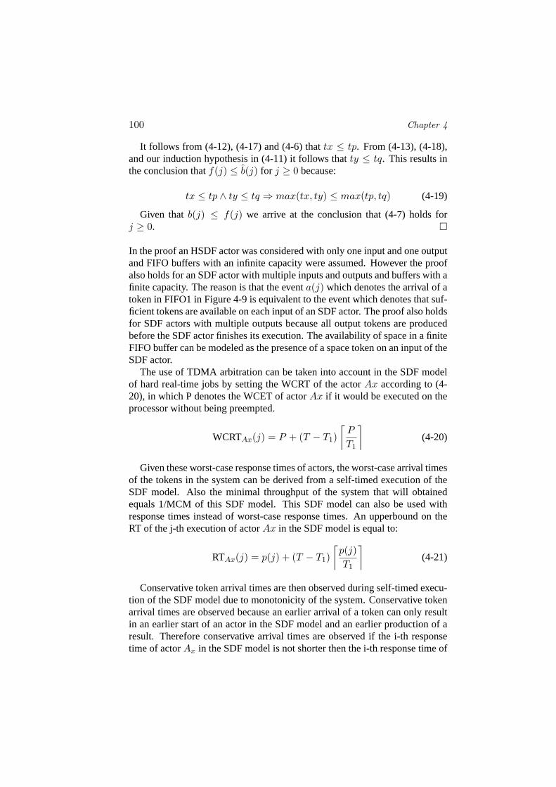
If a(j + 1) ≤ f(j) then tokenj + 1 has arrived in FIFO1 before the j-thexecution of actor A1 has finished (see Figure 4-12). After the j-th executionof actor A1 has finished it takes maximallyp(j + 1) + max(T − T1 + I1(j +1), I2(j +1)) before the(j +1)-th execution of actor A1 has finished. It takesp(j + 1) + T − T1 + I1(j + 1) before the(j + 1)-th execution of actor A1finishes, if the position of the time wheel is such that the j-th execution of actorA1 finishes at the end of intervalT1 otherwise it takesp(j + 1) + I2(j + 1).

f(j)

p(j + 1) + I2

f(j+1)a(j+1)

Figure 4-11. Arrival of token j+1 in FIFO1 after the j-th execution of actor A1 has finished.

a(j+1)

p(j + 1) + I2

f(j+1)f(j)

Figure 4-12. Arrival of token j+1 in FIFO1 before the j-th execution of actor A1 has finished.

For the SDF model andj ≥ 0 the following equations hold in which theintermediate variablestp andtq are defined

b(j + 1) = max(tp, tq) (4-16)

with

tp = a(j + 1) + p(j + 1) + I2(j + 1) (4-17)

tq = b(j) + p(j + 1) + I2(j + 1) (4-18)

100 Chapter 4

It follows from (4-12), (4-17) and (4-6) thattx ≤ tp. From (4-13), (4-18),and our induction hypothesis in (4-11) it follows thatty ≤ tq. This results inthe conclusion thatf(j) ≤ b(j) for j ≥ 0 because:

tx ≤ tp ∧ ty ≤ tq ⇒ max(tx, ty) ≤ max(tp, tq) (4-19)

Given thatb(j) ≤ f(j) we arrive at the conclusion that (4-7) holds forj ≥ 0. �

In the proof an HSDF actor was considered with only one input and one outputand FIFO buffers with an infinite capacity were assumed. However the proofalso holds for an SDF actor with multiple inputs and outputs and buffers with afinite capacity. The reason is that the eventa(j) which denotes the arrival of atoken in FIFO1 in Figure 4-9 is equivalent to the event which denotes that suf-ficient tokens are available on each input of an SDF actor. The proof also holdsfor SDF actors with multiple outputs because all output tokens are producedbefore the SDF actor finishes its execution. The availability of space in a finiteFIFO buffer can be modeled as the presence of a space token on an input of theSDF actor.

The use of TDMA arbitration can be taken into account in the SDF modelof hard real-time jobs by setting the WCRT of the actorAx according to (4-20), in which P denotes the WCET of actorAx if it would be executed on theprocessor without being preempted.

WCRTAx(j) = P + (T − T1)⌈

P

T1

⌉(4-20)

Given these worst-case response times of actors, the worst-case arrival timesof the tokens in the system can be derived from a self-timed execution of theSDF model. Also the minimal throughput of the system that will obtainedequals 1/MCM of this SDF model. This SDF model can also be used withresponse times instead of worst-case response times. An upperbound on theRT of the j-th execution of actorAx in the SDF model is equal to:

RTAx(j) = p(j) + (T − T1)⌈

p(j)T1

⌉(4-21)

Conservative token arrival times are then observed during self-timed execu-tion of the SDF model due to monotonicity of the system. Conservative tokenarrival times are observed because an earlier arrival of a token can only resultin an earlier start of an actor in the SDF model and an earlier production of aresult. Therefore conservative arrival times are observed if the i-th responsetime of actorAx in the SDF model is not shorter then the i-th response time of

DATAFLOW ANALYSIS FOR SOFT REAL-TIME APPLICATIONS 101

actorAx in the implementation. This is the case if response times accordingto ( 4-21) are used in the SDF model. An important advantage of the use ofan SDF model instead of cycle true simulation model of the system is that thearrival time of tokens during self-timed execution is conservative while thisis not the case for a cycle true simulation model. The reason is that the initialposition of the time wheels in the system at time t=0 is not known. Another ad-vantage is that execution of the SDF model will be much faster than simulationof a cycle true model because an SDF model is a more abstract model.

7. SENSITIVITY ANALYSIS & REDUCTIONThis section describes dataflow analysis techniques that are used to deter-

mine the FIFOs of which the capacity should be increased, in order to reducethe sensitivity of a soft real-time job, for fluctuations in the response times ofthe actors. A lower sensitivity of a job will reduce the deadline miss rate whichenhances the quality of experience of the user.

For soft real-time jobs a predicted MCM can be calculated with (4-2) giventhe resource budgets of a job and by using the predicted response times of theactors instead of the WCRT of the actors. Here it is assumed that the PRT ofan actor is equal to the average response time of this actor on a processor withTDMA arbitration and representative input data.

It is obvious that this predicted MCM is not smaller than the actual MCMif the response times of the actors is smaller than the PRT of the actors. Thepredicted MCM is also not smaller than the actual MCM if the cycle mean ofa cycle in the SDF graph, to which the actors belong that have an RT largerthan their PRT, does not exceed the predicted MCM. The Cycle Mean (CM) isdefined in (4-3). In other words the temporal behavior of a job is more sensitivefor deviations in the response times of actors which belong to cycles of whichthe CM is likely to be larger than the predicted MCM. By increasing the FIFOscapacity, the CM of these cycles can be decreased such that the job becomesless sensitive.

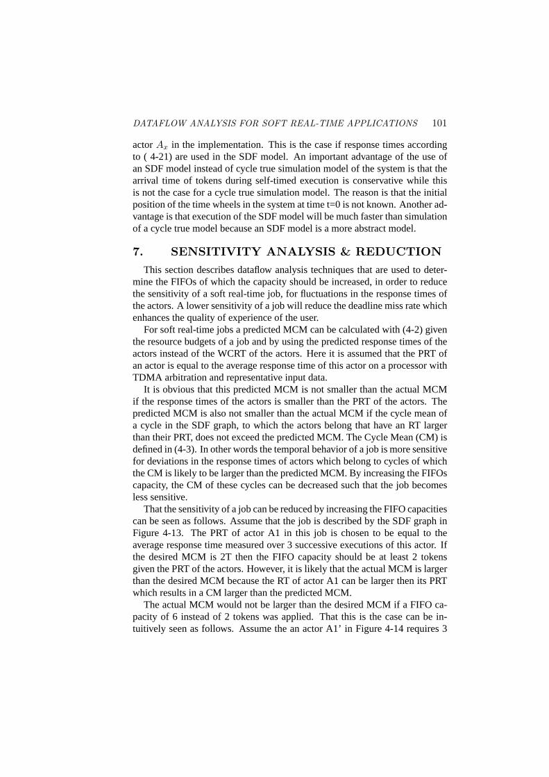
That the sensitivity of a job can be reduced by increasing the FIFO capacitiescan be seen as follows. Assume that the job is described by the SDF graph inFigure 4-13. The PRT of actor A1 in this job is chosen to be equal to theaverage response time measured over 3 successive executions of this actor. Ifthe desired MCM is 2T then the FIFO capacity should be at least 2 tokensgiven the PRT of the actors. However, it is likely that the actual MCM is largerthan the desired MCM because the RT of actor A1 can be larger then its PRTwhich results in a CM larger than the predicted MCM.

The actual MCM would not be larger than the desired MCM if a FIFO ca-pacity of 6 instead of 2 tokens was applied. That this is the case can be in-tuitively seen as follows. Assume the an actor A1’ in Figure 4-14 requires 3

102 Chapter 4

2

A0 A11

11 1

11

1

1PRT=2T PRT=2T

Figure 4-13. SDF with a predicted MCM of 2T.

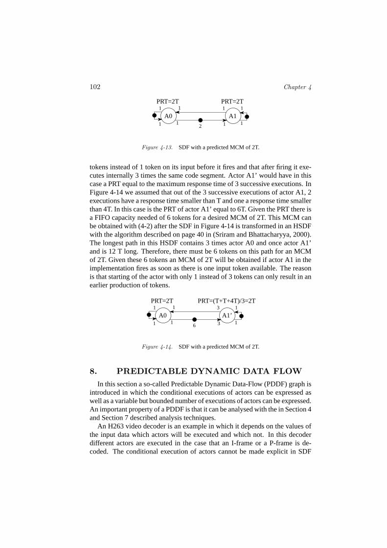
tokens instead of 1 token on its input before it fires and that after firing it exe-cutes internally 3 times the same code segment. Actor A1’ would have in thiscase a PRT equal to the maximum response time of 3 successive executions. InFigure 4-14 we assumed that out of the 3 successive executions of actor A1, 2executions have a response time smaller than T and one a response time smallerthan 4T. In this case is the PRT of actor A1’ equal to 6T. Given the PRT there isa FIFO capacity needed of 6 tokens for a desired MCM of 2T. This MCM canbe obtained with (4-2) after the SDF in Figure 4-14 is transformed in an HSDFwith the algorithm described on page 40 in (Sriram and Bhattacharyya, 2000).The longest path in this HSDF contains 3 times actor A0 and once actor A1’and is 12 T long. Therefore, there must be 6 tokens on this path for an MCMof 2T. Given these 6 tokens an MCM of 2T will be obtained if actor A1 in theimplementation fires as soon as there is one input token available. The reasonis that starting of the actor with only 1 instead of 3 tokens can only result in anearlier production of tokens.

PRT=2T PRT=(T+T+4T)/3=2T

6

A0 A1’1

11 3

11

1

3

Figure 4-14. SDF with a predicted MCM of 2T.

8. PREDICTABLE DYNAMIC DATA FLOWIn this section a so-called Predictable Dynamic Data-Flow (PDDF) graph is

introduced in which the conditional executions of actors can be expressed aswell as a variable but bounded number of executions of actors can be expressed.An important property of a PDDF is that it can be analysed with the in Section 4and Section 7 described analysis techniques.

An H263 video decoder is an example in which it depends on the values ofthe input data which actors will be executed and which not. In this decoderdifferent actors are executed in the case that an I-frame or a P-frame is de-coded. The conditional execution of actors cannot be made explicit in SDF

DATAFLOW ANALYSIS FOR SOFT REAL-TIME APPLICATIONS 103

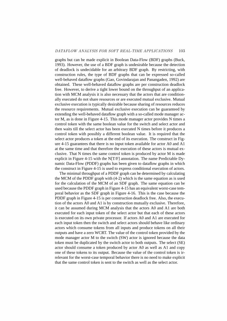
graphs but can be made explicit in Boolean Data-Flow (BDF) graphs (Buck,1993). However, the use of a BDF graph is undesirable because the detectionof deadlock is undecidable for an arbitrary BDF graph. By restricting, withconstruction rules, the type of BDF graphs that can be expressed so-calledwell-behaved dataflow graphs (Gao, Govindarajan and Panangaden, 1992) areobtained. These well-behaved dataflow graphs are per construction deadlockfree. However, to derive a tight lower bound on the throughput of an applica-tion with MCM analysis it is also necessary that the actors that are condition-ally executed do not share resources or are executed mutual exclusive. Mutualexclusive execution is typically desirable because sharing of resources reducesthe resource requirements. Mutual exclusive execution can be guaranteed byextending the well-behaved dataflow graph with a so-called mode manager ac-tor M, as is done in Figure 4-15. This mode manager actor provides N times acontrol token with the same boolean value for the switch and select actor andthen waits till the select actor has been executed N times before it produces acontrol token with possibly a different boolean value. It is required that theselect actor produces a token at the end of its execution. The construct in Fig-ure 4-15 guarantees that there is no input token available for actor A0 and A1at the same time and that therefore the execution of these actors is mutual ex-clusive. That N times the same control token is produced by actor M is madeexplicit in Figure 4-15 with the N[T/F] annotation. The name Predictable Dy-namic Data-Flow (PDDF) graphs has been given to dataflow graphs in whichthe construct in Figure 4-15 is used to express conditional execution of actors.

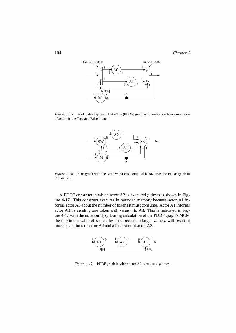
The minimal throughput of a PDDF graph can be determined by calculatingthe MCM of the PDDF graph with (4-2) which is the same equation as is usedfor the calculation of the MCM of an SDF graph. The same equation can beused because the PDDF graph in Figure 4-15 has an equivalent worst-case tem-poral behavior as the SDF graph in Figure 4-16. This is the case because thePDDF graph in Figure 4-15 is per construction deadlock free. Also, the execu-tion of the actors A0 and A1 is by construction mutually exclusive. Therefore,it can be assumed during MCM analysis that the actors A0 and A1 are bothexecuted for each input token of the select actor but that each of these actorsis executed on its own private processor. If actors A0 and A1 are executed foreach input token then the switch and select actors should behave like ordinaryactors which consume tokens from all inputs and produce tokens on all theiroutputs and have a zero WCRT. The value of the control token provided by themode manager actor M to the switch (SW) actor is ignored because the datatoken must be duplicated by the switch actor to both outputs. The select (SE)actor should consume a token produced by actor A0 as well as A1 and copyone of these tokens to its output. Because the value of the control token is ir-relevant for the worst-case temporal behavior there is no need to make explicitthat the same control token is sent to the switch as well as the select actor.

104 Chapter 4

N

T

F

T

F

M1

N[T/F]

1 111

11

1

1 1A1

1

N

select-actorswitch-actor

A0

1 1

Figure 4-15. Predictable Dynamic DataFlow (PDDF) graph with mutual exclusive executionof actors in the True and False branch.

N

1SE

1

1SW

1

11

1A0

A11 1

1 1

M

N NN1

1 1

Figure 4-16. SDF graph with the same worst-case temporal behavior as the PDDF graph inFigure 4-15.

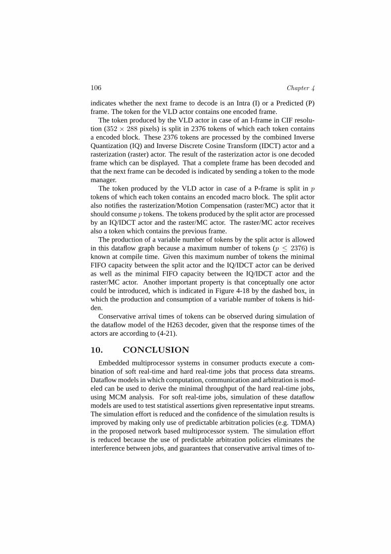
A PDDF construct in which actor A2 is executedp times is shown in Fig-ure 4-17. This construct executes in bounded memory because actor A1 in-forms actor A3 about the number of tokens it must consume. Actor A1 informsactor A3 by sending one token with valuep to A3. This is indicated in Fig-ure 4-17 with the notation 1[p]. During calculation of the PDDF graph’s MCMthe maximum value ofp must be used because a larger valuep will result inmore executions of actor A2 and a later start of actor A3.

1 1 p1 p 1A1 A2 A3

1[n]1[p]

Figure 4-17. PDDF graph in which actor A2 is executedp times.

DATAFLOW ANALYSIS FOR SOFT REAL-TIME APPLICATIONS 105

9. DATAFLOW MODEL OF AN H263 VIDEODECODER

A dataflow model of an H263 video decoder is presented in this sectionwhich illustrates the use of the modeling techniques that were introduced in theprevious sections. This H263 video decoder is a soft real-time job of which thevalues of the input data determine whether some of the actors will be executedor not. Also the number of tokens produced and consumed by the actors can bedata dependent. Despite the dynamic behavior of this job, it remains possibleto derive the minimal capacity of the FIFOs as well as conservative arrivaltimes of tokens with a dataflow model.

11

1

sink

MCraster/

1

1 1

demux

1

1

1(T/F)

bitstreamencoded

mode

VLD

split split

1 12376

11 1

1

123761

IDCTIQ/ IQ/

IDCT

111

to display

111 1

1

1

FT T F

T F

1

p

11

1

1

1 11

1

1

1

1

11

1

1

1

1

1

1

1

1

raster

1[p]

1[p]

1

p

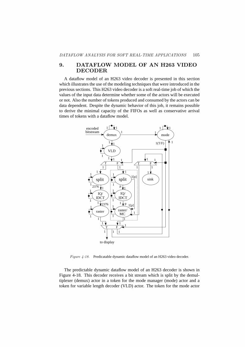
Figure 4-18. Predicatable dynamic dataflow model of an H263 video decoder.

The predictable dynamic dataflow model of an H263 decoder is shown inFigure 4-18. This decoder receives a bit stream which is split by the demul-tiplexer (demux) actor in a token for the mode manager (mode) actor and atoken for variable length decoder (VLD) actor. The token for the mode actor

106 Chapter 4

indicates whether the next frame to decode is an Intra (I) or a Predicted (P)frame. The token for the VLD actor contains one encoded frame.

The token produced by the VLD actor in case of an I-frame in CIF resolu-tion (352 × 288 pixels) is split in 2376 tokens of which each token containsa encoded block. These 2376 tokens are processed by the combined InverseQuantization (IQ) and Inverse Discrete Cosine Transform (IDCT) actor and arasterization (raster) actor. The result of the rasterization actor is one decodedframe which can be displayed. That a complete frame has been decoded andthat the next frame can be decoded is indicated by sending a token to the modemanager.

The token produced by the VLD actor in case of a P-frame is split inptokens of which each token contains an encoded macro block. The split actoralso notifies the rasterization/Motion Compensation (raster/MC) actor that itshould consumep tokens. The tokens produced by the split actor are processedby an IQ/IDCT actor and the raster/MC actor. The raster/MC actor receivesalso a token which contains the previous frame.

The production of a variable number of tokens by the split actor is allowedin this dataflow graph because a maximum number of tokens (p ≤ 2376) isknown at compile time. Given this maximum number of tokens the minimalFIFO capacity between the split actor and the IQ/IDCT actor can be derivedas well as the minimal FIFO capacity between the IQ/IDCT actor and theraster/MC actor. Another important property is that conceptually one actorcould be introduced, which is indicated in Figure 4-18 by the dashed box, inwhich the production and consumption of a variable number of tokens is hid-den.

Conservative arrival times of tokens can be observed during simulation ofthe dataflow model of the H263 decoder, given that the response times of theactors are according to (4-21).

10. CONCLUSIONEmbedded multiprocessor systems in consumer products execute a com-

bination of soft real-time and hard real-time jobs that process data streams.Dataflow models in which computation, communication and arbitration is mod-eled can be used to derive the minimal throughput of the hard real-time jobs,using MCM analysis. For soft real-time jobs, simulation of these dataflowmodels are used to test statistical assertions given representative input streams.The simulation effort is reduced and the confidence of the simulation results isimproved by making only use of predictable arbitration policies (e.g. TDMA)in the proposed network based multiprocessor system. The simulation effortis reduced because the use of predictable arbitration policies eliminates theinterference between jobs, and guarantees that conservative arrival times of to-

REFERENCES 107

kens are observed during simulation of the dataflow model of a job. Dataflowanalysis techniques are used to estimate the resource budgets of soft real-timejobs. With these analysis techniques the buffers are derived which should beincreased to reduce the sensitivity for fluctuations in the response time of actorson the temporal behavior of a job. A predictable dynamic dataflow model ofan H263 video decoder job is presented in which conditional construct deter-mine which actors are executed during the decoding of I-, and P-frames. Thetemporal behavior of such a job can be analyzed with the presented analysisand simulation techniques.

References

Bacelli, F., Cohen, G., Olsder, G. and Quadrat, J.-P., 1992,Synchronization andLinearity, John Wiley & Sons, Inc.

Bekooij, M., Moreira, O., Poplavko, P., Mesman, B., Pastrnak, M. and vanMeerbergen, J., 2004, Predictable embedded multiprocessor system de-sign,Proc. Int’l Workshop on Software and Compilers for Embedded Sys-tems (SCOPES), LNCS 3199, Springer.

Buck, J., 1993,Scheduling dynamic dataflow graphs with bounded memoryusing the token flow model, PhD thesis, Univ. of California, Berkeley.

Cochet-Terrasson, J., Cohen, G., Gaubert, S., McGettrick, M. and Quadrat,J.-P., 1998, Numerical computation of spectral elements in max-plus al-gebra,Proc. IFAC Conf. on Syst. Structure and Control.

Gangwal, O., Nieuwland, A. and Lippens, P., 2001, A scalable and flexible datasynchronization scheme for embedded hw-sw shared-memory systems,Int’l Symposium on System Synthesis (ISSS), ACM, pp. 1–6.

Gao, G., Govindarajan, R. and Panangaden, P., 1992, Well-behaved dataflowprograms for DSP computation,International Conference of Acoustics,Speech and Signal processing.

Hee, K. v., 1994,Information System Engineering, Cambridge UniversityPress.

Kahn, G., 1974, The semantics of a simple language for parallel programming,Proceedings IFIP Congress, pp. 471–475.

Kock, E., Essink, G., Smits, W., Wolf, P. v. d., Brunel, J.-Y., Kruijtzer, W.,Lieverse, P. and Vissers, K., 2000, Yapi: Application modeling for signalprocessing systems.,In Proceedings of 37th Design Automation Confer-ence (DAC00), Los Angeles, pp. 402–405.

Kopetz, 1997,Real-Time Systems: Design Principles for Distributed Embed-ded Applications, Kluwer.

Lawler, E., 1976,Combinatorial optimization: Networks and Matroids, Holt,Reinhart, and Winston, New York, NY, USA.

108 Chapter 4

Lee, E. and Messerschmitt, D., 1987, Synchronous data flow,Proceedings ofthe IEEE.

Li, Y.-T. S. and Malik, S., 1999,Performance analysis of real-time embeddedsoftware, ISBN 0-7923-8382-6, Kluwer academic publishers.

Petri, C., 1962,Kommunikation mit Automaten, PhD thesis, Institut fur Instru-mentelle Mathematik, Bonn, Germany.

Pop, T., Eles, P. and Peng, Z., 2002, Holistic scheduling of mixed time/event-triggered distributed embedded systems,Proc. Int’l Symposium on Hard-ware/Software Codesign (CODES), pp. 187–192.

Poplavko, P., Basten, T., Bekooij, M., Meerbergen, J. v. and Mesman, B., 2003,Task-level timing models for guaranteed performance in multiprocessornetworks-on-chip,Proc. Int’l Conf. on Compilers, Architectures and Syn-thesis for Embedded Systems (CASES), pp. 63–72.

Rajkumar, R., Juwa, K., Moleno, A. and Oikawa, S., 1998, Resource ker-nels: A resource-centric approach to real-time and multimedia system,SPIE/ACM Conference on Multimedia Computing and Networking.

Richter, K., Jersak, M. and Ernst, R., 2003, A formal approach to MpSoCperformance verification,IEEE computer36(4), 60–67.

Rijpkema, E., Goossens, K., Radulescu, A., Dielissen, J., Meerbergen, J. v.,Wielage, P. and Waterlander, E., 2003, Trade offs in the design of arouter with both guaranteed and best-effort services for networks on chip,Proc. Design, Automation and Test in Europe Conference and Exhibition(DATE), pp. 350–355.

Sriram, S. and Bhattacharyya, S., 2000,Embedded Multiprocessors: Schedul-ing and Synchronization, Marcel Dekker, Inc.

Zhang, H., 1995, Service disciplines for guaranteed performance services inpacket-switching networks,Proceedings of the IEEE83(10), 1374–96.