Computer Science and Artificial Intelligence Laboratory

MIT

November 9, 2015

Dataflow Analysis and Abstract Interpretation

1

Recap

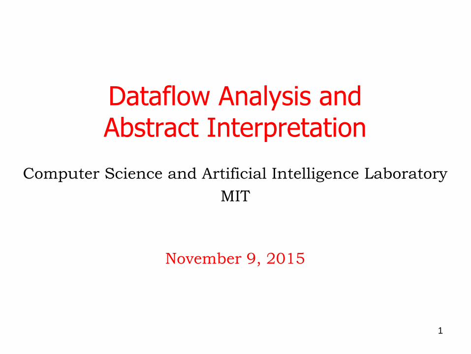
o Last time we developed from first principles an algorithm

to derive invariants.

o Key idea:

- Define a lattice of possible invariants

- Define a fixpoint equation whose solution will give you the

invariants

o Today we follow a more historical development and will

present a formalization that will allow us to better reason

about this kind of analysis algorithms

2

Dataflow Analysis

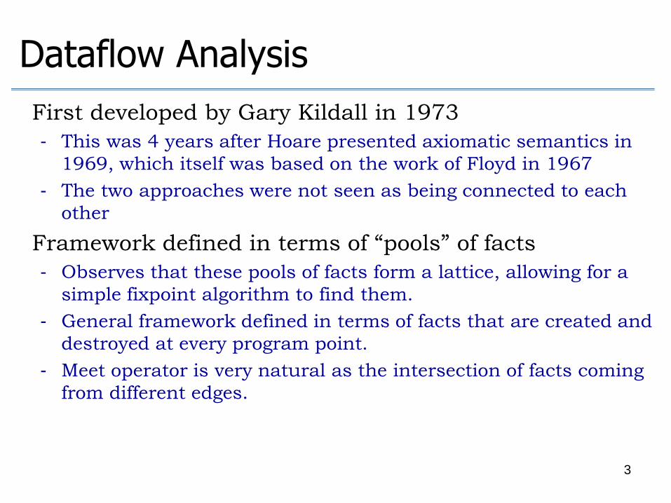
o First developed by Gary Kildall in 1973

- This was 4 years after Hoare presented axiomatic semantics in

1969, which itself was based on the work of Floyd in 1967

- The two approaches were not seen as being connected to each

other

o Framework defined in terms of “pools” of facts

- Observes that these pools of facts form a lattice, allowing for a

simple fixpoint algorithm to find them.

- General framework defined in terms of facts that are created and

destroyed at every program point.

- Meet operator is very natural as the intersection of facts coming

from different edges.

3

Forward Dataflow Analysis

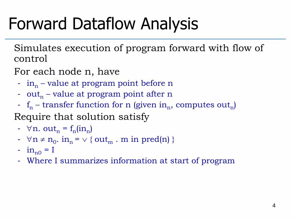
o Simulates execution of program forward with flow of control

o For each node n, have - inn – value at program point before n

- outn – value at program point after n

- fn – transfer function for n (given inn, computes outn)

o Require that solution satisfy - n. outn = fn(inn)

- n n0. inn = { outm . m in pred(n) }

- inn0 = I

- Where I summarizes information at start of program

4

Dataflow Equations

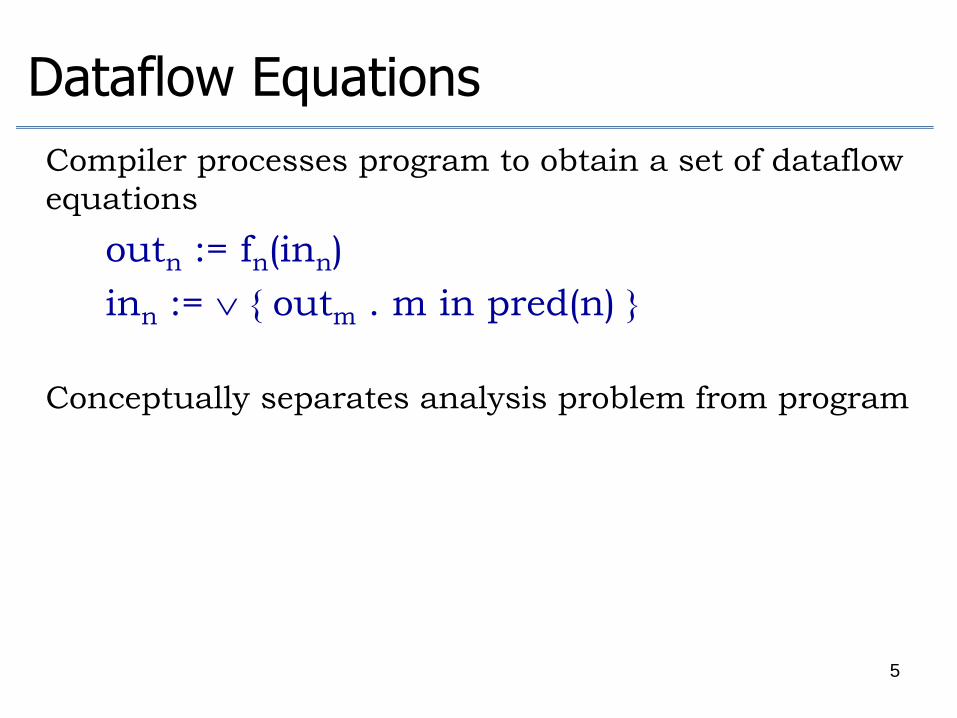
o Compiler processes program to obtain a set of dataflow

equations

outn := fn(inn)

inn := { outm . m in pred(n) }

o Conceptually separates analysis problem from program

5

Worklist Algorithm for Solving Forward Dataflow Equations

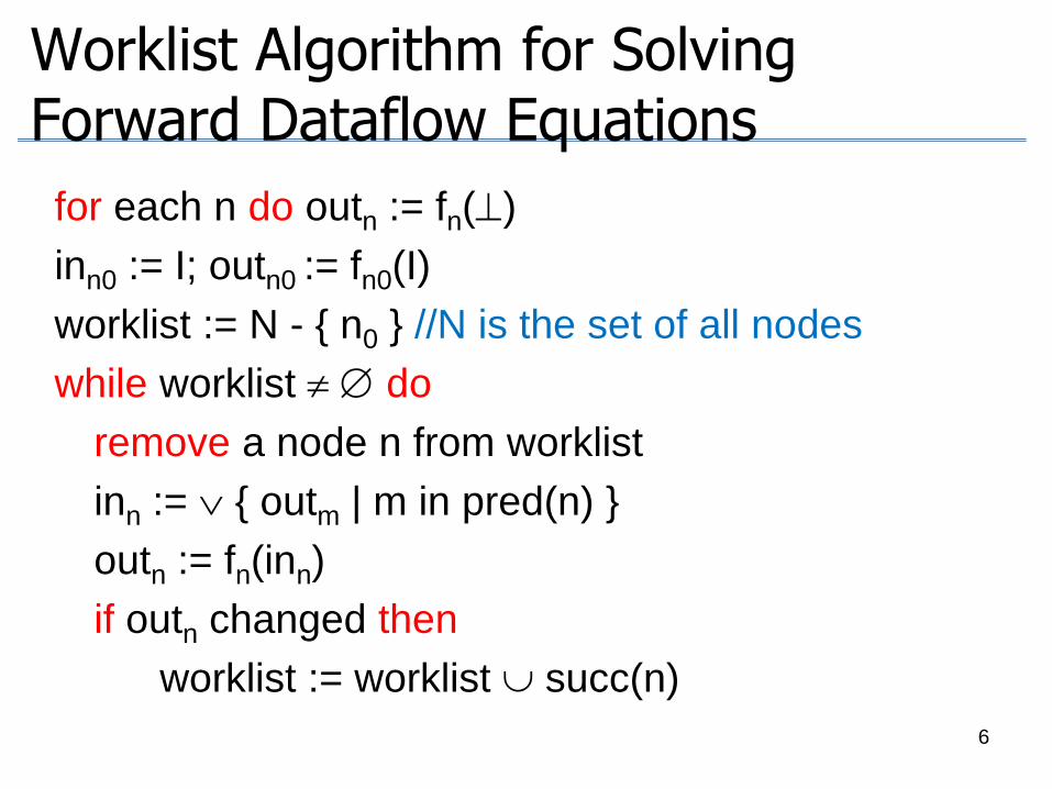
for each n do outn := fn()

inn0 := I; outn0 := fn0(I)

worklist := N - { n0 } //N is the set of all nodes

while worklist do

remove a node n from worklist

inn := { outm | m in pred(n) }

outn := fn(inn)

if outn changed then

worklist := worklist succ(n)

6

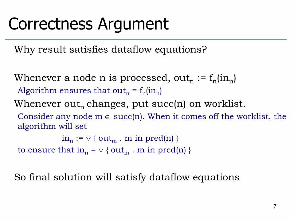
Correctness Argument

o Why result satisfies dataflow equations?

o Whenever a node n is processed, outn := fn(inn)

Algorithm ensures that outn = fn(inn)

o Whenever outn changes, put succ(n) on worklist.

Consider any node m succ(n). When it comes off the worklist, the

algorithm will set

inn := { outm . m in pred(n) }

to ensure that inn = { outm . m in pred(n) }

o So final solution will satisfy dataflow equations

7

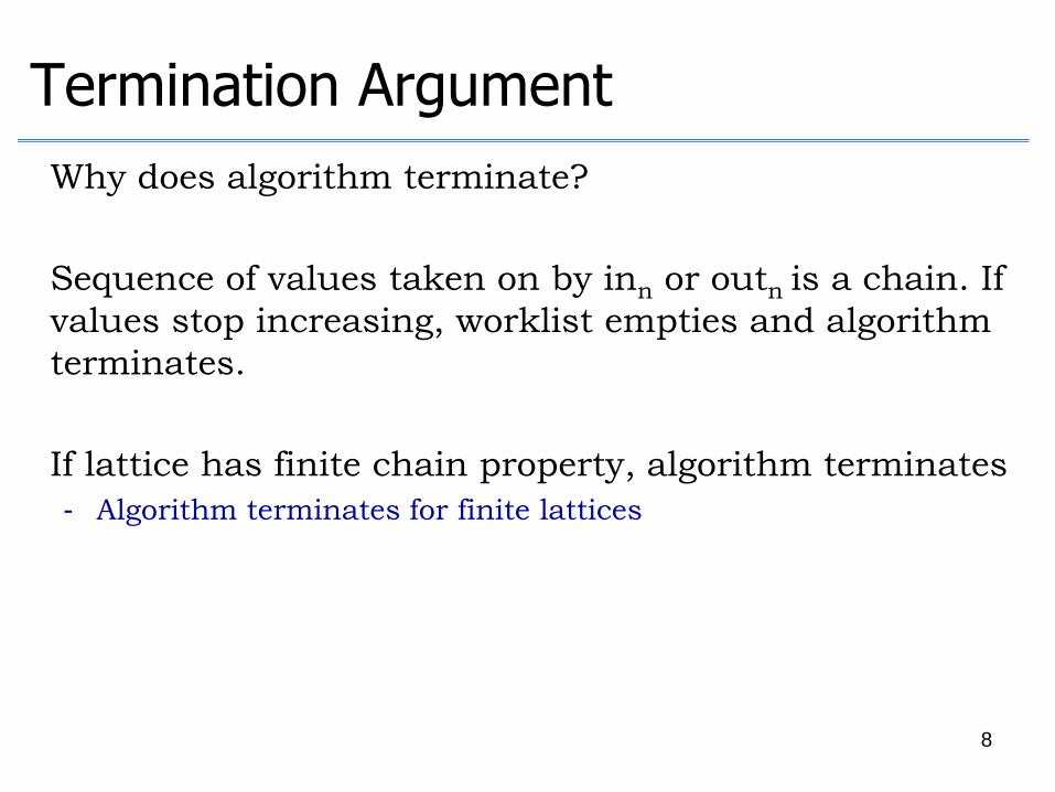
Termination Argument

o Why does algorithm terminate?

o Sequence of values taken on by inn or outn is a chain. If

values stop increasing, worklist empties and algorithm

terminates.

o If lattice has finite chain property, algorithm terminates

- Algorithm terminates for finite lattices

8

Abstract Interpretation

15

History

o POPL 77 paper by Patrick Cousot and Radhia Cousot

- Brings together ideas from the compiler optimization community

with ideas in verification

- Provides a clean and general recipe for building analyses and

reasoning about their correctness

16

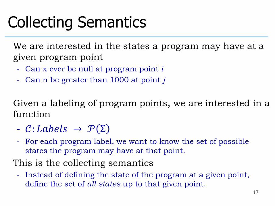
Collecting Semantics

o We are interested in the states a program may have at a

given program point

- Can x ever be null at program point i

- Can n be greater than 1000 at point j

o Given a labeling of program points, we are interested in a

function

- 𝒞: 𝐿𝑎𝑏𝑒𝑙𝑠 → 𝒫 Σ - For each program label, we want to know the set of possible

states the program may have at that point.

o This is the collecting semantics

- Instead of defining the state of the program at a given point,

define the set of all states up to that given point. 17

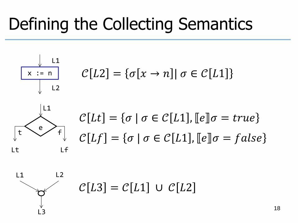
Defining the Collecting Semantics

x := n

L1

L2

𝒞 𝐿2 = 𝜎 𝑥 → 𝑛 | 𝜎 ∈ 𝒞 𝐿1

e t f

Lt Lf

L1

𝒞 𝐿𝑡 = 𝜎 | 𝜎 ∈ 𝒞 𝐿1 , 𝑒 𝜎 = 𝑡𝑟𝑢𝑒

𝒞 𝐿𝑓 = 𝜎 | 𝜎 ∈ 𝒞 𝐿1 , 𝑒 𝜎 = 𝑓𝑎𝑙𝑠𝑒

L1 L2

L3

𝒞 𝐿3 = 𝒞 𝐿1 ∪ 𝒞 𝐿2

18

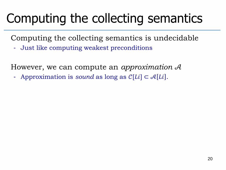
Computing the collecting semantics

o Computing the collecting semantics is undecidable

- Just like computing weakest preconditions

o However, we can compute an approximation 𝒜

- Approximation is sound as long as 𝒞[𝐿𝑖] ⊂ 𝒜 𝐿𝑖 .

20

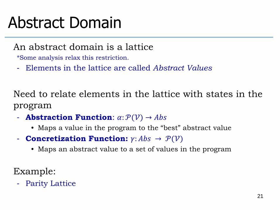
Abstract Domain

o An abstract domain is a lattice *Some analysis relax this restriction.

- Elements in the lattice are called Abstract Values

o Need to relate elements in the lattice with states in the

program

- Abstraction Function: 𝛼: 𝒫(𝒱) → 𝐴𝑏𝑠

• Maps a value in the program to the “best” abstract value

- Concretization Function: 𝛾: 𝐴𝑏𝑠 → 𝒫(𝒱)

• Maps an abstract value to a set of values in the program

o Example:

- Parity Lattice

21

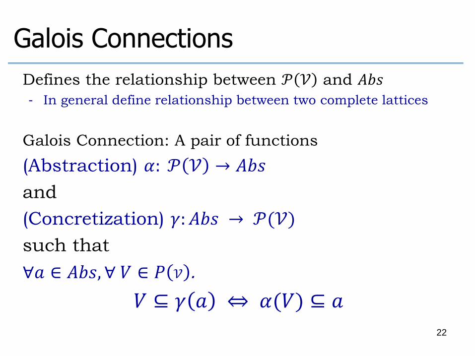
Galois Connections

o Defines the relationship between 𝒫 𝒱 and 𝐴𝑏𝑠

- In general define relationship between two complete lattices

o Galois Connection: A pair of functions

o (Abstraction) 𝛼: 𝒫 𝒱 → 𝐴𝑏𝑠

o and

o (Concretization) 𝛾: 𝐴𝑏𝑠 → 𝒫(𝒱)

o such that

o ∀𝑎 ∈ 𝐴𝑏𝑠, ∀ 𝑉 ∈ 𝑃 𝒱 .

o 𝑉 ⊆ 𝛾 𝑎 ⇔ 𝛼(𝑉) ⊆ 𝑎

22

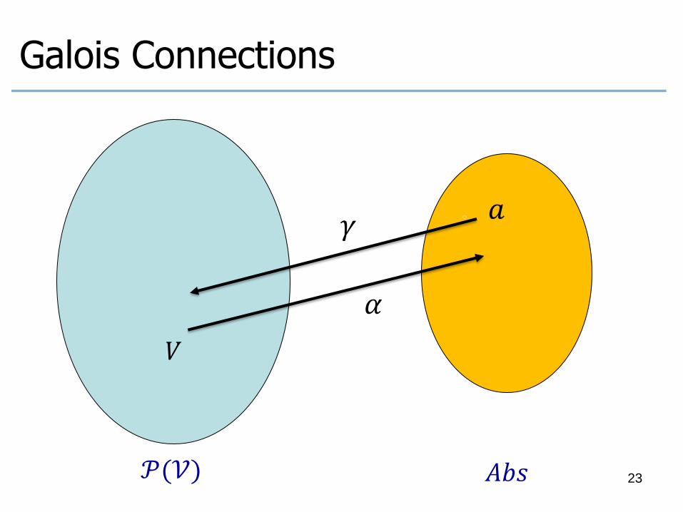
Galois Connections

o 𝒫(𝒱) 𝐴𝑏𝑠

𝛾

𝛼

𝑉

o 𝑎

23

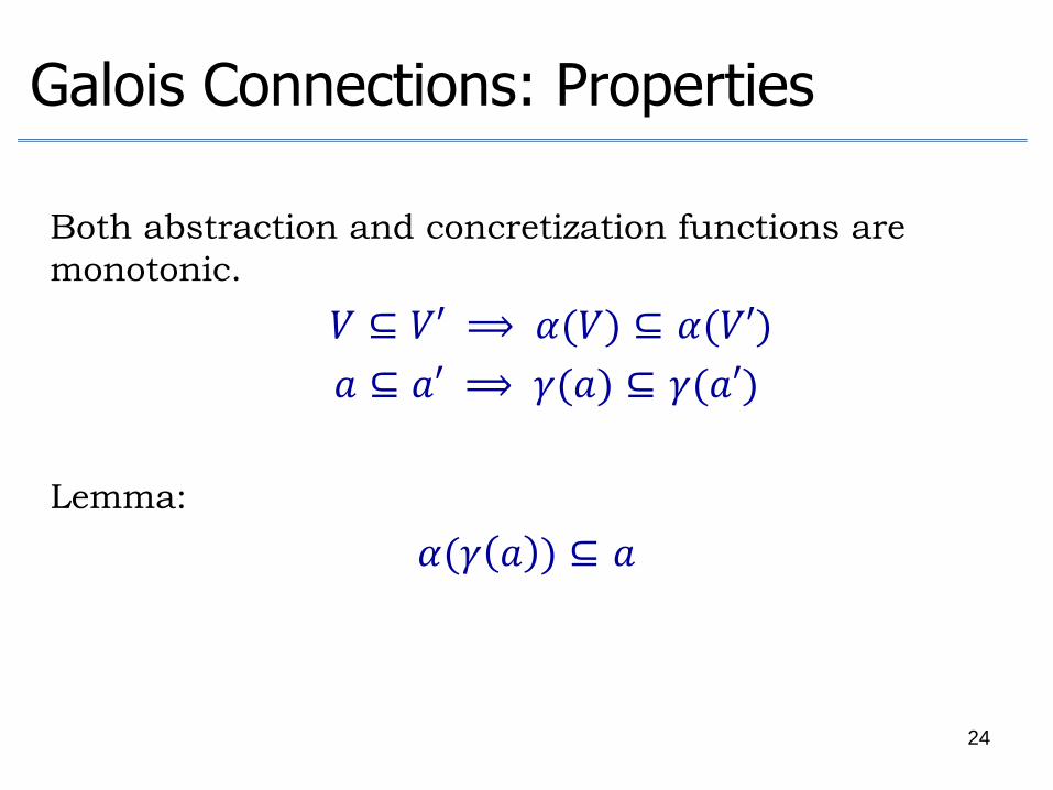
Galois Connections: Properties

o Both abstraction and concretization functions are

monotonic.

o 𝑉 ⊆ 𝑉′ ⟹ 𝛼(𝑉) ⊆ 𝛼(𝑉′)

o 𝑎 ⊆ 𝑎′ ⟹ 𝛾(𝑎) ⊆ 𝛾(𝑎′)

o Lemma:

𝛼(𝛾 𝑎 ) ⊆ 𝑎

24

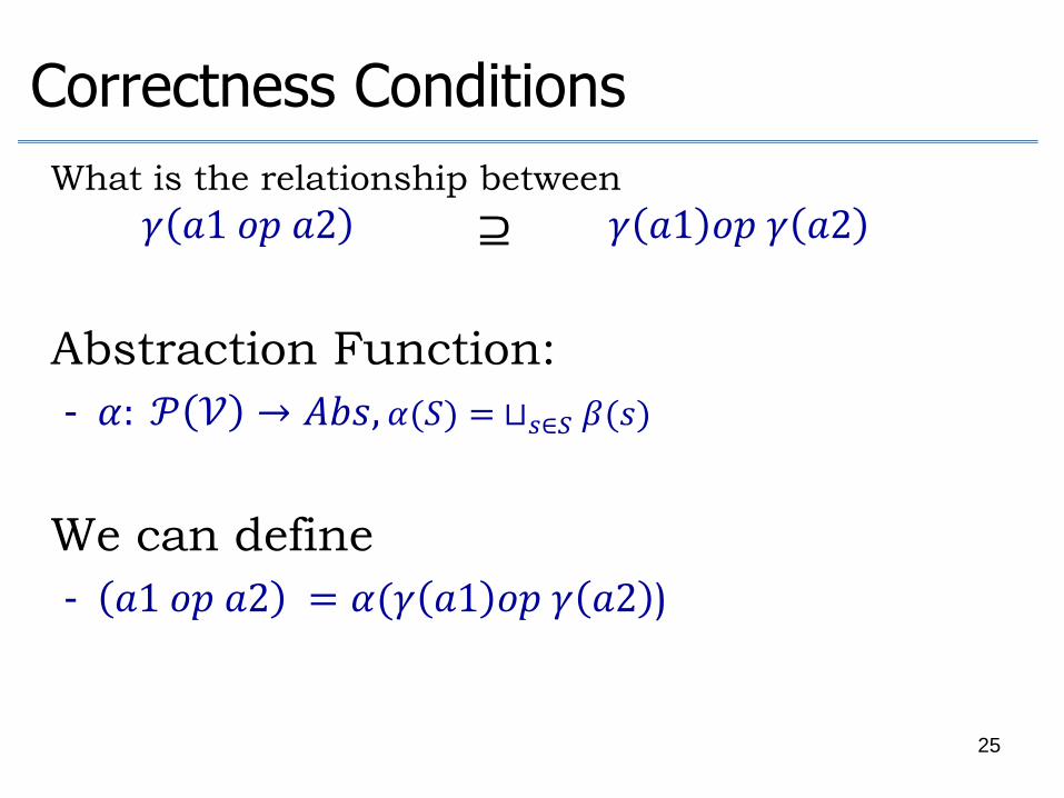
Correctness Conditions

o What is the relationship between

𝛾 𝑎1 𝑜𝑝 𝑎2 𝛾 𝑎1 𝑜𝑝 𝛾 𝑎2

o Abstraction Function:

- 𝛼: 𝒫 𝒱 → 𝐴𝑏𝑠, 𝛼(𝑆) = ⊔𝑠∈𝑆 𝛽(𝑠)

o We can define - 𝑎1 𝑜𝑝 𝑎2 = 𝛼(𝛾 𝑎1 𝑜𝑝 𝛾 𝑎2 )

⊇

25

Abstract Domains: Examples

- Constant domain

- Sign domain

- Interval domain

26

Abstract Interpretation

o Simple recipe for arguing correctness of an analysis

- Define an abstract domain Abs

- Define 𝛼 and 𝛾 and show they form a Gallois

Connection

- Define the semantics of program constructs for the

abstract domain and show that they are correct

27

Some useful domains

o Ranges

- Useful for detecting out-of-bounds errors, potential overflows

o Linear relationships between variables

- 𝑎1𝑥1 + 𝑎2𝑥2 + ⋯ + 𝑎𝑘𝑥𝑘 ≥ 𝑐

o Problem: Both of these domains have infinite chains!

28

Widening

o Key idea:

- You have been running your analysis for a while

- A value keeps getting “bigger” and “bigger” but refuses to

converge

- Just declare it to be ⊤ (or some other big value)

o This loses precision

- but it’s always sound

o Widening operator: 𝛻: 𝐴𝑏𝑠 × 𝐴𝑏𝑠 → 𝐴𝑏𝑠

- 𝑎1 𝛻 𝑎2 ⊒ 𝑎1, 𝑎2

29

MIT OpenCourseWarehttp://ocw.mit.edu

6.820 Fundamentals of Program AnalysisFall 2015

For information about citing these materials or our Terms of Use, visit: http://ocw.mit.edu/terms.