Database Management System Support for Collaborative ...

Database Management System Support for CollaborativeFiltering Recommender Systems

A THESIS

SUBMITTED TO THE FACULTY OF THE GRADUATE SCHOOL

OF THE UNIVERSITY OF MINNESOTA

BY

Mohamed Sarwat

IN PARTIAL FULFILLMENT OF THE REQUIREMENTS

FOR THE DEGREE OF

DOCTOR OF PHILOSOPHY, PhD

Mohamed F. Mokbel

August, 2014

c© Mohamed Sarwat 2014

ALL RIGHTS RESERVED

Acknowledgements

There are many people that have earned my gratitude for their contribution to my

time in graduate school. More specifically, I would like to thank five groups of people,

without whom this thesis would not have been possible: my thesis committee members,

my lab mates, my industrial collaborators, funding agencies, and my family.

First, I am indebted to my thesis advisor, Mohamed F. Mokbel. Since my first

day in graduate school, Mohamed believed in me like nobody else and gave me endless

support. It all started in Fall 2009 when he offered me such a great opportunity to join

the data management lab. On the academic level, Mohamed taught me fundamentals

of conducting scientific research in the database systems area. Under his supervision, I

learned how to define a research problem, find a solution to it, and finally publish the

results. On a personal level, Mohamed inspired me by his hardworking and passionate

attitude. To summarize, I would give Mohamed most of the credit for becoming the

kind of scientist I am today.

Besides my advisor, I would like to thank the rest of my dissertation committee mem-

bers (Gedas Adocmivicius, Shashi Shekhar, and Eric Van Wyk) for their great support

and invaluable advice. I am thankful to Prof. Adomavicius, an expert in context-aware

recommender systems, for his crucial remarks that shaped my final dissertation. I am

also grateful to Prof. Shekhar for his insightful comments and for sharing with me his

tremendous experience in the spatial data management field. I am quite appreciative

of Prof. Eric Van Wyk for agreeing to serve on my dissertation committee on such

a short notice as a replacement for John Riedl. I also show gratitude for Prof. John

Riedl (former thesis committee member), an excellent teacher and pioneer in the recom-

mender systems area, who unfortunately passed away a few months before the official

dissertation defense.

i

I would like to thank my lab mates for their continued support. This dissertation

would not have been possible without the intellectual contribution of Justin J. Levan-

doski, a data management lab alumni. Moreover, I am thankful to James Avery and

Ahmed Eldawy for their collaboration and contribution in various projects related to this

dissertation. I would also like to thank my other lab mates that include Louai Alarabi,

Jie Bao, Chi-Yin Chow, Abdeltawab Hendawi, Mohamed Khalefa, Amr Magdy, and

Joe Naps for making my experience in the data management lab and graduate school

exciting and fun.

I am also grateful to my industrial collaborators. I spent two summers at Microsoft

Research where I had the chance to collaborate with fantastic researchers. More specifi-

cally, I would like to thank Sameh Elnikety and Yuxiong He for their continuous support

and for providing me the great opportunity to work on large-scale systems. I also extend

my gratitude to members of the database, cloud systems, and DMX groups at Microsoft

research for the fruitful discussions and for making my internship at Microsoft such an

eye-opening experience. I also had one summer internship at NEC laboratories where

I have collaborated with wonderful scientists in the Data Management department. I

would like to thank Jagan Sankaranarayanan (my mentor at NEC Labs) and Hakan

Hacigumus (my manager at NEC Labs) for their great mentorship and guidance.

Thanks are also due to the (NSF) National Science Foundation (under Grants IIS-

0952977, IIS-1218168, IIS-0811998, IIS-0811935, and CNS-0708604), University of Min-

nesota Digital Technology Center, and Microsoft Research for their financial support

that I otherwise would not have been able to develop my scientific discoveries.

Last but not least, I would like to express my deepest gratitude to my family and

friends. This dissertation would not have been possible without their warm love, con-

tinued patience, and endless support.

ii

Dedication

I dedicate this thesis to my beloved son Yossuf.

iii

Abstract

Recommender systems help users identify useful, interesting items or content (data)

from a considerably large search space. By far, the most popular recommendation

technique used is collaborative filtering which exploits the users’ opinions (e.g., movie

ratings) and/or purchasing (e.g., watching, reading) history in order to extract a set

of interesting items for each user. Database Management Systems (DBMSs) do not

provide in-house support for recommendation applications despite their popularity. Ex-

isting recommender system architectures either do not employ a DBMS at all or only

uses it as a data store whereas the recommendation logic is implemented in-full outside

the database engine. Incorporating the recommendation functionality inside the DBMS

kernel is beneficial for the following reasons: (1) Many recommendation algorithms take

as input structured data (users, items, and user historical preferences) that could be

adequately stored and accessed using a database system. (2) The In-DBMS approach

facilitates applying the recommendation functionality and typical database operations

(e.g., Selection, Join) side-by-side. That allows application developers to go beyond

traditional recommendation applications, e.g., “Recommend to Alice ten movies”, and

flexibly define Arbitrary Recommendation scenarios like “Recommend ten nearby restau-

rants to Alice” and “Recommend to Bob ten movies watched by her friends”. (3) Once

the recommendation functionality lives inside the database kernel, the recommendation

application takes advantage of the DMBS inherent features (e.g., query optimization,

materialized views, indexing) provided by the storage manager and query execution en-

gine. This thesis studies the incorporation of the recommendation functionality inside

the core engine of a database management system. This is a major departure from

existing recommender system architectures that are implemented on-top of a database

engines using either SQL queries or stored procedures. The on-top approach does not

harness the full power of the database engine (i.e., query execution engine, storage man-

ager) since it always generates recommendations first and then performs other database

operations. Ideas developed in this thesis are implemented inside RecDB ; an open-

source recommendation engine built entirely inside PostgreSQL (open source relational

database system).

iv

Contents

Acknowledgements i

Dedication iii

Abstract iv

List of Tables vi

List of Figures vii

1 Introduction 1

1.1 Recommender Systems . . . . . . . . . . . . . . . . . . . . . . . . . . . . 1

1.2 Database Management Systems . . . . . . . . . . . . . . . . . . . . . . . 2

1.3 Contribution and Organization . . . . . . . . . . . . . . . . . . . . . . . 3

2 Recommender Systems and Databases 6

2.1 Collaborative Filtering . . . . . . . . . . . . . . . . . . . . . . . . . . . . 7

2.1.1 Offline Model Generation . . . . . . . . . . . . . . . . . . . . . . 8

2.1.2 Online recommendation generation . . . . . . . . . . . . . . . . . 10

2.2 DBMS-based Collaborative Filtering . . . . . . . . . . . . . . . . . . . . 11

3 Database Support for Recommender Systems 15

3.1 RecDB Overview . . . . . . . . . . . . . . . . . . . . . . . . . . . . . . . 15

3.2 Using RecDB . . . . . . . . . . . . . . . . . . . . . . . . . . . . . . . . . 17

3.2.1 Creating a Recommender . . . . . . . . . . . . . . . . . . . . . . 18

3.2.2 Updating a Recommender . . . . . . . . . . . . . . . . . . . . . . 20

v

3.2.3 Querying a Recommender . . . . . . . . . . . . . . . . . . . . . . 20

3.3 Case Studies . . . . . . . . . . . . . . . . . . . . . . . . . . . . . . . . . 21

3.3.1 Movie Recommendation . . . . . . . . . . . . . . . . . . . . . . . 21

3.3.2 Point-of-Interest (POI) Recommendation . . . . . . . . . . . . . 22

4 Online Recommendation Model Maintenance 26

4.1 RecStore Architecture . . . . . . . . . . . . . . . . . . . . . . . . . . . . 28

4.2 RecStore: Built-In Online DBMS-Based Recommenders . . . . . . . . . 29

4.2.1 Online Model Maintenance . . . . . . . . . . . . . . . . . . . . . 29

4.2.2 Adaptive Strategies for System Workloads . . . . . . . . . . . . . 31

4.3 RecStore Extensibility . . . . . . . . . . . . . . . . . . . . . . . . . . . . 35

4.3.1 Registering a Recommender algorithm . . . . . . . . . . . . . . . 36

4.3.2 Item-Based Collaborative Filtering . . . . . . . . . . . . . . . . . 36

4.3.3 User-based Collaborative Filtering . . . . . . . . . . . . . . . . . 39

4.3.4 Non-“neighborhood-based” Collaborative Filtering within RecStore 39

4.4 Experimental Evaluation . . . . . . . . . . . . . . . . . . . . . . . . . . . 40

4.4.1 Hotspot Detection Strategies . . . . . . . . . . . . . . . . . . . . 40

4.4.2 Update Efficiency . . . . . . . . . . . . . . . . . . . . . . . . . . . 42

4.4.3 Query Efficiency . . . . . . . . . . . . . . . . . . . . . . . . . . . 42

4.4.4 Update + Query Workload . . . . . . . . . . . . . . . . . . . . . 43

5 Recommendation Query Processing and Optimization 46

5.1 Recommendation Operators . . . . . . . . . . . . . . . . . . . . . . . . . 47

5.1.1 Item-Item Collaborative Filtering Operator . . . . . . . . . . . . 48

5.1.2 User-User Collaborative Filtering Operator . . . . . . . . . . . . 49

5.1.3 Matrix Factorization Operator . . . . . . . . . . . . . . . . . . . 50

5.2 Query Pipeline Integration . . . . . . . . . . . . . . . . . . . . . . . . . . 51

5.2.1 Selection . . . . . . . . . . . . . . . . . . . . . . . . . . . . . . . 51

5.2.2 Join . . . . . . . . . . . . . . . . . . . . . . . . . . . . . . . . . . 53

5.2.3 Ranking . . . . . . . . . . . . . . . . . . . . . . . . . . . . . . . . 53

5.3 Optimization Strategies . . . . . . . . . . . . . . . . . . . . . . . . . . . 54

5.3.1 Selection Optimization . . . . . . . . . . . . . . . . . . . . . . . . 55

5.3.2 Join Optimization . . . . . . . . . . . . . . . . . . . . . . . . . . 56

vi

5.3.3 Optimization through Pre-Computation . . . . . . . . . . . . . . 56

5.3.4 Scalability . . . . . . . . . . . . . . . . . . . . . . . . . . . . . . . 58


5.4.1 Recommender Queries . . . . . . . . . . . . . . . . . . . . . . . . 63

5.4.2 Recommender Storage and Maintenance . . . . . . . . . . . . . . 68

6 RecDB Support for Context Pre-filtering Recommenders 69

6.1 Context Pre-Filtering Recommender . . . . . . . . . . . . . . . . . . . . 70

6.1.1 Creating a Recommender . . . . . . . . . . . . . . . . . . . . . . 70

6.1.2 Querying a Recommender . . . . . . . . . . . . . . . . . . . . . . 71

6.2 Data Structure . . . . . . . . . . . . . . . . . . . . . . . . . . . . . . . . 72

6.2.1 Recommender Catalog . . . . . . . . . . . . . . . . . . . . . . . . 73

6.2.2 Recommender Grid . . . . . . . . . . . . . . . . . . . . . . . . . . 73

6.2.3 The CFilter Function . . . . . . . . . . . . . . . . . . . . . . . . 74


7 Handling Location-Aware Recommendation Scenarios 78

7.1 A Study of Location-Based Ratings . . . . . . . . . . . . . . . . . . . . . 79

7.2 Non-Spatial User Ratings for Non-Spatial Items . . . . . . . . . . . . . . 80

7.3 Spatial User Ratings for Non-Spatial Items . . . . . . . . . . . . . . . . 80

7.3.1 Data Structure . . . . . . . . . . . . . . . . . . . . . . . . . . . . 81

7.3.2 Query Processing . . . . . . . . . . . . . . . . . . . . . . . . . . . 82

7.3.3 Data Structure Maintenance . . . . . . . . . . . . . . . . . . . . 83

7.3.4 Partial Merging and Splitting . . . . . . . . . . . . . . . . . . . . 90

7.4 Optimized Spatial User Ratings for Non-Spatial Items . . . . . . . . . . 91

7.4.1 Pyramid structure intuition . . . . . . . . . . . . . . . . . . . . . 92

7.4.2 LARS* versus LARS . . . . . . . . . . . . . . . . . . . . . . . . . 94

7.4.3 Pyramid Maintenance . . . . . . . . . . . . . . . . . . . . . . . . 95

7.5 Non-Spatial User Ratings for Spatial Items . . . . . . . . . . . . . . . . 104

7.5.1 Query Processing . . . . . . . . . . . . . . . . . . . . . . . . . . . 105

7.5.2 Incremental Travel Penalty Computation . . . . . . . . . . . . . 106

7.6 Spatial User Ratings for Spatial Items . . . . . . . . . . . . . . . . . . . 108


vii

7.7.1 Recommendation Quality for Varying Pyramid Levels . . . . . . 110

7.7.2 Recommendation Quality for Varying k . . . . . . . . . . . . . . 113

7.7.3 Recommendation Quality for VaryingM . . . . . . . . . . . . . 113

7.7.4 Storage Vs. Locality . . . . . . . . . . . . . . . . . . . . . . . . . 114

7.7.5 Scalability . . . . . . . . . . . . . . . . . . . . . . . . . . . . . . . 115

7.7.6 Query Processing Performance . . . . . . . . . . . . . . . . . . . 116

8 Related Work 119

9 Conclusion and Discussion 123

9.1 Summary . . . . . . . . . . . . . . . . . . . . . . . . . . . . . . . . . . . 123

9.2 Future Directions . . . . . . . . . . . . . . . . . . . . . . . . . . . . . . . 125

References 127

viii

List of Tables

4.1 Realizing probabilistic and Pearson item-based collaborative filtering . . 37

5.1 Materialization Manager Example . . . . . . . . . . . . . . . . . . . . . 61

7.1 Comparison between LARS and LARS* . . . . . . . . . . . . . . . . . . . . 95

7.2 Summary of Mathematical Notations. . . . . . . . . . . . . . . . . . . . . . 99

ix

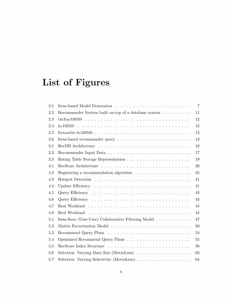
List of Figures

2.1 Item-based Model Generation . . . . . . . . . . . . . . . . . . . . . . . . 7

2.2 Recommender System built on-top of a database system . . . . . . . . . 11

2.3 OnTop-DBMS . . . . . . . . . . . . . . . . . . . . . . . . . . . . . . . . . 12

2.4 In-DBMS . . . . . . . . . . . . . . . . . . . . . . . . . . . . . . . . . . . . 12

2.5 Extensible In-DBMS . . . . . . . . . . . . . . . . . . . . . . . . . . . . . . 12

2.6 Item-based recommender query . . . . . . . . . . . . . . . . . . . . . . . 13

3.1 RecDB Architecture . . . . . . . . . . . . . . . . . . . . . . . . . . . . . 16

3.2 Recommender Input Data. . . . . . . . . . . . . . . . . . . . . . . . . . . 17

3.3 Rating Table Storage Representation . . . . . . . . . . . . . . . . . . . . 19

4.1 RecStore Architecture . . . . . . . . . . . . . . . . . . . . . . . . . . . . 29

4.2 Registering a recommendation algorithm . . . . . . . . . . . . . . . . . . 35

4.3 Hotspot Detection . . . . . . . . . . . . . . . . . . . . . . . . . . . . . . 41

4.4 Update Efficiency . . . . . . . . . . . . . . . . . . . . . . . . . . . . . . . 41

4.5 Query Efficiency . . . . . . . . . . . . . . . . . . . . . . . . . . . . . . . 43

4.6 Query Efficiency . . . . . . . . . . . . . . . . . . . . . . . . . . . . . . . 43

4.7 Real Workload . . . . . . . . . . . . . . . . . . . . . . . . . . . . . . . . 44

4.8 Real Workload . . . . . . . . . . . . . . . . . . . . . . . . . . . . . . . . 44

5.1 Item-Item (User-User) Collaborative Filtering Model . . . . . . . . . . . 47

5.2 Matrix Factorization Model . . . . . . . . . . . . . . . . . . . . . . . . . 50

5.3 Recommend Query Plans . . . . . . . . . . . . . . . . . . . . . . . . . . 54

5.4 Optimized Recommend Query Plans . . . . . . . . . . . . . . . . . . . . 55

5.5 RecScore Index Structure . . . . . . . . . . . . . . . . . . . . . . . . . . 56

5.6 Selection: Varying Data Size (MovieLens) . . . . . . . . . . . . . . . . . 63

5.7 Selection: Varying Selectivity (MovieLens) . . . . . . . . . . . . . . . . . 64

x

5.8 Join: Joined Recommender Data Size (Foursquare) . . . . . . . . . . . . 65

5.9 Join: Joined Table (rel) Selectivity (Foursquare) . . . . . . . . . . . . . 65

5.10 Ranking: Varying Data Size (MovieLens) . . . . . . . . . . . . . . . . . 66

5.11 Ranking: Varying Limit (k) Size (MovieLens) . . . . . . . . . . . . . . . 66

5.12 Scalability Vs. Queries (SVD) (MovieLens) . . . . . . . . . . . . . . . . 67

5.13 Scalability Vs. Queries (ItemCosCF) (MovieLens) . . . . . . . . . . . . 68

6.1 Recommender Grid data structure . . . . . . . . . . . . . . . . . . . . . 72

6.2 Initialization Time and Storage Overhead. . . . . . . . . . . . . . . . . . 76

7.1 Preference locality in location-based ratings. . . . . . . . . . . . . . . . . 79

7.2 Partial pyramid data structure. . . . . . . . . . . . . . . . . . . . . . . . 82

7.3 Merge and split example . . . . . . . . . . . . . . . . . . . . . . . . . . . 87

7.4 Example of Items Ratings Statistics Table . . . . . . . . . . . . . . . . . . . 92

7.5 Two-Levels Pyramid . . . . . . . . . . . . . . . . . . . . . . . . . . . . . . 92

7.6 Ratings Distribution and Recommendation Models . . . . . . . . . . . . . . 93

7.7 Locality Loss/Gain at Cp] . . . . . . . . . . . . . . . . . . . . . . . . . . . 94

7.8 Quality experiments for varying locality . . . . . . . . . . . . . . . . . . . . 111

7.9 Quality experiments for varying answer sizes . . . . . . . . . . . . . . . . . . 112

7.10 Quality experiments for varying value ofM . . . . . . . . . . . . . . . . . . 114

7.11 Effect ofM on storage and locality (Synthetic data) . . . . . . . . . . . . . . 115

7.12 Scalability of the adaptive pyramid (Synthetic data) . . . . . . . . . . . . . . 116

7.13 Query Processing Performance (Synthetic data). . . . . . . . . . . . . . . . . 117

xi

Chapter 1

Introduction

1.1 Recommender Systems

”What end-users really want?” a question asked by almost every business, online retail

store, or content provider. The answer to this question helps users find interesting items

(e.g., products, movies, books). In a pursuit to such an answer, researchers have been

crafting novel technologies that provide a personalized experience to end-users. Among

such technologies, recommender systems have been widely used in both industry [1, 2,

3, 4] and academia [5, 6, 7, 8, 9, 10, 11, 12]. The purpose of recommender systems is to

help users identify useful, interesting items or content (data) from a considerably large

search space. For example, recommender systems have successfully been used to help

users find interesting books and media from a massive inventory base in Amazon [4],

movies from a large catalog in Netflix [13] and Movielens [9], TV programs from TV

Genuis [14], college courses in CourseRank [15], or even food from Freshdirect [16],

among other applications.

A recommender system exploits the users’ opinions (e.g., movie ratings) and/or

purchasing (e.g., watching, reading) history in order to extract a set of interesting

items for each user. Collaborative filtering [6, 17, 18, 19, 20, 21] comes as one of

the most popular recommendation methods proposed in the literature. Collaborative

filtering recommendation algorithms consist of two main phases: (1) A computationally

expensive offline model generation phase that uses community opinions (i.e., user rating

triples represented as (user, item, rating)) in order to derive meaningful correlations

1

2

between users or items, and (2) An online recommendation generation phase that uses

the model to produce recommendations.

With its wide use, recommender systems have been mostly applied only to, now

classical, web applications of retail stores (e.g., Amazon and Netflix) that manage to

have somehow static set of objects that are infrequently updated. In such applications,

the recommendation changes very slowly over time [22, 21]. Hence, it is enough to peri-

odically (e.g., weekly) rerun the offline model generation phase. The scope of most work

within recommender systems has been from a user-centric perspective, e.g., providing

users with quality [17, 23] and trustworthy recommendations [24]. There is a scarcity

of work that studies recommenders from a systems perspective, i.e., measuring query

processing efficiency of different architectures. Herlocker et al. in their 2004 detailed

evaluation of recommender systems state [17]:

“We have chosen not to discuss computation performance of recommender algo-

rithms. Such performance is certainly important, and in the future we expect there to

be work on the quality of time-limited and memory-limited recommendations.”

We are living in the era of staggering web use growth and ever-popular social media

applications (e.g., Facebook [25], Twitter [26]) where: (a) users are expressing their

opinions over a diverse set of items (e.g., Facebook “likes”) faster than ever. Hence,

weeks, days, or even hours to rebuild the recommendation model is not acceptable [3],

(b) there is an urge need to support arbitrary recommendations that do not only fit

the prior user ratings, but also fit the user profile and context, e.g., context-aware

recommender systems [33, 34, 35, 36], and (c) users and items spatial locations play a

major role in the quality of the recommendation result as has been indicated by New

York times [27] and Foursqaure [28] as well as various academic studies [29, 30, 31, 32].

1.2 Database Management Systems

A Database is a collection of data that typically describes entities and interactions

among these entities, e.g., flight reservations, product purchases, student grades, part

inventory system. A Database Management System (DBMS) is a software artifact that

enables storing, maintaining, and accessing data efficiently [37]. For more than four

decades, DBMSs have been a major contributor to the information technology world.

3

A modern DBMS consists of two main modules: (1) A storage manager that adopts a

suitable storage layout to physically represent the data, stores the data on a persistent

storage medium, and provides efficient access methods for the stored data. (2) A query

execution engine that parses the incoming query, optimizes it into an execution plan,

and finally executes the query.

DBMSs do not provide in-house support for recommendation applications despite

their popularity. Existing recommender system architectures either do not employ

a DBMS at all or only use it as a data store whereas the recommendation logic is

implemented in-full outside the database engine. Incorporating the recommendation

functionality inside the DBMS kernel is beneficial for the following reasons: (1) Many

recommendation algorithms take as input structured data (e.g., users, items, and user

historical preferences) that could be adequately stored and accessed using a database

management system. Recent work from the data management community has shown

that many popular recommendation methods (including collaborative filtering) can be

expressed with conventional SQL, effectively pushing the core logic of recommender sys-

tems within the database management system (DBMS) [38]. (2) The In-DBMS approach

facilitates applying the recommendation functionality and typical database operations

(e.g., Selection, Join) side-by-side. That allows application developers to go beyond

traditional recommendation applications, e.g., “Recommend to Alice ten movies”, and

flexibly define Arbitrary Recommendation scenarios like “Recommend ten nearby restau-

rants to Alice” and “Recommend to Bob ten movies watched by her friends”. (3) Once

the recommendation functionality lives inside the database kernel, the recommendation

application takes advantage of the DMBS inherent features (e.g., query optimization,

materialized views, indexing) provided by the storage manager and query execution

engine.

1.3 Contribution and Organization

The overarching goal of this thesis is to conduct research, develop requisite knowledge

to advance the state-of-the-art and usage of recommender systems. This thesis is the

first of its kind to study the integration of both the recommender system and database

management system. Given this outlook, this document is organized as follows:

4

• Chapter 2 gives an overview of collaborative filtering recommenders and ana-

lyzes the straightforward approach of implementing a collaborative filtering rec-

ommender using a database management system.

• Chapter 3 presents the architecture of RecDB ; an In-DBMS recommender sys-

tem that incorporates the recommendation functionality inside the database ker-

nel. This chapter also explains RecDB ’s SQL interface for creating and querying

recommenders as well as describes two RecDB case studies (i.e., Movie Recom-

mendation, Point-of-Interest Recommendation).

• Online updates come from new or deleted items (e.g., news item, microblog en-

tries) or ratings (e.g., Facebook likes, comments over news). With online updates,

recommender systems can easily evolve with their contents, and hence be able

to produce accurate and fresh recommendation results. Chapter 4 studies online

maintenance mainly for neighborhood-based collaborative filtering recommender

models and introduces RecStore ; an online recommender maintenance module

integrated with the database storage engine.

• Chapter 5 studies the integration of the recommendation generation process inside

the database query executor. This part of the thesis presents RecQuEx ; a query

execution engine that (a) Encapsulates recommender systems functionality inside

a set of pipeline-able query operators that integrate well with other database

system operators, and (b) Employs a set of query optimization strategies that

rely on composite query operators that include the recommendation functionality.

• Chapter 6 describes an extension to RecDB that considers context pre-filtering

scenarios. This chapter explains the scalability needs of maintaining multiple

context pre-filtering recommenders and presents a solution that completely builds

such recommenders in an analogous way to building index structures inside the

core database engine.

• Chapter 7 presents LARS ; a system that takes advantage of the ubiquitous

location information in enhancing the result of recommender systems. This part

of the thesis achieves the following goals: (a) Going beyond the commonly used

rating triple (user, item, rating), which forms the basis of current collaborative

5

filtering methods to support spatial user ratings for non-spatial items, represented

as a four-tuple (ulocation, user, rating, item), (b) Supporting non-spatial user

ratings for spatial items, represented as a four-tuple (user, rating, ilocation, item).

• Chapter 8 highlights research works relevant to this thesis. Finally, Chapter 9

concludes the thesis findings and introduces a set of future research directions.

The approach in this thesis is clearly distinguished from all previous approaches for

recommender systems. This thesis incorporates the recommendation functionality inside

the core engine of a database system to leverage its power in indexing, query processing,

and optimization. This is a major departure from existing DBMS-based recommender

system architectures that are implemented on-top of a database engine using either

traditional SQL queries or stored procedures [38]. The on-top approach does not harness

the full power of the database engine since it always generates recommendations first

and then performs other database operations. The ideas developed in this thesis are

implemented inside RecDB [39]; an open-source recommendation engine built entirely

inside PostgreSQL [40].

Scope. This thesis assumes a shared-memory/shared-disk database management

system architecture [41]. However, the presented ideas could be extended to a shared-

nothing distributed database system architecture. Moreover, This thesis does not focus

on introducing a novel recommendation model with higher accuracy. It instead focuses

on performance aspects that include query execution latency as well as storage and

maintenance overhead.

Chapter 2

Recommender Systems and

Databases

A Recommender system [5, 76, 8, 7, 10, 77, 11, 12] takes as input a set of users U ,

items I, and ratings (history of users opinions over items) R and estimates a utility

function F(u, i) that predicts how much a certain user u ∈ U will like an item i ∈ I

such that i has not been already seen by u [6]. To estimate such utility function, many

recommendation algorithms have been proposed in the literature [6] that can be classi-

fied as follows: (1) Non-Personalized: this class of algorithms leverages statistics and/or

summary information to recommend the same interesting (e.g., the most highly rated)

items to all users. (2) Content-based Filtering: analyzes the items’ content information

and recommends to a user a set of items similar (in content) to those she liked before.

(3) Collaborative Filtering: harnesses the historical preferences (tastes) of many users

to predict how much a specific user would like a certain item. Collaborative filter-

ing recommenders falls into two main categories: (a) Neighborhood-based [6, 19]: that

leverages the similarity between system users or items to estimate how much a user like

an item. (b) Matrix Factorization [21, 42]: that linear algebra techniques to predicts

how much a user would like an unseen item. This chapter gives an overview of Col-

laborative Filtering (CF) Recommenders, with more emphasis on neighborhood-based

CF techniques. The chapter also describes the straightforward approach to incorporat-

ing the collaborative filtering recommenders inside the Database Management System

6

7

ip iq

u j

uk

... ......

...

3 4

5

4

2

1

co-rated

co-rated

ipsim( , ) = .7iq

.7ip

Rating data Model

Users

Items

Item Similarity List

iq .6i r .4i s

.9i r i x .5i y .2i z

Fig. 2.1: Item-based Model Generation

(DBMS).

2.1 Collaborative Filtering

This section provides an overview of collaborative filtering, the primary family of rec-

ommendation algorithms we are concerned with in this thesis. Collaborative filtering

assumes a set of n users U = {u1, ..., un} and a set of m items I = {i1, ..., im}. Each user

uj expresses opinions about a set of items Iuj⊆ I. In this Chapter, we assume opinions

are expressed through an explicit numeric rating (e.g., one through five stars), but other

methods are possible (e.g., hyperlink clicks, Facebook “likes”). An active user ua is given

a set of recommendations Ir such that Iua ∩ Ir = ∅, i.e., the user has not rated the

recommended items. The recommendation process is usually broken into two phases:

(1) an offline model generation phase that creates a model storing correlations between

items or users, and (2) an online recommendation generation phase that uses the model

to generate recommended items. There are several methods to perform collaborative

filtering including item-based [21], user-based [19], regression-based [21], or approaches

that use more sophisticated probabilistic models (e.g., Bayesian Networks [42]).

Below we describe the details of item-item [21], user-user [19] collaborative filter-

ing, and singular value decomposition (a matrix factorization method) three popular

recommendation methods in use today (e.g., Amazon [4]).

8

2.1.1 Offline Model Generation

The offline model generation phase analyzes the entire user/item rating space, and

uses statistical techniques to find correlated items and/or users. These correlations are

measured by a score, or weight, that defines the strength of the relation.

Item-Item collaborative filtering

The item-item model builds, for each of them items I in the database, a list L of similar

items. Given two items ip and iq, we can derive their similarity score sim(ip, iq) by

representing each as a vector in the user-rating space, and then use a similarity function

over the two vectors to compute a numeric value representing the strength of their

relationship. Figure 2.1 depicts this item-item model-building process. Conceptually,

we can represent the ratings data as a matrix, with users and items each representing a

dimension, as depicted on the left side of Figure 2.1. The similarity function, sim(ip, iq),

computes the similarity of vectors ip and iq using only their co-rated dimensions. In

our example uj and uk represent the co-rated dimensions. Finally, we store ip, iq, and

sim(ip, iq) in our model, as depicted on the right side of Figure 2.1. The similarity

measure need not be symmetric, i.e., it is possible that sim(ip, iq) 6= sim(iq, ip).

Many similarity measures have been proposed in the literature [43, 21]. On of the

most popular measures used is the cosine distance, calculated as:

sim(ip, iq) = k~ip · ~iq

‖~ip‖‖~iq‖(2.1)

Here, items ip and iq are represented as vectors in the user-rating space, and k represents

a dampening factor that discounts the influence of item pairs having high scores, but only

a few common ratings [44]; given the co-rating count between two items as corate(ip, iq),

k is defined as:

k =

{

1 corate(ip, iq) ≥ 50

corate(iq, iq)/50 otherwise(2.2)

Model Truncation. It is common practice in recommender systems to reduce the

model size by truncating the similarity list L for each object [44, 21] (e.g., item or user).

For the item-item model, truncation means storing in L only a small fraction of similar

9

items for each of the m items in the database. Such a practice has positive performance

implications, as a smaller L implies a more efficient recommendation generation process

(per Equation 2.4). Also, for the item-item method, it has been observed that truncating

L has minimal impact on the quality of recommendations [21]. Truncation is also

beneficial to the user-user method from both an efficiency and quality standpoints [44].

In general, the criteria used for truncating L is unique to each recommender system.

However, two common approaches are: (1) store the k most similar items to an item i,

where (k << m), and (2) store only items l that have a similarity score (i.e., sim(i, l))

greater than a threshold T .

User-User collaborative filtering

The user-user model is similar in nature to the item-item paradigm, except that the

model calculates similarity between users (instead of items). This calculation is per-

formed by comparing user vectors in the item-rating space. For example, in Figure 2.1,

focusing on the user/item matrix, users uj and uk can be represented as vectors in

item space, and compared based on the items they have co-rated (i.e., ip and iq). The

user-user model primarily uses cosine distance and Pearson correlation as similarity mea-

sures [42], much like that of the item-item paradigm with the exception that similarity

is measured in item space rather than user space.

Matrix Factorization Recommenders

Matrix Factorization recommenders reduces the the user/item ratings space into two

latent factor space matrices: (1) User Factors Matrix (p): contains a set of user vectors

such that each user vector pu ∈ p denotes the weights that each user would assign to a

set of item features (latent factors), and (2) Item Factors Matrix (q): consists of a set

of item vectors such that each item vector qi ∈ q denotes the weights that qualifies how

much each item belongs to a set of features (latent factors).

minq∗,p∗

∑

(u,i)∈k(rui − qTi .pu)

2 + λ(||qi||2 + ||pu||

2) (2.3)

To learn the matrix factorization model, the system uses techniques like singular value

decomposition (SVD), stochastic gradient descent, alternating least square to minimize

the regularized squared error (see Equation 2.3).

10

2.1.2 Online recommendation generation

The online recommendation generation phase employs the ability to predict ratings for

items that a user ua has not yet rated. Rating predictions are produced by performing

aggregation over the recommender models. These predictions can be used to (1) give

the user their predicted score for a specific item on request, or (2) produce a set of (e.g.,

top-N) recommended items based on predicted rating scores.

Item-based collaborative filtering

Recommendation generation for the item-based cosine method produces the top-n items

based on predicted score using two steps. (1) Reduction: cut down the model such that

each item i left in the model is an item not rated by user ua, while i’s similarity list L

contains only items l already rated by ua. (2) Compute: the predicted rating P(ua,i) for

an item i and user ua is calculated as a weighted sum [21]:

P(ua,i) =

∑

l∈L sim(i, l) ∗ rua,l∑

l∈L sim(i, l)(2.4)

The prediction is the sum of the user’s rating for a related item l, rua,l, weighted by the

similarity to the candidate item i. The prediction is normalized by the sum of scores

between i and l.

User-based Collaborative Filtering

Rating prediction in the user-based recommender paradigm is similar in spirit to the

item-based method. Recall that the similarity list L in the user-user paradigm is a list

of similar users to a particular user u. A prediction P(ua,i) for an item i given user ua

is calculated as [18]:

P(ua,i) = rua +

∑

l∈L(rul,i − rul) ∗ sim(ua, ul)

∑

l∈L |sim(ua, ul)|(2.5)

This value is the weighted average of deviations from a related user ul’s mean. In this

equation, rul,i represents a user ul’s (non-zero) rating for item i, while rua and rul

represent the average rating values for users ua and ul, respectively.

11

Offline Generation

- Generates model table with

batch process

- Done outside the DBMS

- Requires entire ratings table

- Usually occurs once per day

SELECT ...

FROM Model

...

WHERE …

GROUP BY

“Recommend me

ten items”

Ratings

Table

User ratings updates

Model

TableRecommender

System

SQL query generates

recommendations

“I like/dislike

an item”

Fig. 2.2: Recommender System built on-top of a database system

Matrix Factorization Recommenders

For Matrix Factorization recommenders, the predicted rating valued F (u, i) for each

item i not rated by u is calculated as the dot product of both the user feature vector

pu and the item feature feature vector transpose (qTi ) (see Equation 2.6).

F (u, i) = qTi .pu (2.6)

2.2 DBMS-based Collaborative Filtering

Recent work from the data management community has shown that many popular

recommendation methods (including collaborative filtering) can be expressed with con-

ventional SQL, effectively pushing the core logic of recommender systems within the

database management system (DBMS) [38]. Ratings data can be stored in a relation

Ratings(userId,itemId,rating), where userId and itemId represent unique ids of users

and items, respectively.

A straightforward solution implements the recommendation functionality on-top of

the database management system, aka. OnTop-DBMS. This approach implements the

whole recommender system functionality, that includes model building and recommen-

dation generation, in the application layer as depicted in Figure 2.3. In other words, the

application developer implements the recommendation functionality, uses the DBMS

only as a storage medium, and communicates with the database using SQL. We call

that the OnTop-DBMS approach (see Figure 2.3). This approach can be implemented

as follows (refer Figure 2.2):

12

!"#$%&'()*

+,,-./'012%&'()*

!"#$"%&'(&)$

*+,&'-./&

0+123)&'$

4&/566&+1.75+$

8&+&'.75+

4&/566&+1.75+$

951&:$;%(:1(+<

=&>+&$?&@$

4&/566&+1.75+$

A:<5'(,B6

3)&'C*,&6$

4.7+<)$=.,.

4&/566&+1.75+$

ADD:(/.75+$#5<(/

Fig. 2.3: OnTop-DBMS

!"#$%&'()*

+,,-./'012%&'()*

!"#$%&'#()

*+,-.")/+'+

012)13#$4#")

&-'#$5+6#

*#67((#-8+,7-)

9::;46+,7-)27.46

<-8=!"#$)

*#67((#-8+,7-)

>#-#$+,7-

*#67((#-8+,7-)

?78#;)@34;84-.

/#A-#)B#C)

*#67((#-8+,7-)

9;.7$4'D(

Fig. 2.4: In-DBMS

!"#$%&'()*

+,,-./'012%&'()*

!"#$%&'#()

*+,-.")/+'+

0-12!"#$)

*#34((#-1+,4-)

5#-#$+,4-

*#34((#-1+,4-)

641#7)89:71:-.

/#;-#)<#=)

*#34((#-1+,4-)

>7.4$:'?(

@AB)A9#$:#")

&-'#$C+3#

*#34((#-1+,4-)

>DD7:3+,4-)B4.:3

Fig. 2.5: Extensible In-DBMS

Model representation. The model can be represented by a three-column

table Model(item,rel itm,score) for the item-item collaborative filtering model, or

Model(user,rel user,score) for the user-user model (different schemas may be neces-

sary for other methods). For matrix factorization algorithms, the model can be rep-

resented by two tables: a table that represents the user Feature vectors UserFea-

ture(user,feature,value) and another table that contains the item feature vectors Item-

Feature(item,feature,value).

Recommender queries. A DBMS-based recommender uses SQL to produce rec-

ommendations. Figure 2.6 provides an SQL example of the process discussed in Sec-

tion 2.1.2 (listed in two parts for readability). The first query finds all movies rated by

a user X. The second query uses these results to produce recommendations for user X

using Equation 2.4. The WHERE clause represents the reduction step, while the SE-

LECT clause represents the computation step. The query assumes the model relation

M(itm,rel itm,sim) is already generated offline.

Critique. The OnTop-DBMS approach gives freedom to the application developer

to tailor the recommendation algorithm that fits the application needs. Nonetheless, it

13

/* Find movies rated by REC_USER_X, * store in temp table usrXMovies */CREATE TEMP TABLE usrXMovies ASSELECT R.mid as itemId, R.rating as ratingFROM ratings R

WHERE R.uid = REC_USER_X;

/* Generate predictions using weighted sum */SELECT M.itm as Candidate Item,

SUM(M.sim * U.rating)/ SUM(M.sim) as Prediction

FROM Model M, usrXMovies U

WHERE M.rel_itm = U.itmId AND

M.itm NOT IN (select itmId FROM usrXMovies)

GROUP BY M.itm ORDER BY Prediction DESC;

Fig. 2.6: Item-based recommender query

suffers from the following drawbacks: (1) Implementation Complexity: Since the appli-

cation developer is responsible for the whole recommender system logic, the application

development process ends up being tedious. A novice developer might not be able

to handle the system performance and scalability issues. (2) Tremendous overhead of

extracting the data from the database, loading it to a specialized recommendation en-

gine [45], and then loading the produced recommendation back to the database. (3) The

OnTop-DBMS approach does not harness the full power of the database kernel that in-

cludes query optimization, indexing. That may lead the recommendation application

to perform unnecessary work, incurring high latency, especially when only a subset of

the recommendation answer is required. (4) This approach does nothing to address the

pressing problem of online model maintenance, as collaborative filtering still requires

a computationally intense offline model generation phase when implemented with a

DBMS.

On the other hand, the In-DBMS approach (see Figure 2.4) pushes the recommender

system functionality (i.e., model building and recommendation generation) inside the

DBMS kernel. Hence, the application developer just focuses on the application logic

and relies on the DBMS to take care of the recommender system performance and

scalability issues. However, the In-DBMS approach is sort of rigid as it mandates the

14

usage of specific recommendation techniques that are implemented a-priori inside the

DBMS. In case the application developer wants to employ a different recommendation

algorithm, she might either implement the new recommendation technique inside the

DBMS or alternatively use the OnTop-DBMS approach.

To remedy that, the Extensible In-DBMS approach (see Figure 2.5) is similar to

the In-DBMS approach, with the exception that the DBMS is extensible to new rec-

ommendation techniques, which could be declared by the application developer. The

Extensible approach combines the advantages of both the OnTop-DBMS approach and

the In-DBMS approach in such a way that it isolates the application developer from

the system issues and at the same time allow her/him to define new recommendation

techniques. For the aforementioned reasons, we set the Extensible In-DBMS approach

as our system design goal in this thesis.

Chapter 3

Database Support for

Recommender Systems

In this chapter, we introduce RecDB 1 – a collaborative recommender system built

completely inside a database management system. RecDB provides an intuitive inter-

face for application developers to build custom-made recommenders. To achieve that,

we extend SQL with new statements to create and/or drop recommenders, namely

CREATE/DROP RECOMMENDER. The system initializes and maintains each created recom-

mender that consist of a recommendation modelM which is queried to generate arbitrary

recommendations to end-users. To query a created recommender, RecDB users specify

the ratings table in the FROM clause and invokes the RECOMMEND clause; a SQL extension

to denote the recommendation functionality.

3.1 RecDB Overview

Figure 3.1 highlights the RecDB architecture. When an end-user logs-on, the rec-

ommendation application issues a recommendation query (written in SQL) to RecDB

via the application layer. RecDB employs its query execution engine RecQuEx that

processes incoming queries and returns recommendation back to end-users. RecDB al-

lows the application developer to create a priori recommenders and store them on disk.

RecDB invokes the offline model trainer module that in turn builds a recommendation

1 http://www-users.cs.umn.edu/~sarwat/RecDB/

15

http://www-users.cs.umn.edu/~sarwat/RecDB/

16

Query Parser

Query Planner

Query Executor

Offline Model Trainer

Recommend Operators

RecStore- Online Maintenance

Recommendation Application Layer

Recommendation SQL Query

Recommendatio

n

Answ

er

User/ite

m Ratin

g

Prediction Cache

User/Item Ratings

Cache Manager

Cerate

Recommender

End Users Administrator

User In

fo

Item Info

Recommendation Model

Database Tables



RecQuEx

Fig. 3.1: RecDB Architecture

model for the input rating matrix [Ratings Table] using the recommendation algo-

rithm specified in the USING clause. RecDB provides a storage layout that efficiently

access the maintained user/item ratings data and the trained recommendation mod-

els. RecDB is also equipped with a recommender storage manager called RecStore

that materializes the generated model on disk. When a new rating is inserted in the

user/item ratings table, RecStore decides how to maintain the underlying recommen-

dation model to provide online (up-to-date) recommendation to end-users.

The RecQuEx query parser parses and validates each incoming SQL recommenda-

tion query, and looks whether an existing recommender could be harnessed to execute

the query. Afterwards, the query planner (optimizer) determines an efficient query ex-

ecution plan that reduces the recommendation generation time. Therefore, the query

executor processes the plan by accessing data via the recommender storage manager

17

User/Item Ratings Tableuid iid ratingval1 1 1.52 2 3.52 1 4.52 3 23 2 13 1 24 2 14 3 2.5

...

Users Profileuid name City Age Gender1 Alice ‘Minneapolis, MN’ 18 Female2 Bob ‘Austin, TX’ 27 Male3 Carol ‘Minneapolis, MN’ 45 Female4 Eve ‘San Diego, MN’ 34 Female

...

Movies Tablemid name Director Genre1 ‘Spartacus’ ‘Stanley Kubrick’ ‘Action’2 ‘Inception’ ‘Christopher Nolan’ ‘Suspense’3 ‘The Matrix’ ‘Lana Wachowski’ ‘Sci-Fi’

...

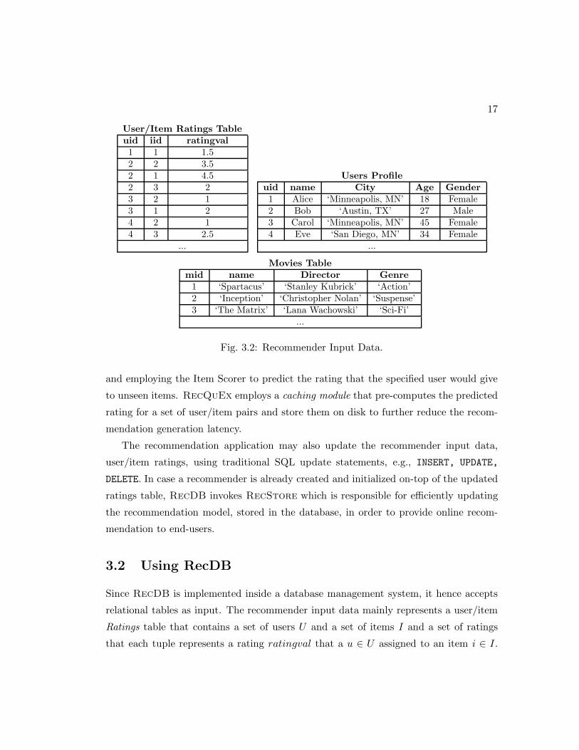
Fig. 3.2: Recommender Input Data.

and employing the Item Scorer to predict the rating that the specified user would give

to unseen items. RecQuEx employs a caching module that pre-computes the predicted

rating for a set of user/item pairs and store them on disk to further reduce the recom-

mendation generation latency.

The recommendation application may also update the recommender input data,

user/item ratings, using traditional SQL update statements, e.g., INSERT, UPDATE,

DELETE. In case a recommender is already created and initialized on-top of the updated

ratings table, RecDB invokes RecStore which is responsible for efficiently updating

the recommendation model, stored in the database, in order to provide online recom-

mendation to end-users.

3.2 Using RecDB

Since RecDB is implemented inside a database management system, it hence accepts

relational tables as input. The recommender input data mainly represents a user/item

Ratings table that contains a set of users U and a set of items I and a set of ratings

that each tuple represents a rating ratingval that a u ∈ U assigned to an item i ∈ I.

18

Ratings represent users expressing their opinions over items. Opinions can be a numeric

rating (e.g., one to five stars), or unary (e.g., Facebook “check-ins”). Also, ratings may

represent purchasing behavior (e.g., Amazon). Figure 3.2 gives an example of movie

recommendation data.

RecDB provides a tool to the system users to freely decide which attributes and

recommendation algorithm to be used in building a recommender. To this end, the

system allows its users to use a SQL-like clause to declare a new recommender by

specifying the recommender input data source and recommendation algorithm. This

section focuses on how users interact with the system. In particular, Section 6.1.1

explains the SQL clause for creating a new recommender, while Section 6.1.2 explains

the SQL for querying a certain recommender. Internals of RecDB that enable such

interface, i.e., indexing, maintenance, query processing and optimization, are described

in later sections.

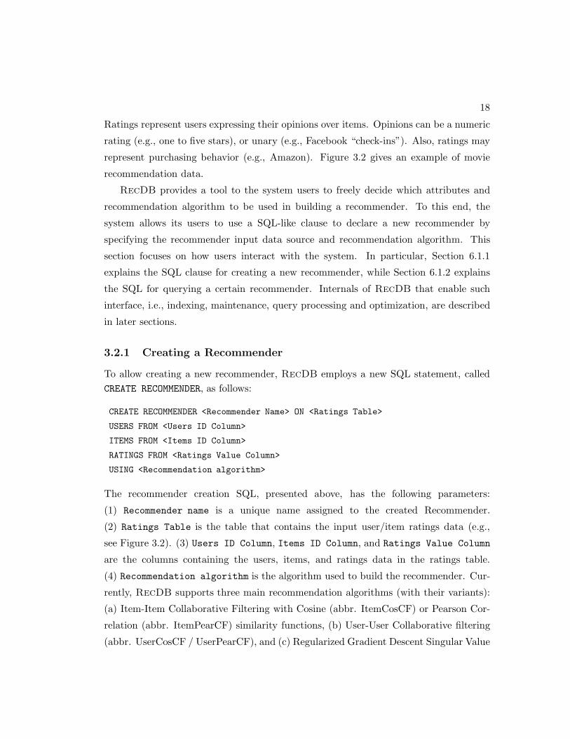
3.2.1 Creating a Recommender

To allow creating a new recommender, RecDB employs a new SQL statement, called

CREATE RECOMMENDER, as follows:

CREATE RECOMMENDER <Recommender Name> ON <Ratings Table>

USERS FROM <Users ID Column>

ITEMS FROM <Items ID Column>

RATINGS FROM <Ratings Value Column>

USING <Recommendation algorithm>

The recommender creation SQL, presented above, has the following parameters:

(1) Recommender name is a unique name assigned to the created Recommender.

(2) Ratings Table is the table that contains the input user/item ratings data (e.g.,

see Figure 3.2). (3) Users ID Column, Items ID Column, and Ratings Value Column

are the columns containing the users, items, and ratings data in the ratings table.

(4) Recommendation algorithm is the algorithm used to build the recommender. Cur-

rently, RecDB supports three main recommendation algorithms (with their variants):

(a) Item-Item Collaborative Filtering with Cosine (abbr. ItemCosCF) or Pearson Cor-

relation (abbr. ItemPearCF) similarity functions, (b) User-User Collaborative filtering

(abbr. UserCosCF / UserPearCF), and (c) Regularized Gradient Descent Singular Value

19

(c) User-Items Vector Table

UserID uVector

Alice {〈‘Spartacus’,1.5〉}Bob {〈‘Inception’,3.5〉;〈‘Spartacus’,4.5〉;〈‘The Matrix’,2〉}Carol {〈‘Inception’,1〉;〈‘Spartacus’,2〉}Eve {〈‘Inception’,1〉;〈‘The Matrix’,2.5〉}

(d) Item-Users Vector Table

Item iVector

‘Spartacus’ {〈Alice,1.5〉;〈Bob,4.5〉;〈Carol,1〉}‘Inception’ {〈Bob,3.5〉;〈Carol,1〉;〈Eve,1〉}‘The Matrix’ {〈Bob,2〉;〈Eve,2.5〉}

Fig. 3.3: Rating Table Storage Representation

Decomposition (abbr. SVD). If no recommendation algorithm is specified, RecDB em-

ploys by default the ItemCosCF algorithm.

Recommender Initialization. The initialization process consists of two steps:

(I) User/Item Rating Re-Arrangement: RecDB first re-arranges the user/item rating

matrix data on disk and stores it into the vector representation format. That format

represents the user/item ratings matrix as a table, namely the User Vector Table. The

user vector table consists of two columns: UserID: a unique user identifier and uVector:

a set of Key-Value pairs 〈iid, rating〉 that contains evert item iid rated by the user and

the respective rating value. The user vector table is indexed by a primary key index

created on the UserID field. Figure 5.1 gives the User Vector Table for the ratings

matrix given in Figure 3.2. To efficiently access item vectors instead of user vectors, we

also store the user/item ratings matrix transpose, called Item Vector Table, that also

consists of two columns: ItemID and iVector (see Figure 5.1).

(II) Model Building: In this step, RecDB employs a set of user defined functions

that train a recommendation model RecModel using the input data. The format of

the model depends on the underlying recommendation algorithm. For example, a rec-

ommendation model for the item-item collaborative filtering (cosine similarity measure)

model (ItemCosCF) [6] represents a similarity list of the tuples 〈ip, iq, SimScore〉, where

SimScore is the similarity between items ip and iq.

20

3.2.2 Updating a Recommender

To get the most accurate result, RecModel should be updated with newly inserted rating

by a user u assigned to an item i. However, doing so is infeasible as collaborative

recommendation algorithms employ complex computational techniques that are very

costly to update. The update maintenance procedure differs based on the underlying

recommender algorithm, specified in the CREATE RECOMMENDER statement. Yet, most of

the algorithms may call for a complete model rebuilding to incorporate any new update.

To avoid such prohibitive cost, we decide to update the RecModel only if the number

of new updates reaches to a certain percentage ratio N% (a system parameter) from

the number of entries used to build the current model. We do so because an appealing

quality of most supported recommendation algorithms is that as RecModel matures

(i.e., more data is used to build it), more updates are needed to significantly change the

recommendations produced from it.

3.2.3 Querying a Recommender

Once a recommender is created and initialized using the CREATE RECOMMENDER state-

ment, users can issue SQL queries that harnesses the created recommender to produce

recommendation to end-users, as follows:

SELECT <Select Clause>

FROM <Rating Table>

RECOMMEND <ItemID> TO <UserID> ON <RatingVal>

USING <Recommendation Algorithm>

WHERE <Where Clause>

Query Syntax. The SELECT and WHERE clauses are typical as in any SQL query.

The FROM clause may directly accept a [Ratings] table with the same schema passed to

the CREATE RECOMMENDER statement. The RECOMMEND clause is responsible for predicting

how much the system users would like the unseen items. The application developer also

needs to specify the ItemID (i.e., <ItemID>), UserID (i.e., TO <UserID>), and Rating

Value (i.e., ON <RatingVal>) Columns.

Query Semantics. The RECOMMEND clause returns a set of tuples S such that each

tuple s ∈ S; s =〈uid, iid, ratingval〉 represents a predicted rating score (ratingval) that

21

a user (uid) would give to an unseen item (iid) based on the recommendation algorithm

specified in the USING clause.

3.3 Case Studies

This section presents two case studies that manifest the usability of RecDB . Sec-

tion 3.3.1 presents a movie recommendation application that delivers movie recommen-

dation to end-users based on historical preferences. Section 3.3.2 highlights a Point-

of-Interest (POI) recommendation application that recommends Point-of-Interests to

end-users based on their spatial location.

3.3.1 Movie Recommendation

This section show how RecDB is used to build a movie recommendation application.

The data set leveraged by this application consists of three tables: (1) Users (uid,

name, age, city, gender): contains information about all users. Each user tuple

consists of a user ID, user name, age, home city, and gender. (2) Movies (mid, name,

director, genre): the set of movies saved in the database; each movie has a unique

ID, name, director, and genre. (3) Ratings (uid, mid, rating): The history of user

ratings such that each rating represents how much a user liked a movie she/he watched.

Creating a Movie Recommender

To create Recommender 3 (given below), the system user leverages the CREATE

RECOMMENDER SQL statement to declare MovieRec, a recommender that is created on

top of the Users, Movies, and Ratings database tables. We specify the item-item col-

laborative filtering method to be applied to the declared recommender.

Recommender 1 MovieRec: a ItemCosCF recommender created on the input data

stored in the Ratings table of Figure 3.2.

Create Recommender MovieRec On Ratings

Users From uid Item From iid Ratings From ratingval Using ItemCosCF

22

This SQL creates a recommender, named MovieRec inside RecDB . Rec is a traditional

recommender that can be queried to recommend a set of movies for a certain user, e.g.,

recommend me five movies.

Movie Recommendation Generation

An example of a movie recommendation query is given below:

Query 1 Return ten movies to user with ID 1 using the Item-Item Collaborative Fil-

tering algorithm.

Select R.uid, R.iid, R.ratingval

From Ratings as R

Recommend R.iid To R.uid On R.ratingVal Using ItemCosCF

Where R.uid=1 Order By R.ratingVal Desc Limit 10

In this case, RecDB uses the MovieRec recommender, which was created before using a

CREATE RECOMMENDER. Since this recommender was created based on the age attribute,

Query 11 will predict the ratings based on the algorithm passed to ItemCosCF algorithm.

The query finally returns the Top-10 movies to user 1 in a descending order of the

predicted rating value (ratingval).

3.3.2 Point-of-Interest (POI) Recommendation

Recently, applications like Yelp and Google maps have provided tools for end-users to

express their opinions over visited items, e.g., restaurants. That motivated the use of

recommender systems to suggest Point-Of-Interests (POIs) to end-users in urban areas.

In this section, we present a use case that serves as an anecdotal evidence to prove the

usefulness of RecDB . Consider the following scenarios:

Scenario 1 Alice plans to visit ‘Minneapolis’ for business. She looks for Hotel recom-

mendation in the ‘Minneapolis’ urban area.

In Scenario 1, the system first needs to retrieve hotels that lie within the ‘Minneapo-

lis’ area. Therefore, it predicts the rating that Alice would give to such hotels based on

23

the opinions of other users similar to her. In Scenario 2 (below), the system calculates

the distance between Alice’s current location and all restaurants. It also predicts a rat-

ing for each restaurant based on its similarity to restaurants already seen by Alice. The

system finally ranks restaurants based on both the spatial proximity score and predicted

rating score.

Scenario 2 Alice arrived to ‘Minneapolis’. She looks for nearby (personalized) restau-

rant recommendation.

In order to support POI recommendation, we integrate RecDB with PostGIS [46].

PostGIS is an extension to PostgreSQL that provides a SQL interface for users to

express spatial operations on geographical data. That way, users can spatially filter the

recommended POIs to only return those POIs that resides in a specified urban area.

That also allows users to rank POIs based on both its personalized recommendation

score and spatial proximity to the querying user.

Creating POI Recommenders

The following SQL creates a recommender, named POI-ItemCosCF-Rec, on the input

data stored in the HotelRatings table. POI-ItemCosCF-Rec can be accessed to predict

a rating that users would give to POIs based on the ItemCosCF algorithm.

Recommender 2 POI-ItemCosCF-Rec: an SVD recommender created on the Hotel-

Ratings table.

Create Recommender POI-ItemCosCF-Rec On HotelRatings

Users From uid Item From iid Ratings From ratingval Using ItemCosCF

The following SQL creates another recommender, named POI-SVD-Rec, on the the

RestaurantRatings table. POI-SVD-Rec can be accessed later to predict how much users

would like POIs based on the SVD recommendation algorithm.

Recommender 3 POI-SVD-Rec: a UserPearCF recommender created on the Restau-

rantRatings table.

24

Create Recommender POI-SVD-Rec On RestRatings

Users From uid Item From iid Ratings From ratingval Using SVD

Generating POI Recommendation

After initializing the POI recommenders, users may issue location-aware recommenda-

tion queries. For instance, to produce POI recommendation as given in Scenario 1, users

may issue the following SQL queries:

Query 2 Predict the rating that user 1 would give to Hotels that exist in the ‘Min-

neapolis’ urban area.

Select H.name, R.ratingval

From HotelRatings as R, Hotels as H, City as C


Where R.uid=1 AND R.iid=H.vid AND C.name = ‘Minneapolis’ AND

ST Contains(C.geom, H.geom)

In this case, RecDB uses the POI-ItemCosCF-Rec recommender, which was created

before using a CREATE RECOMMENDER. Query 2 predicts the ratings that user 1 would

give to unseen hotels using the RECOMMEND operator. However, the query leverages the

ST Contains() function (provided by PostGIS) to predict a rating only for those hotels

that lie within the extent of the ‘Minneapolis’ urban area.

Query 3 Recommend top-10 restaurants to user 1 that lies within a 500 meters distance

of her current location based on the UserPearCF algorithm.

Select V.name, V.address

From Ratings as R, Restaurants as V

Recommend R.iid To R.uid On R.ratingVal Using SVD

Where R.uid=1 AND R.iid=V.vid AND ST DWithin(ULoc, V.geom, 500)

Order By R.ratingVal Desc Limit 10

25

Query 3 harnesses the POI-SVD-Rec recommender, created earlier and initialized in-

side RecDB , to predict the ratings that user 1 would give to restaurants that lie within

500 meters range from the user current spatial location. To this end, Query 3 invokes the

ST DWithin() geometry function to filter out restaurants that are not spatially within

500 meters from the user location.

Query 4 Recommend top-10 restaurants that are close to user 1 current location based

on the SVD algorithm.

Select V.name, V.address

From Ratings as R, Restaurants as V

Recommend R.iid To R.uid On R.ratingVal Using SVD

Where R.uid=1 AND R.iid=V.vid

Order By CScore(R.ratingVal, ST Distance(V.geom, ULoc)) Desc Limit 3

Query 4 combines both the predicted rating score calculated using the UserPearCF

algorithm and the spatial proximity score using the PostGIS ST Distance() function.

The query finally returns the Top-3 restaurants.

Chapter 4

Online Recommendation Model

Maintenance

To get fresh (most accurate) recommendation, the recommendation model should be

updated with newly inserted user, item, or ratings data. A straightforward approach

is to use DBMS views to support online model management. This approach has major

drawbacks. (1) Inflexibility in supporting model truncation rules. For example, views

lack support for efficiently maintaining the top-k related objects for each object (user or

item) in the database. Furthermore, are incapable of understanding flexible truncation

rules [47] (e.g., maintain the top-k related objects for the 100 most popular objects in

the database, and only the top-m related objects otherwise, k > m). Such rules are

beneficial to the quality of recommendation [6, 17, 22]. (2) Inefficiency. Using a regular

view will incur serious query processing overhead. Essentially, this approach re-executes

the expensive model-building step for every recommendation generation query. On the

other hand, materialized views suffer from an update efficiency perspective. Depending

on the view definition, a materialized view may require a complete refresh upon receiving

an update to the base Rating table (e.g., complete refresh conditions in Oracle [48]).

Furthermore, we cannot specify how and when updates to the view occur in order to

tune update efficiency, e.g., update similarity scores only when the average item rating

moves outside a threshold. As we will see, such update rules are necessary in providing

efficient update support for some recommender models.

26

27

In this Chapter, we address the problem of providing online recommender model

maintenance for DBMS-based recommender systems. We present RecStore , a

RecDB module built inside the storage engine of a database system. RecStore en-

ables online model support for DBMS-based recommender systems (e.g., [38]) through

efficient incremental updates to only parts of the model affected by a rating update.

Thus, updating the recommender model does not involve significant overhead, nor re-

generation of the model from scratch. RecStore exposes the model to the query

processor as a standard relational table, meaning that existing recommender queries

can remain unchanged.

The basic idea behind RecStore is to separate the logical and internal representa-

tions of the recommender model. RecStore receives updates to the user/item rating

data (i.e., the base data for a collaborative filtering models) and maintains its internal

representation based on these updates. As RecStore is built into the DBMS storage

engine, it outputs tuples to the query processor though access methods that transform

data from the internal representation into the logical representation expected by the

query processor.

RecStore is designed with extensibility in mind. RecStore ’s architecture is

generic, and thus the logic for a number of different recommendation algorithms can

easily be “plugged into” theRecStore framework, making it a one-stop solution to sup-

port a number of popular recommender models within the DBMS. We provide a generic

definition syntax for RecStore , and provide implementation case studies for vari-

ous neighborhood-based [6, 42] collaborative filtering algorithms (e.g., item-based [21]

and user-based [19]). We also discuss support for other non-trivial recommendation

algorithms (e.g., [42, 49]).

RecStore is also adaptive to system workloads, tunable to realize a trade-off that

makes query processing more efficient at the cost of update overhead, and vice versa.

At one extreme, RecStore has lowest query latency by making update costs more

expensive; appropriate for query-intense workloads. At the other extreme, RecStore

minimizes update costs by pushing computation into query processing; appropriate for

update-intense workloads. For particularly update-intense workloads, RecStore also

performs load-shedding to process only important updates that significantly alter the

recommender model and change the answers to recommender queries.

28

RecStore requires a small code footprint, which is advantageous to implementa-

tion in existing database engines. Our prototype of RecStore , built inside Post-

greSQL [40], between the storage engine and query processor, requires approximately

600 lines of either modified or new code. Rigorous experimental study of our Rec-

Store prototype using a real workload from the popular MovieLens [50] recommender

system shows that RecStore exhibits desirable performance in both updates and query

processing compared to existing DBMS approaches that support online recommender

models using regular and materialized views.

The rest of this Chapter is organized as follows: Section 4.1 introduces the Rec-

Store architecture. Section 4.2 describes the functionality of RecStore . Finally,

Section 5.4 provides an experimental evaluation of RecStore .

4.1 RecStore Architecture

Figure 4.1 depicts the high-level architecture of RecStore , built inside the storage

engine of a DBMS. RecStore consists of the following main components:

• Intermediate store and filter. The intermediate store contains a set of statis-

tics, functions, and/or data structures that are efficient to update, and can be

used to quickly generate part of the recommender model. The data maintained

in the intermediate store is specific to the recommendation algorithm. Whenever

RecStore receives ratings updates (i.e., insertions, deletions, or changes to the

ratings table), it applies an intermediate filter that determines whether the update

will affect the contents of the intermediate store (Section 4.2.1).

• Model store and filter. The model store represents the materialized model

that matches the exact storage schema needed by the recommender algorithm

(e.g., (itm, rel itm, sim) for the item-based model covered in Section 2.1). Any

changes to the intermediate store goes through a model filter that determines

whether it affects the contents of the model store (Section 4.2.1).

29

Query

Processor

Storage Engine

DBMS

Index

Recommendation

Queries

Rating

Data

Intermediate

Filter

Intermediate Store

Model

Filter

Model Store

Scan

Rating

Updates

Access Methods RecStore

Fig. 4.1: RecStore Architecture

4.2 RecStore: Built-In Online DBMS-Based Recom-

menders

The main objective of RecStore is to bring online model support to existing recom-

mender queries for various workloads and recommendation algorithms. This objective

presents three main challenges that we address in the rest of this Chapter: (1) Efficient

online incremental maintenance of the recommender model, i.e., avoiding expensive

model regeneration with each update (Section 4.2.1). (2) The ability to adapt the

system to various workloads, e.g., query or update-intensive workloads (Section 4.2.2).

(3) The ability to support various existing recommender algorithms (Section 4.3).

4.2.1 Online Model Maintenance

This section describes the framework for online model maintenance within RecStore

. The framework is extensible, and its specific functionality is determined by the un-

derlying recommendation algorithm. While this approach may seem overly-tailored to

each specific algorithm, we note that many algorithms, especially collaborative filter-

ing, share commonalities in model structure. We defer such discussion until later in

Section 4.3. For now, we use the example of the item-based cosine model to illustrate

RecStore ’s approach to providing online model maintenance, consisting of two steps.

30

Step 1: Intermediate Filter

We describe the functionality of the intermediate filter with an example using the item-

based cosine algorithm described in Section 2.1. For this algorithm, the intermediate

store contains a “deconstructed” cosine score (Equation 2.4), where we store for each

item pair (ip,iq) that share at least one co-rated dimension (1) pdot(ip, iq), their partial

dot product, (2) lenp(ip, iq) and lenq(iq, ip), the partial length of each vector for only

the co-rated dimensions, and (3) co(ip, iq), the number of users who have co-rated items

ip and iq. This data is stored as a six-column relation, where the first two columns store

the item id pairs, while the last four columns store the four statistics just described.

RecStore employs an intermediate filter upon receiving a rating update R. The

intermediate filter performs three tasks in the following order. (1) Filter. This task

determines whether R will be used to update entries in the intermediate store. If not,

R is immediately dropped (but still stored in the ratings data). This step is required by

the adaptive maintenance and load shedding techniques discussed later Section 4.2.2.

In the general case this step will not drop any updates. (2) Enumeration. This task

determines all intermediate store entries E that will change due to R. For our item-

based cosine example with a new rating for item ip, E would contain all entries (ip,iq)

for which items ip and iq are co-rated by the user u. (3) Updates. Finally, all statistics,

functions, or data structures in the intermediate store associated with an entry e ∈ E

are updated. These updates are then forwarded to the model filter. For our item-based

cosine example, the stored statistics are updated as follows, assuming a new rating for

item ip with value sp: pdot(ip, iq) = pdot(ip, iq) + sp × sq, lenp(ip, iq) = lenp(ip, iq) + sp,

lenq(iq, ip) = lenq(iq, ip) + sq, and co(ip, iq) = co(ip, iq) + 1.

Together, the intermediate filter and store are the keys to efficient online model

maintenance in RecStore . The filter reduces update processing overhead by allowing

RecStore to only process the updates necessary to maintain an accurate intermediate

representation. The contents of the intermediate store keep computational overhead

low for online maintenance by allowing RecStore to quickly update the intermedi-

ate store and, once updated, quickly derive a final model score from the intermediate

representation.

31

Step 2: Model Filter

Upon receiving updates from the intermediate filter, the model filter executes the same

three tasks as the intermediate filter (i.e., filter, enumeration, and updates), except

applied to the model store instead of the intermediate store. Continuing our item-based

cosine example, its model store contains entries of the form (ip,iq,sim(ip,iq)), i.e., the

item-based model schema discussed in Section 2.1. The model filter uses the statistical

updates from the intermediate store for item pairs (ip,iq) to update the similarity score

in the model store entry (ip,iq, sim(ip,iq)) as follows per Equation 2.2: (1) If statistic

co(ip, iq) < 50, then sim(ip, iq) is updated as:

sim(ip, iq) =co(ip, iq) ∗ pdot(ip, iq)

50 ∗√

lenp(ip, iq)√

lenq(ip, iq)

(2) If statistic co(ip, iq) ≥ 50, we update sim(ip, iq) as:

sim(ip, iq) =pdot(ip, iq)

√

lenp(ip, iq)√

lenq(ip, iq)

Updating the similarity score is the final step in the RecStore online maintenance

process.

4.2.2 Adaptive Strategies for System Workloads

This section discusses how RecStore adapts to different workload characteristics. We

first discuss generic maintenance strategies that help realize an update and query effi-

ciency trade-off. We then discuss load-shedding for update-intensive workloads.

Update vs. Query Efficiency Trade-off

While the intermediate and model store are beneficial to RecStore , their sizes may

lead to non-trivial maintenance costs. For instance, in item-item or user-user collabo-

rative filtering, the size of the model can reach O(n2), where n is the number of items

(or users). In this case, RecStore could be responsible for updating and maintaining

data for O(n2) items (or users) in its intermediate and model store, leading to burden-

some maintenance costs. In this section, we explore a trade-off: reducing the storage

and maintenance of data in the intermediate store and model store (i.e., the internal

maintenance approach) in return for sacrificing query processing (i.e., recommendation

generation) efficiency.

32

RecStore can be tuned to realize an efficiency trade-off between updates and query

processing. The basic idea is to maintain α entries in the intermediate store, β entries in

the model store, and require the invariant that α ≥ β, i.e., all entries in the model store

are also maintained in the intermediate strore. Both values cannot be greater thanM:

the total possible number of entries, a model-specific value (e.g., for item-based models

M = I2).

Low values of α and β imply low incremental update latency as the filters udpate

fewer entries in the intermediate and model stores. On the other hand, during query

processing, the access algorithms must service requests from the query processor by

producing model values in the following order of efficiency: (1) directly from the model

store if the entry is maintained there. (2) If the entry is not maintained in the model store

but maintained in the intermediate store, the model value is produced on-demand from

the intermediate store (e.g., from the intermediate statistics covered in Section 4.2.1 for

the item-based cosine algorithm). (3) If the entry is not maintained in the intermediate

nor the model store, the model value must be produced on-demand using the base

ratings data (e.g., using Equation 2.1 for the item-based cosine algorithm). Thus, as

α and β decrease, query processing latency increases as more model values must be

produced on demand. Larger values of α and β have a reverse effect on update and

query processing efficiency.

Using the maintenance parameters α and β allows RecStore to be tuned for a

wide range of workloads. More update-intense workloads can lower values of α and β at

the cost of increasing recommender query latency. Meanwhile, query-intense workloads

can use larger values of α and β at the cost of increasing update overhead. We now

explore several strategies for α and β settings; experimental analysis for these strategies

is given in Section 5.4.

• Extreme Approaches. Two extreme approaches can be taken by RecStore

: (1) Materialize all . In this approach α = β = M, meaning RecStore ’s

intermediate and model stores maintain all required model information. RecStore

filters just apply the conditions imposed by the specific similarity functions upon

receiving a rating update. Recommendation generation, i.e., the query processing

functionality that generates recommended items, is most efficient at this extreme.

However, storage and maintenance costs are at their highest with this approach.

33

(2) Materialize none. In this approach α = β = 0, and basically mimics the

use of regular DBMS views that we recompute model values on demand. In this

approach there is no need for the intermediate store, model store, nor filters.

Recommendation generation for this approach is very expensive, but incurs no

storage and maintenance costs as nothing is maintained.

• Intermediate Store Only. In this approach α = M and β = 0. This ap-

proach (abbr. Intermediate Only) represents a middle ground between Material-

ize All and Materialize None, where we materialize the intermediate store in full

for all required model information, while not maintaining the model store. This

means that the initial filter will be applied on all incoming updates as described

in Section 4.2.1, while there is no filter for the model store. The recommendation

generation process for a requested object o (e.g., item or user) needs to rebuild

part of the model store that includes o using the fully maintained intermediate

store. This rebuilding process makes this approach incur higher query processing

cost compared to the Materialize All approach, but much lower query processing

cost than the Materialize None approach. On the other hand, storage and main-

tenance costs are lower than the materialize all approach, as the model store is

nonexistent.

• Full Intermediate Store and Partial Model Store. This approach (abbr.

Partial Model) sets α =M and β = N , and represents a middle ground between

the Materialize all and Intermediate Only approaches. This approach materializes

only a portion of the model store, i.e., only N objects (e.g., items or users),

while materializing the intermediate store in full. We employ hotspot detection

(described in Section 4.2.2) to select theN items in the model store. This approach

directs the initial filter will be applied to all incoming updates. All updates made

to the intermediate store are still forwarded to the model filter as described in

Section 4.2.1, however, the model filter only accepts updates for the qualifying N

objects, and their their related objects, that are maintained in the model store.

The query processing and storage/maintenance overhead for this approach lies

between the Materialize all and Intermediate Only approaches.

• Partial Intermediate Store and Partial Model Store. This approach sets

34

α = K and β = N , and is similar to the Partial Model approach, except that we

also partially materialize the intermediate store. The model store still maintains

data for N objects, while the intermediate store maintains data for K objects.

These K and N objects are derived using hotspot detection (described next in

Section 4.2.2). This approach directs the initial filter only accepts incoming up-

dates for the K objects (items of users), and their their related objects, that

qualify for storage in the intermediate store. The model filter remains unchanged

from the Partial Model approach. The query processing and storage/maintenance

overhead for this approach lies between the Partial Model and Intermediate Only

approaches.

HotSpot Detection

For the approaches that use partial materialization, α and β should ideally be set to

ensure the maintenance of model hotspots, i.e., popular or frequently accessed entries.

This setting assures efficient query processing over popular model entries, while sacrific-

ing higher query latency for less popular model entries. We use two methods to detect

hotspots. (1) Most accessed. Keep the α and β most accessed entries from the model

determined by simple usage statistics from the access methods. (2) Most rated. Keep

the α and β most popular entries in the model determined by association with the most

ratings (e.g., most-rated movies, users who rate the most movies).

Load Shedding

For the special case of update-intense workloads where the system is incapable of pro-

cessing all ratings updates, RecStore is capable of load-shedding. The goal of load-

shedding is to process only updates that significantly alter the recommender model, thus

changing the answer to recommender queries. Load-shedding techniques are model-

specific, and RecStore executes these techniques in a special filter before the interme-

diate filter.

As an example, consider the item-based cosine method, where an update should

only be processed if it changes the order in the model similarity lists. In this case,

altered order in any similarity list can potentially change the answer to a recommender

query per Equation 2.4. An effective heuristic approach to achieve this goal is to process

35

DEFINE RECSTORE MODEL ItmItmCosine

FROM Ratings R1, Ratings R2

WHERE R1.itemId <> R2.ItemId AND R1.userId = R2.userId

WITH INTERMEDIATE STORE:

(R1.itemId as item, R2.itemId as rel_itm, vector_lenp,

vector_lenq, dot_prod, co_rate)

WITH INTERMEDIATE FILTER:

ALLOW UPDATE WITH My_IntFilterLogic(),

UPDATE vector_lengthp AS R1.rating*R1.rating,

UPDATE vector_lengthq AS R2.rating*R2.rating,

UPDATE dot_prod AS R1.rating*R2.rating,

UPDATE co_rate AS 1

WITH MODEL STORE:

(R1.itemId as item, R2.itemId as rel_itm, COMPUTED sim)

WITH MODEL FILTER:

ALLOW UPDATE WITH My_ModFilterLogic(),

UPDATE sim AS

if (co_rate < 50)

co_rate*dot_prod/50*sqrt(vector_len1)* sqrt(vector_len2);

else

co_rate/sqrt(vector_len1)* sqrt(vector_len2);

Fig. 4.2: Registering a recommendation algorithm

updates that change intermediate store entries with a co-rating count (i.e., the statistic

co(ip, iq)) below a pre-set threshold T . The intuition here is that low co-rated items

have less terms defining their cosine distance, thus an update will likely alter the score

significantly compared to more highly co-rated items. Of course, more sophisticated

statistical techniques can apply. However, any load-shedding approach should remain

simple to evaluate and maintain due to its mission-critical purpose.

4.3 RecStore Extensibility

RecStore provides a generic extensible architecture capable of supporting different

recommendation algorithms. This section first demonstrates how to register a recom-

mendation algorithm with RecStore . We then provide various case studies demon-

strating how RecStore accommodates other item-based collaborative filtering meth-

ods. Finally, we discuss how RecStore supports recommendation algorithms beyond

“neighborhood-based” collaborative filtering.

36

4.3.1 Registering a Recommender algorithm

We provide a syntax for registering a new recommender algorithm model within Rec-

Store . Figure 4.2 gives an example for registering the item-based cosine algorithm.

Registration begins by first defining the model name, and then providing a from and

optional where clause to specify the base data used in the model. For the item-based

cosine model, the base data comes from the Ratings relation, and the where-clause de-

fines a relational constraint (in the form of a self-join) declaring that model entries are

(non-equal) items that are co-rated by the same user. The major clauses are:

• WITH INTERMEDIATE STORE: defines the data in the intermediate

store; in this case the intermediate statistics for the item-based cosine algorithm.

• WITH INTERMEDIATE FILTER: defines the intermediate filter in two

parts. (1) Allow Updates With defines the logic for filtering incoming updates

(task 1 discussed in Section 4.2.1), currently contained in a user-defined function.

(2) Update defines how to compute data in the intermediate store when given a

rating update that is not filtered ; the logic can be given directly or contained in a

user-defined function.

• WITH MODEL STORE: defines the name and schema of the model store,

this schema is exposed to the rest of the DBMS and used by the recommender

queries. Any attributes computed from data in the intermediate store are given the

COMPUTED prefix. Our example item-based cosine follows the schema discussed

in Section 4.2.1, where the value sim is a computed attribute.

• WITH MODEL FILTER: follows the same syntax as the intermediate filter,

with the exception that the compute clause defines how to update the model store

values using data from the intermediate store.

4.3.2 Item-Based Collaborative Filtering

We now discuss RecStore registration for two other item-based collaborative filter-

ing algorithms [21], namely probabilistic and Pearson item-based recommenders. We

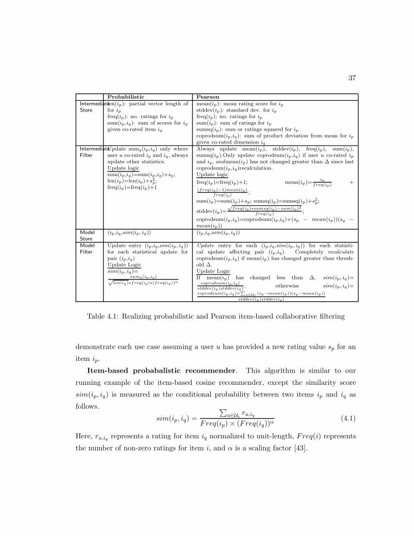
37

Probabilistic Pearson

Intermediate

Store

len(ip): partial vector length offor ipfreq(ip): no. ratings for ipsum(ip,iq): sum of scores for ipgiven co-rated item iq

mean(ip): mean rating score for ipstddev(ip): standard dev. for ipfreq(ip): no. ratings for ipsum(ip): sum of ratings for ipsumsq(ip): sum or ratings squared for ipcoprodsum(ip ,iq): sum of product deviation from mean for ipgiven co-rated dimension iq

Intermediate

Filter

Update sumq(ip,iq) only whereuser u co-rated ip and iq , alwaysupdate other statistics.Update logicsum(ip,iq)=sum(ip,iq)+sp;len(ip)=len(ip)+s2p;freq(ip)=freq(ip)+1

Always update mean(ip), stddev(ip), freq(ip), sum(ip),sumsq(ip).Only update coprodsum(ip ,iq) if user u co-rated ipand iq, andmean(ip) has not changed greater than ∆ since lastcoprodsum(ip ,iq)recalculation.Update logic

freq(ip)=freq(ip)+1; mean(ip)=sp

freq(ip)+

(freq(ip)−1)mean(ip)

freq(ip);

sum(ip)=sum(ip)+sp; sumsq(ip)=sumsq(ip)+s2p;

stddev(ip)=

√freq(ip)∗sumsq(ip)−sum(ip)2

freq(ip);

coprodsum(ip ,iq)=coprodsum(ip,iq)+(sp − mean(ip))(sq −mean(ip))

Model

Store

(ip,iq,sim(ip, iq)) (ip,iq,sim(ip, iq))

Model

Filter

Update entry (ip,iq,sim(ip, iq))for each statistical update forpair (ip,iq)Update Logicsim(ip, iq)=

sumq(ip,iq)√len(iq)∗freq(ip)∗(freq(iq))α

Update entry for each (ip,iq,sim(ip, iq)) for each statisti-cal update affecting pair (ip,iq). Completely recalculate

coprodsum(ip ,iq) if mean(ip) has changed greater than thresh-old ∆.Update LogicIf mean(ip) has changed less than ∆, sim(ip, iq)=

coprodsum(ip,iq)

stddev(ip)stddev(iq), otherwise sim(ip, iq)=

coprodsum(ip,iq)=∑

u∈Uc(sp−mean(ip))(sq−mean(ip))

stddev(ip)stddev(iq)

Table 4.1: Realizing probabilistic and Pearson item-based collaborative filtering

demonstrate each use case assuming a user u has provided a new rating value sp for an

item ip.

Item-based probabalistic recommender. This algorithm is similar to our

running example of the item-based cosine recommender, except the similarity score

sim(ip, iq) is measured as the conditional probability between two items ip and iq as

follows.

sim(ip, iq) =

∑

u∈Ucru,iq

Freq(ip)× (Freq(iq))α(4.1)

Here, ru,iq represents a rating for item iq normalized to unit-length, Freq(i) represents

the number of non-zero ratings for item i, and α is a scaling factor [43].

38

The second column of Table 4.1 provides an approach to implementing the item-

based probabilistic algorithm in RecStore . The intermediate store contains (1) the

partial vector length for item iq (len(iq)), (2) the total number of ratings for ip (freq(ip)),

and (3) the item-pair statistic maintains the running sum ratings for item ip given that

it is co-rated with an item iq (sum(ip,iq)). The intermediate filter updates all single-

item statistics, while only updating the pair statistic for which items ip and iq are both

rated by user u. Each statistic update requires constant time. The model filter, upon

receiving changes to the intermediate statistics, updates the similarity score sim(ip,iq)

for pairs ip,iq in constant time using the intermediate statistics (equation given in the

last row, second column of Table 4.1).

Item-based Pearson recommender. This algorithm is similar to the item-based

cosine algorithm, except it measures the similarity between objects using their Pearson

correlation coefficient as follows.

sim(ip, iq) =

∑

u∈Uc(Ru,ip −Rip)(Ru,iq −Riq )

σipσiq(4.2)

Uc represents users who co-rated items ip and iq, Ru,ip and Ru,iq represent a user’s

ratings, and Rip and Riq represent the average rating for items ip and iq, respectively.

σip and σiq are the standard deviations for ip and iq

The third column of Table 4.1 provides an approach to implementing the Pearson

algorithm in RecStore . The intermediate store maintains for an item ip its mean

rating value for an item (mean(ip)), its standard deviation of rating values (stddev(ip)),

the total number of ratings for ip (freq(ip)), the sum of ratings for ip (sum(ip)), and

the sum of the squared rating values for ip (sumsq(ip)). The intermediate store also

maintains coprodsum(ip ,iq): the sum of the product of deviations from the mean (i.e.,

the numerator in Equation 4.2) for an item pair (ip,iq) given that they share at least

one co-rated dimension. The intermediate filter updates all single-item statistics (those

maintained for ip only). The statistic coprodsum( ip,iq) is incremented by the product

of the deviation of user u’s score for ip (i.e., sp) from the newly calculated mean(ip),

and the deviation of iq (i.e., sq) from the stored mean for item iq (mean(iq)). Note that

previous rating scores for ip in the sum deviated from different means, since mean(ip)

changed with this update. In essence, we are willing to forgo this difference in accuracy

as long as mean(ip) has not changed by at least a value ∆ since the last calculation of

39

coprodsum(ip ,iq). What we gain in this trade-off is efficiency, since updating coprod-

sum(ip,iq) is more efficient than recalculating the sum from scratch.

The model filter updates the similarity score sim(ip,iq) for pairs ip,iq in the model

store using one of two algorithms (both given in the last row, third column of Table 4.1).

(1) If the value mean(ip) had not changed by ∆ since the last recalculation of coprod-

sum(ip,iq), then we can update sim(ip,iq) efficiently by dividing coprodsum(ip,iq) by

the product of the standard deviations. Otherwise, we must recalculate the value of

coprodsum(ip ,iq) from scratch for each entry using the current value of mean(ip).

4.3.3 User-based Collaborative Filtering

The model for user-based collaborative filtering [19] is similar to the item-based ap-

proach, except that the model stores groups of similar users (as described in Section 2.1).

Thus, the use cases previously discussed for the item-based approach can apply directly

to the user-based approach, with the exception that similarity is measured over user

vectors in the item rating space.

4.3.4 Non-“neighborhood-based” Collaborative Filtering within Rec-

Store

Many other recommendation algorithms use models that are not similarity-based lists,

as is the case with the “neighborhood-based” collaborative filtering techniques we have

explored. In general, RecStore can support these different recommendation tech-

niques as long as their models can be represented by sufficient statistics to update the

model incrementally. For instance, recommendation algorithms that use sophisticated

probabilistic models (e.g., Bayesian Networks [42], Markov decision processes [51]) do

not lend themselves well to incremental updates, due to the computationally intense

optimization process used to learn their parameters. On the other hand, algorithms

that use linear regression to learn a rating prediction model [21] can fit easily within

RecStore . In this case, the intermediate store can maintain the general linear model

statistics: X (the regression design matrix), XT (X transposed) and f (the regressand).

It is known that these statistics are incrementally updatable and sufficient to learn un-

known regression coefficients by solving the system of equations [52]: XTXβ = XT f ,

40

where β represents the learned regression coefficients. The source for these statistics

depends on the recommendation algorithm. Examples include ratings vectors [21], a

multi-dimensional ratings base (e.g., multi-dimensional recommenders [35]), or item

attributes (e.g., content-based recommenders [53]).

4.4 Experimental Evaluation

This section experimentally evaluates the performance of a prototype of RecStore

implemented in between the storage engine and query processor of the PostgreSQL 8.4

database system [40] using the real-world Movielens 10M rating data set [50]. We test

various RecStore adaptive maintenance strategies based on α and β proposed in Sec-

tion 4.2.2: materialize all (abbr. matall) where α = β =M , intermediate only (ionly)

where α=M and β = 0 , partial model hotspot maintenance where α=M and β is set

to 20% of all movies (pm-m), and partial intermediate and model hotspot maintenance

(pm-mi) where α and β are set to 40% and 20% of all movies. We also compare against

regular (viewreg) and materialized DBMS views (viewmat). The viewreg approach

is implemented using a regular PostgreSQL view, but since PostgreSQL does not sup-

port materialized views, we provide a fair simulation of viewmat within RecStore

by maintaining a materialized Model store without the use of an intermediate store.

We provide experiments for: (1) Partial maintenance strategies (Section 4.4.1),

(2) update efficiency (Section 4.4.2), (3) query efficiency using the query given in Fig-

ure 2.6 (Section 4.4.3), and (4) a real recommender system workload trace consisting of

interleaved queries and updates (Section 4.4.4). Each experiment is run for both the co-

sine and probabilistic item-based recommendation algorithm (details of both algorithms

given in Section 4.3).

The experiment machine is an Intel Core2 8400 at 3Ghz with 4GB of RAM running

Ubuntu Linux 8.04. Our performance metric is the elapsed time over an average of five

runs reported by the PostgreSQL EXPLAIN ANALYZE command.

4.4.1 Hotspot Detection Strategies

This experiment studies the effectiveness of our two hotspot detection strategies covered

in Section 4.2.2: most-rated (abbr. rated) and most-accessed (abbr. accessed). We

41

0 5

10 15 20 25 30 35 40 45 50

pm-m

(cos)

pm-m

(prob)

pm-m

i(cos)

pm-m

i(prob)

Tim

e (

se

c)

rated accessed

(a) Query

0

1

2

3

4

5

6

pm-m

(cos)

pm-m

(prob)

pm-m

i(cos)

pm-m

i(prob)

Tim

e (

se

c)

rated accessed

(b) Update

Fig. 4.3: Hotspot Detection

0

2

4

6

500 2.5K 4.5K 7K

Tim

e (

sec)

Number of Updates

viewreg

viewmat

pm-mi

pm-m

ionly

matall

(a) Cosine

0

2

4

6

500 2.5K 4.5K 7K

Tim

e (

sec)

Number of Updates

viewreg

viewmat

pm-mi

pm-m

ionly

matall

(b) Update

Fig. 4.4: Update Efficiency

use a real workload trace consisting of the continuous arrival of both ratings updates

and recommender queries against the MovieLens system [9, 50]. We start with a Rat-

ings table that already contains 950K ratings, and report the total time necessary to

process 1K ratings updates interleaved with 40 recommendation generation queries for

different users. Figures 4.3(a) and 4.3(b) report performance for rated and accessed

using both the pm-mi and pm-m approaches implementing the cosine and probabilis-

tic algorithms. The update performance is relatively similar between the rated and

accessed strategies for all cases. However, the query performance of rated over ac-

cessed exhibits a 50% speedup, as rated is able to keep model data in the intermediate

and model store requested by the recommendation generation queries. Thus, in the rest

42

of this section, we employ the rated strategy for both pm-mi and pm-m .

4.4.2 Update Efficiency

This experiment studies update efficiency and scalability. We start with a Ratings table

already containing 950K rating tuples, and measure the total time it takes to process

500, 2.5K, 4.5K, and 7K updates, respectively. Figures 4.4(a) and 4.4(b) give the re-

sults for the cosine and probabilistic algorithms, respectively. For both algorithms, all

approaches exhibit the same relative performance. The materialized view (viewmat)

incurs the most overhead of all approaches. This performance is due to the need, on

every update, to recalculate the model score from scratch using the ratings data. The

RecStore matall strategy, on the other hand, incurs less update overhead compared

to viewmat due to its intermediate store, that helps it to efficiently update the model

store. This experiment confirms that RecStore overcomes the update efficiency draw-

back of materialized views. Both ionly and pm-mi exhibit better performance, with

ionly doing slightly better due to not having to maintain a partial model store. Both

matnone and pm-mi exhibit the best performance due to the low (or non-existent)

storage and maintenance costs.

4.4.3 Query Efficiency

This experiment studies query efficiency and scalability. We measure the time to per-

form the recommender query given in Figure 2.6 for a user X as the number of tuples

in the Ratings table increases from 5K to 70K. We choose user X as the user that has

rated the most movies. Figures 4.5(a) and 4.6(a) give the results for the cosine and

probabilistic recommendation algorithms, respectively. The viewreg approach (a regu-

lar DBMS view) performs very poorly, as it must calculate all requested model scores

from scratch from the ratings relation. The pm-mi approach exhibits performance

between matnone and the rest of the approaches, as it must service a fraction of its

requests from the ratings data, similar to viewreg . Figures 4.5(b) and 4.6(b) zoom in

on the matall , ionly , and pm-m approaches for the cosine and probabilistic models,

respectively. As expected, the matall approach exhibits the best query processing per-

formance as it must only retrieve values from the model store. Both ionly and pm-m

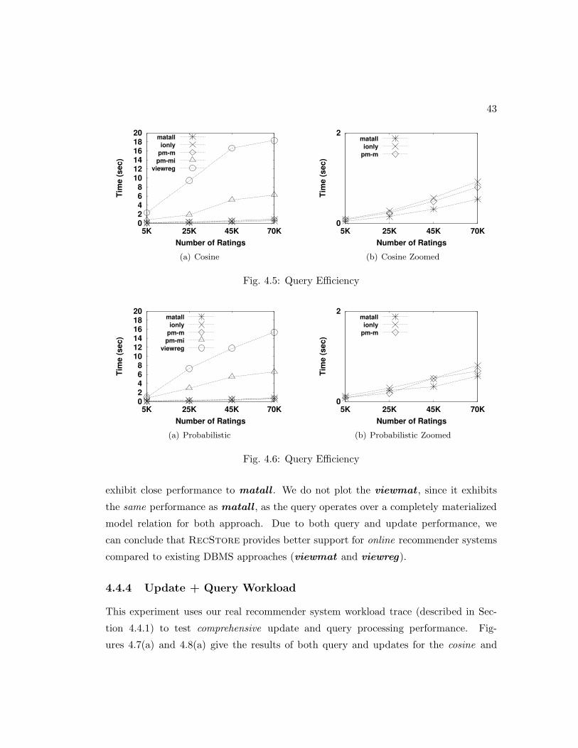
43

0 2 4 6 8

10 12 14 16 18 20

5K 25K 45K 70K

Tim

e (

sec)

Number of Ratings

matall

ionly

pm-m

pm-mi

viewreg

(a) Cosine

0

2

5K 25K 45K 70K

Tim

e (

sec)

Number of Ratings

matall

ionly

pm-m

(b) Cosine Zoomed

Fig. 4.5: Query Efficiency

0 2 4 6 8

10 12 14 16 18 20

5K 25K 45K 70K

Tim

e (

sec)

Number of Ratings

matall

ionly

pm-m

pm-mi

viewreg

(a) Probabilistic

0

2

5K 25K 45K 70K

Tim

e (

sec)

Number of Ratings

matall

ionly

pm-m

(b) Probabilistic Zoomed

Fig. 4.6: Query Efficiency

exhibit close performance to matall . We do not plot the viewmat , since it exhibits

the same performance as matall , as the query operates over a completely materialized

model relation for both approach. Due to both query and update performance, we

can conclude that RecStore provides better support for online recommender systems

compared to existing DBMS approaches (viewmat and viewreg).

4.4.4 Update + Query Workload

This experiment uses our real recommender system workload trace (described in Sec-

tion 4.4.1) to test comprehensive update and query processing performance. Fig-

ures 4.7(a) and 4.8(a) give the results of both query and updates for the cosine and

44

0 10 20 30 40 50 60 70 80 90

query updates

Tim

e (

sec)

matallviewmat

ionlypm-m

pm-miviewreg

(a) Cosine

0

1

2

3

4

5

6

7

query updates

Tim

e (

sec)

matallviewmat

ionlypm-m

(b) Cosine Zoomed

Fig. 4.7: Real Workload

0

10

20

30

40

50

60

70

query updates

Tim

e (

sec)

matallviewmat

ionlypm-m

pm-miviewreg

(a) Probabilistic

0

1

2

3

4

5

6

7

8

query updates

Tim

e (

sec)

matallviewmat

ionlypm-m

(b) Probabilistic Zoomed

Fig. 4.8: Real Workload

probabilistic algorithms, respectively. Both viewreg and pm-mi exhibit poor query

processing performance for the workload, with viewreg performing almost an order

magnitude worse than other approaches. While the viewreg performance is expected,

the pm-mi performance is more surprising. Both viewreg and pm-mi exhibit the best

update performance out of all approaches, as confirmed by our previous experiments

(Section 4.4.2). However, the query processing performance of viewreg makes it an

unattractive alternative, while the update/query processing tradeoff for pm-mi is a

borderline choice due to its high query processing penalty. Figures 4.7(b) and 4.8(b)

remove the viewreg and pm-mi numbers to zoom in on the other approaches for the co-

sine and probabilistic models, respectively. Both the matall and viewmat approaches

45

exhibit the same query processing performance that is superior to ionly and pm-m .

As for updates, we note again that matall (RecStore ) provides more efficient update

performance over viewmat (materialized views). Meanwhile, pm-m and ionly show

superior update performance to matall and viewmat , with ionly providing the best

performance.

In this experiment, we can observe the update/query processing trade-off discussed

in Section 4.2.2 for high values of α and β (matall) compared to lower values of α and

β (ionly and pm-mi). Thus, for slightly more update-heavy recommender systems,

the ionly or pm-mi is preferable due to efficient updates with little query processing

penalty. Meanwhile, for more query-heavy systems, the matall approach is preferable

with tolerable update penalty.

Chapter 5

Recommendation Query

Processing and Optimization

A main challenge is how to efficiently execute queries over an initialized recommender.

One solution is to implement a Stored Procedure that performs the recommendation

query functionality over the initialized recommender. However, this approach is very

limiting since it does not provide much flexibility for the database engine to optimize

incoming queries. This section discusses RecQuEx a RecDB module built inside

the database query execution engine for internal processing of recommender queries.

RecQuEx encapsulates the recommendation functionality into a new family of query

operators, termed Recommend. Being a query operator allows the recommendation

functionality to be a part of a larger query plan that includes other query operators,

e.g., selection, projection, and join. It also means that the recommendation functionality

will be treated as a first class citizen operation, allowing a myriad of query optimization

techniques that can be integrated to speed up recommendation queries.

To further reduce the recommendation application latency, RecQuEx pre-computes

the predicted rating scores and caches the corresponding {user,item,rating} entries

inside the database system. Storing and Maintaining the predicted rating for all

{user,item,rating} entries may preclude system scalability. Hence, RecQuEx adap-

tively decides, based on the query/update workload, which entries to maintain with

the main goal to reduce the overall recommender storage and maintenance overheard

46

47

(a) Item-Item Similarity Matrix

Item ItemNeighbors

‘Spartacus’ {〈‘Spartacus’,0.5〉;...}‘Inception’ {〈‘Spartacus’,0.5〉;〈‘The Matrix’,1〉;...}‘The Matrix’ {〈‘Inception’,1〉;〈‘Spartacus’,0.2〉;...}

(b) User-User Similarity Matrix

User UserNeighbors‘Alice’ {〈Bob,0.5〉;〈Carol,0.5〉;...}‘Bob’ {〈Alice,0.5〉;〈Eve,1〉;...}‘Carol’ {〈Alice,1〉;〈Eve,0.2〉;...}‘Eve’ {〈Bob,0.2〉;〈Carol,0.2〉;...}

Fig. 5.1: Item-Item (User-User) Collaborative Filtering Model

without compromising the recommendation generation performance.

Experiments, based on actual system implementation inside PostgreSQL, using

real data extracted from MovieLens [54] (Movie Recommendation Application) and

Foursquare [55] (Point-of-Interest Recommendation Application), show that RecQuEx

exhibits high performance for large-scale recommendation scenarios.

In summary, this chapter introduces the following: (1) RecQuEx – a unified ap-

proach for processing recommendation requests inside the database engine. (2) A family

of novel query operators, called Recommend, that realize the recommendation algo-

rithms inside the database query processor (Section 5.1). (3) Recommendation-aware

operators that further optimize the recommendation operation with other operators (se-

lection, join, and ranking) (Sections 5.3.1 and 5.3.2). (4) A materialization scheme that

caches the pre-computed predicted rating scores to further reduce the recommendation

latency (Section 5.3.3).

5.1 Recommendation Operators

RecQuEx employs three main versions of the Recommend operator; one for each

recommendation algorithm. Each operator take as input a ratings table and return a

set of tuples S such that each tuple s ∈ S; s =〈uid,iid,ratingval〉 represents a predicted

rating score ratingval for each item iid unseen by user uid. This section first describes

48

Algorithm 1 ItemCF-Recommend

1: /* load User Vector Table block by block in Memory */2: for each user u ∈ UserVector do3: UserItems ← List of User u rated items in ItemNeighborhood4: /* load Item Neighborhood Table block by block in Memory */5: for each item i ∈ ItemNeighborhood do6: ItemNeighbors ← List of item similar to item i in ItemNeighborhood7: if item i ∈ UserItems then8: ru,i ← Rating that u gave to i9: else

10: CandItems ← ItemNeighbors ∩ UserItems11: if CandItems not equal φ then12: ru,i ← Predict(u,i, UserItems, ItemNeighbors)13: else14: ru,i ← 015: EMIT 〈u, i, ru,i〉

the recommendation operators and then explains how they are integrated in the SQL

query pipeline.

5.1.1 Item-Item Collaborative Filtering Operator

RecQuEx stores the item-item similarity list as a table, called the Item Neighborhood

Table. This table consists of two columns: (1) ItemID: a unique item identifier and

(2) ItemNeighbors: a set of Key-Value pairs 〈iid,simscore〉 that contains every item iid

that belongs to ItemID neighborhood. The Item Neighborhood Table is indexed by a

primary key index created on the ItemID field. Figure 5.1(a) gives an example of the

Item Neighborhood Table. RecQuEx adopts the same storage layout for the user-user

collaborative filtering algorithm, but in this case stores the User Neighborhood table

instead of items (see Figure 5.1(b)).

For an incoming query, the query planner invokes the ItemCF-Recommend op-

erator when the USING clause specify the Item-Item Collaborative Filtering Algorithm

(i.e., ItemCosCF or ItemPearCF). Algorithm 1 gives the pseudocode of the ItemCF op-

erator. The ItemCF operator accesses both the user vector table (UserVector) and an

item neighborhood table (ItemNeighborhood). The operator then returns a set of tuples

S such that each tuple s ∈ S; s = 〈u, i, ru,i〉 represents a user u, item i (unseen by

49

user uid), and a rating ru,i. ItemCF fetches UserVector block by block to retrieve each

tuple 〈u; {(i1, ru,i1), ..., (im, ru,im)}〉. In a nested-loop fashion, the algorithm scans Item-

Neighborhood block by block and saves the currently retrieved block in an in-memory

buffer. If an item i is already rated by u, we set ru,i to the rating that u already assigned

to i. In case u did not rate i, we first determine whether the set of similar items to

i ItemNeighbors intersects the set of items rated by u (i.e., UserItems). If there in no

overlap, the algorithm sets ru,i to 0. Otherwise, ItemCF invokes Predict() to esti-

mate the rating value ru,i. Finally, ItemCF emits the tuple 〈u, i, ru,i〉 up in the query

pipeline. The Predict procedure takes as input the user u, item i, the items rated by u

UserItems, and the set of items similar to i ItemNeighbors. It then employs an aggregate

function to estimate how much user u would like item i and returns a predicted rating

accordingly. Example is given below:

Query 5 Predict the rating that users would give to unseen items based on the Item-

Based Collaborative Filtering Algorithm.

Select R.uid,R.iid, R.ratingval

From Ratings as R

Recommend R.iid To R.uid On R.ratingval Using ItemCosCF

By specifying the Recommend clause and the Ratings table in the From clause, Rec-

QuEx figures that an ItemCosCF recommender, i.e., GeneralRec, is already created

and initialized. Hence, the system accesses GeneralRec via the ItemCF operator to

perform the recommendation functionality.

5.1.2 User-User Collaborative Filtering Operator

To generate recommendation using user-user collaborative filtering, RecQuEx em-

ploys a variant of theRecommend operator named, called UserCF.UserCF is similar

to ItemCF except that it accesses the following data structures: the item vector table

(ItemVector) and the user neighborhood table (UserNeighborhood). The operator finally

returns a set of tuples S such that each tuple s ∈ S; s = 〈u, i, ru,i〉 represents a user u,

item i (unseen by user uid), and a rating ru,i. Algorithm 2 gives the pseudocode of the

UserCF operator.

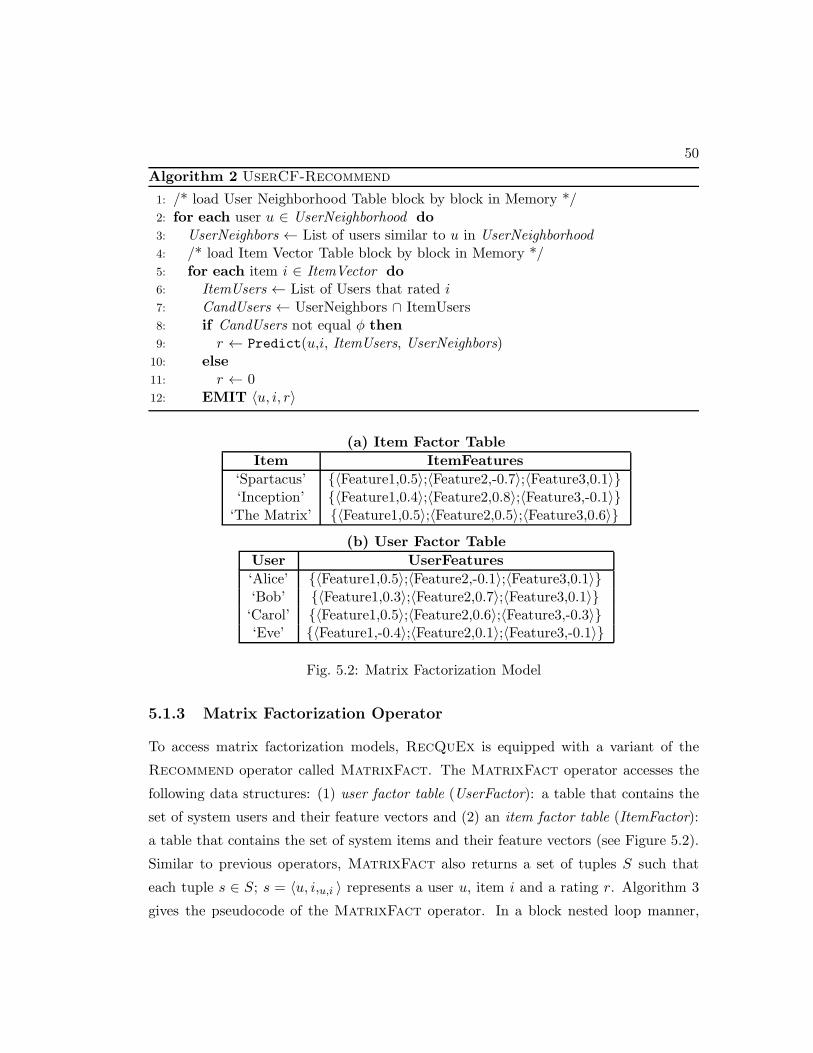
50

Algorithm 2 UserCF-Recommend

1: /* load User Neighborhood Table block by block in Memory */2: for each user u ∈ UserNeighborhood do3: UserNeighbors ← List of users similar to u in UserNeighborhood4: /* load Item Vector Table block by block in Memory */5: for each item i ∈ ItemVector do6: ItemUsers ← List of Users that rated i7: CandUsers ← UserNeighbors ∩ ItemUsers8: if CandUsers not equal φ then9: r ← Predict(u,i, ItemUsers, UserNeighbors)

10: else11: r ← 012: EMIT 〈u, i, r〉

(a) Item Factor Table

Item ItemFeatures

‘Spartacus’ {〈Feature1,0.5〉;〈Feature2,-0.7〉;〈Feature3,0.1〉}‘Inception’ {〈Feature1,0.4〉;〈Feature2,0.8〉;〈Feature3,-0.1〉}‘The Matrix’ {〈Feature1,0.5〉;〈Feature2,0.5〉;〈Feature3,0.6〉}

(b) User Factor Table

User UserFeatures

‘Alice’ {〈Feature1,0.5〉;〈Feature2,-0.1〉;〈Feature3,0.1〉}‘Bob’ {〈Feature1,0.3〉;〈Feature2,0.7〉;〈Feature3,0.1〉}‘Carol’ {〈Feature1,0.5〉;〈Feature2,0.6〉;〈Feature3,-0.3〉}‘Eve’ {〈Feature1,-0.4〉;〈Feature2,0.1〉;〈Feature3,-0.1〉}

Fig. 5.2: Matrix Factorization Model

5.1.3 Matrix Factorization Operator

To access matrix factorization models, RecQuEx is equipped with a variant of the

Recommend operator called MatrixFact. The MatrixFact operator accesses the

following data structures: (1) user factor table (UserFactor): a table that contains the

set of system users and their feature vectors and (2) an item factor table (ItemFactor):

a table that contains the set of system items and their feature vectors (see Figure 5.2).

Similar to previous operators, MatrixFact also returns a set of tuples S such that

each tuple s ∈ S; s = 〈u, i,u,i 〉 represents a user u, item i and a rating r. Algorithm 3

gives the pseudocode of the MatrixFact operator. In a block nested loop manner,

51

Algorithm 3 MatrixFact-Recommend

1: /* load User Features Table block by block in Memory */2: for each user u ∈ UserFactorVector do3: uFeatures ← List of latent factors (features) learned for user u4: /* load Item Features Table block by block in Memory */5: for each item i ∈ ItemFactorVector do6: iFeatures ← List of latent factors (features) learned for item i7: ru,i ← DotProduct(iFeatures, uFeatures)8: EMIT 〈u, i, ru,i〉

MatrixFact scans UserFactor block by block to fetch the feature vector of each user

u. Then, MatrixFact scans ItemNeighborhood block by block to retrieve the feature

vector for each item i. If an item i is already rated by u, we set ru,i to the rating that u

already assigned to i. The algorithm calculates the dot product of both uFeatures and

iFeature and that represents the value of the predicted rating ru,i. ItemCF emits the

tuple 〈u, i, ru,i〉 up in the query pipeline.

5.2 Query Pipeline Integration

The Recommend operators are non-blocking (pipeline-able) database operators that

follows the iterator model adopted by almost all existing relational database engines

(i.e., PostgreSQL in our case). The non-blocking nature means that other operators in

the query pipeline can receive results from the Recommend operator before it is done

with all of its predictions. Being a pipeline-able operator allows a seamless integration

with other query operators in a database query processor. However, as theRecommend

operator only applies to a recommender and does not apply to normal database relations,

it should always be pushed down to the bottom of the query pipeline. In this section, we

discuss the integration of the Recommend operator in the bottom of a query pipeline

with selection, join, and ranking operators.

5.2.1 Selection

Two cases might happen when a selection predicate is applied to the recommendation

answer: (1) Case 1: uid or iid selection predicate, where the selection predicate is applied

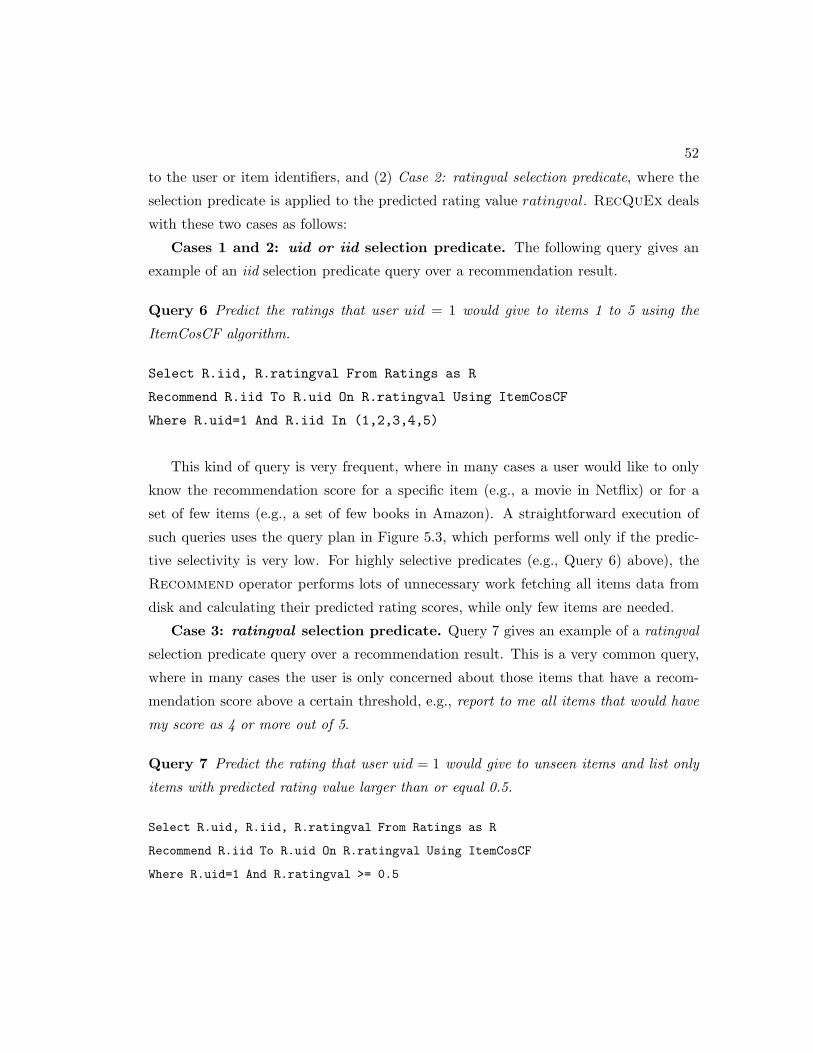
52

to the user or item identifiers, and (2) Case 2: ratingval selection predicate, where the

selection predicate is applied to the predicted rating value ratingval. RecQuEx deals

with these two cases as follows:

Cases 1 and 2: uid or iid selection predicate. The following query gives an

example of an iid selection predicate query over a recommendation result.

Query 6 Predict the ratings that user uid = 1 would give to items 1 to 5 using the

ItemCosCF algorithm.

Select R.iid, R.ratingval From Ratings as R


Where R.uid=1 And R.iid In (1,2,3,4,5)

This kind of query is very frequent, where in many cases a user would like to only

know the recommendation score for a specific item (e.g., a movie in Netflix) or for a

set of few items (e.g., a set of few books in Amazon). A straightforward execution of

such queries uses the query plan in Figure 5.3, which performs well only if the predic-

tive selectivity is very low. For highly selective predicates (e.g., Query 6) above), the

Recommend operator performs lots of unnecessary work fetching all items data from

disk and calculating their predicted rating scores, while only few items are needed.

Case 3: ratingval selection predicate. Query 7 gives an example of a ratingval

selection predicate query over a recommendation result. This is a very common query,

where in many cases the user is only concerned about those items that have a recom-

mendation score above a certain threshold, e.g., report to me all items that would have

my score as 4 or more out of 5.

Query 7 Predict the rating that user uid = 1 would give to unseen items and list only

items with predicted rating value larger than or equal 0.5.

Select R.uid, R.iid, R.ratingval From Ratings as R


Where R.uid=1 And R.ratingval >= 0.5

53

Figure 5.3(a) gives the query plan of the above query, where we first apply the

Recommend operator on the given recommender. Then, the recommender operator

output is fed to a selection operator with the predicate R.ratingval ≥ 0.5 to filter out

those items that do not contribute to the final answer.

5.2.2 Join

Query 8 in Section 5.2 gives an example of a recommendation query, where the output

of the recommender operator needs to be joined with another query to get the movie

names instead of their identifiers and to only retrieve Action movies. This is a very

common query in any recommender system. For example, Netflix and Amazon always

return the item information, not the item identifiers. Also, a Netflix user may opt to

receive movie recommendation for a certain movie genre.

Query 8 Predict the rating that user (uid = 1) would give to action movies.

Select R.uid, M.name, R.ratingval

From Ratings as R, Movies as M


Where R.uid=1 And M.iid = R.iid And M.genre=’Action’

Figure 5.3(b) gives the query plan of the above query, where the ItemCF-

Recommend operator is applied directly to the GeneralRec recommender. In the

meantime, the Movies table goes to a selection operator (i.e., filter) with the pred-

icate “genre=’Action’” to pass only action movies. The output of the Recommend

operator is joined with the output of the selection operator using a traditional join

operator with the predicate ”Movies.iid = GeneralRec.iid” to come up with the movie

names for action movies along with ratings produced from GeneralRec.

5.2.3 Ranking

Query 9 gives an example of a ranking query where we need to return only the top-10

recommended items. This is a very important query as it is very common to return to

the user a limited number of recommended items rather than all items with their scores.

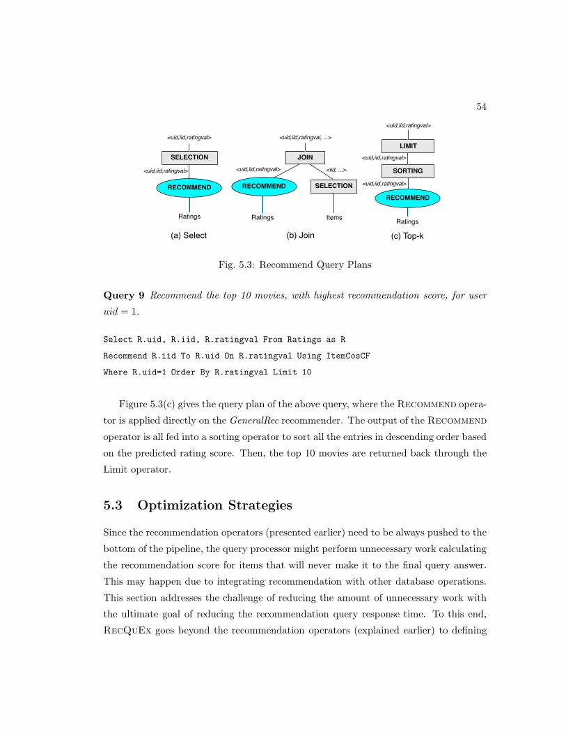
54

Ratings

(c) Top-k

SORTING

<uid,iid,ratingval>

LIMIT

Ratings

<uid,iid,ratingval>

Items

<iid, ...>

JOIN

(b) Join

<uid,iid,ratingval, ...>

SELECTION

<uid,iid,ratingval>

(a) Select

SELECTION

Ratings

<uid,iid,ratingval>

<uid,iid,ratingval>

<uid,iid,ratingval>RECOMMEND RECOMMEND

RECOMMEND

Fig. 5.3: Recommend Query Plans

Query 9 Recommend the top 10 movies, with highest recommendation score, for user

uid = 1.

Select R.uid, R.iid, R.ratingval From Ratings as R


Where R.uid=1 Order By R.ratingval Limit 10

Figure 5.3(c) gives the query plan of the above query, where the Recommend opera-

tor is applied directly on the GeneralRec recommender. The output of the Recommend

operator is all fed into a sorting operator to sort all the entries in descending order based

on the predicted rating score. Then, the top 10 movies are returned back through the

Limit operator.

5.3 Optimization Strategies

Since the recommendation operators (presented earlier) need to be always pushed to the

bottom of the pipeline, the query processor might perform unnecessary work calculating

the recommendation score for items that will never make it to the final query answer.

This may happen due to integrating recommendation with other database operations.

This section addresses the challenge of reducing the amount of unnecessary work with

the ultimate goal of reducing the recommendation query response time. To this end,

RecQuEx goes beyond the recommendation operators (explained earlier) to defining

55

Ratings

INDEXRECOMMEND

(c) IndexRecommend

LIMIT

Ratings

Table

<iid, ...>

JOINRECOMMEND

(b) JoinRecommend

SELECTION

(a) FilterRecommend

Ratings

FILTERRECOMMEND

<uid,iid,ratingval>

<uid,iid,ratingval,...> <uid,iid,ratingval,...>

<uid,iid,ratingval>JOIN

Table

SELECTION

Fig. 5.4: Optimized Recommend Query Plans

more sophisticated operators for common recommender functionality, e.g., top-k recom-

mendation, and joining with other tables. Although such functionality can be simply

expressed using any of the Recommend operators, as described in Section 5.1, it would

be more efficient to have specialized query operators for such common queries. This sec-

tion discusses a major part of RecQuEx query optimizer, which is composed of a set of

recommender-aware operators that correspond to common recommender functionalities.

5.3.1 Selection Optimization

A straightforward execution of queries that combines recommendation and selection

employs the query plan in Figure 5.3(a), which performs well only if the predicate

selectivity is very low. For highly selective predicates (e.g., Query 6), the aforementioned

Recommend operators perform lots of unnecessary work fetching all items data from

disk and calculating their predicted rating scores, while only few items are needed.

Since in many cases, the predicate selectivity is very high; It is very common to

generate recommendation for a single user or predict the rating for only one item, Rec-

QuEx employs a variant of the Recommend operator, called FilterRecommend.

Instead of calculating the predicted rating scores for all user/item pairs, the family of

FilterRecommend operators takes the filtering predicate as input and prunes the pre-

dicted rating score calculation for those items that do not satisfy the filtering predicate.

To achieve that, we modify Algorithms 5 to iterate and calculate the recommendation

only for items that satisfy the uid/iid selection predicate.

56

Item 1 Item 2 Item m. . . Item m-1Item 3

User 2 User n. . .

User 1

User 1

B+-Tree

User 2

B+-Tree

User n

B+-Tree

. . .

Fig. 5.5: RecScore Index Structure

5.3.2 Join Optimization

The straightforward plan for executing queries that combine recommendation and join

(Figure 5.3b) may be acceptable only if there is no filter over the joined relation, or the

filter has very low selectivity. Otherwise, if the filter is highly selective, theRecommend

operators will end up doing redundant work predicting the rating scores for all user/item

pairs, while only few of them are needed. It is very common to have a very selective

filter over the items table, e.g., only Action movies.

To efficiently support such queries, RecQuEx employs the JoinRecommend oper-

ator. Besides the user u and a recommender R, the JoinRecommend operator takes a

joined database relation rel (e.g., Movies) as input, combines their tuples, and returns

the joined result. Analogous to index nested loop join, JoinRecommend employs the

input relation rel as the outer relation. For each retrieved tuple tup ∈ rel, the algorithm

calculates the predicted rating score for item i with iid equal to tup.iid in the same way

it was calculated in the Recommend algorithm (Algorithm 5). The algorithm then con-

catenates 〈uid,iid,ratingval〉 and tup and the resulting joined tuple 〈tup,iid,ratingval〈

is finally added to the join answer S. The algorithm terminates when there are no more

tuples left in rel. Figure 5.4b gives the query plan for Query 8, when employing the

JoinRecommend operator.

5.3.3 Optimization through Pre-Computation

Recommendation applications are rather interactive and real time in nature which neces-

sitates mitigating the recommendation generation latency. To further optimize query

57

execution performance, RecQuEx pre-computes the predicted ratings for user/item

pairs and save them in a data structure, named RecScoreIndex.

Data Structure. RecScoreIndex (see Figure 5.5) is basically a hash table where

each entry is represented by 〈u,RecTreeu〉, as the user identifier and a pointer to a B+-

tree that indexes the pre-computed predicted rating scores of all items unseen by the

user. The predicted rating scores are pre-computed based upon the recommendation

model RecModel trained using the recommender algorithm. Rectreeu is built for each

user u, where the predicted rating score ratingval is the key Rectreeu leaf nodes contain

pointers to the corresponding items. That means that items in the leaf nodes of Rectreeu

are sorted in a descending order of their predicted rating value.

Operator. RecQuEx accesses RecScoreIndex using an optimized recommenda-

tion operator, named IndexRecommend. The optimized operator reduces the amount

of work performed by the recommendation operators by directly accessing the pre-

computed predicted rating scores saved in RecScoreIndex. Algorithm 4 gives the pseu-

docode of the IndexRecommend query operator. Besides the ratings table, the al-

gorithm takes as input a user predicate (uPred), item predicate (iPred), and ratingval

predicate (rPred). The algorithm runs in three main phases: (1) Phase I: User ID

Filtering: In this phase, IndexRecommend fetches each user u that satisfies uPred by

looking up the given user IDs in the RecScoreIndex hash table. (2) Phase II: Rating

Value Filtering: In this phase, IndexRecommend traverses the RecTreeu correspond-

ing to each user u retrieved in the first phase to satisfy the ratingVal predicate rPred

(3) Phase III: Item ID Filtering: In this phase, the algorithm fetches items one-by-one

in the leaf level of RecTreeu. The algorithm filters out those items that do not satisfy

the item predicate (iPred). Finally, IndexRecommend emits each tuple 〈u,i,ru,i〉 that

passes the three phases up in the query pipeline.

Query 10 needs to join the GeneralRec recommender with the Movies table to

only select Action movies and then return the top 5 Action movies to user 1. The

following two plans are deemed correct: (1) Apply the JoinRecommend operator on

recommender GeneralRec and table Movies first and then perform a traditional top-k

operation on the join result. (2) If a RecScoreIndex is maintained, the system may apply

the IndexRecommend operator to retrieve items in sorted order and then perform the

join operation on the returned items to retrieve Action movies (see Plan in Figure 5.4c).

58

Algorithm 4 IndexRecommend

1: /* Phase I: Retrieve Users One by One in RecScoreIndex*/

2: for each user u ∈ RecScoreIndex that satisfies uPred do3: RecTreeu ← Fetch user u RecTree pointer4: /* Phase II: Traverse RecTree to satisfy the ratingval predicate rPred */

5: TreeNode←Traverse(RecTreeu,rPred)6: /* Phase III: Fetch Items One by One at the leaf nodes of RecTreeu */

7: for each item i ∈ FetchNextItem(TreeNode) do8: if item i satisfies iPred then9: ru,i ← the predicted Rating of i stored in the node

10: EMIT 〈u, i, ru,i〉

Query 10 Recommend the top 5 Action movies to user uid = 1 using the SVD Algo-

rithm.

Select M.name, R.ratingval

From Ratings as R, Movies M

Recommend R.iid To R.uid On R.ratingval Using SVD

Where R.uid=1 And M.iid=R.iid And M.genre=’Action’

Order By R.ratingval Desc Limit 5

5.3.4 Scalability

Most recommendation applications (e.g., Amazon, Google News) deal with large user

base and large pool of items. For the system to scale up, i.e., accommodate more

users and items, it must minimize the maintenance cost and reduce the overall storage

occupied by the recommender data structure. Maintaining the RecScoreIndex every

time maintenance is triggered for RecModel exhibits the lowest query response time

because each incoming recommendation query may directly access the pre-computed

recommendation scores stored in RecScoreIndex. However, the maintenance cost as well

as the storage overhead incurred by materializing all RecScoreIndex entries may lead to

a severe scalability bottleneck, especially with large amounts of user/item pairs.

Main idea. Since recommendation queries are personalized for each user, the sys-

tem collects statistics about the demand of each user, and leverages these statistics to

take the materialization decision. RecQuEx stores those 〈user,item,ratingval〉 triplets

59

in RecScoreIndex that correspond to highly demanding users. That mitigates the over-

all recommendation generation latency as queries directly access the pre-computed pre-

dicted ratings in RecScoreIndex. Since the generated recommendation represents a set

of items, the system also collects statistics that quantifies each item’s consumption

rate. The system then determines whether an item is highly consumed, i.e., frequently

rated/updated, and only maintains entries in RecScoreIndex that correspond to those

highly-consumed items.

Statistics

To take the materialization decision, RecQuEx maintains the following statistics for

each created recommender T : (1) Users Histogram: A hash table indexed by the user ID

that contains the following fields for each user u ∈ U : (a) Queries Count (QCu): repre-

sents the number of issued recommendation queries by u since T is created. (b) Query

TimeStamp TSu: time stamp of the last recommendation query issued by u. (c) User

Demand Rate (Du): represents the rate of queries issued by user u. (2) Items Histogram:

A table hashed by the item ID and contains the following fields for each item i: (a) Up-

dates Count UCi: represents the number of updates applied, i.e., ratings insertion, to

item i in recommender T since the recommender is created. (b) Update TimeStamp

TSi: time stamp of the last update transaction performed over item i, (c) Item Con-

sumption rate (Pi): represents the rate of updates performed on item i. (3) Maximum

User Demand (DMAX): the maximum user demand rate Du of a user u among all

users in recommender T . (4) Maximum Item Consumption (PMAX): the maximum

item consumption rate Pi of an item i among all items in recommender T .

Caching Algorithm

Using the statistics maintained for a recommender T , the main role of the cache manager

is determining which user/item/rating triplets need to be cached in RecScoreIndex. To

achieve this goal, the cache manager runs asynchronously every fixed period of time

(e.g., 5 mins) in the background and performs the following steps:

STEP 1: Statistics Maintenance. It first retrieves the set of users U ′ such that

each user u ∈ U ′ has (TSu) larger than the last time the cache manager was invoked.

We also retrieve the set of items I ′ such that each item i ∈ I ′ has (TSi) larger than

60

Algorithm 5 Caching Algorithm

1: Function CacheManager (Recommender T )2: U ′ ← All users in recommender T with TSu larger than TSmat

3: I ′ ← All items in recommender T with TSi larger than TSmat

/* STEP 1: Statistics Maintenance */4: for each item i ∈ I ′ do5: Maintain Pi ← UCi / (TSnow − TSinit)6: If Pi>PMAX then Maintain PMAX←Pi

7: for each user u ∈ U ′ do8: Maintain Pi ← QCu / (TSnow − TSinit)9: If Du>DMAX then Maintain DMAX←Du

/* STEP 2: Materialization Decision */10: for each user/item pair {u,i} ∈ {U ′×I ′} do11: if i is unseen by u then12: Hotu,i ← (Du/DMax) × (Pi/PMax)13: if Hotness Ration Hotu,i ≥ HOTNESS-THRESHOLD then14: Append user/item pair {u,i} to Admission List15: else16: Append user/item pair {u,i} to Eviction List

the last time the cache manager was executed. The cache manager then calculates User

Demand Rate Du for each user u ∈ U ′, as follows: Du = QCu

TSnow−TSinit; such that TS

represents the current system timestamp. In addition, RecDB maintains Maximum

Demand by setting DMAX to Du in case Du value is larger than current DMAX value.

Therefore, the materialization manager calculates Item Consumption Rate Pi for each

item i ∈ I ′, as follows: Pi =UCi

TSnow−TSinit; such that TS represents the current system

timestamp. The system also maintains Maximum Demand by setting PMAX to Pi if Pi

value is larger than current PMAX .

STEP 2: Decision Making. This step leverages the maintained statistics to

decide whether the entry corresponding to a user/item pair needs to be materialized.

To this end, the cache manager maintains two in-memory lists: (1) Admission List:

a list that contains the user/item pairs that require materialization, and (2) Eviction

List: a list that contains those user/item pairs that need to be dematerialized. For

each user/item pair {u,i} such that u ∈ U ′ and i ∈ I ′, we calculate the hotness ratio

Hotu,i (0 ≥ Hotu,i ≤ 1), as follows: Hotu,i = Du

DMax× Pi

PMax; such that Du

DMaxand

61

Users Histogram

User QCu TSu Du

Alice 100 10 100/(15-10)= 20Bob 10 12 10/(15-10)≈ 2

Items Histogram

Item UCi TSi Pi

Spartacus 1000 12 1000/(15-10)≈ 200Inception 10 12 10/(15-10)≈ 2The Matrix 100 10 100/(15-10)= 20

User/Item Pair Hotness Ratio

User u Item i Hotu,iAlice Spartacus (20/20) × (200/200) = 1Alice Inception (20/20) × (2/200) = 0.01Alice The Matrix 20/20 × (20/200) 0.01Bob Spartacus (2/20) × (200/200) 0.1Bob Inception (2/20) × (2/200) = 0.001Bob The Matrix (2/20) × (20/200) ≈ 0.01

Table 5.1: Materialization Manager Example

Pi

PMaxrepresent the normalized user demand rate and item consumption rate, respec-

tively. The hotness ratio Hotu,i determines whether the entry, corresponding to {u,i},

is eligible for materialization. If Hotu,i is greater than or equal to a system parameter

HOTNESS-THRESHOLD (value between 0 and 1), we add the user/item pair {u,i} to the

admission list, otherwise we append them to the eviction list. The HOTNESS-THRESHOLD

exhibits a tradeoff between: (1) Query latency, and (2) System Scalability (Storage

Overhead and Maintenance Cost). In other words, when HOTNESS-THRESHOLD is equal

to 0, RecDB tends to fully materialize all RecScoreIndex entries, and when set to 1,

RecScoreIndex is not materialized at all.

RecScoreIndex Maintenance. When maintenance is triggered for RecModel, the

system retrieves all user/item pairs in the Eviction List and batch deletes all corre-

sponding entries in RecScoreIndex. The system also retrieves the user/item pairs in the

Admission List and batch inserts them in RecScoreIndex. Finally, RecDB maintains

the recommendation score RecScore for all materialized entries.

62

Example. Table 5.1 depicts an example that illustrated the materialization man-

ager dynamics triggered for a cell C. The table gives Cell C Users Histogram and Items

Histograms at the time the materialization manager is invoked at timestamp 15. As

it turns out from the table, Users Histogram contains two users: Alice and Bob, and

Items Histogram contains three items (i.e., Movies): Spartacus, Inception, and The Ma-

trix. The User Demand for Alice is calculated as DAlice = QCAlice / (15-TSAlice = 20).

Similarly, DBob is equal to ≈ 3.33. The item consumption rate PSpartacus for Sparta-

cus movie is evaluated as UCSpartacus / (15-10) = ≈ 200), and the same calculation is

applied to other movies. Table 5.1 also manifests the hotness ratio calculated by the

materialization manager for the user/item pairs. Assume that all movies are unseen

by both Alice and Bob and RecScoreIndex only contains the entry t1 that corresponds

to user Bob and movie Inception. Let HOTNESS-THRESHOLD be set to 0.5, in this case

the entry t1 is added to cell C Eviction List as HotBob,Inception =≈ 0.001 is less than

HOTNESS-THRESHOLD. In contrast, entry t2, corresponding to user Alice and movie Bob,

is added to the Admission List.


This section presents a comprehensive experimental evaluation of RecQuEx based

on an actual system implementation [39] and integration with PostgreSQL 9.2. All

proposed operators are implemented using the iterator model adopted by PostgreSQL

for operator implementations. We evaluate RecQuEx using two real datasets described

as follows: (1) MovieLens: a real movie recommendation dataset [54] that consists of

6040 users, 3883 movies, and one million (1M) ratings. Each movie has name and

genre attributes. The ratings data contains historical ratings (in a scale from 1 to 5)

that users have assigned to movies. (2) Foursquare: a real venue (e.g., restaurant)

recommendation dataset extracted [55] from Foursquare website, and consists of 150K

users, 90K venues, and 1M ratings. Each user has a spatial location that represents

where that user lives. Each item has also a spatial location.

We run our experiments for the following five popular recommendation algorithms,

all supported by RecQuEx : (1) ItemCosCF: Item-Item Collaborative Filtering (CF)

63

0

0.2

0.4

0.6

0.8

1

1.2

1 2 3 4 5 6 7 8 9 10

Resp

on

se T

ime (

sec)

Data SIze (* 105)

RecFiltRec

(a) ItemCosCF

0

0.2

0.4

0.6

0.8

1

1.2

1.4

1 2 3 4 5 6 7 8 9 10

Resp

on

se T

ime (

sec)

Data Size (* 105)

RecFiltRec

(b) UserPearCF

0

0.05

0.1

0.15

0.2

0.25

0.3

1 2 3 4 5 6 7 8 9 10

Resp

on

se T

ime (

sec)

Data Size (* 105)

RecFiltRec

(c) SVD

Fig. 5.6: Selection: Varying Data Size (MovieLens)

with cosine distance used to measure similarity among items. (2) ItemPearCF: item-

item CF with pearson correlation similarity measure. (3) UserCosCF: user-user CF

with cosine distance similarity. (4) UserPearCF: user-user CF with pearson correlation

similarity. (5) SVD: Regularized Gradient Descent Singular Value Decomposition.

All experiments were performed on a machine with 3.6 Ghz Quad-Core processor,

16 GB RAM, 500 GB storage, and running Ubuntu Linux 12.04. The default dataset

is MovieLens.

5.4.1 Recommender Queries

In this section, we evaluate the query execution performance in terms of the query re-

sponse time. We consider the following four different approaches for query execution

that are applied only when possible: (1) Rec: a query plan that only relies on the

Recommend operator to execute recommendation queries (Figure 5.3). (2) FiltRec: a

query plan that leverages the FilterRecommend operator to optimize recommenda-

tion queries with a predicate over iid (Figure 5.4(a)). (3) IndRec: a plan that exploits

the IndexRecommend operator as well as the RecScoreIndex to either (a) process a rec-

ommendation query with a predicate over RecScore (see Figure 5.4(b)), or (b) execute

a ranking (Top-k) query (Figure 5.4(d)). (4) JoinRec: a plan that employs the Join-

Recommend operator to join a recommendation with a database table (Figure 5.4(c)).

For space constraints, we plot only the results of three recommendation algorithms,

namely, ItemCosCF, UserPearCF, and SVD.

64

0.2

0.4

0.6

0.8

1

1.2

1.4

.1 .2 .3 .4 .5 .6 .7 .8 .9 1

Resp

on

se T

ime (

sec)

% of Results

RecFiltRec

(a) ItemCosCF

0.2

0.4

0.6

0.8

1

1.2

1.4

1.6

.1 .2 .3 .4 .5 .6 .7 .8 .9 1

Resp

on

se T

ime (

sec)

% of Results

RecFiltRec

(b) UserPearCF

0

0.05

0.1

0.15

0.2

0.25

0.3

0.35

.1 .2 .3 .4 .5 .6 .7 .8 .9 1

Resp

on

se T

ime (

sec)

% of Results

RecFiltRec

(c) SVD

Fig. 5.7: Selection: Varying Selectivity (MovieLens)

Selection: iid Predicate (Query 6)

In this section, we study the performance of recommendation queries with selection

predicate applied to the recommender iid field (e.g., Query 6 in Section 5.3.1). Unless

mentioned otherwise, the query selectivity is set to 25% and the data size is 1M ratings.

Varying data size. Figure 5.6 studies the impact of data size on the query execu-

tion performance. We vary the data size from 100K to 1M ratings, executing a set of 100

synthetically generated queries using ItemCosCF, UserPearCF, and SVD recommenda-

tion algorithms. For all recommender algorithms, FiltRec outperforms Rec by at least

an order of magnitude. This is obvious since FiltRec applies the iid filtering predicate

before calculating the predicted recommendation score for an item, which saves a huge

amount of effort wasted by Rec in applying the Recommend operator first on all items

and then performing the predicate filtering step. In the meantime, the query response

time increases as the data size gets bigger since we need to retrieve more recommenda-

tion model entries in ItemCosCF and UserPearCF. In the SVD case, the response time

remains unchanged.

Varying Selectivity. Figure 5.7 gives the impact of iid predicate selectivity on the

average query response time. As it turns out from the figure, as we increase the per-

centage of reported items (decrease selectivity), the average query response time in Rec

remains constant since the Recommend operator predicts the recommendation score

for all items anyway before applying the iid predicate. On the other hand, FiltRec query

response time increases linearly with the percentage of reported items until it reaches

the same performance as Rec when 100% of items are reported. That happens because

65

0.5

1

1.5

2

2.5

3

3.5

4

1 2 3 4 5 6 7 8 9 10

Resp

on

se T

ime (

sec)

Data Size (*105)

JoinJoinRec

(a) ItemCosCF

0.5 1

1.5 2

2.5 3

3.5 4

4.5

1 2 3 4 5 6 7 8 9 10

Resp

on

se T

ime (

sec)

Data Size (*105)

JoinJoinRec

(b) UserPearCF

1.5 2

2.5 3

3.5 4

4.5 5

5.5 6

6.5

1 2 3 4 5 6 7 8 9 10

Resp

on

se T

ime (

sec)

Data Size (*105)

JoinJoinRec

(c) SVD

Fig. 5.8: Join: Joined Recommender Data Size (Foursquare)

0

5

10

15

20

25

30

35

40

.1 .2 .3 .4 .5 .6 .7 .8 .9 1

Resp

on

se T

ime (

sec)

% of Results

JoinJoinRec

(a) ItemCosCF

0 5

10 15 20 25 30 35 40 45

.1 .2 .3 .4 .5 .6 .7 .8 .9 1

Resp

on

se T

ime (

sec)

% of Results

JoinJoinRec

(b) UserPearCF

0

10

20

30

40

50

60

70

.1 .2 .3 .4 .5 .6 .7 .8 .9 1

Resp

on

se T

ime (

sec)

% of Results

JoinJoinRec

(c) SVD

Fig. 5.9: Join: Joined Table (rel) Selectivity (Foursquare)

FiltRec, when 100% of items are returned, performs the same amount of recommenda-

tion score calculation as Rec. However, for higher selectivity (i.e., lower % of results),

FiltRec outperforms Rec by more than an order of magnitude. With iid selection, a typ-

ical selectivity would be very high, i.e., less than 1%, which shows better performance

for FiltRec over Rec.

Join (Query 8)

This section studies the performance of recommendation queries that involve joining

the recommendation answer with other database tables in the Foursquare dataset (e.g.,

Query 8 in Section 5.2). The joined table has a selection predicate that filters out un-

wanted items. Unless mentioned otherwise, the selectivity for the join selection predicate

is set to 25% and the data size is 1M ratings.

Varying data size. In this experiment, we build recommenders with different data

sizes (100K to 1M ratings), and we generate a workload of 100 join queries that join

the created recommender and the movies table. Figure 5.8 shows that JoinRec scales

66

0

0.2

0.4

0.6

0.8

1

1.2

1.4

1 2 3 4 5 6 7 8 9 10

Resp

on

se T

ime (

sec)

Data Size (*105)

RecIndRec

(a) ItemCosCF

0

0.2

0.4

0.6

0.8

1

1.2

1.4

1 2 3 4 5 6 7 8 9 10

Resp

on

se T

ime (

sec)

Data Size (* 105)

RecIndRec

(b) UserPearCF

0

0.05

0.1

0.15

0.2

0.25

0.3

1 2 3 4 5 6 7 8 9 10

Resp

on

se T

ime (

sec)

Data Size (* 105)

RecIndRec

(c) SVD

Fig. 5.10: Ranking: Varying Data Size (MovieLens)

0.01

0.1

1

10

1 2 3 4 5 6 7 8 9 10

Resp

on

se T

ime (

sec)

Limit (* 102)

RecIndRec

(a) ItemCosCF

0.01

0.1

1

10

1 2 3 4 5 6 7 8 9 10

Resp

on

se T

ime (

sec)

Limit (* 102)

RecIndRec

(b) UserPearCF

0.001

0.01

0.1

1

1 2 3 4 5 6 7 8 9 10

Resp

on

se T

ime (

sec)

Limit (* 102)

RecIndRec

(c) SVD

Fig. 5.11: Ranking: Varying Limit (k) Size (MovieLens)

about an order of magnitude better than Join for all recommendation algorithms. The

main reason is that JoinRecommend efficiently calculates the predicted score only for

filtered items. In the meantime, the bigger the data size, the worse the query execution

performance for both Join and JoinRec, since more data are joined. That happens for

all recommendation algorithms, except for SVD.

Varying Selectivity. In these experiments, we vary the selectivity of the joined

table with the input recommender. We generate a workload of 100 random join queries

of the same selectivity, and execute such queries for each recommendation algorithm.

We simulate the selectivity change in terms of the ratio of output tuples (filtered by a

selection predicate) over the original number of tuples in the joined table rel. Figure 5.9

shows that JoinRec exhibits more than an order of magnitude better performance than

Join for high selectivity (small % of rel). However, when the selectivity decreases (%

of rel increases), JoinRec performance becomes closer to Join since JoinRec has to

compute the predicted score for more items.

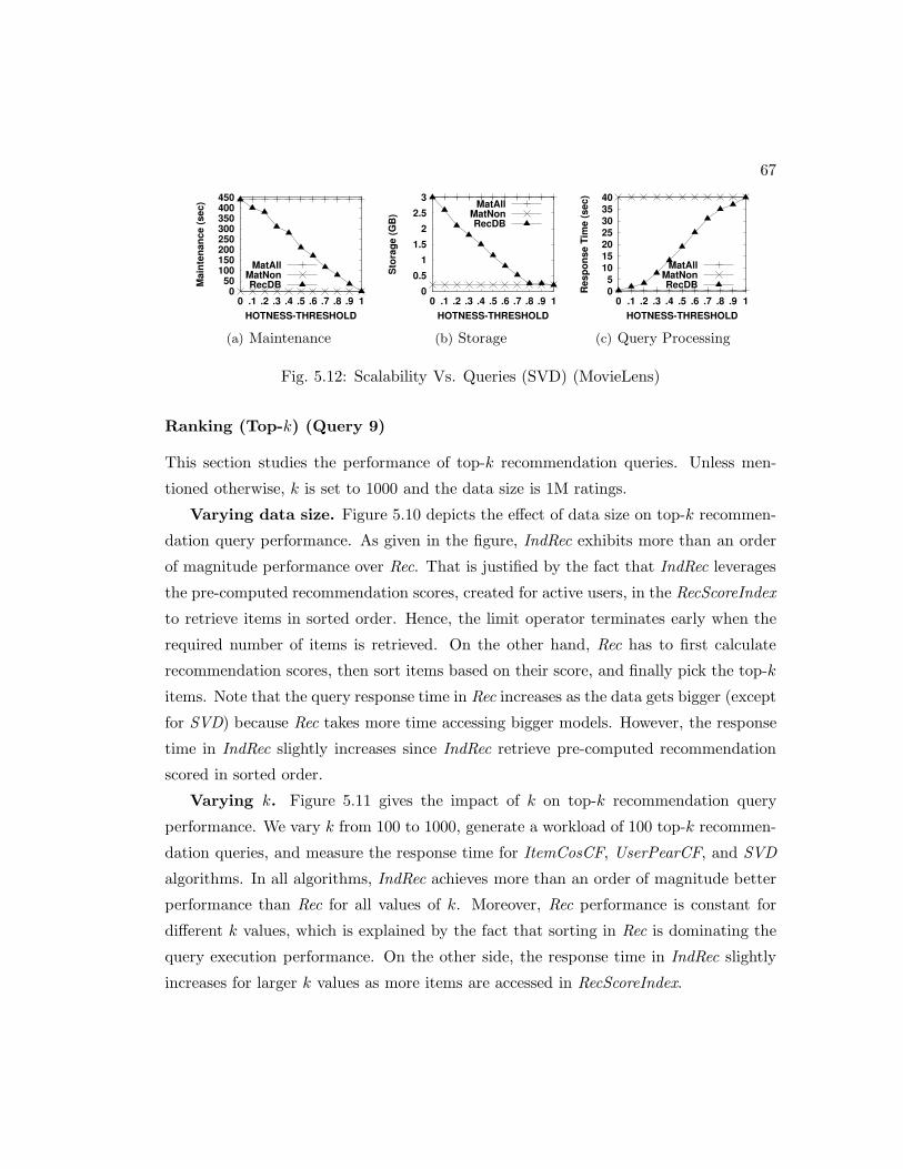
67

0 50

100 150 200 250 300 350 400 450

0 .1 .2 .3 .4 .5 .6 .7 .8 .9 1

Main

ten

an

ce (

sec)

HOTNESS-THRESHOLD

MatAllMatNonRecDB

(a) Maintenance

0

0.5

1

1.5

2

2.5

3

0 .1 .2 .3 .4 .5 .6 .7 .8 .9 1

Sto

rag

e (

GB

)

HOTNESS-THRESHOLD

MatAllMatNonRecDB

(b) Storage

0

5 10

15 20

25 30

35

40

0 .1 .2 .3 .4 .5 .6 .7 .8 .9 1

Resp

on

se T

ime (

sec)

HOTNESS-THRESHOLD

MatAllMatNonRecDB

(c) Query Processing

Fig. 5.12: Scalability Vs. Queries (SVD) (MovieLens)

Ranking (Top-k) (Query 9)

This section studies the performance of top-k recommendation queries. Unless men-

tioned otherwise, k is set to 1000 and the data size is 1M ratings.

Varying data size. Figure 5.10 depicts the effect of data size on top-k recommen-

dation query performance. As given in the figure, IndRec exhibits more than an order

of magnitude performance over Rec. That is justified by the fact that IndRec leverages

the pre-computed recommendation scores, created for active users, in the RecScoreIndex

to retrieve items in sorted order. Hence, the limit operator terminates early when the

required number of items is retrieved. On the other hand, Rec has to first calculate

recommendation scores, then sort items based on their score, and finally pick the top-k

items. Note that the query response time in Rec increases as the data gets bigger (except

for SVD) because Rec takes more time accessing bigger models. However, the response

time in IndRec slightly increases since IndRec retrieve pre-computed recommendation

scored in sorted order.

Varying k. Figure 5.11 gives the impact of k on top-k recommendation query

performance. We vary k from 100 to 1000, generate a workload of 100 top-k recommen-

dation queries, and measure the response time for ItemCosCF, UserPearCF, and SVD

algorithms. In all algorithms, IndRec achieves more than an order of magnitude better

performance than Rec for all values of k. Moreover, Rec performance is constant for

different k values, which is explained by the fact that sorting in Rec is dominating the

query execution performance. On the other side, the response time in IndRec slightly

increases for larger k values as more items are accessed in RecScoreIndex.

68

0

50

100

150

200

250

300

350

0 .1 .2 .3 .4 .5 .6 .7 .8 .9 1

Main

ten

an

ce (

sec)

HOTNESS-THRESHOLD

MatAllMatNonRecDB

(a) Maintenance

0

1

2

3

4

5

6

7

0 .1 .2 .3 .4 .5 .6 .7 ..8 9 1

sto

rag

e (

GB

)

HOTNESS-THRESHOLD

MatAllMatNonRecDB

(b) Storage

1 2 3 4 5 6 7 8 9

10

0 .1 .2 .3 .4 .5 .6 .7 .8 .9 1

Resp

on

se T

ime (

sec)

HOTNESS-THRESHOLD

MatAllMatNonRecDB

(c) Query Processing

Fig. 5.13: Scalability Vs. Queries (ItemCosCF) (MovieLens)

5.4.2 Recommender Storage and Maintenance

In this section, we evaluate the tradeoff between system scalability in terms of stor-

age/maintenance overhead and query processing performance. We vary the value of

HOTNESS-THRESHOLD from 0 to 1 (with an increment of 0.1) and measure the mainte-

nance overhead (Figure 5.12(a) and 5.13(a)), storage cost (Figure 5.12(b) and 5.13(a)),

and query processing performance (Figure 5.12(c) and 5.13(c)). We randomly generate

a 80:20, 50:50, 20:80 query:update workload. We compare RecQuEx with two basic

approaches: (1) MatAll: that maintains all RecScoreIndex entries, and (2)MatNon: that

does not maintain RecScoreIndex at all. For all approaches, we measure the aggregate

maintenance cost (in Seconds), storage overhead (in GBytes), and query response time

for both SVD and ItemCosCF algorithms.

As it turns out from Figures 5.12(a) and 5.13(a), MatAll incurs the highest mainte-

nance overhead due to the fact that MatAll maintains all RecScoreIndex entries. Mat-

Non has the lowest maintenance overhead as it maintains no RecScoreIndex entries. As

HOTNESS-THRESHOLD increases, RecQuEx maintains more RecScoreIndex entries and

hence leads to higher maintenance cost. Figure 5.12(b) and 5.13(a) show that MatAll

occupies the highest storage space since it maintains all RecScoreIndex entries. MatNon

occupies the least storage space due to the fact that it does not maintain RecScor-

eIndex at all. On the other hand, RecQuEx stores more recommendation models for

higher HOTNESS-THRESHOLD values. In Figure 5.12(c) and 5.13(c), MatAll achieves the

best query execution performance since all RecScoreIndex entries are available at query

time whereas the total opposite happens for the MatNon approach. RecQuEx achieves

better query performance as HOTNESS-THRESHOLD decreases.

Chapter 6

RecDB Support for Context

Pre-filtering Recommenders

Classical recommender systems answer traditional context-free recommendation queries

like, Recommend me 10 movies, where recommendation is generated to the querying

user regardless of the context (e.g., user age, job, gender, and location). On the other

side, a context-aware recommender would consider contextual information in producing

recommendation to end-users. For instance, a Context Post-Filtering Recommender

would build a recommendation model M using all users’ opinions history and then filter

the produced recommendation (calculated using PredictRating(u, i)) based on a set of

attributes to answer context-aware recommendation queries like: Recommend me 10

Restaurants that are near by my location. Also, a Context Pre-filtering Recommender

trains the recommendation model M only based on a subset of the users’ opinions that

correspond to specific (filtered) attributes’ range and hence would be able to support

context-aware recommendations queries such as: Recommend me 10 movies that people

my age would like, or Recommend me 5 movies that people that live in my city would like.

From a modeling perspective, it has been shown that such context-aware recommenders

would exhibit higher accuracy than context-free recommendations [34, 35, 56, 57, 58,

59, 60]. Chapter 5 shows how to to generate context post-filtering recommendation

by incorporating the recommendation functionality inside the database system query

69

70

processor. This chapter explains an extension of RecDB that supports context pre-

filtering recommender.

6.1 Context Pre-Filtering Recommender

This section describes how RecDB users creates and query a context pre-filtering rec-

ommender.

6.1.1 Creating a Recommender

To allow creating a new recommender, RecDB employs a new SQL statement, called

CREATE RECOMMENDER, as follows:

CREATE RECOMMENDER [Recommender Name] ON [Ratings Table]

USERS FROM [Users ID Column]

ITEMS FROM [Items ID Column]

RATINGS FROM [Ratings Value Column]

ATTRIBUTES [Attributes Set]

USING [Recommendation algorithm]

The recommender creation SQL is extended to accept the ATTRIBUTES parameter which

represents a set of dimensions that the recommender will be built on (e.g., age). Exam-

ples are given below:

Recommender 4 AgeRec: an age-aware context-prefiltering recommender created on

the input data stored in the Ratings table of Figure 3.2, using the ItemCosCF recom-

mendation algorithm:

Create Recommender AgeRec On Ratings

Users From uid Item From iid Ratings From ratingval

Attributes age Using ItemCosCF

With this SQL, a new recommender, named AgeRec, is added to the database system,

and can be queried later to return a set of recommended movies based on the user age,

e.g., recommend me five movies that people in my age like.

71

Recommender 5 AgeCityGenderRec: an (age, city, gender)-aware recommender cre-

ated on the input ratings table, using the SVD recommendation algorithm:

Create Recommender AgeCityGenderRec On Ratings

Users From uid Item From iid Ratings From ratingval

Attributes age, city, gender Using SVD

With this SQL clause, RecDB creates a new recommender, named AgeCityGenderRec,

that is added it to the database system. This recommender can be queried later to

return to a querying users a set of recommended movies based on the user age, city, and

gender, e.g., recommend me five movies that people in my age, living in my city, and of

my gender, would like.

Notice that in the above two examples, if we had no ATTRIBUTES clause, we would

create a traditional recommender that can be queried to recommend a set of movies for

a certain user, regardless of the user attributes, e.g., recommend me five movies.

6.1.2 Querying a Recommender

Once a recommender is created and registered in RecDB using the CREATE

RECOMMENDER statement, users can issue SQL queries that harnesses the initialized con-

text pre-filtering recommender to produce recommendation to end-users, as follows:

SELECT <Select Clause>

FROM <CFILTER(Ratings Table, Attributes)>

RECOMMEND <UserID> TO <ItemID> ON <RatingVal>

USING <Recommendation Algorithm>

WHERE <Where Clause>

Query Semantics. To access a context pre-filtering recommender, the application

developer has to invoke the CFILTER() function. CFILTER takes the Ratings table and

designated contextual attributes as input and returns a view which consists of tuples in

the ratings table that satisfy the given contextual attributes. An example of a query is

given below:

Query 11 Return the top-10 recommended items to user with ID 1, based on the user

age, city, and gender.

72

Male

Female

18-24 25-34 35-60

Minneapolis

St. Paul

Edina

age

city

gender

RecName

AgeRec

AgeGenderRec

RecIndex

GeneralRec

Ratings Table Attributes

AgeCityGenderRec

AgeCityGenderRec Grid

RecCatalog

.

.

.

age

18-24

25-34

35-60

AgeRec Grid

!

Ratings

Ratings

Ratings

Ratings

N/A

{Age}

{Age, Gender}

{Age, City, Gender}

AgeRec_1824

AgeGenderRec_1824_F

Ratings_Age1824

Ratings_Age1824_GenderF

Ratings

GeneralRec

AgeCityGenderRec_3560

_Minneapolis_M

AgeCityGenderRec_3560

_Edina_M

AgeRec_1824

AgeRec_2534

AgeRec_2534

... ...

N/A

...

N/A

RecModel

... ... ...

Ratings_Age1824

AgeRec_1824

RecModel

. . .

Male

Female

18-24 25-34 35-60

age

gender

AgeGenderRec Grid

.

.

.

AgeGenderRec_3560_M

AgeGenderRec_3560_F

Ratings_Age1824_

GenderF

AgeGenerRec_1824_F

RecModel

. . .

Fig. 6.1: Recommender Grid data structure

Select R.uid, R.iid, R.ratingval

From CFilter(Ratings,age=’18-25’,city=’Minneapolis’,gender=F) as R


Where R.uid=1 Order By R.ratingVal Desc Limit 10

In this case, RecDB uses the AgeCityGenderRec, which was created before using

CREATE RECOMMENDER. Since this recommender was created based on the age attribute,

Query 11 will predict the ratings based on the values of the age attribute value passed

to the CFilter function. The query finally returns the Top-10 movies to user 1 in a

descending order of the predicted rating value (ratingval).

6.2 Data Structure

After creating a context pre-filtering recommender, a main challenge is how to inter-

nally represent, store, and maintain the underlying recommendation models in a scalable

manner. To address this issue, we introduce the following data structures to represent

user-created multidimensional recommenders: (1) We maintain one global structure,

namely RecCatalog, for all created recommenders (section 6.2.1). (2) For each recom-

mender, we maintain one multidimensional grid and we explain how we reduce both

storage and maintenance overhead to achieve scalability (section 6.2.2).

73

6.2.1 Recommender Catalog

RecDB maintains a relational table, termed RecCatalog, that includes metadata about

all created recommenders, and is stored as part of the main database catalog that in-

cludes information about tables, index structures, etc. A row in RecCatalog has seven

attributes: (1) RecName; the recommender name, (2) Users; the input users table,

(3) Items; the input items table, (4) Ratings; the input ratings table, (5) Attributes;

a vector where each element corresponds to an attribute in the users table that con-

tributes to the recommender model, (6) Algorithm; the algorithm used to generate

predicted scores, and (7) RecIndex; a pointer to the multi-dimensional grid index for

this particular recommender. A new row is added/deleted to/from RecCatalog with each

successful CREATE RECOMMENDER / DROP RECOMMENDER SQL statement. Figure 6.1 gives

an example of RecCatalog, where it has four entries for four recommenders, AgeRec,

AgeGenderRec, AgeCityGenderRec, and GeneralRec. With each recommender, the cor-

responding attributes are listed. Notice that in the case of GeneralRec, Attributes is

empty, which corresponds to a general recommender system regardless of any attributes.

6.2.2 Recommender Grid

For each recommender, RecDB maintains a Multi-dimensional Grid G, where each

dimension corresponds to one of the recommender attributes. A grid cell C in G rep-

resents a subdomain of the space created by the multiple attributes. The subdomain

could be a certain value for categorical attributes or range of values for continuous do-

main attributes. For example, as AgeRec recommender in Figure 6.1 is defined based on

only one attribute (age), its index is a one-dimensional grid based on the age attribute.

As this is a continuous domain attribute, each cell represents a range of age values,

i.e., [18-24], [25-34], and [35-60]. In the meantime, the AgeCityGenderRec recommender

index is a three-dimensional grid based on three attributes (age, city, and gender). The

age dimension is divided into three categories based on range of values. The city at-

tribute has three values as {Minneapolis, St. Paul, Edina}, while the gender attribute

is divided into two categorical values as {Male, Female}. The top left outer cell (check

marked in Figure 6.1) in AgeCityGenderRec represents the values 〈18-24, Minneapolis,

Female〉 that correspond to its values of the 〈age, city, gender〉 dimensions.

74

Each cell in the multi-dimensional grid points to a table, RecModel, that maintains

auxiliary precomputed information to speed up the generation of the recommendation

query result. The precomputed information may have different schema based on the

underlying recommendation algorithm. For example, for the Item-Item collaborative fil-

tering algorithm, RecModel represents an items similarity list with the schema (ItemID1,

ItemID2, SimScore), where SimScore is computed.

Initialization. The multi-dimensional grid G is initialized upon issuing a CREATE

RECOMMENDER statement, through two main steps: (1) Grid Construction, where we

allocate the memory space for the grid, and decide on each cell size in terms of the

values it represents. In case of categorical attributes (e.g., Gender, Job, and City),

we allocate one cell per attribute. For continuous domain attributes (e.g., age and

salary), we divide the space into N parts, where parts have almost equal number of

ratings. More sophisticated techniques can be used to divide the space. Yet, we opt

for a simple division here as a proof of concept for RecDB functionality. (2) RecModel

Building, where the RecModel table for each cell C in G is built by running the specified

recommender algorithm in the CREATE RECOMMENDER statement on the set of users U

whose attributes correspond to the subdomain covered by C. For instance, in case of

ItemCosCF recommendation algorithm, we scan the ratings table and run a nested loop

algorithm over all items to calculate the cosine similarity score between every item pair

in each cell C. After the initialization procedure successfully terminates, a pointer to

the newly created grid structure G is added to the RecIndex field corresponding to the

appropriate recommender entry in RecCatalog.

6.2.3 The CFilter Function

CFILTER is a database function that takes as input a ratings table (see Figure 3.2) and

a set of contextual attributes. By specifying the CFILTER in the FROM clause, RecDB

looks into RecCatalog to find an existing context pre-filtering recommender created

on the specified ratings table and contextual attributes. Therefore, CFILTER follows

the index pointer of the RecCatalog entry to fetch the multi-dimensional recommender

grid index, and returns as output the local recommender that matches the specified

contextual attributes. An example is given below:

75

Algorithm 6 CFilter (Ratings R, AttributesAttr)

1: Cat ← RecCatalog entry that corresponds to recommender R2: G ← Cat.RecIndex (The Multi-dimensional Grid Index)3: Attr ← The set of attributes in Cat.Attributes4: AttrV ← Values of attributes Attr in table Cat.Users for uid5: C ← The cell in G that corresponds to AttrV6: return C.ratingV iew

Query 12 Predict the rating that system users would give to unseen items based on the

user age, city, and gender.


From CFilter(Ratings,age=’18-25,city=’Minneapolis’,gender=’Female’) as R


The CFilter finds that the AgeCityGenderRec recommender, registered in the Rec-

Catalog, matches the input contextual attributes, i.e., age, gender, and city. RecDB

thus follows the index pointer of the RecCatalog entry to the three-dimensional rec-

ommender grid index, and retrieves the local recommender grid cell that corresponds

to the specified contextual attributes (18-25 age, Female gender, and ’Minneapolis’

city). CFilter finally returns the name of the ratings view R that consists of all ratings

residing in the local recommender cell, and the query is re-written as follows:


From ratings 1825 Minneapolis Female as R


After applying the CFilter function, RecDB executes the above (re-written) query

using the Recommend operator as described before in Section 5.1.


We evaluate the context pre-filtering recommender creation and initialization process

performance using the following two metrics: (1) Recommender Initialization Time:

the total runtime (in seconds) taken by the system to process a CREATE RECOMMENDER

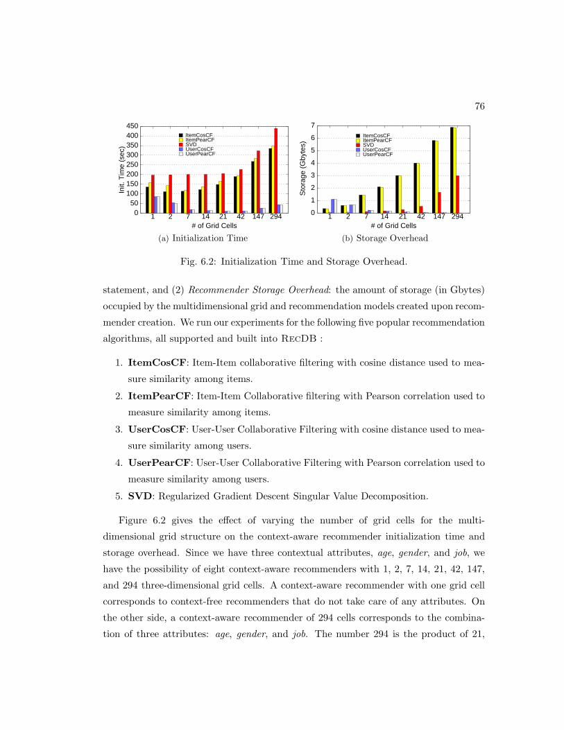
76

Init.

Tim

e (s

ec)

# of Grid Cells

ItemCosCFItemPearCFSVDUserCosCFUserPearCF

0 50

100 150 200 250 300 350 400 450

1 2 7 14 21 42 147 294

(a) Initialization Time

ItemCosCFItemPearCFSVDUserCosCFUserPearCF

0

1

2

3

4

5

6

7

1 2 7 14 21 42 147 294

Sto

rage

(G

byte

s)

# of Grid Cells

(b) Storage Overhead

Fig. 6.2: Initialization Time and Storage Overhead.

statement, and (2) Recommender Storage Overhead: the amount of storage (in Gbytes)

occupied by the multidimensional grid and recommendation models created upon recom-

mender creation. We run our experiments for the following five popular recommendation

algorithms, all supported and built into RecDB :

1. ItemCosCF: Item-Item collaborative filtering with cosine distance used to mea-

sure similarity among items.

2. ItemPearCF: Item-Item Collaborative filtering with Pearson correlation used to

measure similarity among items.

3. UserCosCF: User-User Collaborative Filtering with cosine distance used to mea-

sure similarity among users.

4. UserPearCF: User-User Collaborative Filtering with Pearson correlation used to

measure similarity among users.

5. SVD: Regularized Gradient Descent Singular Value Decomposition.

Figure 6.2 gives the effect of varying the number of grid cells for the multi-

dimensional grid structure on the context-aware recommender initialization time and

storage overhead. Since we have three contextual attributes, age, gender, and job, we

have the possibility of eight context-aware recommenders with 1, 2, 7, 14, 21, 42, 147,

and 294 three-dimensional grid cells. A context-aware recommender with one grid cell

corresponds to context-free recommenders that do not take care of any attributes. On

the other side, a context-aware recommender of 294 cells corresponds to the combina-

tion of three attributes: age, gender, and job. The number 294 is the product of 21,

77

7, and 2, as the number of categories of job, age, and gender attributes, respectively.

Similarly, 147 grid cells correspond to an 〈age, job〉-aware recommender, and so on.

Figure 6.2 shows that the higher the number of grid cells, the higher the initialization

time and storage overhead for the ItemCosCF, ItemPearCF, and SVD recommendation

algorithms. The main reason is that more grid cells lead to building more recommenda-

tion models, as we build one recommendation model per grid cell. This consumes both

storage and computation time. However, the opposite scenario happens for UserCosCF

and UserPearCF algorithms. This counter intuitive behavior is mainly because these

two recommender algorithms partition the user ratings based on the user attributes and

hence, the number of users is small in each cell and building a user similarity list for

several small cells is faster (and requires less storage) than building the user similarity

list for one fat cell. Overall, for all recommender algorithms and number of grid cells,

RecDB is able to provide a reasonable computational and storage overhead.

Comparing various recommender algorithms to each other shows that UserCosCF

and UserPearCF are mostly faster and occupy less storage on disk than ItemCosCF and

ItemPearCF. That happens due to the fact that the number of ratings per user in the

dataset is less than the number of ratings per item. For all created recommenders, SVD

consistently takes more time than other algorithms since SVD is an iterative algorithm

that takes several iterations to build the recommendation model.

Chapter 7

Handling Location-Aware

Recommendation Scenarios

Currently, myriad applications can produce location-based ratings that embed

user and/or item locations. For example, location-based social networks (e.g.,

Foursquare [61] and Facebook Places [62]) allow users to “check-in” at spatial desti-

nations (e.g., restaurants) and rate their visit, thus are capable of associating both user

and item locations with ratings. Such ratings motivate an interesting new paradigm of

location-aware recommendations, whereby the recommender system exploits the spatial

aspect of ratings when producing recommendations. Existing recommendation tech-

niques [6] assume ratings are represented by the (user, rating, item) triple, thus are

ill-equipped to produce location-aware recommendations.

In this Chapter, we propose LARS, a novel location-aware recommender system

built specifically to produce high-quality location-based recommendations in an efficient

manner. LARS produces recommendations using a taxonomy of three types of location-

based ratings within a single framework: (1) Spatial user ratings for non-spatial items,

represented as a four-tuple (user, ulocation, rating, item), where ulocation represents a

user location; (2) non-spatial user ratings for spatial items, represented as a four-tuple

(user, rating, item, ilocation), where ilocation represents an item location, for example,

a user with unknown location rating a restaurant; (3) spatial user ratings for spatial

items, represented as a five-tuple (user, ulocation, rating, item, ilocation), for example, a

78

79

U.S. State Top Movie Genres Avg. Rating

Minnesota Film-NoirWar

Drama

Wisconsin

Florida

3.64.04.03.93.84.34.14.04.0

DocumentaryWar

Film-NoirMysteryRomanceFantansyAnimation

WarMusical

3.63.73.8

(a) Movielens preference locality

Users from: Visited venues in: % Visits

Edina, MN Minneapolis , MN

Edina , MN

Eden Prarie , MN

Robbinsdale, MN Brooklyn Park, MN

Robbinsdale, MN

Minneapolis, MN

Falcon Heights,

MN

St. Paul, MN

Minneapolis, MN

Roseville, MN

37 %

59 %

5 %

32 %

20 %

15 %

17 %

13 %

10 %

(b) Foursquare preference locality

Fig. 7.1: Preference locality in location-based ratings.

user at his/her office rating a restaurant visited for lunch. Traditional rating triples can

be classified as non-spatial ratings for non-spatial items and do not fit this taxonomy.

7.1 A Study of Location-Based Ratings

The motivation for our work comes from analysis of two real-world location-based rat-

ing datasets: (1) a subset of the well-known MovieLens dataset [50] containing approx-

imately 87K movie ratings associated with user zip codes (i.e., spatial user ratings for

non-spatial items) and (2) data from the Foursquare [61] location-based social network

containing user visit data for 1M users to 643K venues across the United States (i.e.,

spatial ratings for spatial items).

Preference locality. Preference locality suggests users from a spatial region (e.g.,

neighborhood) prefer items (e.g., movies, destinations) that are manifestly different

than items preferred by users from other, even adjacent, regions. Figure 7.1(a) lists

the top-4 movie genres using average MovieLens ratings of users from different U.S.

states. While each list is different, the top genres from Florida differ vastly from the

others. Florida’s list contains three genres (“Fantasy”, “Animation”, “Musical”) not in

the other lists. This difference implies movie preferences are unique to specific spatial

regions, and confirms previous work from the New York Times [27] that analyzed Netflix

user queues across U.S. zip codes and found similar differences. Meanwhile, Figure 7.1(b)

summarizes our observation of preference locality in Foursquare by depicting the visit

80

destinations for users from three adjacent Minnesota cities. Each sample exhibits di-

verse behavior: users from Falcon Heights, MN favor venues in St. Paul, MN (17% of

visits) Minneapolis (13%), and Roseville, MN (10%), while users from Robbinsdale, MN

prefer venues in Brooklyn Park, MN (32%) and Robbinsdale (20%). Preference locality

suggests that recommendations should be influenced by location-based ratings spatially

close to the user. The intuition is that localization influences recommendation using

the unique preferences found within the spatial region containing the user.

Travel locality. Our second observation is that, when recommended items are spa-

tial, users tend to travel a limited distance when visiting these venues. We refer to

this property as “travel locality.” In our analysis of Foursquare data, we observed that

45% of users travel 10 miles or less, while 75% travel 50 miles or less. This observation

suggests that spatial items closer in travel distance to a user should be given precedence

as recommendation candidates. In other words, a recommendation loses efficacy the

further a querying user must travel to visit the destination. Existing recommendation

techniques do not consider travel locality, thus may recommend users destinations with

burdensome travel distances (e.g., a user in Chicago receiving restaurant recommenda-

tions in Seattle).

7.2 Non-Spatial User Ratings for Non-Spatial Items

The traditional item-based collaborative filtering (CF) method is a special case of

LARS*. CF takes as input the classical rating triplet (user, rating, item) such that

neither the user location nor the item location are specified. In such case, LARS di-

rectly employs the traditional model building phase (Phase-I in section ??) to calculate

the similarity scores between all items. Moreover, recommendations are produced to the

users using the recommendation generation phase (Phase-II in section ??). During the

rest of the paper, we explain how LARS* incorporates either the user spatial location or

the item spatial location to serve location-aware recommendations to the system users.

81

7.3 Spatial User Ratings for Non-Spatial Items

This section describes how LARS produces recommendations using spatial ratings for

non-spatial items represented by the tuple (user, ulocation, rating, item). The idea is to

exploit preference locality, i.e., the observation that user opinions are spatially unique.

We identify three requirements for producing recommendations using spatial ratings for

non-spatial items: (1) Locality : recommendations should be influenced by those ratings

with user locations spatially close to the querying user location (i.e., in a spatial neigh-

borhood); (2) Scalability : the recommendation procedure and data structure should

scale up to large number of users; (3) Influence: system users should have the ability to

control the size of the spatial neighborhood (e.g., city block, zip code, or county) that

influences their recommendations.

LARS achieves its requirements by employing a user partitioning technique that

maintains an adaptive pyramid structure, where the shape of the adaptive pyramid is

driven by the three goals of locality, scalability, and influence. The idea is to adaptively

partition the rating tuples (user, ulocation, rating, item) into spatial regions based on

the ulocation attribute. Then, LARS produces recommendations using any existing col-

laborative filtering method (we use item-based CF) over the remaining three attributes

(user, rating, item) of only the ratings within the spatial region containing the query-

ing user. We note that ratings can come from users with varying tastes, and that our

method only forces collaborative filtering to produce personalized user recommenda-

tions based only on ratings restricted to a specific spatial region. In this section, we

describe the pyramid structure in Section 7.3.1, query processing in Section 7.3.2, and

finally data structure maintenance in Section 7.3.3.

7.3.1 Data Structure

LARS employs a partial pyramid structure [63] (equivalent to a partial quad-tree [64]) as

depicted in Figure 7.2. The pyramid decomposes the space into H levels (i.e., pyramid

height). For a given level h, the space is partitioned into 4h equal area grid cells. For

example, at the pyramid root (level 0), one grid cell represents the entire geographic

area, level 1 partitions space into four equi-area cells, and so forth. We represent each

cell with a unique identifier cid. In each cell, we store an item-based collaborative

82

8x8 Grid (level 3)

Entire System Area (level 0)

4x4 Grid (level 2)

2x2 Grid (level 1)

CIDModel

...

...

...

...

...

...

...

Fig. 7.2: Partial pyramid data structure.

filtering model built using only the spatial ratings with user locations contained in the

cell’s spatial region. A rating may contribute to up to H collaborative filtering models:

one per each pyramid level starting from the lowest maintained grid cell containing the

embedded user location up to the root level. Note that the root cell (level 0) of the

pyramid represents a “traditional” (i.e., non-spatial) item-based collaborative filtering

model. Levels in the pyramid can be incomplete, as LARS will periodically merge or

split cells based on trade-offs of locality and scalability (discussed in Section 7.3.3).

For example, in Figure 7.2, the four cells in the upper right corner of level 3 are not

maintained (depicted as blank white squares).

We chose to employ a pyramid as it is a “space-partitioning” structure that is guar-

anteed to completely cover a given space. For our purposes, “data-partitioning” struc-

tures (e.g., R-trees) are less ideal, as they index data points and are not guaranteed to

completely cover a given space.

7.3.2 Query Processing

Given a recommendation query with user location L and a limit K, LARS performs two

query processing steps: (1) The user location L is used to find the lowest maintained cell

C in the adaptive pyramid that contains L. This is done by hashing the user location

to retrieve the cell at the lowest level of the pyramid. If this cell is not maintained,

83

we return the nearest maintained ancestor cell. (2) The top-k recommended items are

generated using the item-based collaborative filtering technique using the model stored

at C. As mentioned earlier, the model in C is built using only the spatial ratings

associated with user locations within C.

In addition to traditional recommendation queries (i.e., snapshot queries), LARS

also supports continuous queries and can account for the influence requirement for each

user as follows.

Continuous queries. LARS evaluates a continuous query in full once it is issued,

and sends recommendations back to a user U as an initial answer. LARS then monitors

the movement of U using her location updates. As long as U does not cross the boundary

of her current grid cell, LARS does nothing as the initial answer is still valid. Once

U crosses a cell boundary, LARS reevaluates the recommendation query for the new

cell and only sends incremental updates [65] to the last reported answer. Like snapshot

queries, if a cell at level h is not maintained, the query is temporarily transferred higher

in the pyramid to the nearest maintained ancestor cell. Note that since higher-level

cells maintain larger spatial regions, the continuous query will cross spatial boundaries

less often, reducing the amount of required recommendation updates.

Influence level. LARS addresses the influence requirement by allowing querying

users to specify an optional influence level (in addition to location L and limit K) that

controls the size of the spatial neighborhood used to influence their recommendations.

An influence level I maps to a pyramid level and acts much like a “zoom” level in

Google or Bing maps (e.g., city block, neighborhood, entire city). The level I instructs

LARS to process the recommendation query starting from the grid cell containing the

querying user location at level I, instead of the lowest maintained grid cell (the default).

An influence level of zero forces LARS to use the root cell of the pyramid, and thus act

as a traditional (non-spatial) collaborative filtering recommender system.

7.3.3 Data Structure Maintenance

This section describes building and maintaining the pyramid data structure. Initially,

to build the pyramid, all location-based ratings currently in the system are used to

build a complete pyramid of height H, such that all cells in all H levels are present and

contain a collaborative filtering model. The initial height H is chosen according to the

84

level of locality desired, where the cells in the lowest pyramid level represent the most

localized regions. After this initial build, we invoke a merging step that scans all cells

starting from the lowest level h and merges quadrants (i.e., four cells with a common

parent) into their parent at level h − 1 if it is determined that a tolerated amount of

locality will not be lost (merging is discussed in Section 7.4.3). We note that while the

original partial pyramid [63] was concerned with spatial queries over static data, it did

not address pyramid maintenance.

As time goes by, new users, ratings, and items will be added to the system. This new

data will both increase the size of the collaborative filtering models maintained in the

pyramid cells, as well as alter recommendations produced from each cell. To account

for these changes, LARS performs maintenance on a cell-by-cell basis. Maintenance

is triggered for a cell C once it receives N% new ratings; the percentage is computed

from the number of existing ratings in C. We do this because an appealing quality of

collaborative filtering is that as a model matures (i.e., more data is used to build the

model), more updates are needed to significantly change the top-k recommendations

produced from it [17]. Thus, maintenance is needed less often. Algorithm 8 provides

the pseudocode for the LARS maintenance algorithm. The algorithm takes as input a

pyramid cell C and level h, and includes two main steps: model rebuild and merge/split

maintenance.

Step I: Model Rebuild. The first step is to rebuild the item-based collaborative

filtering (CF) model for a cell C (line 7). Rebuilding the CF model is necessary to allow

the model to “evolve” as new location-based ratings enter the system (e.g., accounting

for new items, ratings, or users). Given the cost of building the CF model is O(R2

U ), the

cost of the model rebuild for a cell C at level h is (R/4h)2

(U/4h)= R2

4hU, assuming ratings and

users are uniformly distributed.

Step II: Merging/Split Maintenance. After rebuilding the CF model for cell

C, LARS invokes a merge/split maintenance step that may decide to merge or split

cells based on trade-offs in scalability and locality. The algorithm first checks if C has

a child quadrant q maintained at level h+ 1 (line 9), and that none of the four cells in

q have maintained children of their own (line 11). If both cases hold, LARS considers

quadrant q as a candidate to merge into its parent cell C (calling function CheckDoMerge

on line 10). We provide details of merging in Section 7.4.3. On the other hand, if C

85

Algorithm 7 Pyramid maintenance algorithm

/* Called after cell C receives N% new ratings */Function PyramidMaintenance(Cell C, Level h)/*Step I: Model Rebuild */Rebuild item-based collaborative filtering model for cell C/*Step II: Merge/Split Maintenance */if (C has children quadrant q maintained at level h+ 1) then

if (All cells in q have no maintained children) thenCheckDoMerge(q,C) /* Merge covered in Section 7.4.3 */

elseCheckDoSplit(C) /* Split covered in Section 7.4.3 */

return

does not have a child quadrant maintained at level h + 1 (line 13), LARS considers

splitting C into four child cells at level h+1 (calling function CheckDoSplit on line 14).

The split operation is covered in Section 7.4.3. Merging and splitting are performed

completely in quadrants (i.e., four equi-area cells with the same parent). We made this

decision for simplicity in maintaining the partial pyramid. However, we also discuss (in

Section 7.3.4) relaxing this constraint by merging and splitting at a finer granularity

than a quadrant.

We note the following features of pyramid maintenance: (1) Maintenance can be

performed completely offline, i.e., LARS can continue to produce recommendations us-

ing the ”old” pyramid cells while part of the pyramid is being updated; (2) maintenance

does not entail rebuilding the whole pyramid at once, instead, only one cell is rebuilt at

a time; (3) maintenance is performed only after N% new ratings are added to a pyramid

cell, meaning maintenance will be amortized over many operations.

Cell Merging

Merging entails discarding an entire quadrant of cells at level h with a common parent

at level h− 1. Merging improves scalability (i.e., storage and computational overhead)

of LARS, as it reduces storage by discarding the item-based collaborative filtering (CF)

models of the merged cells. Furthermore, merging improves computational overhead

in two ways: (a) less maintenance computation, since less CF models are periodically

rebuilt, and (b) less continuous query processing computation, as merged cells represent

86

a larger spatial region, hence, users will cross cell boundaries less often triggering less

recommendation updates. Merging hurts locality, since merged cells capture community

opinions from a wider spatial region, causing less unique (i.e., “local”) recommendations

than smaller cells.

To determine whether to merge a quadrant q into its parent cell CP (i.e., function

CheckDoMerge on line 10 in Algorithm 8), we calculate two percentage values: (1) lo-

cality loss, the amount of locality lost by (potentially) merging, and (2) scalability gain,

the amount of scalability gained by (potentially) merging. Details of calculating these

percentages are covered next. When deciding to merge, we define a system parameter

M, a real number in the range [0,1] that defines a tradeoff between scalability gain and

locality loss. LARS merges (i.e., discards quadrant q) if:

(1−M) ∗ scalability gain >M∗ locality loss (7.1)

A smaller M value implies gaining scalability is important and the system is willing

to lose a large amount of locality for small gains in scalability. Conversely, a largerM

value implies scalability is not a concern, and the amount of locality lost must be small

in order to merge. At the extremes, settingM=0 (i.e., always merge) implies LARS will

function as a traditional CF recommender system, while settingM=1 causes LARS to

never merge, i.e., LARS will employ a complete pyramid structure maintaining all cells

at all levels.

Calculating Locality Loss. We calculate locality loss by observing the loss of

recommendation uniqueness when discarding a cell quadrant q and using its parent cell

CP to produce recommendations in its place. We perform this calculation in three

steps. (1) Sample. We take a sample of diverse system users U that have at least one

rating within CP (and by definition one of the more localized cells Cu ∈ q). Due to

space, we do not discuss user sampling in detail, however, the intuition is to select a

set of users with diverse tastes by comparing each user’s rating history. We measure

diversity using the Cosine distance between users in the same manner as Equation 2.1,

except we employ user vectors in the calculation (instead of item vectors). (2) Compare.

For each user u ∈ U , we measure the potential loss of recommendation uniqueness by

comparing the list of top-k recommendations RP produced from the merged cell CP

(i.e., the parent) with the list of recommendations Ru that the user receives from the

87

U1U2

U3U4

U2U1

U3

U4

User Recommendation Locality

LossCu Cp

U1

I1, I2, I5, I6 I1, I2, I5, I7 25%

U2

I1, I2, I3, I4 I1, I2, I3, I5 25%

U3

I3, I4, I5, I6 I3, I4, I5, I6 0%

U4

I3, I4, I6, I8 I3, I4, I5, I7 50%

Average Locality Loss 25%

Level h -1

Level h

Cp

C1

C3

C4

C2

Fig. 7.3: Merge and split example

more localized cell Cu ∈ q. Formally, the loss of uniqueness can be computed as the

ratio |Ru−RP |k , which indicates the number of recommended items that appear in Ru but

not in the parent recommendation RP , normalized to the total number of recommended

objects k. (3) Average. We calculate the average loss of uniqueness over all users in U

to produce a single percentage value, termed locality loss.

Calculating scalability gain. Scalability gain is measured in storage and com-

putation savings. We measure scalability gain by summing the model sizes for each of

the merged (i.e., child) cells (abbr. sizem), and divide this value by the sum of sizem

and the size of the parent cell. We refer to this percentage as the storage gain. We

also quantify computation savings using storage gain as a surrogate measurement, as

computation is considered a direct function of the amount of data in the system.

Cost. The cost of CheckDoMerge is |U|(2(n|I|4h

)+k), where |U| is the size of the user

sample, |I| is the number of items in the model stored within a cell, n is the model size,

and k is the cost of comparing two recommendation lists. We note that this cost is less

than the model re-build step.

Example. Figure 7.3 depicts four merge candidate cells C1 to C4 at level h merging

into their parent CP at level h − 1, along with four sampled users u1 to u4. Each user

location is shown twice: once within one of the cells Cu and then at the parent cell

CP . The recommendations produced for each user from cell Cu and CP are provided

in the table in Figure 7.3, along with the locality loss for each user. For example, for

user u1, cell C1 produces recommendations Ru1={I1, I2, I5, I6}, while CP produces

recommendations RP={I1, I2, I5, I7}. Thus, the loss of locality for u1 is 25% as only

88

one item out of four (I6) will be lost if merging occurs. Given locality loss for the four

users u1 to u4 as 25%, 25%, 0%, and 50%, the final locality loss value is the average

25%. To calculate scalability gain, assume the sum of the model sizes for cells C1 to

C4 and CP is 4GB, and the sum of the model sizes for cells C1 to C4 is 2GB. Then,

the scalability gain is 24=50%. AssumingM=0.7, then (0.3 * 50) < (0.7 * 25), meaning

that LARS will not merge cells C1, C2, C3, C4 into CP .

Splitting

Splitting entails creating a new cell quadrant at pyramid level h under a cell at level h−1.

Splitting improves locality in LARS, as newly split cells represent more granular spatial

regions capable of producing recommendations unique to the smaller, more “local”,

spatial regions. On the other hand, splitting hurts scalability by requiring storage and

maintenance of more item-based collaborative filtering models. Splitting also negatively

affects continuous query processing, since it creates more granular cells causing user

locations to cross cell boundaries more often, triggering recommendation updates.

To determine whether to split a cell CP into four child cells (i.e., function CheckDoS-

plit on line 14 of Algorithm 8), we perform a speculative split that creates a temporary

child quadrant qs for CP . Using CP and qs, two percentages are calculated: local-

ity gain and scalability loss. These values are the opposite of those calculated for the

merge operation. LARS splits CP only if the following condition holds:

M∗ locality gain > (1−M) ∗ scalability loss (7.2)

This equation represents the opposite criteria of that presented for merging in Equa-

tion 7.1. We will next describe how to perform speculative splitting, followed by a

description of how to calculate locality gain and scalability loss.

Speculative splitting. In order to evaluate locality gain and scalability loss, we

must build, from scratch, the collaborative filtering (CF) models of the four cells that

potentially result from the split, as they do not exist in the partial pyramid. As building

CF models is non-trivial due to its high cost, we perform a cheaper speculative split that

builds each model using a random sample of only 50% of the ratings from the spatial

region of each potentially split cell. LARS uses these models to measure locality gain

and scalability loss. If LARS decides to split, it builds the complete model for the

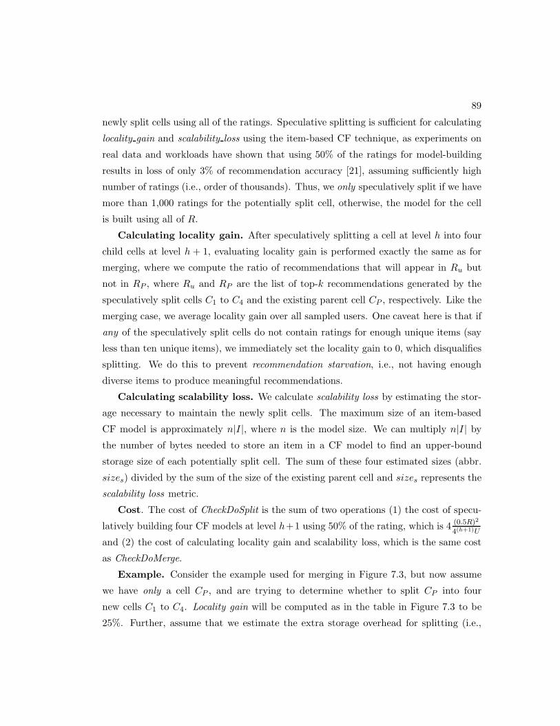
89

newly split cells using all of the ratings. Speculative splitting is sufficient for calculating

locality gain and scalability loss using the item-based CF technique, as experiments on

real data and workloads have shown that using 50% of the ratings for model-building

results in loss of only 3% of recommendation accuracy [21], assuming sufficiently high

number of ratings (i.e., order of thousands). Thus, we only speculatively split if we have

more than 1,000 ratings for the potentially split cell, otherwise, the model for the cell

is built using all of R.

Calculating locality gain. After speculatively splitting a cell at level h into four

child cells at level h + 1, evaluating locality gain is performed exactly the same as for

merging, where we compute the ratio of recommendations that will appear in Ru but

not in RP , where Ru and RP are the list of top-k recommendations generated by the

speculatively split cells C1 to C4 and the existing parent cell CP , respectively. Like the

merging case, we average locality gain over all sampled users. One caveat here is that if

any of the speculatively split cells do not contain ratings for enough unique items (say

less than ten unique items), we immediately set the locality gain to 0, which disqualifies

splitting. We do this to prevent recommendation starvation, i.e., not having enough

diverse items to produce meaningful recommendations.

Calculating scalability loss. We calculate scalability loss by estimating the stor-

age necessary to maintain the newly split cells. The maximum size of an item-based

CF model is approximately n|I|, where n is the model size. We can multiply n|I| by

the number of bytes needed to store an item in a CF model to find an upper-bound

storage size of each potentially split cell. The sum of these four estimated sizes (abbr.

sizes) divided by the sum of the size of the existing parent cell and sizes represents the

scalability loss metric.

Cost. The cost of CheckDoSplit is the sum of two operations (1) the cost of specu-

latively building four CF models at level h+1 using 50% of the rating, which is 4 (0.5R)2

4(h+1)U

and (2) the cost of calculating locality gain and scalability loss, which is the same cost

as CheckDoMerge.

Example. Consider the example used for merging in Figure 7.3, but now assume

we have only a cell CP , and are trying to determine whether to split CP into four

new cells C1 to C4. Locality gain will be computed as in the table in Figure 7.3 to be

25%. Further, assume that we estimate the extra storage overhead for splitting (i.e.,

90

storage loss) to be 50%. AssumingM=0.7, then (0.7 * 25) > (0.3 * 50), meaning that

LARS will decide to split CP into four cells as locality gain is significantly higher than

scalability loss.

7.3.4 Partial Merging and Splitting

So far, we have assumed cells are merged and split in complete quadrants. We now

relax this constraint by discussing the changes to LARS necessary to support partial

merging and splitting of pyramid cells.

Partial Merging

It may be beneficial to partially merge at a more granular level in order to sacrifice less

locality while still gaining scalability. For example, in Figure 7.3 we may only want to

merge cells C1 and C2 while leaving cells C3 and C4 intact, meaning three child cells

would be maintained under the example parent CP . To support partial merging, all

techniques described in Section 7.4.3 remain the same, with two exceptions: (1) The

resulting merged candidate cell (e.g., C1 merged with C2, abbreviated C12) plays the

role of the “parent” cell in evaluating locality loss; (2) When calculating storage gain,

we must subtract the size of the resulting merge candidate cell (e.g., C12) from the sum

of the sizes of cells that will merge (e.g., C1 and C2), since we no longer discard the

merged cells completely, i.e., the resulting merged cell now replaces the individual cells.

Partial merging involves extra overhead (compared to merging complete quadrants)

since we must build, from scratch, the CF model for the candidate merge result cell

(e.g., C12) in order to calculate locality loss. In order to perform the build efficiently,

we perform a speculative merge that builds the CF model using only 50% of the rating

data. This is the same method used in speculative splitting (Section 7.4.3), except

applied to the case of merging.

Partial Splitting

To support partial splitting, all techniques discussed in Section 7.4.3 remain the same.

There are, however, two distinguishable cases of partial splitting: (1) A “parent” at

level h splitting into less than four cells at level h + 1. This case requires speculative

91

splitting to be aware of which “partial” child cells to create. (2) A cell at level h is

split into two or three separate cells that remain at level h, i.e., cells at level h+ 1 are

not created. This case requires that a previous partial merge took place that originally

reduced a cell quadrant to two or three cells.

7.4 Optimized Spatial User Ratings for Non-Spatial Items

In this section, we present LARS*, an extension to LARS that employs a partial in-

memory pyramid structure [63] (equivalent to a partial quad-tree [64]) as depicted in

Figure 7.2. The pyramid decomposes the space into H levels (i.e., pyramid height). For

a given level h, the space is partitioned into 4h equal area grid cells. For example, at

the pyramid root (level 0), one grid cell represents the entire geographic area, level 1

partitions space into four equi-area cells, and so forth.

To provide a tradeoff between recommendation locality and system scalability, the

pyramid data structure maintains three types of cells (see figure 7.2): (1) Recommen-

dation Model Cell (α-Cell), (2) Statistics Cell (β-Cell), and (3) Empty Cell (γ-Cell),

explained as follows:

Recommendation Model Cell (α-Cell). Each α-Cell stores an item-based col-

laborative filtering model built using only the spatial ratings with user locations con-

tained in the cell’s spatial region. Note that the root cell (level 0) of the pyramid is an

α-Cell and represents a “traditional” (i.e., non-spatial) item-based collaborative filtering

model. Moreover, each α-Cell maintains statistics about all the ratings located within

the spatial extents of the cell. Each α-Cell Cp maintains a hash table that indexes all

items (by their IDs) that have been rated in this cell, named Items Ratings Statistics

Table. For each indexed item i in the Items Ratings Statistics Table, we maintain four

parameters; each parameter represent the number of user ratings to item i in each of the

four children cells (i.e., C1, C2, C3, and C4) of cell Cp. An example of the maintained

parameters is given in Figure 7.4. Assume that cell Cp contains ratings for three items

I1, I2, and I3. Figure 7.4 shows the maintained statistics for each item in cell Cp. For

example, for item I1, the number of user ratings located in child cell C1, C2, C3, and

C4 is equal to 109, 3200, 14, and 54, respectively. Similarly, the number of user ratings

is calculated for items I2 and I3.

92

!"#

$"#

$%#

$&#

$'#

"()#

&%((#

"'#

*'#

!%#

$"#

$%#

$&#

$'#

""("#

"*((#

)+,#

"&')#

!&#

$"#

$%#

$&#

$'#

*'#

*(*#

%&((#

"-(,#

./01#23456/#$7859# ./01#23456/#$7859# ./01#23456/#$7859#

Fig. 7.4: Example of Items Ratings Statistics Table

Level h -1

Level h

U1 U2

U3 U4

Cp U5

U6 U7

U8

U2 U1

U3

U4

C1

C3

C4

C2 U5

U6

U7

U8

Fig. 7.5: Two-Levels Pyramid

Statistics Cell (β-Cell). Like an α-Cell, a β-Cell maintains statistics (i.e., items

ratings Statistics Table) about the user/item ratings that are located within the spatial

range of the cell. The only difference between an α-Cell and a β-Cell is that a β-Cell

does not maintain a collaborative filtering (CF) model for the user/item ratings lying

in its boundaries. In consequence, a β-Cell is a light weight cell such that it incurs less

storage than an α-Cell. In favor of system scalability, LARS* prefers a β-Cell over an

α-Cell to reduce the total system storage.

Empty Cell (γ-Cell). a γ-Cell is a cell that maintains neither the statistics nor

the recommendation model for the ratings lying within its boundaries. a γ-Cell is the

most light weight cell among all cell types as it almost incurs no storage overhead. Note

that an α-Cell can have α-Cells, β-Cells, or γ-Cells children. Also, a β-Cell can have

α-Cells, β-Cells, or γ-Cells children. However, a γ-Cell cannot have any children.

7.4.1 Pyramid structure intuition

An α-Cell requires the highest storage and maintenance overhead because it maintains

a CF model as well as the user/item ratings statistics. On the other hand, an α-Cell

(as opposed to β-Cell and γ-Cell) is the only cell that can be leveraged to answer

93

!"#$%#&"#

!"#$%#&'#

!"#$%#&(#

!(#$%#&"#

!(#$%#&(#

C2

C4

C3

!)#$%#&)#

!)#$%#&*#

!*#$%#&'#

!*#$%#&*#

!*#$%#&+#

!'#$%#&'#

!'#$%#&,#

!'#$%#&+#

!,#$%#&)#

!,#$%#&*#

!'#$%#&,#

Cp

&-./0# 1-./"# 2345.#

!"# !$# %&'#

!"# !(# %&)#

!*# !)# %&)#

!*# !+# %&,#

!+# !)# %&+#

-# -# -#

Cp Model

&-./0# 1-./"# 2345.#

!,# !$# %&'#

!,# !+# %&+#

!,# !'# %&"#

-# -# -#

&-./0# 1-./"# 2345.#

!,# !+# %&(#

!,# !$# %&$#

!,# !'# %&,#

-# -# -#

C3 Model

C4 Model

&-./0# 1-./"# 2345.#

!*# !)# %&)#

!*# !+# %&,#

!+# !)# %&+#

C2 Model

C1

!0#$%#&0#

!0#$%#&,#

!*#$%#&0#

!*#$%#&*#

&-./0# 1-./"# 2345.#

!"# !$# %&'#

!"# !(# %&)#

-# -# -#

C1 Model

Fig. 7.6: Ratings Distribution and Recommendation Models

recommendation queries. A pyramid structure that only contains α-Cells achieves the

highest recommendation locality, and this is why an α-Cell is considered the highly

ranked cell type in LARS*. a β-Cell is the secondly ranked cell type as it only maintains

statistics about the user/item ratings. The storage and maintenance overhead incurred

by a β-Cell is less expensive than an α-Cell. The statistics maintained at a β-Cell

determines whether the children of that cell needs to be maintained as α-Cells to serve

more localized recommendation. Finally, a γ-Cell (lowest ranked cell type) has the least

maintenance cost, as neither a CF model nor statistics are maintained for that cell.

Moreover, a γ-Cell is a leaf cell in the pyramid.

LARS* upgrades (downgrades) a cell to a higher (lower) cell rank, based on trade-

offs between recommendation locality and system scalability (discussed in Section 7.3.3).

If recommendation locality is preferred over scalability, more α-Cells are maintained in

the pyramid. On the other hand, if scalability is favored over locality, more γ-Cells exist

in the pyramid. β-Cells comes as an intermediary stage between α-Cells and γ-Cells to

further increase the recommendation locality whereas the system scalability is not quite

affected.

94

!"#$% &'()*+&% &',)*+&% -.)*+%

!"# "# $# $%$#

!&# "# $# $%$#

!'# "# "# "%$#

!(# '# '# "%$#

!)# "# $# $%$#

!*# '# &# $%***#

!+# *# &# $%"**#

!,# "# "# "%$#

)#//%-012/+"3%.2+4%5-.)*+6% $%(,#

Fig. 7.7: Locality Loss/Gain at Cp]

We chose to employ a pyramid as it is a “space-partitioning” structure that is guar-

anteed to completely cover a given space. For our purposes, “data-partitioning” struc-

tures (e.g., R-trees) are less ideal than a “space-partitioning” structure for two main

reasons: (1) “data-partitioning” structures index data points, and hence covers only

locations that are inserted in them. In other words, “data-partitioning” structures are

not guaranteed to completely cover a given space, which is not suitable for queries

issued in arbitrary spatial locations. (2) In contrast to “data-partitioning” structures

(e.g., R-trees [66]), “space partitioning” structures show better performance for dynamic

memory resident data [67, 68, 65].

7.4.2 LARS* versus LARS

Table 7.1 compares LARS* against LARS. Like LARS*, LARS [69] employs a partial

pyramid data structure to support spatial user ratings for non-spatial items. LARS

is different from LARS* in the following aspects: (1) As shown in Table 7.1, LARS*

maintains α-Cells, β-Cells, and γ-Cells, whereas LARS only maintains α-Cells and γ-

Cells. In other words, LARS either merges or splits a pyramid cell based on a tradeoff

between scalability and recommendation locality. LARS* employs the same tradeoff

and further increases the recommendation locality by allowing for more α-Cells to be

maintained at lower pyramid levels. (2) As opposed to LARS, LARS* does not perform a

speculative splitting operation to decide whether to maintain more localized CF models.

However, LARS maintains extra statistics at each α-Cell and β-Cell that helps in quickly

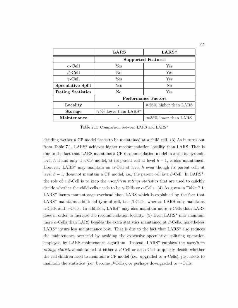
95

LARS LARS*

Supported Features

α-Cell Yes Yes

β-Cell No Yes

γ-Cell Yes Yes

Speculative Split Yes No

Rating Statistics No Yes

Performance Factors

Locality - ≈26% higher than LARS

Storage ≈5% lower than LARS* -

Maintenance - ≈38% lower than LARS

Table 7.1: Comparison between LARS and LARS*

deciding wether a CF model needs to be maintained at a child cell. (3) As it turns out

from Table 7.1, LARS* achieves higher recommendation locality than LARS. That is

due to the fact that LARS maintains a CF recommendation model in a cell at pyramid

level h if and only if a CF model, at its parent cell at level h − 1, is also maintained.

However, LARS* may maintain an α-Cell at level h even though its parent cell, at

level h − 1, does not maintain a CF model, i.e., the parent cell is a β-Cell. In LARS*,

the role of a β-Cell is to keep the user/item ratings statistics that are used to quickly

decide whether the child cells needs to be γ-Cells or α-Cells. (4) As given in Table 7.1,

LARS* incurs more storage overhead than LARS which is explained by the fact that

LARS* maintains additional type of cell, i.e., β-Cells, whereas LARS only maintains

α-Cells and γ-Cells. In addition, LARS* may also maintain more α-Cells than LARS

does in order to increase the recommendation locality. (5) Even LARS* may maintain

more α-Cells than LARS besides the extra statistics maintained at β-Cells, nonetheless

LARS* incurs less maintenance cost. That is due to the fact that LARS* also reduces

the maintenance overhead by avoiding the expensive speculative splitting operation

employed by LARS maintenance algorithm. Instead, LARS* employs the user/item

ratings statistics maintained at either a β-Cell or an α-Cell to quickly decide whether

the cell children need to maintain a CF model (i.e., upgraded to α-Cells), just needs to

maintain the statistics (i.e., become β-Cells), or perhaps downgraded to γ-Cells.

96

7.4.3 Pyramid Maintenance

This section describes building and maintaining the pyramid data structure. Initially,

to build the pyramid, all location-based ratings currently in the system are used to

build a complete pyramid of height H, such that all cells in all H levels are α-Cells and

contain ratings statistics and a collaborative filtering model. The initial height H is

chosen according to the level of locality desired, where the cells in the lowest pyramid

level represent the most localized regions. After this initial build, we invoke a cell type

maintenance step that scans all cells starting from the lowest level h and downgrades

cell types to either (β-Cell or γ-Cell) if necessary (cell type switching is discussed in

Section 7.4.3). We note that while the original partial pyramid [63] was concerned with

spatial queries over static data, it did not address pyramid maintenance.

Main idea. As time goes by, new users, ratings, and items will be added to the

system. This new data will both increase the size of the collaborative filtering mod-

els maintained in the pyramid cells, as well as alter recommendations produced from

each cell. To account for these changes, LARS* performs maintenance on a cell-by-cell

basis. Maintenance is triggered for a cell C once it receives N% new ratings; the per-

centage is computed from the number of existing ratings in C. We do this because an

appealing quality of collaborative filtering is that as a model matures (i.e., more data

is used to build the model), more updates are needed to significantly change the top-k

recommendations produced from it [17]. Thus, maintenance is needed less often.

We note the following features of pyramid maintenance: (1) Maintenance can be

performed completely offline, i.e., LARS* can continue to produce recommendations

using the ”old” pyramid cells while part of the pyramid is being updated; (2) mainte-

nance does not entail rebuilding the whole pyramid at once, instead, only one cell is

rebuilt at a time; (3) maintenance is performed only after N% new ratings are added

to a pyramid cell, meaning maintenance will be amortized over many operations.

Maintenance Algorithm. Algorithm 8 provides the pseudocode for the LARS*

maintenance algorithm. The algorithm takes as input a pyramid cell C and level h,

and includes three main steps: Statistics Maintenance, Model Rebuild and Cell Child

Quadrant Maintenance, explained below.

Step I: Statistics Maintenance. The first step (line 4) is to maintain the Items

Ratings Statistics Table. The maintained statistics are necessary for cell type switching

97

Algorithm 8 Pyramid maintenance algorithm

/* Called after cell C receives N% new ratings */Function PyramidMaintenance(Cell C, Level h)/* Step I: Statistics Maintenance*/Maintain cell C statistics/*Step II: Model Rebuild */if (Cell C is an α-Cell) then

Rebuild item-based collaborative filtering model for cell C/*Step III: Cell Child Quadrant Maintenance */if (C children quadrant q cells are α-Cells) then

CheckDownGradeToSCells(q,C) /* covered in Section 7.4.3 */else if (C children quadrant q cells are γ-Cells) then

CheckUpGradeToSCells(q,C)else

isSwitchedToMcells ← CheckUpGradeToMCells(q,C) /* covered in Section 7.4.3 */if (isSwitchedToMcells is False) then

CheckDownGradeToECells(q,C)return

decision, especially when new location-based ratings enter the system. As the items

ratings statistics table is implemented using a hash table, then it can be queried and

maintained in O(1)) time, requiring O(|IC |) space such that IC is the set of all items

rated at cell C and |IC | is the total number of items in IC .

Step II: Model Rebuild. The second step is to rebuild the item-based collabora-

tive filtering (CF) model for a cell C (line 7). The model is rebuilt at cell C only if cell C

is an α-Cell, otherwise (β-Cell or γ-Cell) no CF recommendation model is maintained,

and hence the model rebuild step does not apply Rebuilding the CF model is necessary

to allow the model to “evolve” as new location-based ratings enter the system (e.g.,

accounting for new items, ratings, or users).

Step III: Cell Child Quadrant Maintenance. LARS* invokes a maintenance

step that may decide whether cell C child quadrant need to be switched to a different

cell type based on trade-offs between scalability and locality. The algorithm first checks

if cell C child quadrant q at level h + 1 is of type α-Cell (line 9). If that case holds,

LARS* considers quadrant q cells as candidates to be downgraded to β-Cells (calling

function CheckDownGradeToSCells on line 10). We provide details of the Downgrade

α-Cells to β-Cells operation in Section 7.4.3. On the other hand, if C have a child

98

quadrant of type γ-Cells at level h + 1 (line 11), LARS* considers upgrading cell C

four children cells at level h + 1 to β-Cells (calling function CheckUpGradeToSCells

on line 12). The Updgrade From E to β-Cells operation is covered in Section 7.4.3.

However, if C have a child quadrant of type β-Cells at level h + 1 (line 11), LARS*

first considers upgrading cell C four children cells at level h + 1 from β-Cells to α-

Cells (calling function CheckUpGradeToMCells on line 14). If the children cells are

not switched to α-Cells, LARS* then considers downgrading them to γ-Cells (calling

function CheckDownGradeToECells on line 16). Cell Type switching operations are

performed completely in quadrants (i.e., four equi-area cells with the same parent). We

made this decision for simplicity in maintaining the partial pyramid.

Recommendation Locality

In this section, we explain the notion of locality in recommendation that is essential to

understand the cell type switching (upgrade/downgrade) operations highlighted in the

PyramidMaintenance algorithm (algorithm 8). We use the following example to give the

intuition behind recommendation locality.

Running Example. Figure 7.5 depicts a two-levels pyramid in which Cp is the root

cell and its children cells are C1, C2, C3, and C4. In the example, we assume eight users

(U1, U2, ..., and U8) have rated eight different items (I1, I2, ..., and I8). Figure 7.6 gives

the spatial distributions of users U1, U2, U3, U4, U5, U6, U7, and U8 as well as the items

that each user rated.

Intuition. Consider the example given in Figure 7.5. In cell Cp, users U2 and U5 that

belongs to the child cell C2 have both rated items I2 and I5. In that case, the similarity

score between items I2 and I5 in the item-based collaborative filtering CF model built

at cell C2 is exactly the same as the one in the CF model built at cell Cp. The last

phenomenon happened because items (i.e., I2 and I5) have been rated by mostly users

located in the same child cell, and hence the recommendation model at the parent cell

will not be different from the model at the children cells. In this case, if the CF model

at C2 is not maintained, LARS* does not lose recommendation locality at all.

The opposite case happens when an item is rated by users located in different pyra-

mid cells (spatially skewed). For example, item I4 is rated by users U2, U4, and U7

in three different cells (C2, C3, and C4). In this case, U2, U4, and U7 are spatially

99

Parameter Description

RPc,i The set of user pairs that co-rated item i in cell c

RSc,i The set of user pairs that co-rated item i in cell csuch that each pair of users 〈u1, u2〉 ∈ Sc,i are notlocated in the same child cell of c

LGc,i The degree of locality lost for item i from down-grading the four children of cell c to β-Cells, suchthat 0 ≤ LGc,i ≤ 1

LGc The amount of locality lost by downgrading cell cfour children cells to β-Cells (0 ≤ LGc ≤ 1)

Table 7.2: Summary of Mathematical Notations.

skewed. Hence, the similarity score between item I4 and other items at the children

cells is different from the similarity score calculated at the parent cell Cp because not

all users that have rated item I4 exist in the same child cell. Based on that, we observe

the following:

Observation 1 The more the user/item ratings in a parent cell C are geographically

skewed, the higher the locality gained from building the item-based CF model at the four

children cells.

The amount of locality gained/lost by maintaining the child cells of a given pyramid

cell depends on whether the CF models at the child cells are similar to the CF model

built at the parent cell. In other words, LARS* loses locality if the child cells are not

maintained even though the CF model at these cells produce different recommendations

than the CF model at the parent cell. LARS* leverages Observation 1 to determine the

amount of locality gained/lost due to maintaining an item-based CF model at the four

children. LARS* calculates the locality loss/gain as follows:

Locality Loss/Gain. Table 7.2 gives the main mathematical notions used in calculat-

ing the recommendation locality loss/gain. First, the Item Ratings Pairs Set (RPc,i) is

defined as the set of all possible pairs of users that rated item i in cell c. For example,

in figure 7.7 the item ratings pairs set for item I7 in cell Cp (RPCp,I7) has three elements

(i.e., RPCp,I7={〈U3, U6〉,〈U3, U7〉,〈U6, U7〉}) as only users U1 and U7 have rated item I1.

Similarly, RPCp,I2 is equal to {〈U6, U7〉} (i.e., Users U2 and U5 have rated item I2).

100

For each item, we define the Skewed Item Ratings Set (RSc,i) as the total number of

user pairs in cell c that rated item i such that each pair of users ∈ RSc,i do not exist in the

same child cell of c. For example, in Figure 7.7, the skewed item ratings set for item I2 in

cell Cp (RSCP ,I2) is ∅ as all users that rated I2, i.e., U2 and U5 are collocated in the same

child cell C2. For I4, the skewed item ratings set RSCP ,I2={〈U2, U7〉, 〈U2, U4〉, 〈U4, U7〉}

as all users that rated item I2 are located in different child cells,i.e., U2 at C2, U4 at C4,

and U7 at C3.

Given the aforementioned parameters, we calculate Item Locality Loss (LGc,i) for

each item, as follows:

Definition 1 Item Locality Loss (LGc,i)

LGc,i is defined as the degree of locality lost for item i from downgrading the four children

of cell c to β-Cells, such that 0 ≤ LGc,i ≤ 1.

LGc,i =|RSc,i|

|RPc,i|(7.3)

The value of both |RSc,i| and |RPc,i| can be easily extracted using the items ratings

statistics table. Then, we use the LGc,i values calculated for all items in cell c in order

to calculate the overall Cell Locality loss (LGc) from downgrading the children cells of

c to α-Cells.

Definition 2 Locality Loss (LGc)

LGc is defined as the total locality lost by downgrading cell c four children cells to β-

Cells (0 ≤ LGc ≤ 1). It is calculated as the the sum of all items locality loss normalized

by the total number of items |Ic| in cell c.

LGc =

∑

i∈Ic LGc,i

|Ic|(7.4)

The cell locality loss (or gain) is harnessed by LARS* to determine whether the cell

children need to be downgraded from α-Cell to β-Cell rank, upgraded from the γ-Cell to

β-Cell rank, or downgraded from β-Cell to γ-Cell rank. During the rest of section 7.3,

we explain the cell rank upgrade/downgrade operations.

Downgrade α-Cells to β-Cells

That operation entails downgrading an entire quadrant of cells from M-Cells to β-Cells

at level h with a common parent at level h−1. Downgrading α-Cells to β-Cells improves

101

scalability (i.e., storage and computational overhead) of LARS*, as it reduces storage

by discarding the item-based collaborative filtering (CF) models of the the four children

cells. Furthermore, downgrading α-Cells to β-Cells leads to the following performance

improvements: (a) less maintenance cost, since less CF models are periodically rebuilt,

and (b) less continuous query processing computation, as β-Cells does not maintain a CF

model and if many β-Cells cover a large spatial region, hence, for users crossing β-Cells

boundaries, we do not need to update the recommendation query answer. Downgrading

children cells from α-Cells to β-Cells might hurt recommendation locality, since no CF

models are maintained at the granularity of the child cells anymore.

At cell Cp, in order to determine whether to downgrade a quadrant q cells to β-

Cells (i.e., function CheckDownGradeToSCells on line 10 in Algorithm 8), we calculate

two percentage values: (1) locality loss (see equation 7.4), the amount of locality lost

by (potentially) downgrading the children cells to β-Cells, and (2) scalability gain, the

amount of scalability gained by (potentially) downgrading the children cells to β-Cells.

Details of calculating these percentages are covered next. When deciding to downgrade

cells to β-Cells, we define a system parameter M, a real number in the range [0,1]

that defines a tradeoff between scalability gain and locality loss. LARS* downgrades a

quadrant q cells to β-Cells (i.e., discards quadrant q) if Equation 7.1 holds true:

A smaller M value implies gaining scalability is important and the system is willing

to lose a large amount of locality for small gains in scalability. Conversely, a larger

M value implies scalability is not a concern, and the amount of locality lost must be

small in order to allow for β-Cells downgrade. At the extremes, setting M=0 (i.e.,

always switch to β-Cell) implies LARS* will function as a traditional CF recommender

system, while settingM=1 causes LARS* pyramid cells to all be α-Cells, i.e., LARS*

will employ a complete pyramid structure maintaining a recommendation model at all

cells at all levels.

Calculating Locality Loss. To calculate the locality loss at a cell Cp, LARS*

leverages the Item Ratings Statistics Table maintained in that cell. First, LARS* cal-

culates the item locality loss LGCp,i for each item i in the cell Cp. Therefore, LARS*

aggregates the item locality loss values calculated for each item i ∈ Cp, to finally deduce

the global cell locality loss LGCp .

102

Calculating scalability gain. Scalability gain is measured in storage and com-

putation savings. We measure scalability gain by summing the recommendation model

sizes for each of the downgraded (i.e., child) cells (abbr. sizem), and divide this value

by the sum of sizem and the recommendation model size of the parent cell. We refer to

this percentage as the storage gain. We also quantify computation savings using storage

gain as a surrogate measurement, as computation is considered a direct function of the

amount of data in the system.

Cost. using the Items Ratings Statistics Table maintained at cell Cp, the locality

loss at cell Cp can be calculated in O(|ICp |) time such that |ICp | represents the total

number of items in Cp. As scalability gain can be calculated in O(1) time, then the

total time cost of the Downgrade To β-Cells operation is O(|ICp |).

Example. For the example given in Figure 7.7, the locality loss of downgrading

cell Cp four children cells {C1, C2, C3, C4} to β-Cells is calculated as follows: First,

we retrieve the locality loss LGCp,i for each item i ∈ {I1, I2, I3, I4, I5, I6, I7, I8}, from

the maintained statistics at cell Cp. As given in figure 7.7, LGCp,I1 , LGCp,I2 , LGCp,I3 ,

LGCp,I4 , LGCp,I5 , LGCp,I6 , LGCp,I7 , and LGCp,I8 are equal to 0.0, 0.0, 1.0, 1.0, 0.0,

0.666, 0.166, and 1.0, respectively. Then, we calculate the overall locality loss at Cp

(using equation 7.4), LGCp by summing all the locality loss values of all items and

dividing the sum by the total number of items. Hence, the scalability loss is equal to

(0.0+0.0+1.0+1.0+0.0+1.0+0.666+1.08 ) = 0.48 = 48%. To calculate scalability gain, assume

the sum of the model sizes for cells C1 to C4 and CP is 4GB, and the sum of the model

sizes for cells C1 to C4 is 2GB. Then, the scalability gain is 24=50%. AssumingM=0.7,

then (0.3 × 50) < (0.7 × 48), meaning that LARS* will not downgrade cells C1, C2,

C3, C4 to β-Cells.

Upgrade β-Cells to α-Cells

Upgrading β-Cells to α-Cells operation entails upgrading the cell type of a cell child

quadrant at pyramid level h under a cell at level h− 1, to α-Cells. Upgrading β-Cells to

α-Cells operation improves locality in LARS*, as it leads to maintaining a CF model

at the children cells that represent more granular spatial regions capable of producing

recommendations unique to the smaller, more “local”, spatial regions. On the other

hand, upgrading cells to α-Cells hurts scalability by requiring storage and maintenance

103

of more item-based collaborative filtering models. The upgrade to α-Cells operation

also negatively affects continuous query processing, since it creates more granular α-Cells

causing user locations to cross α-Cell boundaries more often, triggering recommendation

updates.

To determine whether to upgrade a cell CP (quadrant q) four children cells to α-Cells

(i.e., function CheckUpGradeToMCells on line 14 of Algorithm 8). Two percentages are

calculated: locality gain and scalability loss. These values are the opposite of those

calculated for the Upgrade to β-Cells operation. LARS* change cell CP child quadrant

q to α-Cells only if the condition in Equation 7.2 holds.

This equation represents the opposite criteria of that presented for Upgrade to β-Cells

operation in Equation 7.1.

Calculating locality gain. To calculate the locality gain, LARS* does not need

to speculatively build the CF model at the four children cells. The locality gain is

calculated the same way the locality loss is calculated in equation 7.4.

Calculating scalability loss. We calculate scalability loss the same way we cal-

culated scalability gain in Section 7.4.3

Cost. Similar to the CheckDownGradeToSCells operation, scalability loss is calcu-

late in O(1) and locality gain can be calculated in O(|ICp |) time. Then, the total time

cost of the CheckUpGradeToMCells operation is O(|ICp |).

Example. Consider the example given in Figure 7.7. Assume the cell Cp is an

α-Cell and its four children C1, C2, C3, and C4 are β-Cells. The locality gain (LGCp)

is calculated using equation 7.4 to be 0.48 (i.e., 48%) as depicted in the table in Fig-

ure 7.7. Further, assume that we estimate the extra storage overhead for upgradinging

the children cells to α-Cells (i.e., storage loss) to be 50%. Assuming M=0.7, then

(0.7 × 48) > (0.3 × 50), meaning that LARS* will decide to upgrade CP four children

cells to α-Cells as locality gain is significantly higher than scalability loss.

Downgrade β-Cells to γ-Cells and Vice Versa

Downgrading β-Cells to γ-Cells operation entails downgrading the cell type of a cell child

quadrant at pyramid level h under a cell at level h − 1, to γ-Cells (i.e., empty cells).

Downgrading the child quadrant type to γ-Cells means that the maintained statistics

are no more maintained in the children cell, which definitely reduces the overhead of

104

maintaining the Item Ratings Statistics Table at these cells. Even though γ-Cells incurs

no maintenance overhead, however they reduce the amount of recommendation locality

that LARS* provides.

The decision of downgrading from β-Cells to γ-Cells is taken based on a system

parameter, namedMAX SLEVELS. It is defined as the maximum number of consecutive

pyramid levels in which descendant cells can be β-Cells. MAX SLEVELS can take any

value between zero and the total height of the pyramid. A high value of MAX SLEVELS

results in maintaining more β-Cells and less γ-Cells in the pyramid. For example, in

Figure 7.2, MAX SLEVELS is set to two, and this is why if two consecutive pyramid

levels are β-Cells, the third level β-Cells are autotmatically downgraded to γ-Cells. For

each β-Cell C, a counter, called S-Levels Counter, is maintained. The S-Levels Counter

stores of the total number of consecutive levels in the direct ancestry of cell C such that

all these levels contains β-Cells.

At a β-Cell C, if the cell children are β-Cells, then we compare the S-Levels Counter

at the child cells with the MAX SLEVELS parameter. Note that the counter counts

only the consecutive S-Levels, so if some levels in the chain are α-Cells the counter

is reset to zero at the α-Cells levels. If S-Levels Counter is greater than or equal to

MAX SLEVELS, then the children cells of C are downgraded to γ-Cells. Otherwise,

cell C children cells are not downgraded to γ-Cells. Similarly, LARS* also makes use of

the same S-Levels Counter to decide whether to upgrade γ-Cells to β-Cells.

7.5 Non-Spatial User Ratings for Spatial Items

This section describes how LARS produces recommendations using non-spatial ratings

for spatial items represented by the tuple (user, rating, item, ilocation). The idea is

to exploit travel locality, i.e., the observation that users limit their choice of spatial

venues based on travel distance (based on analysis in Section 7.1). Traditional (non-

spatial) recommendation techniques may produces recommendations with burdensome

travel distances (e.g., hundreds of miles away). LARS produces recommendations within

reasonable travel distances by using travel penalty, a technique that penalizes the rec-

ommendation rank of items the further in travel distance they are from a querying

user. Travel penalty may incur expensive computational overhead by calculating travel

105

distance to each item. Thus, LARS employs an efficient query processing technique

capable of early termination to produce the recommendations without calculating the

travel distance to all items. Section 7.5.1 describes the query processing framework

while Section 7.5.2 describes travel distance computation.

7.5.1 Query Processing

Query processing for spatial items using the travel penalty technique employs a single

system-wide item-based collaborative filtering model to generate the top-k recommen-

dations by ranking each spatial item i for a querying user u based on RecScore(u, i),

computed as:

RecScore(u, i) = P (u, i) − TravelPenalty(u, i) (7.5)

P (u, i) is the standard item-based CF predicted rating of item i for user u.

TravelPenalty(u, i) is the road network travel distance between u and i normalized

to the same value range as the rating scale (e.g., [0, 5]).

When processing recommendations, we aim to avoid calculating Equation 7.5 for all

candidate items to find the top-k recommendations, which can become quite expensive

given the need to compute travel distances. To avoid such computation, we evaluate

items in monotonically increasing order of travel penalty (i.e., travel distance), enabling

us to use early termination principles from top-k query processing [70, 71, 72]. We now

present the main idea of our query processing algorithm and in the next section discuss

how to compute travel penalties in an increasing order of travel distance.

Algorithm 9 provides the pseudo code of our query processing algorithm that takes

a querying user id U , a location L, and a limit K as input, and returns the list R

of top-k recommended items. The algorithm starts by running a k-nearest-neighbor

algorithm to populate the list R with k items with lowest travel penalty; R is sorted by

the recommendation score computed using Equation 7.5. This initial part is concluded

by setting the lowest recommendation score value (LowestRecScore) as the RecScore

of the kth item in R (Lines 3 to 7). Then, the algorithm starts to retrieve items one

by one in the order of their penalty score. This can be done using an incremental k-

nearest-neighbor algorithm, as will be described in the next section. For each item i, we

calculate the maximum possible recommendation score that i can have by subtracting

106

Algorithm 9 Travel Penalty Algorithm for Spatial Items

Function LARS SpatialItems(User U , Location L, Limit K)/* Populate a list R with a set of K items*/R ← φfor (K iterations) do

i ← Retrieve the item with the next lowest travel penalty (Section 7.5.2)Insert i into R ordered by RecScore(U, i) computed by Equation 7.5

LowestRecScore ← RecScore of the kth object in R/*Retrieve items one by one in order of their penalty value */while there are more items to process do

i ← Retrieve the next item in order of penalty score (Section 7.5.2)MaxPossibleScore ← MAX RATING - i.penaltyif MaxPossibleScore ≤ LowestRecScore then

return R /* early termination - end query processing */RecScore(U, i) ← P (U, i) - i.penalty /* Equation 7.5 */if RecScore(U, i) > LowestRecScore then

Insert i into R ordered by RecScore(U, i)LowestRecScore ← RecScore of the kth object in R

return R

the travel penalty of i from MAX RATING, the maximum possible rating value in the

system, e.g., 5 (Line 11). If i cannot make it into the list of top-k recommended items

with this maximum possible score, we immediately terminate the algorithm by returning

R as the top-k recommendations without computing the recommendation score (and

travel distance) for more items (Lines 12 to 13). The rationale here is that since we

are retrieving items in increasing order of their penalty and calculating the maximum

score that any remaining item can have, then there is no chance that any unprocessed

item can beat the lowest recommendation score in R. If the early termination case does

not arise, we continue to compute the score for each item i using Equation 7.5, insert

i into R sorted by its score (removing the kth item if necessary), and adjust the lowest

recommendation value accordingly (Lines 14 to 17).

Travel penalty requires very little maintenance. The only maintenance necessary is

to occasionally rebuild the single system-wide item-based collaborative filtering model

in order to account for new location-based ratings that enter the system. Following

the reasoning discussed in Section 7.3.3, we rebuild the model after receiving N% new

location-based ratings.

107

7.5.2 Incremental Travel Penalty Computation

This section gives an overview of two methods we implemented in LARS to incrementally

retrieve items one by one ordered by their travel penalty. The two methods exhibit

a trade-off between query processing efficiency and penalty accuracy: (1) an online

method that provides exact travel penalties but is expensive to compute, and (2) an

offline heuristic method that is less exact but efficient in penalty retrieval. Both methods

can be employed interchangeably in Line 10 of Algorithm 9.

Incremental KNN: An Exact Online Method

To calculate an exact travel penalty for a user u to item i, we employ an incremental

k-nearest-neighbor (KNN) technique [73, 74, 75]. Given a user location l, incremental

KNN algorithms return, on each invocation, the next item i nearest to u with regard

to travel distance d. In our case, we normalize distance d to the ratings scale to get the

travel penalty in Equation 7.5. Incremental KNN techniques exist for both Euclidean

distance [74] and (road) network distance [73, 75]. The advantage of using Incremental

KNN techniques is that they provide an exact travel distances between a querying user’s

location and each recommendation candidate item. The disadvantage is that distances

must be computed online at query runtime, which can be expensive. For instance,

the runtime complexity of retrieving a single item using incremental KNN in Euclidean

space is [74]: O(k + logN), where N and k are the number of total items and items

retrieved so far, respectively.

Penalty Grid: A Heuristic Offline Method

A more efficient, yet less accurate method to retrieve travel penalties incrementally is to

use a pre-computed penalty grid. The idea is to partition space using an n×n grid. Each

grid cell c is of equal size and contains all items whose location falls within the spatial

region defined by c. Each cell c contains a penalty list that stores the pre-computed

penalty values for traveling from anywhere within c to all other n2− 1 destination cells

in the grid; this means all items within a destination grid cell share the same penalty

value. The penalty list for c is sorted by penalty value and always stores c (itself) as

the first item with a penalty of zero. To retrieve items incrementally, all items within

108

the cell containing the querying user are returned one-by-one (in any order) since they

have no penalty. After these items are exhausted, items contained in the next cell in the

penalty list are returned, and so forth until Algorithm 9 terminates early or processes

all items.

To populate the penalty grid, we must calculate the penalty value for traveling from

each cell to every other cell in the grid. We assume items and users are constrained

to a road network, however, we can also use Euclidean space without consequence. To

calculate the penalty from a single source cell c to a destination cell d, we first find

the average distance to travel from anywhere within c to all item destinations within

d. To do this, we generate an anchor point p within c that both (1) lies on the road

network segment within c and (2) lies as close as possible to the center of c. With

these criteria, p serves as an approximate average “starting point” for traveling from c

to d. We then calculate the shortest path distance from p to all items contained in d

on the road network (any shortest path algorithm can be used). Finally, we average all

calculated shortest path distances from c to d. As a final step, we normalize the average

distance from c to d to fall within the rating value range. Normalization is necessary

as the rating domain is usually small (e.g., zero to five), while distance is measured in

miles or kilometers and can have large values that heavily influence Equation 7.5. We

repeat this entire process for each cell to all other cells to populate the entire penalty

grid.

When new items are added to the system, their presence in a cell d can alter the

average distance value used in penalty calculation for each source cell c. Thus, we

recalculate penalty scores in the penalty grid after N new items enter the system. We

assume spatial items are relatively static, e.g., restaurants do not change location often.

Thus, it is unlikely existing items will change cell locations and in turn alter penalty

scores.

7.6 Spatial User Ratings for Spatial Items

This section describes how LARS produces recommendations using spatial ratings for

spatial items represented by the tuple (user, ulocation, rating, item, ilocation). A salient

feature of LARS is that both the user partitioning and travel penalty techniques can be

109

used together with very little change to produce recommendations using spatial user

ratings for spatial items. The data structures and maintenance techniques remain ex-

actly the same as discussed in Sections 7.3 and 7.5; only the query processing framework

requires a slight modification. Query processing uses Algorithm 9 to produce recom-

mendations. However, the only difference is that the item-based collaborative filtering

prediction score P (u, i) used in the recommendation score calculation (Line 14 in Algo-

rithm 9) is generated using the (localized) collaborative filtering model from the partial

pyramid cell that contains the querying user, instead of the system-wide collaborative

filtering model as was used in Section 7.5.


This section provides experimental evaluation of LARS* based on an actual system

implementation using C++ and STL. We compare LARS* with the standard item-

based collaborative filtering technique along with several variations of LARS*. We also

compare LARS* to LARS [69]. Experiments are based on three data sets:

Foursquare: a real data set consisting of spatial user ratings for spatial items derived

from Foursquare user histories. We crawled Foursquare and collected data for 1,010,192

users and 642,990 venues across the United States. Foursquare does not publish each

“check-in” for a user, however, we were able to collect the following pieces of data:

(1) user tips for a venue, (2) the venues for which the user is the mayor, and (3) the

completed to-do list items for a user. In addition, we extracted each user’s friend list.

Extracting location-based ratings. To extract spatial user ratings for spatial items

from the Foursquare data (i.e., the five-tuple (user, ulocation, rating, item, ilocation)),

we map each user visit to a single location-based rating. The user and item attributes

are represented by the unique Foursquare user and venue identifier, respectively. We

employ the user’s home city in Foursquare as the ulocation attribute. Meanwhile, the

ilocation attribute is the item’s inherent location. We use a numeric rating value range

of [1, 3], translated as follows: (a) 3 represents the user is the “mayor” of the venue,

(b) 2 represents that the user left a “tip” at the venue, and (c) 1 represents the user

visited the venue as a completed “to-do” list item. Using this scheme, a user may have

multiple ratings for a venue, in this case we use the highest rating value.

110

Data properties. Our experimental data consisted of 22,390 location-based ratings

for 4K users for 2K venues all from the state of Minnesota, USA. We used this reduced

data set in order to focus our quality experiments on a dense rating sample. Use of

dense ratings data has been shown to be a very important factor when testing and

comparing recommendation quality [17], since use of sparse data (i.e., having users or

items with very few ratings) tends to cause inaccuracies in recommendation techniques.

MovieLens: a real data set consisting of spatial user ratings for non-spatial items taken

from the popular MovieLens recommender system [50]. The Foursquare and MovieLens

data are used to test recommendation quality. The MovieLens data used in our exper-

iments was real movie rating data taken from the popular MovieLens recommendation

system at the University of Minnesota [50]. This data consisted of 87,025 ratings for

1,668 movies from 814 users. Each rating was associated with the zip code of the user

who rated the movie, thus giving us a real data set of spatial user ratings for non-spatial

items.

Synthetic: a synthetically generated data set consisting of spatial user ratings for

spatial items for venues in the state of Minnesota, USA. The synthetic data set we

use in our experiments is generated to contain 2000 users and 1000 items, and 500,000

ratings. Users and items locations are randomly generated over the state of Minnesota,

USA. Users’ ratings to items are assigned random values between zero and five. As this

data set contains a number of ratings that is about twenty five times and five times

larger than the foursquare data set and the Movielens data set, we use such synthetic

data set to test scalability and query efficiency.

Unless mentioned otherwise, the default value of M is 0.3, k is 10, the number of

pyramid levels is 8, the influence level is the lowest pyramid level, and MAX SLEVELS

is set to two. The rest of this section evaluates LARS* recommendation quality (Sec-

tion 7.7.1), trade-offs between storage and locality (Section 7.7.4), scalability (Sec-

tion 7.7.5), and query processing efficiency (Section 7.7.6). As the system stores its

data structures in main memory, all reported time measurements represent the CPU

time.

111

1.4x

1.6x

1.8x

2x

1 2 3 4 5 6 7 8

Qua

lity

Impr

ovem

ent

Pyramid Level

LARS*LARS*−ULARS−T

0.6x

0.8x

1x

1.2x

(a) Foursquare data

1 2 3 4 5 6 7 8

Qua

lity

Impr

ovem

ent

Pyramid Level

LARS*−ULARS*

5x

10x

15x

20x

25x

(b) MovieLens data

Fig. 7.8: Quality experiments for varying locality

7.7.1 Recommendation Quality for Varying Pyramid Levels

These experiments test the recommendation quality improvement that LARS* achieves

over the standard (non-spatial) item-based collaborative filtering method using both the

Foursquare and MovieLens data. To test the effectiveness of our proposed techniques, we

test the quality improvement of LARS* with only travel penalty enabled (abbr. LARS*-

T), LARS* with only user partitioning enabled and M set to one (abbr. LARS*-U), and

LARS* with both techniques enabled and M set to one (abbr. LARS*). Notice that

LARS*-T represents the traditional item-based collaborative filtering augmented with

the travel penalty technique (section 7.5) to take the distance between the querying

user and the recommended items into account. We do not plot LARS with LARS* as

both give the same result for M=1, and the quality experiments are meant to show how

locality increases the recommendation quality.

Quality Metric. To measure quality, we build each recommendation method using

80% of the ratings from each data set. Each rating in the withheld 20% represents a

Foursquare venue or MovieLens movie a user is known to like (i.e., rated highly). For

each rating t in this 20%, we request a set of k ranked recommendations S by submitting

the user and ulocation associated with t. We first calculate the quality as the weighted

sum of the number of occurrences of the item associated with t (the higher the better)

in S. The weight of an item is a value between zero and one that determines how close

the rank of this item from its real rank. The quality of each recommendation method is

calculated and compared against the baseline, i.e., traditional item-based collaborative

112

filtering. We finally report the ratio of improvement in quality each recommendation

method achieves over the baseline. The rationale for this metric is that since each with-

held rating represents a real visit to a venue (or movie a user liked), the technique that

produces a large number of correctly ranked answers that contain venues (or movies) a

user is known to like is considered of higher quality.

Figure 7.8(a) compares the quality improvement of each technique (over traditional

collaborative filtering) for varying locality (i.e., different levels of the adaptive pyra-

mid) using the Foursquare data. LARS*-T does not use the adaptive pyramid, thus

has constant quality improvement. However, LARS*-T shows some quality improve-

ment over traditional collaborative filtering. This quality boost is due to that fact

that LARS*-T uses a travel penalty technique that recommends items within a feasible

distance. Meanwhile, the quality of LARS* and LARS*-U increases as more localized

pyramid cells are used to produce recommendation, which verifies that user partitioning

is indeed beneficial and necessary for location-based ratings. Ultimately, LARS* has

superior performance due to the additional use of travel penalty. While travel penalty

produces moderate quality gain, it also enables more efficient query processing, which

we observe later in Section 7.7.6.

Figure 7.8(b) compares the quality improvement of LARS*-U over CF (traditional

collaborative filtering) for varying locality using the MovieLens data. Notice that

LARS* gives the same quality improvement as LARS*-U because LARS*-T do not apply

for this dataset since movies are not spatial. Compared to CF, the quality improvement

achieved by LARS*-U (and LARS*) increases when it produces movie recommendations

from more localized pyramid cells. This behavior further verifies that user partitioning

is beneficial in providing quality recommendations localized to a querying user location,

even when items are not spatial. Quality decreases (or levels off for MovieLens) for

both LARS*-U and/or LARS* for lower levels of the adaptive pyramid. This is due

to recommendation starvation, i.e., not having enough ratings to produce meaningful

recommendations.

7.7.2 Recommendation Quality for Varying k

These experiments test recommendation quality improvement of LARS*, LARS*-U, and

LARS*-T for different values of k (i.e., recommendation answer sizes). We do not plot

113

0.6x

0.8x

1x

1.2x

1.4x

1.6x

1.8x

2x

1 3 5 10

Qua

lity

Impr

ovem

ent

Number of Recommended Items (K)

LARS*LARS*−ULARS−T

(a) Foursquare data

10x

15x

20x

25x

1 3 5 10

Qua

lity

Impr

ovem

ent

Number Of Recommended Items (K)

LARS*−ULARS*

5x

(b) MovieLens data

Fig. 7.9: Quality experiments for varying answer sizes

LARS with LARS* as both gives the same result for M=1, and the quality experiments

are meant to show how the degree of locality increases the recommendation quality.

We perform experiments using both the Foursquare and MovieLens data. Our quality

metric is exactly the same as presented previously in Section 7.7.1.

Figure 7.9(a) depicts the effect of the recommendation list size k on the quality of

each technique using the Foursquare data set. We report quality numbers using the

pyramid height of four (i.e., the level exhibiting the best quality from Section 7.7.1 in

Figure 7.8(a)). For all sizes of k from one to ten, LARS* and LARS*-U consistently

exhibit better quality. In fact, LARS* consistently achieves better quality over CF for

all k. LARS*-T exhibits similar quality to CF for smaller k values, but does better for

k values of three and larger.

Figure 7.9(b) depicts the effect of the recommendation list size k on the quality of

improvement of LARS*-U (and LARS*) over CF using the MovieLens data. Notice

that LARS* gives the same quality improvement as LARS*-U because LARS*-T do

not apply for this dataset since movies are not spatial. This experiment was run using

a pyramid hight of seven (i.e., the level exhibiting the best quality in Figure 7.8(b)).

Again, LARS*-U (and LARS*) consistently exhibits better quality than CF for sizes of

K from one to ten.

114

1.1

1.2

1.3

1.4

1.5

1.6

1.7

1.8

1.9

2

0 0.1 0.2 0.3 0.4 0.5 0.6 0.7 0.8 0.9 1

Qu

ality

Im

pro

vem

en

t

M

LARS

LARS*

(a) Foursquare data

0

5

10

15

20

25

0 0.1 0.2 0.3 0.4 0.5 0.6 0.7 0.8 0.9 1

Qu

ality

Im

pro

vem

en

t

M

LARS

LARS*

(b) MovieLens data

Fig. 7.10: Quality experiments for varying value ofM

7.7.3 Recommendation Quality for Varying M

These experiments compares the quality improvement achieved by both LARS and

LARS* for different values ofM. We perform experiments using both the Foursquare

and MovieLens data. Our quality metric is exactly the same as presented previously in

Section 7.7.1.

Figure 7.10(a) depicts the effect of M on the quality of both LARS and LARS*

using the Foursquare data set. Notice that we enable both the user partitioning and

travel penalty techniques for both LARS and LARS*. We report quality numbers using

the pyramid height of four and the number of recommended items of ten. When M

is equal to zero, both LARS and LARS* exhibit the same quality improvement as

M = 0 represents a traditional collaborative filtering with the travel penalty technique

applied. Also, whenM is set to one, both LARS and LARS* achieve the same quality

improvement as a fully maintained pyramid is maintained in both cases. ForM values

between zero and one, the quality improvement of both LARS and LARS* increases for

higher values of M due to the increase in recommendation locality. LARS* achieves

better quality improvement over LARS because LARS* maintains α-Cells at lower levels

of the pyramid.

Figure 7.10(b) depicts the effect ofM on the quality of both LARS and LARS* using

the Movilens data set. We report quality improvement over traditional collaborative

filtering using the pyramid height of seven and the number of recommended items set to

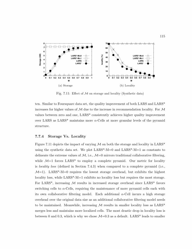
115

0

1

2

3

4

5

6

7

8

0 0.1 0.2 0.3 0.4 0.5 0.6 0.7 0.8 0.9 1

Sto

rag

e (

GB

)

M

LARS*-M=0

LARS*-M=1

LARS

LARS*

(a) Storage

0

10

20

30

40

50

60

70

0 0.1 0.2 0.3 0.4 0.5 0.6 0.7 0.8 0.9 1

locality

(%

)

M

LARS*-M=0

LARS*-M=1

LARS

LARS*

(b) Locality

Fig. 7.11: Effect ofM on storage and locality (Synthetic data)

ten. Similar to Foursquare data set, the quality improvement of both LARS and LARS*

increases for higher values ofM due to the increase in recommendation locality. ForM

values between zero and one, LARS* consistently achieves higher quality improvement

over LARS as LARS* maintains more α-Cells at more granular levels of the pyramid

structure.

7.7.4 Storage Vs. Locality

Figure 7.11 depicts the impact of varyingM on both the storage and locality in LARS*

using the synthetic data set. We plot LARS*-M=0 and LARS*-M=1 as constants to

delineate the extreme values ofM, i.e.,M=0 mirrors traditional collaborative filtering,

while M=1 forces LARS* to employ a complete pyramid. Our metric for locality

is locality loss (defined in Section 7.4.3) when compared to a complete pyramid (i.e.,

M=1). LARS*-M=0 requires the lowest storage overhead, but exhibits the highest

locality loss, while LARS*-M=1 exhibits no locality loss but requires the most storage.

For LARS*, increasing M results in increased storage overhead since LARS* favors

switching cells to α-Cells, requiring the maintenance of more pyramid cells each with

its own collaborative filtering model. Each additional α-Cell incurs a high storage

overhead over the original data size as an additional collaborative filtering model needs

to be maintained. Meanwhile, increasing M results in smaller locality loss as LARS*

merges less and maintains more localized cells. The most drastic drop in locality loss is

between 0 and 0.3, which is why we choseM=0.3 as a default. LARS* leads to smaller

116

locality loss (≈26% less) than LARS because LARS* maintains α-Cells below β-Cells

which result in higher locality gain. On the other hand, LARS* exhibits slightly higher

storage cost (≈5% more storage) than LARS due to the fact that LARS* stores the

Item Ratings Statistics Table per each α-Cell and β-Cell.

7.7.5 Scalability

Figure 7.12 depicts the storage and aggregate maintenance overhead required for an

increasing number of ratings using the synthetic data set. We again plot LARS*-M=0

and LARS*-M=1 to indicate the extreme cases for LARS*. Figure 7.12(a) depicts the

impact of increasing the number of ratings from 10K to 500K on storage overhead.

LARS*-M=0 requires the lowest amount of storage since it only maintains a single col-

laborative filtering model. LARS*-M=1 requires the highest amount of storage since it

requires storage of a collaborative filtering model for all cells (in all levels) of a complete

pyramid. The storage requirement of LARS* is in between the two extremes since it

merges cells to save storage. Figure 7.12(b) depicts the cumulative computational over-

head necessary to maintain the adaptive pyramid initially populated with 100K ratings,

then updated with 200K ratings (increments of 50K reported). The trend is similar to

the storage experiment, where LARS* exhibits better performance than LARS*-M=1

due to switching some cells from α-Cells to β-Cells. Though LARS*-M=0 has the best

performance in terms of maintenance and storage overhead, previous experiments show

that it has unacceptable drawbacks in quality/locality. Compare to LARS, LARS* has

less maintenance overhead (≈38% less) due to the fact that the maintenance algorithm

in LARS* avoids the expensive speculative splitting used by LARS.

7.7.6 Query Processing Performance

Figure 7.13 depicts snapshot and continuous query processing performance of LARS,

LARS*, LARS*-U (LARS* with only user partitioning), LARS*-T (LARS* with only

travel penalty), CF (traditional collaborative filtering), and LARS*-M=1 (LARS* with

a complete pyramid), using the synthetic data set.

Snapshot queries. Figure 7.13(a) gives the effect of various number of ratings (10K

to 500K) on the average snapshot query performance averaged over 500 queries posed

117

0

1

2

3

4

5

6

7

8

10 50 100 200 500

Sto

rag

e (

GB

)

Number of Ratings (* 1K)

LARS*-M=0

LARS*-M=1

LARS

LARS*

(a) Storage

0

2

4

6

8

10

12

14

16

18

10 50 100 150 200

Ag

gre

gate

Main

t T

ime (

* 1K

sec)

Number of Ratings So Far (* 1K)

LARS*-M=0

LARS*-M=1

LARS

LARS*

(b) Maintenance

Fig. 7.12: Scalability of the adaptive pyramid (Synthetic data)

20

40

60

80

100

120

10 50 100 200 500

Resp

on

se T

ime (

ms)

Number of Ratings (* 1K)

LARS*-M=0

LARS*-M=1

LARS

LARS*

LARS*-T

LARS*-U

(a) Snapshot Queries

0

0.2

0.4

0.6

0.8

1

1.2

1.4

1.6

1.8

0.6 3 6.2 9.3 12.4 15.5 18.6

Ag

gre

gate

Resp

on

se T

ime (

sec)

Travel Distance (miles)

LARS*-M=0

LARS*-M=1

LARS

LARS*

LARS*-T

LARS*-U

(b) Continuous Queries

Fig. 7.13: Query Processing Performance (Synthetic data).

at random locations. LARS* and LARS*-M=1 consistently outperform all other tech-

niques; LARS*-M=1 is slightly better due to recommendations always being produced

from the smallest (i.e., most localized) CF models. The performance gap between

LARS* and LARS*-U (and CF and LARS*-T) shows that employing the travel penalty

technique with early termination leads to better query response time. Similarly, the

performance gap between LARS* and LARS*-T shows that employing user partition-

ing technique with its localized (i.e., smaller) collaborative filtering model also benefits

query processing. LARS* performance is slightly better than LARS as LARS* some-

times maintains more localized CF models than LARS which incurs less query processing

time.

118

Continuous queries. Figure 7.13(b) provides the continuous query processing perfor-

mance of the LARS* variants by reporting the aggregate response time of 500 continuous

queries. A continuous query is issued once by a user u to get an initial answer, then

the answer is continuously updated as u moves. We report the aggregate response time

when varying the travel distance of u from 1 to 30 miles using a random walk over the

spatial area covered by the pyramid. CF has a constant query response time for all

travel distances, as it requires no updates since only a single cell is present. However,

since CF is unaware of user location change, the consequence is poor recommendation

quality (per experiments from Section 7.7.1). LARS*-M=1 exhibits the worse perfor-

mance, as it maintains all cells on all levels and updates the continuous query whenever

the user crosses pyramid cell boundaries. LARS*-U has a lower response time than

LARS*-M=1 due to switching cells from α-Cells to β-Cells: when a cell is not present

on a given influence level, the query is transferred to its next highest ancestor in the

pyramid. Since cells higher in the pyramid cover larger spatial regions, query updates

occur less often. LARS*-T exhibits slightly higher query processing overhead compared

to LARS*-U: even though LARS*-T employs the early termination algorithm, it uses a

large (system-wide) collaborative filtering model to (re)generate recommendations once

users cross boundaries in the penalty grid. LARS* exhibits a better aggregate response

time since it employs the early termination algorithm using a localized (i.e., smaller)

collaborative filtering model to produce results while also switching cells to β-Cells to

reduce update frequency. LARS has a slightly better performance than LARS* as LARS

tends to merge more cells at higher levels in the pyramid structure.

Chapter 8

Related Work

Related work spans various areas, which include recommender system architectures,

context-aware recommendations, location-based services, location-aware recommender

systems, database view management, and personalized databases.

Recommender System Architectures. Offline systems pre-compute recommen-

dation offline for all users, store them on disk, and returns the pre-computed recommen-

dation to a user when she logs on to the system. Such offline systems include: software

libraries [45, 78] that perform the recommendation process in-memory, e.g., LensKit,

as well as large-scale offline systems, e.g., Mahout [79], that are built on-top of Hadoop

and run the recommendation generation process as a batch processing task. (II) Online

systems: produce recommendation online for each user, when she logs on to the sys-

tem, based on the recent snapshot of the user/item ratings data. Online architectures

have the advantage of producing fresher recommendation than their offline counterparts.

Moreover, online systems are capable of generating arbitrary recommendation to end-

users. Such arbitrary recommendation queries require integrating the recommendation

logic with other data access operations at query time which cannot be generated using

Offline recommender systems since the recommendation is pre-computed and hence can-

not be altered at query time. On the other side, online systems incur more recommen-

dation generation latency from an end-user perspective, as opposed to offline systems

that delivers the pre-computed recommendation fast to end-users at query time. In this

thesis, we focus on online recommender systems.

Recommender systems in databases. Few, and recent, works have studied

119

120

the problem of integrating the recommender system functionality with database sys-

tems. This includes a framework for expressing flexible recommendation by separating

the logical representation of a recommender system from its physical execution [80],

algorithms for answering recommendation requests with complex constraints [81, 82],

a query language for recommendation [83], and extensible frameworks to define new

recommendation algorithms [45, 84], leveraging recommendation for database explo-

ration [85, 86]. The aforementioned work lacks one or more of the following features:

(1) Executing online arbitrary recommendation queries, (2) Efficiently initializing and

maintaining multiple recommendation algorithms, (3) Native support for recommenda-

tion inside the database engine.

Contextual Recommendation. Existing context-aware recommendation algo-

rithms [35] focus on leveraging contextual information to improve recommendation ac-

curacy over classical recommendation techniques. Conceptual models for context-aware

recommendation have also been proposed for better representation of multidimensional

attributes in recommender systems [35]. Several frameworks have proposed defining

context-aware recommendation services over the web using either client/server architec-

ture [33], or by mimicking successful web development paradigms [36]. Such techniques,

though they provide support for context-aware recommendation, do not consider system

performance issues (e.g., efficiency and scalability). Location-aware recommender sys-

tems [55] present a special case of context-aware recommender systems, where efficiency

and scalability are main concerns. However, the proposed techniques for location-aware

recommender systems are strongly geared towards the spatial attribute, with no direct

applicability to other attributes.

Location-based services. Current location-based services employ two main meth-

ods to provide interesting destinations to users. (1) KNN techniques [74] and variants

(e.g., aggregate KNN [87]) simply retrieve the k objects nearest to a user and are com-

pletely removed from any notion of user personalization. (2) Preference methods such

as skylines [88] (and spatial variants [89]) and location-based top-k methods [90] re-

quire users to express explicit preference constraints. Recent research has proposed the

problem of hyper-local place ranking [91]. Given a user location and query string (e.g.,

“French restaurant”), hyper-local ranking provides a list of top-k points of interest influ-

enced by previously logged directional queries (e.g., map direction searches from point

121

A to point B). Hyper-local ranking is fundamentally different from our work as it does

not personalize answers to the querying user, i.e., two users issuing the same search

term from the same location will receive exactly the same ranked answer set.

Location-aware recommenders. A wide array of techniques are capable of pro-

ducing recommendations using non-spatial ratings for non-spatial items represented as

the triple (user, rating, item) (see [6] for a comprehensive survey). We refer to these as

“traditional” recommendation techniques. The closest these approaches come to consid-

ering location is by incorporating contextual attributes into statistical recommendation

models (e.g., weather, traffic to a destination) [29]. Some existing commercial appli-

cations make cursory use of location when proposing interesting items to users. For

instance, Netflix [92] displays a “local favorites” list containing popular movies for a

user’s given city. However, these movies are not personalized to each user (e.g., using

recommendation techniques); rather, this list is built using aggregate rental data for a

particular city [93].

The CityVoyager system [30] mines a user’s personal GPS trajectory data to deter-

mine her preferred shopping sites, and provides recommendation based on where the

system predicts the user is likely to go in the future. The spatial activity recommenda-

tion system [32] mines GPS trajectory data with embedded user-provided tags in order

to detect interesting activities located in a city (e.g., art exhibits and dining near down-

town). It uses this data to answer two query types: (a) given an activity type, return

where in the city this activity is happening, and (b) given an explicit spatial region,

provide the activities available in this region. This is a vastly different problem than

we study in this thesis. Geo-measured friend-based collaborative filtering [31] produces

recommendations by using only ratings that are from a querying user’s social-network

friends that live in the same city. This technique only addresses user location embedded

in ratings.

Database Views. We can employ DBMS views as a solution to online collaborative

filtering. Views are a fundamental topic within the data management research commu-

nity, with a rich volume of research addressing various view aspects, including, but not

limited to, view composition, materialized view maintenance, and query processing us-

ing views [94]. Views provide a general solution to a wide range of data management

problems, including security (i.e., data access restriction), transparency from a physical

122

schema, and ease-of-use. In this thesis, we study the specific data management problem

of online maintenance of recommender models, for which DBMS views incur serious

efficiency drawbacks.

Personalization in databases. Adding personalization inside the database engine

functionality has been well studied in the literature. Conceptual models for represent-

ing context-aware preferences in relational databases have been proposed in [95, 96, 97].

In [98], a SQL extension has been presented that allows for declaring contextual infor-

mation inside a relational database. Systems for executing context and preference-aware

queries have been proposed in [99, 100, 101]. Although the aforementioned techniques

provide support for context-aware and preference-aware queries, none of them are ade-

quate for executing recommendation queries.

Chapter 9

Conclusion and Discussion

9.1 Summary

This thesis bridges the gap between two areas: (1) Recommender Systems that aim at

suggesting interesting items to users based on their history of preferences and content.

(2) Data Management Systems that deal with storing and accessing data efficiently.

Chapter 2 gave on overview of collaborative filtering recommender systems and intro-

duced the straightforward approach to implementing the recommendation functionality

using existing database systems technology. Chapter 3 introduced RecDB ; a recom-

mendation engine built entirely inside a relational database system. RecDB provides

an intuitive interface for application developers to build custom-made recommenders.

Crafted inside a relational DBMS, the system is easily used and configured so that a

novice application developer can declaratively define a variety of recommenders that fits

the application needs in few lines of SQL code.

Chapter 4 presented RecStore , an extensible and adaptive DBMS storage en-

gine module that provides online support for recommender queries. We fist presented

the generic architecture of RecStore , and then described how RecStore supports

online recommender model maintenance by enabling fast incremental updates to the

model by implementing an intermediate and model store. We described how Rec-

Store adapts to various system workloads, and provides load-shedding support for

update-intense workloads. We then demonstrated the extensibility of RecStore by

presenting a declarative model registration language, and provided case-studies showing

123

124

how RecStore accomodates various recommendation methods. Using a real recom-

mender system workload and a system prototype of RecStore inside PostgreSQL, our

experimental results show that RecStore provides superior performance to existing

DBMS view approaches to support online recommender systems. Further, the experi-

ments also confirm that RecStore is indeed adaptive to update-heavy or query-heavy

recommender system workloads.

Chapter 5 introduced RecQuEx ; the query processing and optimization module

in RecDB . RecQuEx adopts an In-Database approach that pushes the recommenda-

tion functionality inside a relational database engine to achieve the following properties:

(1) Seamless Integration: The system is able to seamlessly integrate the recommendation

functionality in the traditional SPJ, i.e., SELECT, PROJECT, JOIN, query pipeline to exe-

cute interactive recommendation queries. RecQuEx encapsulates the recommendation

functionality into new query operators. Being a query operator allows the recommenda-

tion functionality to be a part of a larger query plan that includes other database query

operators, e.g., selection,and join. It also means that the recommendation functionality

will be treated as a first class citizen operation, allowing a myriad of query optimization

techniques that can be integrated to speed up the online recommendation generation

process. (2) Efficiency and Scalability: RecQuEx provides online recommendation to

a high number of users over a large pool of items. It creates materialized views, that

are leveraged by the query planner, to reduce the recommendation generation latency.

RecQuEx partially materializes the predicted ratings to reduce the storage cost and

maintenance overhead, and hence increase the overall system scalability.

Chapter 6 presented an extension to RecDB that supports Multi-Dimensional rec-

ommender systems. Chapter 7 described LARS; a Location-Aware Recommender Sys-

tem that tackles a problem untouched by traditional recommender systems by dealing

with three types of location-based ratings: spatial ratings for non-spatial items, non-

spatial ratings for spatial items, and spatial ratings for spatial items. LARS employs

user partitioning and travel penalty techniques to support spatial ratings and spatial

items, respectively. Both techniques can be applied separately or in concert to sup-

port the various types of location-based ratings. Experimental analysis using real and

synthetic data sets show that LARS is efficient, scalable, and provides better quality

recommendations than techniques used in traditional recommender systems.

125

9.2 Future Directions

Massive-Scale Recommender Systems. Recently, recommender systems data has

become humongous in size, which stimulated using existing or even inventing novel big

data platforms to perform the recommendation functionality at scale. It is quite es-

sential to build a testbed that evaluates the scalability of existing recommender system

architectures. The first challenge is to evaluate centralized (i.e., that run on a single

machine) recommender system implementations. That includes RecDB as examples

for In-Database system architecture. We plan to measure the run time, amount of mem-

ory, number of I/O operations used to build a recommender. The second challenge is

to experimentally evaluate the scalability of popular recommendation algorithms over

de facto big data platforms (i.e., Hadoop, GraphLab). The plan is to measure the

speedup we achieve in building a recommender when increasing the number of ma-

chines. In summary, the main objective of this project is to evaluate the scalability of

current recommender systems and provide a testbed to the community to evaluate new

recommender systems implementations.

Content-based Recommender Systems. Social media (e.g., microblogs, shared

photos, and videos) grabbed lots of attention in the past few years. In the context of

microblogging for instance, users submit short messages (i.e., 140 characters in Twitter)

featuring news, events, or any sort of information they would like to share with other

users. Existing systems receive large amount of microblogging entries at very high rates

and decides which entries are relevant to which users in a real time manner. In this

future project, I plan to investigate how to extend content-based recommender systems

to retrieve relevant data (e.g., Microblogs) to end-users based on the content. The main

challenge is to generate real-time content-based recommendation to end-users whereas

new data entries are streamed into the system.

Real-Time Recommender Systems. In the future, we plan to leverage data

stream management systems to support the high arrival rates of modern recommenda-

tion applications (e.g., twitter, online news sites) that expect a stream of data entering

the system. Implementing a real-time recommender system using a stream process-

ing engine is beneficial for the following reasons: (1) Real-time incremental processing.

Streaming systems are built for high throughput processing, where operators are tuned

126

for incremental evaluation, suitable for real-time recommendation generation. (2) Push-

based Recommendation. Users can register recommendation requests, updated only

when their recommendation list changes; this approach can be more scalable than on-

demand systems that regenerate whole recommendations from scratch when the user

logs-on to the system.

Recommender System in GeoSocial Networking Services. Location-based

social networking systems yield three types of data: (1) Social Data: a social graph that

represents the relationship between system users, (2) GeoSpatial Data: User GeoLoca-

tions, venues GeoLocations, and the information of users visiting venues, and (3) Users

Opinions Data: Users expressing their opinions on visited venues. In this project, we

propose building a recommender system that leverages both social proximity and spatial

proximity to generate recommendations to end-users. In this case, the recommendation

answer is influenced by the querying user location as well as the social ties of the query-

ing user. In other words, the closer a venue v to a user u the higher the possibility user

u would like to visit venue v. Moreover, the more user u friends liking a venue v the

higher the possibility user u will also like venue v. The main challenge is to efficiently

incorporate both the geospatial distance and social influence in the recommendation

algorithm (e.g., collaborative filtering, content-based filtering).

References

[1] Fabian Abel, Qi Gao, Geert-Jan Houben, and Ke Tao. Analyzing user modeling

on twitter for personalized news recommendations. In Proceedings of the Inter-

national Conference on User Modeling, Adaption and Personalization, UMAP,

2011.

[2] Sihem Amer-Yahia, Alban Galland, Julia Stoyanovich, and Cong Yu. From

del.icio.us to x.qui.site: recommendations in social tagging sites. In Proceedings

of the ACM International Conference on Management of Data, SIGMOD, 2008.

[3] Abhinandan Das et al. Google News Personalization: Scalable Online Collabora-

tive Filtering. In Proceedings of the International World Wide Web Conference,

WWW, 2007.

[4] Greg Linden, Brent Smith, and Jeremy York. Amazon.com Recommendations:

Item-to-Item Collaborative Filtering. IEEE Internet Computing, 7(1), 2003.

[5] Zeinab Abbassi and Laks V. S. Lakshmanan. On Efficient Recommendations for

Online Exchange Markets. In Proceedings of the IEEE International Conference

on Data Engineering, ICDE, 2009.

[6] Gediminas Adomavicius and Alexander Tuzhilin. Toward the Next Generation of

Recommender Systems: A Survey of the State-of-the-Art and Possible Extensions.

IEEE Transactions on Knowledge and Data Engineering, TKDE, 17(6), 2005.

[7] Hu Kailun, Wynne Hsu, and Mong Li Lee. Utilizing Social Pressure in Recom-

mender Systems. In Proceedings of the IEEE International Conference on Data

Engineering, ICDE, 2013.

127

128

[8] Bhargav Kanagal, Amr Ahmed, Sandeep Pandey, Vanja Josifovski, Jeffrey Yuan,

and Lluis Garcia Pueyo. Supercharging Recommender Systems using Taxonomies

for Learning User Purchase Behavior. Proceedings of the International Conference

on Very Large Data Bases, VLDB, 5(10):956–967, 2012.

[9] Bradley N. Miller, Istvan Alber, Shyong K. Lam, Joseph A. Konstan, and John

Riedl. MovieLens Unplugged: Experiences with an Occasionally Connected Rec-

ommender System. In Proceedings of the International Conference on Intelligent

User Interfaces, 2002.

[10] Senjuti Basu Roy, Sihem Amer-Yahia, Ashish Chawla, Gautam Das, and Cong

Yu. Space efficiency in group recommendation. VLDB Journal, 19(6), 2010.

[11] Manasi Vartak and Samuel Madden. CHIC: a combination-based recommendation

system. In Proceedings of the ACM International Conference on Management of

Data, SIGMOD, 2013.

[12] Hongzhi Yin, Bin Cui, Jing Li, Junjie Yao, and Chen Chen. Challenging the Long

Tail Recommendation. Proceedings of the International Conference on Very Large

Data Bases, VLDB, 5(9):896–907, 2012.

[13] Netflix: http://www.netflix.com.

[14] TV Genius: http://www.redbeemedia.com/tvgenius.

[15] Georgia Koutrika, Benjamin Bercovitz, Robert Ikeda, Filip Kaliszan, Henry Liou,

and Hector Garcia-Molina. Flexible recommendations for course planning. In

Proceedings of the International Conference on Data Engineering, ICDE, 2009.

[16] Freshdirect: https://www.freshdirect.com/.

[17] Jonathan L. Herlocker, Joseph A. Konstan, Loren G. Terveen, and John T. Riedl.

Evaluating Collaborative Filtering Recommender Systems. ACM Transactions on

Information Systems, TOIS, 22(1), 2004.

[18] Joseph A. Konstan, Bradley N. Miller, David Maltz, Johathan L. Herlocker, Lee R.

Gordon, and John Riedl. GroupLens: Applying Collaborative Filtering to Usenet

News. Communications of the ACM, 40(3), 1997.

129

[19] Paul Resnick, Neophytos Iacovou, Mitesh Suchak, Peter Bergstrom, and John

Riedl. GroupLens: An Open Architecture for Collaborative Filtering of Netnews.

In CSWC, 1994.

[20] Paul Resnick and Hal R. Varian. Recommender Systems. Communications of the

ACM, 40(3), 1997.

[21] Badrul Sarwar, George Karypis, Joseph Konstan, and John Riedl. Item-Based

Collaborative Filtering Recommendation Algorithms. In Proceedings of the Inter-

national World Wide Web Conference, WWW, 2001.

[22] Bradley N. Miller, Joseph A. Konstan, and John Riedl. PocketLens: Toward

a Personal Recommender System. ACM Transactions on Information Systems,

TOIS, 22(3), 2004.

[23] Sean M. McNee, John Riedl, and Joseph A. Konstan. Making recommendations

better: an analytic model for human-recommender interaction. In CHI, 2006.

[24] Bamshad Mobasher et al. Toward trustworthy recommender systems: An analy-

sis of attack models and algorithm robustness. ACM TOIT, 7(4), 2007.

[25] Facebook: http://www.facebook.com.

[26] Twitter: http://www.twitter.com.

[27] New York Times - A Peek Into Netflix Queues:

http://www.nytimes.com/interactive/2010/01/10/nyregion/20100110-netflix-

map.html.

[28] Foursquare: http://foursquare.com.

[29] Moon-Hee Park et al. Location-Based Recommendation System Using Bayesian

User’s Preference Model in Mobile Devices. In Proceedings of the International

Conference on Ubiquitous Intelligence and Computing, UIC, 2007.

[30] Yuichiro Takeuchi and Masanori Sugimoto. An Outdoor Recommendation System

based on User Location History. In Proceedings of the International Conference

on Ubiquitous Intelligence and Computing, UIC, 2006.

130

[31] Mao Ye, Peifeng Yin, and Wang-Chien Lee. Location Recommendation for

Location-based Social Networks. In Proceedings of the ACM Symposium on Ad-

vances in Geographic Information Systems, ACM GIS, 2010.

[32] Vincent W. Zheng, Yu Zheng, Xing Xie, and Qiang Yang. Collaborative Location

and Activity Recommendations with GPS History Data. In Proceedings of the

International World Wide Web Conference, WWW, 2010.

[33] Sofiane Abbar, Mokrane Bouzeghoub, and Stphane Lopez. Context-aware recom-

mender systems: A service-oriented approach. In PersDB, 2009.

[34] Gediminas Adomavicius, Bamshad Mobasher, Francesco Ricci, and Alexander

Tuzhilin. Context-aware recommender systems. AI Magazine, 32(3), 2011.

[35] Gediminas Adomavicius et al. Incorporating Contextual Information in Recom-

mender Systems Using a Multidimensional Approach. ACM Transactions on In-

formation Systems, TOIS, 23(1), 2005.

[36] Tim Hussein, Timm Linder, Werner Gaulke, and Jrgen Ziegler. Context-aware

Recommendations on Rails. In International Workshop on Context-aware Recom-

mender Systems, CARS, 2009.

[37] Raghu Ramakrishnan and Johannes Gehrke. Database Management Systems.

McGraw-Hill, 2002.

[38] Georgia Koutrika et al. FlexRecs: Expressing and Combining Flexible Recom-

mendations. In Proceedings of the ACM International Conference on Management

of Data, SIGMOD, 2009.

[39] Mohamed Sarwat, James Avery, and Mohamed F. Mokbel. RecDB in Action:

Recommendation Made Easy in Relational Databses. In Proceedings of the Inter-

national Conference on Very Large Data Bases, VLDB, 2013.

[40] PostgreSQL: http://www.postgresql.org/.

[41] Joseph M. Hellerstein, Michael Stonebraker, and James R. Hamilton. Architecture

of a Database System. Foundations and Trends in Databases, 1(2):141–259, 2007.

131

[42] John S. Breese, David Heckerman, and Carl Kadie. Empirical Analysis of Predic-

tive Algorithms for Collaborative Filtering. In Proceedings of the Conference on

Uncertainty in Artificial Intelligence, UAI, 1998.

[43] George Karypis. Evaluation of Item-Based Top-N Recommendation Algorithms.

In Proceedings of the International Conference on Information and Knowledge

Managemen, CIKM, 2001.

[44] Jonathan L. Herlocker, Joseph A. Konstan, Al Borchers, and John Riedl. An

Algorithmic Framework for Performing Collaborative Filtering. In Proceedings of

the International ASM Conference on Research and Development in Information

Retrieval, SIGIR, 1999.

[45] Michael D. Ekstrand, Michael Ludwig, Joseph A. Konstan, and John T. Riedl.

Rethinking the recommender research ecosystem: reproducibility, openness, and

lenskit. In Proceedings of the ACM Conference on Recommender Systems, Rec-

SYS, 2011.

[46] PostGIS: http://postgis.net/.

[47] Jingren Zhou, Per-Ake Larson, Jonathan Goldstein, and Luping Ding. Dynamic

Materialized Views. In Proceedings of the International Conference on Data En-

gineering, ICDE, 2007.

[48] Oracle 9i Materialized Views White Paper:

http://www.oracle.com/technology/products/oracle9i/pdf/o9i mv.pdf.

[49] Bruce Krulwich. Lifestyle Finder: Intelligent User Profiling Using Large-Scale

Demographic Data. Artificial Intelligence Magazing, 18(2), 1997.

[50] MovieLens Data Sets: http://www.grouplens.org/node/73.

[51] Guy Shani, Ronen I. Brafman, and David Heckerman. An MDP-Based Recom-

mender System. In Proceedings of the Conference on Uncertainty in Artificial

Intelligence, UAI, 2002.

[52] Gene H. Golub and Charles F. Van Loan. Matrix Computations. Johns Hopkins,

1989.

132

[53] Souvik Debnath, Niloy Ganguly, and Pabitra Mitra. Feature Weighting in Content

Based Recommendation System Using Social Network Analysis. In Proceedings of

the International World Wide Web Conference, WWW, 2008.

[54] Movielens Datasets: http://www.grouplens.org/node/73.

[55] Mohamed Sarwat, Justin J. Levandoski, Ahmed Eldawy, and Mohamed F. Mok-

bel. LARS*: A Scalable and Efficient Location-Aware Recommender System. In

IEEE Transactions on Knowledge and Data Engineering, TKDE, 2013.

[56] Maryam Hosseini-Pozveh, Mohammad Ali Nematbakhsh, and Naser Movahhe-

dinia. A multidimensional approach for context-aware recommendation in mobile

commerce. International Journal of Computer Science and Information Security,

IJCSIS, 3, 2009.

[57] Alexandros Karatzoglou, Xavier Amatriain, Linas Baltrunas, and Nuria Oliver.

Multiverse Recommendation: N-dimensional Tensor Factorization for Context-

aware Collaborative Filtering. In Proceedings of the ACM Conference on Recom-

mender Systems, RecSYS, 2010.

[58] Steffen Rendle, Zeno Gantner, Christoph Freudenthaler, and Lars Schmidt-

Thieme. Fast Context-aware Recommendations with Factorization Machines.

In Proceedings of the ACM SIGIR Conference on Information Retrieval, SIGIR,

2011.

[59] Yue Shi, Alexandros Karatzoglou, Linas Baltrunas, Martha Larson, Alan Han-

jalic, and Nuria Oliver. TFMAP: Optimizing MAP for Top-n Context-aware

Recommendation. In Proceedings of the ACM SIGIR Conference on Information

Retrieval, SIGIR, 2012.

[60] Sung-ShunWeng, Binshan Lin, andWen-Tien Chen. Using contextual information

and multidimensional approach for recommendation. Expert Syst. Appl., 36(2),

2009.

[61] Foursquare: https://foursquare.com/.

[62] The Facebook Blog, ”Facebook Places”: http://tinyurl.com/3aetfs3.

133

[63] Walid G. Aref and Hanan Samet. Efficient Processing of Window Queries in the

Pyramid Data Structure. In Proceedings of the ACM Symposium on Principles of

Database Systems, PODS, 1990.

[64] Raphael A. Finkel and Jon Louis Bentley. Quad trees: A data structure for

retrieval on composite keys. Acta Inf., 4:1–9, 1974.

[65] Mohamed F. Mokbel et al. SINA: Scalable Incremental Processing of Continuous

Queries in Spatiotemporal Databases. In Proceedings of the ACM International

Conference on Management of Data, SIGMOD, 2004.

[66] Antonin Guttman. R-trees: A dynamic index structure for spatial searching.

In Proceedings of the ACM International Conference on Management of Data,

SIGMOD, 1984.

[67] Kyriakos Mouratidis, Spiridon Bakiras, and Dimitris Papadias. Continuous mon-

itoring of spatial queries in wireless broadcast environments. IEEE Transactions

on Mobile Computing, TMC, 8(10):1297–1311, 2009.

[68] Kyriakos Mouratidis and Dimitris Papadias. Continuous nearest neighbor queries

over sliding windows. IEEE Transactions on Knowledge and Data Engineering,

TKDE, 19(6):789–803, 2007.

[69] Justin J. Levandoski, Mohamed Sarwat, Ahmed Eldawy, and Mohamed F. Mok-

bel. LARS: A Location-Aware Recommender System. In Proceedings of the In-

ternational Conference on Data Engineering, ICDE, 2012.

[70] Michael J. Carey et al. On saying ”Enough Already!” in SQL. In Proceedings of

the ACM International Conference on Management of Data, SIGMOD, 1997.

[71] Surajit Chaudhuri et al. Evaluating Top-K Selection Queries. In Proceedings of

the International Conference on Very Large Data Bases, VLDB, 1999.

[72] Ronald Fagin, Amnon Lotem, and Moni Naor. Optimal Aggregation Algorithms

for Middleware. In Proceedings of the ACM Symposium on Principles of Database

Systems, PODS, 2001.

134

[73] Jie Bao, Chi-Yin Chow, Mohamed F. Mokbel, and Wei-Shinn Ku. Efficient eval-

uation of k-range nearest neighbor queries in road networks. In Proceedings of the

International Conference on Mobile Data Management, MDM, 2010.

[74] Gsli R. Hjaltason and Hanan Samet. Distance Browsing in Spatial Databases.

ACM Transactions on Database Systems, TODS, 24(2):265–318, 1999.

[75] Kyriakos Mouratidis, Man Lung Yiu, Dimitris Papadias, and Nikos Mamoulis.

Continuous nearest neighbor monitoring in road networks. In Proceedings of the

International Conference on Very Large Data Bases, VLDB, 2006.

[76] Senjuti Basu Roy, Saravanan Thirumuruganathan, Gautam Das, Sihem Amer-

Yahia, and Cong Yu. Exploiting Group Recommendation Functions for Flexible

Preferences. In Proceedings of the IEEE International Conference on Data Engi-

neering, ICDE, 2014.

[77] Han Su, Kai Zheng, Jiamin Huang, Hoyoung Jeung, Lei Chen, and Xiaofang Zhou.

CrowdPlanner: A Crowd-Based Route Recommendation System. In Proceedings

of the IEEE International Conference on Data Engineering, ICDE, 2014.

[78] Zeno Gantner, Steffen Rendle, Christoph Freudenthaler, and Lars Schmidt-

Thieme. MyMediaLite: a free recommender system library. In Proceedings of

the ACM Conference on Recommender Systems, RecSYS, 2011.

[79] Apache Mahout. https://mahout.apache.org/.

[80] Georgia Koutrika, Benjamin Bercovitz, and Hector Garcia-Molina. FlexRecs:

Expressing and Combining Flexible Recommendations. In Proceedings of the ACM

International Conference on Management of Data, SIGMOD, 2009.

[81] Aditya G. Parameswaran, Hector Garcia-Molina, and Jeffrey D. Ullman. Evaluat-

ing, combining and generalizing recommendations with prerequisites. In Proceed-

ings of the International Conference on Information and Knowledge Managemen,

CIKM, 2010.

135

[82] Aditya G. Parameswaran, Petros Venetis, and Hector Garcia-Molina. Recommen-

dation systems with complex constraints: A course recommendation perspective.

ACM Transactions on Information Systems, TOIS, 29(4):20, 2011.

[83] Gediminas Adomavicius, Alexander Tuzhilin, and Rong Zheng. Request: A

query language for customizing recommendations. Information Systems Research,

22(1):99–117, 2011.

[84] Justin J. Levandoski, Mohamed Sarwat, Mohamed F. Mokbel, and Micheal D.

Ekstrand. RecStore: An Extensible and Adaptive Framework for Online Recom-

mender Queries inside the Database Engine. In Proceedings of the International

Conference on Extending Database Technology, EDBT, 2012.

[85] Javad Akbarnejad, Gloria Chatzopoulou, Magdalini Eirinaki, Suju Koshy, Sarika

Mittal, Duc On, Neoklis Polyzotis, and Jothi S. Vindhiya Varman. SQL QueRIE

Recommendations: a query fragment-basedapproach. Proceedings of the Interna-

tional Conference on Very Large Data Bases, VLDB, 2010.

[86] Marina Drosou and Evaggelia Pitoura. YMALDB: A Result-Driven Recommen-

dation System for Databases. In Proceedings of the International Conference on

Extending Database Technology, EDBT, 2013.

[87] Dimitris Papadias, Yufei Tao, Kyriakos Mouratidis, and Chun Kit Hui. Aggregate

Nearest Neighbor Queries in Spatial Databases. ACM Transactions on Database

Systems, TODS, 30(2):529–576, 2005.

[88] Stephan Borzsonyi et al. The Skyline Operator. In Proceedings of the Interna-

tional Conference on Data Engineering, ICDE, 2001.

[89] Mehdi Sharifzadeh and Cyrus Shahabi. The Spatial Skyline Queries. In Proceed-

ings of the International Conference on Very Large Data Bases, VLDB, 2006.

[90] Nicolas Bruno, Luis Gravano, and Amelie Marian. Evaluating Top-k Queries over

Web-Accessible Databases. In Proceedings of the International Conference on

Data Engineering, ICDE, 2002.

136

[91] Petros Venetis, Hector Gonzalez, Christian S. Jensen, and Alon Y. Halevy. Hyper-

Local, Directions-Based Ranking of Places. PVLDB, 4(5):290–301, 2011.

[92] Netflix: http://www.netflix.com.

[93] Netflix News and Info - Local Favorites: http://tinyurl.com/4qt8ujo.

[94] Ashish Gupta and Inderpal Singh Mumick. Materialized Views: Techniques, Im-

plementations, and Applications. MIT Press, 1999.

[95] Evaggelia Pitoura, Kostas Stefanidis, and Panos Vassiliadis. Contextual database

preferences. IEEE Data Engineering Bulletin, 34(2):19–26, 2011.

[96] Kostas Stefanidis and Evaggelia Pitoura. Fast contextual preference scoring of

database tuples. In Proceedings of the International Conference on Extending

Database Technology, EDBT, pages 344–355, 2008.

[97] Kostas Stefanidis, Evaggelia Pitoura, and Panos Vassiliadis. Adding context to

preferences. In Proceedings of the International Conference on Data Engineering,

ICDE, pages 846–855, 2007.

[98] Hicham G. Elmongui, Walid G. Aref, and Mohamed F. Mokbel. Chameleon:

Context-awareness inside dbmss. In Proceedings of the International Conference

on Data Engineering, ICDE, pages 1335–1338, 2009.

[99] Justin Levandoski, Ahmed Eldawy, Mohamed F. Mokbel, , and Mohamed Khalefa.

Flexible and Extensible Preference Evaluation in Database Systems. ACM Trans-

actions on Database Systems, TODS, 38(3), 2013.

[100] Justin J. Levandoski, Mohamed F. Mokbel, and Mohamed E. Khalefa. Flexpref: A

framework for extensible preference evaluation in database systems. In Proceedings

of the International Conference on Data Engineering, ICDE, pages 828–839, 2010.

[101] Justin J. Levandoski, Mohamed E. Khalefa, and Mohamed F. Mokbel. An

overview of the caredb context and preference-aware database system. IEEE Data

Engineering Bulletin, 34(2):41–46, 2011.

Database Management System Support for Collaborative ...

Documents

Transcript of Database Management System Support for Collaborative ...