Data Warehousing and Web 2.0 Data Dissemination

Joel Lehman United States Department of Agriculture National Agricultural Statistics Service 1400 Independence Ave Washington, DC 20250 joel_lehman@nass.usda.gov

Mojo Nichols MojoSoft 1400 Independence Ave Washington, DC 20250 mojo_nichols@nass.usda.gov

ABSTRACT

In 2008 the United States Department of Agriculture’s (USDA) National Agricultural Statistics Service (NASS) was seeking to enhance the electronic data dissemination products for the 2007 U.S. Census of Agriculture. NASS improved upon the legacy web based data dissemination tool and underlying database by creating a generalized data model and a Web 2.0 query application utilizing hierarchical metadata. NASS approached the issues posed by the legacy system by redesigning the data model, web application, and the aggregate metadata at the same time to create a fully integrated data dissemination platform. The redesign included a generalized data warehouse model capable of storing all of NASS’ published estimates in a simplified data structure. A data model utilizing data warehousing technology was specifically designed for expedient data retrieval while maintaining ease of browsing. A metadata repository was developed to standardize metadata across NASS’ aggregate data processing systems. Standardized metadata, a simplified data model, and an application purely driven by data have reduced the time and effort involved in adding new data sources for public dissemination, reduced the potential for errors, and provides the ability to compare data at every point in aggregate data processing stream. A data driven, Web 2.0, ad-hoc query application (Quick Stats 2.0 http://quickstats.nass.usda.gov) was developed in a rapid application development (RAD) environment using open source development tools to provide public access to all NASS published statistics. In addition to being a web based ad-hoc query tool, Quick Stats 2.0 was designed to be a data dissemination engine capable of feeding data to external applications. Quick Stats 2.0 provides the ability for public users to view data, create maps, download large datasets, and create and save custom queries. Since the public release in February 2009, Quick Stats 2.0 currently provides access to over 24 million data points from 23 thousand different statistics dating back to 1866. Over 50 thousand users have accessed Quick Stats 2.0 from over 100 countries issuing over 200 thousand queries since February 2009.

Keywords: Electronic Data Dissemination, Metadata, Taxonomies, AJAX, Dojo, Star Schema, Web 2.0, Rapid Application Development

JOEL M. LEHMAN

EDUCATION

USDA Graduate Program, Information Management Systems 2003-2004 George Mason University Fairfax, Virginia Master of Science, Agricultural Economics 1996-1998 University of Delaware Newark, Delaware Bachelor of Science, Agricultural Economics 1985-1991 University of Delaware Newark, Delaware RESEARCH EXPERIENCE

Research Assistant 1996-1998

University of Delaware

Newark, Delaware

PROFESSIONAL EXPERIENCE

Lead Analytical Database Architect 2003-Present

National Agricultural Statistics Service, USDA Washington, DC

Agricultural Statistician 1997-2003

National Agricultural Statistics Service, USDA Dover, Delaware, Phoenix, Arizona

Regional Development Planner 1993-1995

United State Peace Corps Tafea Province, Republic of Vanuatu

Tanna Coffee Plantation Project Manager 1994-1995

Ministry of Agriculture Port Vila, Republic of Vanuatu

PUBLICATIONS

“Consumer Preference Measurement for Delaware Farmer Direct Markets,” Journal of Food

Distribution Research, 1998

“A Conjoint Analysis of Delaware Farmer Direct Markets.” American Journal of Agricultural

Economics, 1997

1. Introduction

The purpose of this paper is to provide a higher level framework for creating a web based data driven dissemination environment for Statistical Agencies based on experience from the United States Department of Agriculture’s (USDA) National Agricultural Statistics Service (NASS) Quick Stats 2.0 project. This paper will outline the design of the metadata, or data about data, database design considerations, and finally the application design. Since most research for the project was web based it is fitting that the references for this paper be derived mainly from the web.

2. Background

In 2008 NASS was seeking to enhance the portfolio of electronic data dissemination products for the 2007 U.S. Census of Agriculture. Previous electronic data dissemination products were proving to be difficult to maintain and expand due to database and application design issues and non-standardized metadata. Standardization of metadata, redesign of the underlying data structures, and the creation of a web 2.0 based application were the three main areas of focus for this project. The objective was the creation of a generalized, data driven dissemination environment capable of servicing all of NASS’ published statistics from both the U.S. Census of Agriculture and Federal Survey Programs. Project deliverables included a searchable, Web 2.0 based ad-hoc query and data download tool (Quick Stats) for external data users, a simplified database design to provide internal ad-hoc query capability, and finally a metadata management system to aid in metadata standardization. The project was broken into three phases allowing for concurrent development and implementation reducing overall project completion time. The first phase involved standardization of metadata, creating rules for governance, assigning metadata stewardship, and the creation and population of a metadata repository. The second phase created and began population of the underlying data warehousing structures for the published statistics. The third phase involved development of the web based data dissemination tool. An underlying theme of this project was to use non-proprietary or open source software when available and an application framework decoupling the database software from the application software allowing design flexibility and reduced budgetary requirements. An initial production system was released February 4th of 2009 coinciding with the release of the 2007 U.S. Census of Agriculture publications. Presently, NASS continues to add new data sources to Quick Stats 2.0 including several electronic publications only available within Quick Stats 2.0.

3. Metadata Design

Historically, disparate micro data summarization systems and a lack of centralized, structured data repositories within NASS had created an environment of non-standardized metadata. Standardization of NASS' macro or aggregated metadata would be essential to successfully create a data driven dissemination environment.

The metadata for published estimates contained in the Quick Stats 2.0 database are classified into three high level categories defining the “what” (commodities), the “where” (locations) and the “when” (reference periods) of the specific data item. These categories are then further decomposed into the lower level attributes further defining either the commodity, location or reference period. Commodity, for example, is defined by the attributes; sector, group, commodity, statistic, unit, production practice, marketing practice, utilization practice, unit, and domain

categories. These attributes are subsequently decomposed into sparsely populated attributes of even lesser granularity.

Defining the specific attributes, depth of decomposition, metadata stewardship, and governance rules was a collaborative effort between the commodity experts, application developers, database architects, and metadata managers. Once the data item attributes and taxonomy were defined, a central Metadata Repository System (MRS) system was developed to maintain these relationships. MRS would also enforce governance and stewardship rules. MRS combines a MySQL database with an web based Graphical User Interface (GUI) allowing for the creation and maintenance of metadata. MRS operates within a service oriented architecture (SOA) providing metadata population and management services to estimation tools, publication tools and other databases involved in the processing of macro data helping to ensure standardization of metadata.

The MRS aggregate data model is organized around the concept that an aggregate data item (i.e., summarized data and estimates) can be defined in terms of the “what”, “where” and “when” represented by the commodities, locations and reference periods respectively. These categories are generalized, intuitive to end users, and provide high level taxonomy. Taxonomy is a hierarchical structure for the classification or organization of data. Historically used by biologists to classify plants or animals according to a set of natural relationships, in information architecture, taxonomies can be leveraged as a tool for organizing content to aid data discovery. Metadata describes an asset and provides a meaningful set of attributes that can further classify content. While much metadata is flat or one-dimensional in nature (e.g., size or weight), some of it is hierarchical (e.g., taxonomies), making the definition and distinction between metadata and taxonomy vague and fuzzy (Ricci). Utilizing taxonomies in metadata is a common practice in web development to organize content and create intuitive navigation. MRS uses these taxonomies to define parent child and sibling relationships for attributes. These relationships are in turn used by Quick Stats 2.0 to provide the navigational basis for the ad-hoc query functionality. Commodities are defined by the twelve individual attributes described in table 1. The first five components (Sector, Group, Subgroup, Commodity, and Class) create the taxonomy for the commodity. Sector contains the broadest categories; Class contains details about the commodity such as variety, color, and size. These five components combine to provide a complete description of the commodity. Other components give more description about the specific data associated with the commodity. The “Required” column in table 1. indicates the minimum set of attributes required to define a commodity item. All other attributes are only necessary when the commodity items need to be further differentiated. For instance, corn harvested acres may be broken down according to its final utilization; for grain, silage and seed. Each attribute has two components: a description and an associated code. The descriptions, not the codes, are the most important part of the model because that is all an average user should need to query data. Table 2 illustrates how the metadata for harvested irrigated acres of corn for grain is created. The attribute descriptions are concatenated programmatically to create a unique (long) description for each data item to optimize readability. This automated description creation is important because it ensures that they are created consistently across all commodity items promoting standardization. The commodity long description corresponding to the table 1 example is: “CORN, GRAIN, IRRIGATED - ACRES HARVESTED”. This model provides end users and data analysts with a great deal of data querying power. Let’s say for example that a user is interested in querying estimates for all harvested irrigated acres, not only for corn, but for ALL field crops. Using the hierarchy along with the multiple attributes provided, we can define a simple query with the following selection criteria: sector =”CROPS”, group = “FIELD CROPS”, production practice = “IRRIGATED” and statistic category = “HARVESTED”. In addition to increased querying power, analytical power is also enhanced. Because a commodity item is defined in terms of multiple attributes, we are not limited to using the complete long description. All attributes are available individually for querying or

grouping. For example, if we query acreage, yield and production data for multiple field crops, we can pivot and present the results in tabular form as shown in figure 1:

Table 1: Commodity attributes define the “what” of a data item.

Attribute Name Required Attribute Description

SECTOR Y The highest classification level for a commodity item. The list of available sectors is very small; crops, animal & products, economics, demographics and agricultural business.

GROUP Y The second highest classification level for a commodity item. For example, the sector "crops" include the groups "field crops", "vegetables", "fruits and tree nuts" and others.

SUBGROUP This is used to represent subsets of commodity groups. Not all groups have subgroups. When this is the case, the default value of this attribute is "NOT SPECIFIED".

COMMODITY Y A commodity is the subject we are measuring or estimating for. Examples include wheat, corn, cattle and labor.

CLASS Sub-classifications of the commodity. Not all commodities have sub-classifications. When this is the case, default value of this attribute is "ALL CLASSES".

STATISTIC CATEGORY (STATISTICCAT)

Y This represents what is being measured about the commodity. Examples include area planted, inventory, and price.

UNIT Y The unit of measurement corresponding to the statistic category. Examples include percent of operations, heads, acres, and bushels.

PRODUCTION PRACTICE (PRODN_PRACTICE)

This represents production practices that further qualify a commodity item, when applicable. When not applicable, it will have the default value of "ALL PRODUCTION PRACTICES". Examples of production practices applied to crops are “irrigated”, “following another crop” and “herbicide resistant”. Examples of production practices applied to livestock are “on feed” (cattle) and “in cages” (aquaculture).

MARKETING PRACTICE (MKT_PRACTICE)

This represents marketing practices that further qualifies a commodity item, when applicable. When not applicable, it will have the default value "ALL MARKETING PRACTICES". Examples of marketing practices are “contract” (sales), “wholesale”, “on-farm” (storage), “cold storage”.

UTILIZATION PRACTICE (UTIL_PRACTICE)

This represents utilization practices that further qualify a commodity item, when applicable. When not applicable, it will have the default value of “ALL UTILIZATION PRACTICES". Examples of utilization practices are “for feed”, “for grain”, “abandoned”, “for fresh market” and “slaughtered”.

DOMAIN

A criterion that is used to classify a commodity item by operation characteristics rather than commodity characteristic. For example, an operation can be classified in terms of its value of sales, storage capacity, or type of farm. If no domains are used, the default value of “NOT SPECIFIED” will be used.

DOMAIN CATEGORY (DOMAINCAT)

This represents the partitions or categories corresponding to the domain. For example, if the domain is value of sales, possible domain categories are $1,000 to $9,999, $10,000 to $19,999, $20,000 TO $40,000, etc. If no domains are used, the default value of “NOT SPECIFIED” will be used.

COMMODITY ITEM DESCRIPTION (LONG_DESC)

The description corresponding to the commodity item. This description is created automatically using the individual attributes listed above.

Table 2: Metadata for harvested irrigated acres of corn for grain.

Attribute Description Code

SECTOR Crops 01

GROUP Field crops 11

SUBGROUP Not Specified 00

COMMODITY Corn 063

CLASS All classes 0000

STATISTIC CATEGORY Harvested 077

UNIT Acres 001

PRODUCTION PRACTICE Irrigated 002

MARKETING PRACTICE All marketing practices 000

UTILIZATION PRACTICE Grain 051

DOMAIN Total 0000

DOMAIN CATEGORY Not Specified 00000

Figure 1: Commodity attribute tabulation example.

Although the model was designed to describe agricultural statistics (e.g. corn for grain harvested, cattle inventory), it could be adapted to describe administrative survey data such as response rates and interview time for example. Location or geographical attributes defining the “Where” are described in table 3.

Table 3: Location attributes define the “where” of a data item.

Attribute Name Attribute Description

AGGREGATION LEVEL (AGG_LEVEL)

Geographical aggregation level corresponding to the data item, e.g., county, ASD, state, national, etc.

COUNTRY The name of the country. The corresponding country codes are defined by the Foreign Trade Division of the U.S. Census Bureau.

REGION

Groups of states (multi-state), counties (sub-state), or combination of both (also multi-state) within the context of a commodity (e.g. 20 major milk producing states). While region descriptions may be duplicated across commodities, region codes are unique and assigned to a particular commodity.

STATE The name of the state.

AGRICULTURAL STATISTICAL DISTRICT (ASD)

An Agricultural Statistical District is a “permanent” NASS defined region within a state. The corresponding codes are unique within each state.

COUNTY_NAME The name of the county. The corresponding codes are unique within each state.

CONGRESSIONAL DISTRICT (CONGR_DISTRICT)

The Congressional District. Added for future consideration.

ZIP CODE (ZIP_5) US Postal Service Zip Code. Added for future consideration.

WATERSHED The US Geological Survey (USGS) watersheds.

LOCATION DESCRIPTION The description corresponding to the location.

The aggregation level determines which attributes are used for any particular location (Table 4). For example, with county level data, only the country, state, agricultural district and county attributes are used; all other attributes are null. For state level data, only the country and the state attributes are used.

Table 4: Valid Location Attributes by Aggregation Level

Aggregation Level Country Region State Ag Stat

District

County Congr.

District

ZIP-

Code

Watershed

International Y

National Y Y

Region: multi-state Y Y

Region: Sub-state Y Y Y

State Y Y

ASD Y Y Y Y

County Y Y Y Y

Cong. District Y Y Y

ZIP 5 Y Y Y

Watershed Y Y

The reference period or “when” metadata model in MRS partially defines the reference period associated with a data item. Since the model does not include specific years or dates it only partially defines the reference period. In order to fully define the reference period of a data item, these partial reference periods must be complemented with reference years and, if necessary, dates (e.g. weekly data). This reference period model was designed considering an extensive variety of NASS estimates and should provide a basic, enterprise level framework that will allow users to easily query the data they are looking for.

Table 5: Reference Period attributes define the “when” of the data.

Attribute Name Attribute Description

PERIOD

The granularity of the time span corresponding to the data item. The weekly, monthly, annual, marketing year and season periods are used for estimates with reference periods that span over a period of time of a week of longer, e.g. production of corn in a year, the average price of wheat in August, broiler-type eggs set during week # 24, etc. Point-in-time is used for estimates that use a single day as a reference period, e.g. hog inventory as of the first of September, the price of hay as of the middle of the month (15th), etc.

BEGIN The beginning of the period.

END The end of the period.

SUPPLEMENTAL This is a multi-purpose attribute that is used to include additional information about the reference period. For example, if the reference period corresponds to a forecast, it defines the month when the forecast is made.

REFERENCE PERIOD DESCRIPTION

The description corresponding to the reference period.

Table 6 shows how the values of the “begin” and “end” attributes are determined by the type of period. The beginning and ending attributes are essential and provide an easy method for ordering data.

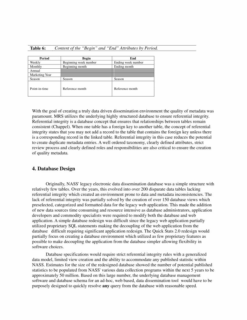
Table 6: Content of the “Begin” and “End” Attributes by Period.

Period Begin End

Weekly Beginning week number Ending week number

Monthly Beginning month Ending month

Annual

Marketing Year

Season Season Season

Point-in-time Reference month Reference month

With the goal of creating a truly data driven dissemination environment the quality of metadata was paramount. MRS utilizes the underlying highly structured database to ensure referential integrity. Referential integrity is a database concept that ensures that relationships between tables remain consistent (Chappel). When one table has a foreign key to another table, the concept of referential integrity states that you may not add a record to the table that contains the foreign key unless there is a corresponding record in the linked table. Referential integrity in this case reduces the potential to create duplicate metadata entries. A well ordered taxonomy, clearly defined attributes, strict review process and clearly defined roles and responsibilities are also critical to ensure the creation of quality metadata.

4. Database Design

Originally, NASS' legacy electronic data dissemination database was a simple structure with relatively few tables. Over the years, this evolved into over 200 disparate data tables lacking referential integrity which created an environment prone to data and metadata inconsistencies. The lack of referential integrity was partially solved by the creation of over 150 database views which preselected, categorized and formatted data for the legacy web application. This made the addition of new data sources time consuming and resource intensive as database administrators, application developers and commodity specialists were required to modify both the database and web application. A simple database redesign was difficult since the legacy web application partially utilized proprietary SQL statements making the decoupling of the web application from the database difficult requiring significant application redesign. The Quick Stats 2.0 redesign would partially focus on creating a database environment which utilized as few proprietary features as possible to make decoupling the application from the database simpler allowing flexibility in software choices.

Database specifications would require strict referential integrity rules with a generalized data model, limited view creation and the ability to accommodate any published statistic within NASS. Estimates for the size of the redesigned database showed the number of potential published statistics to be populated from NASS' various data collection programs within the next 5 years to be approximately 50 million. Based on this large number, the underlying database management software and database schema for an ad-hoc, web based, data dissemination tool would have to be purposely designed to quickly resolve any query from the database with reasonable speed.

Since many web based applications involve transactional processing such as placing orders or updating user information, web developers may be inclined to utilize an OLTP or on-line transactional processing data model or schema. OLTP data models seek to improve transaction performance by utilizing a technique called entity relation modeling removing redundancy within the data. Entity relationship models work by dividing the data into many discrete entities or tables within a database. The tables are then joined with similar attributes with almost every table generally having the ability to be connected in some form to every other table. This creates many potential paths by which to join tables together and the results of those joins, while similar in attributes, may not return the same result. This type of data model allows insert, update and delete transactions to occur quickly, but in an ad-hoc environment where attribute constraint combinations are unknown and large swaths of data are involved generally performs poorly (Kimball).

Dimensional Models or Star Schema can be described as database structures that match the ad-hoc user’s need for simplicity with performance. Dimensional models are generally simple with one large central table containing the “facts” or published statistics in our case and several smaller tables “dimensions” containing the textual representation of attributes used for constraining the query. This is an asymmetrical model where the fact table contains row numbers that are many, many magnitudes greater than the dimensions (Kimball). The fact table will have one join path to each of the dimensions while each dimension only joins to the fact table once. This limited choice of paths guarantees that there can only be one result returned from a given query. In addition to the fact, or published statistic in NASS' case, the fact table contains a set of keys linking the facts back to the various dimension tables. The dimension tables contain the key that joins to the fact and the textual representation a particular attribute to be used. Well designed dimensions will have many well classified attributes that are textually discrete. These attributes will be used as the source of the query constraints while the classifications will be used as the row headers for the users result set. The dimensional model seemed well suited for use in a web based ad-hoc query environment.

The Quick Stats 2.0 dimensional model intentionally followed the design of the aggregate metadata closely utilizing the taxonomies defined in the metadata for simplified browsing. Similar to the organization within MRS, four dimensions were decided upon answering the questions what”,”when”,”where” and additionally “How” with the tables Commodity, Reference Period, Location and Source respectively. Commodity, Location, and Reference Period contains the textual attributes that when combined uniquely describe the “what” of a published estimate. In addition to the textual attributes, each dimension table also contains a surrogate key representing the unique combination of those textual attributes and contains a corresponding entry in the fact table. While upon initial inspection surrogate keys may seem to be simply integers serving as meaningless place holders or links between the fact and the dimensions, their flexibility is significant. The use of surrogate keys would greatly enhance the ability to store any of NASS' published statistics within this data model. Each dimension contains a certain set of attributes that guarantee the uniqueness of that row called the natural key and this will often not be the full set of attributes within a given dimension. Surrogate keys are assigned based upon the uniqueness of a set of natural keys. When populating data, if it is discovered at any time that the natural keys are insufficient to guarantee uniqueness, new attributes can be added to the dimension and included in the set of natural keys, or existing attributes can simply be included in set of natural keys. New surrogate keys will be generated for data to include the new attribute(s), while existing surrogate keys may continue to be used without modification. This creates extreme flexibility within the data model however, there is a cost associated with surrogate keys. When loading data, one of two things must occur; surrogate keys for existing natural keys are looked up or new surrogate keys for new natural key combinations are assigned. Both cases require the additional steps of identifying the surrogate key making data loads slightly more complex.

Figure 2: Quick Stats 2.0 Dimensional Data Model.

Even with a simplified five table dimensional data model (figure 2), previous data warehousing experience at NASS has shown evidence that joining tables was problematic to end users. Application development was also slightly more complex when required to write SQL to join tables. A single normalized, pre-joined view (figure 3) of the fact and dimension tables containing all of the dimensions, textual attributes and fact published statistics were created to resemble an Excel Spreadsheet or SAS dataset with tens of millions of rows of data. This would be the only view of data presented to internal data users and application developers thus, eliminating the need to join the fact and dimension tables.

Figure 3: Quick Stats 2.0 Single Data View.

Q U IC K S T A T S

C O M M O D IT Y _ ID : C O M M O D IT Y . C O M M O D IT Y _ ID

S E C T O R _ D E S C : C O M M O D IT Y . S E C T O R _ D E S C

G R O U P _ D E S C : C O M M O D IT Y . G R O U P _ D E S C

S U B G R O U P _ D E S C : C O M M O D IT Y . S U B G R O U P _ D E S C

C O M M O D IT Y _ D E S C : C O M M O D IT Y . C O M M O D IT Y _ D E S C

C L A S S _ D E S C : C O M M O D IT Y . C L A S S _ D E S C

S T A T IS T IC C A T _ D E S C : C O M M O D IT Y . S T A T IS T IC C A T _ D E S C

U N IT _ D E S C : C O M M O D IT Y . U N IT _ D E S C

P R O D N _ P R A C T IC E _ D E S C : C O M M O D IT Y . P R O D N _ P R A C T IC E _ D E S C

M K T _ P R A C T IC E _ D E S C : C O M M O D IT Y . M K T _ P R A C T IC E _ D E S C

U T IL _ P R A C T IC E _ D E S C : C O M M O D IT Y . U T IL _ P R A C T IC E _ D E S C

D O M A IN _ D E S C : C O M M O D IT Y . D O M A IN _ D E S C

D O M A IN C A T _ D E S C : C O M M O D IT Y . D O M A IN C A T _ D E S C

L O N G _ D E S C : C O M M O D IT Y . L O N G _ D E S C

L O C A T IO N _ ID : L O C A T IO N . L O C A T IO N _ ID

A G G _ L E V E L _ D E S C : L O C A T IO N . A G G _ L E V E L _ D E S C

C O U N T R Y _ N A M E : L O C A T IO N . C O U N T R Y _ N A M E

S T A T E _ F IP S _ C O D E : L O C A T IO N . S T A T E _ F IP S _ C O D E

S T A T E _ A L P H A : L O C A T IO N . S T A T E _ A L P H A

S T A T E _ N A M E : L O C A T IO N . S T A T E _ N A M E

A S D _ D E S C : L O C A T IO N . A S D _ D E S C

C O U N T Y _ N A M E : L O C A T IO N . C O U N T Y _ N A M E

R E G IO N _ D E S C : L O C A T IO N . R E G IO N _ D E S C

R E G IO N _ D E S C 2 : L O C A T IO N . R E G IO N _ D E S C 2

R E G IO N _ C O M M O D IT Y _ D E S C : L O C A T IO N . R E G IO N _ C O M M O D IT Y _ D E S C

M E M B E R _ C O D E : L O C A T IO N . M E M B E R _ C O D E

L O C A T IO N _ D E S C : L O C A T IO N . L O C A T IO N _ D E S C

R E F E R E N C E _ P E R IO D _ ID : R E F E R E N C E _ P E R IO D . R E F E R E N C E _ P E R IO D _ ID

Y E A R : < IN T ( E S T _ Y E A R ) >

C R O P _ Y E A R : R E F E R E N C E _ P E R IO D . C R O P Y E A R

F R E Q _ D E S C : R E F E R E N C E _ P E R IO D . F R E Q _ D E S C

B E G IN _ D E S C : R E F E R E N C E _ P E R IO D . B E G IN _ D E S C

E N D _ D E S C : R E F E R E N C E _ P E R IO D . E N D _ D E S C

P E R IO D _ D E S C : R E F E R E N C E _ P E R IO D . P E R IO D _ D E S C

R E F E R E N C E _ P E R IO D _ D E S C : R E F E R E N C E _ P E R IO D . R E F E R E N C E _ P E R IO D _ D E S C

S O U R C E _ D E S C : S O U R C E . S O U R C E _ D E S C

P U B L IS H E D _ E S T IM A T E : E S T IM A T E S . P U B L IS H E D _ E S T IM A T E

E S T IM A T E : E S T IM A T E S . E S T IM A T E

S O U R C E

S O U R C E _ K E Y : IN TE G E R

S O U R C E _ ID : C H A R (4 )

S O U R C E _ D E S C : V A R C H A R (6 0 )

O R IG IN _ C O D E : C H A R

O R IG IN _ D E S C : V A R C H A R (6 0 )

A C TIV ITY _ C O D E : S M A L L IN T

C O M M O D ITY

C O M M O D ITY _ K E Y : IN TE G E R

C O M M O D ITY _ ID : C H A R (4 8 )

S E C TO R _ C O D E : C H A R (2 )

S E C TO R _ D E S C : V A R C H A R (6 0 )

G R O U P _ C O D E : C H A R (2 )

G R O U P _ D E S C : V A R C H A R (8 0 )

S U B G R O U P _ C O D E : C H A R (2 )

S U B G R O U P _ D E S C : V A R C H A R (8 0 )

C O M M O D ITY _ C O D E : C H A R (3 )

C O M M O D ITY _ D E S C : V A R C H A R (8 0 )

C L A S S _ C O D E : C H A R (4 )

C L A S S _ D E S C : V A R C H A R (1 8 0 )

S TA TIS TIC C A T _ C O D E : C H A R (3 )

S TA TIS TIC C A T _ D E S C : V A R C H A R (8 0 )

M K T_ P R A C TIC E _ C O D E : C H A R (3 )

M K T_ P R A C TIC E _ D E S C : V A R C H A R (1 8 0 )

U TIL _ P R A C TIC E _ C O D E : C H A R (3 )

U TIL _ P R A C TIC E _ D E S C : V A R C H A R (1 8 0 )

P R O D N _ P R A C T IC E _ C O D E : C H A R (3 )

P R O D N _ P R A C T IC E _ D E S C : V A R C H A R (1 8 0 )

U N IT_ C O D E : C H A R (3 )

U N IT_ D E S C : V A R C H A R (6 0 )

D O M A IN _ C O D E : C H A R (4 )

D O M A IN _ D E S C : V A R C H A R (3 0 )

D O M A IN C A T_ C O D E : C H A R (5 )

D O M A IN C A T_ D E S C : V A R C H A R (8 0 )

S H O R T_ C O M M C O D E : C H A R (1 2 )

L O N G _ D E S C : V A R C H A R (2 2 0 )

L O C A TIO N

L O C A TIO N _ K E Y : IN TE G E R

L O C A TIO N _ ID : C H A R (4 0 )

A G G _ L E V E L _ C O D E : C H A R (2 )

A G G _ L E V E L _ D E S C : V A R C H A R (4 0 )

C O U N TR Y _ C O D E : C H A R (4 )

C O U N TR Y _ N A M E : V A R C H A R (6 0 )

R E G IO N _ C O D E : C H A R (4 )

R E G IO N _ D E S C : V A R C H A R (8 0 )

R E G IO N _ D E S C 2 : V A R C H A R (8 0 )

R E G IO N _ C O M M O D ITY _ C O D E : C H A R (1 2 )

R E G IO N _ C O M M O D ITY _ D E S C : V A R C H A R (6 0 )

S T A T E _ F IP S _ C O D E : C H A R (2 )

S T A T E _ A L P H A : C H A R (2 )

S T A T E _ N A M E : V A R C H A R (3 0 )

A S D _ C O D E : C H A R (2 )

A S D _ D E S C : V A R C H A R (6 0 )

C O U N TY _ C O D E : C H A R (3 )

C O U N TY _ N A M E : V A R C H A R (3 0 )

C O N G R _ D IS T R IC T_ C O D E : C H A R (2 )

ZIP _ 5 : C H A R (5 )

W A TE R S H E D _ C O D E : C H A R (8 )

W A TE R S H E D _ D E S C : V A R C H A R (1 2 0 )

L O C A TIO N _ D E S C : V A R C H A R (1 2 0 )

M E M B E R _ C O D E : S M A L L IN T

R E F E R E N C E _ P E R IO D

R E F E R E N C E _ P E R IO D _ K E Y : IN TE G E R

R E F E R E N C E _ P E R IO D _ ID : C H A R (1 1 )

F R E Q _ C O D E : C H A R (2 )

F R E Q _ D E S C : V A R C H A R (3 0 )

B E G IN _ C O D E : C H A R (2 )

B E G IN _ D E S C : V A R C H A R (3 0 )

E N D _ C O D E : C H A R (2 )

E N D _ D E S C : V A R C H A R (3 0 )

P E R IO D _ C O D E : C H A R (2 )

P E R IO D _ D E S C : V A R C H A R (3 0 )

R E F E R E N C E _ P E R IO D _ D E S C : V A R C H A R (4 0 )

E S T_ Y E A R : IN TE G E R

C R O P Y E A R : IN TE G E R

E S TIM A TE S

C O M M O D ITY _ K E Y : IN TE G E R

L O C A TIO N _ K E Y : IN TE G E R

R E F E R E N C E _ P E R IO D _ K E Y : IN TE G E R

S O U R C E _ K E Y : IN TE G E R

P U B L IS H E D _ E S TIM A TE : V A R C H A R (1 2 )

E S TIM A TE : D E C IM A L (1 5 ,4 )

M D 5 S U M : V A R C H A R (3 2 )

L O A D _ F IL E : V A R C H A R (3 0 )

A data warehousing management software from IBM called Red Brick Warehouse has been used by NASS since 1996 to house the reporter level data collected from the US. Census of Agriculture and Survey Programs and currently contains over 7 billion rows of data. Red Brick Warehouse is also ANSI SQL compliant which allows the application developers to satisfy the requirement that the application be database agnostic avoiding lock in with any proprietary database management software. Usage statistics against the Red Brick Warehouse reporter level data warehouse show that over 98% of ad-hoc queries against the 7 billion row fact table resolve in less than 2 seconds and that the general nature of these simple queries was to select or sum a small amount of data with several constraints applied. This type of well constrained query and those needed for an ad-hoc web based query tool (Quick Stats 2.0) would be similar in nature. The indexing and data storage mechanics of Red Brick are also well suited to dimensional data models. These factors lead to the utilization of Red Brick Warehouse for the Quick Stats 2.0 database.

One consideration for data design is to ensure that when users progressively limit data by

adding attributes to constrain result sets the remaining unselected attributes available as constraints are checked for validity. Given the following selection criteria: sector =”CROPS”, year = “2010” and state name = “ARIZONA”, the list of commodities available for selections should only include those with valid data for crops during 2010 in Arizona. To retrieve the list of valid data items the database must join the various dimensions through the fact table to check for the distinct set of valid commodities based on those constraints. While not overly complex, this type of query will need to occur each time a user adds a constraint and must perform well. When checking against 50 million data items this can become time consuming and slow the process of constraining. Red Brick maintains data objects called aggregate tables which are used heavily in the Quick Stats 2.0 database, but not in the traditional sense. Normally aggregate objects are used to sum (aggregate) data to improve query performance. For example, a chain of stores might want to sum all sales for a month in a given region. Having this information summed in an aggregate table maintained at data load can significantly improve performance. Quick Stats 2.0 does not sum data but utilizes aggregate objects that represent various combinations of dimensional attributes to improve the process of constraining data. The above example of crops for 2010 in Arizona could be aided by an aggregate table containing the distinct list of commodities by sector, year, and state name. A balanced set of aggregate tables with the ability to resolve any combination of constraints quickly will greatly improve performance in an ad-hoc environment. An alternative to aggregate tables can be found with the use of a column oriented DBMS where data storage is by column rather than by row. Data warehousing applications can generally benefit from this type of storage as aggregates are computed over large numbers of similar data items. Two open source databases have shown promise as alternatives including Infobright (1) and Calpont’s InfiniDB (2).

5. Application Design

Business specifications for the redesign of Quick Stats were limited to the creation of a generalized, fully ad-hoc, web based, query tool capable of limited mapping and charting functionalities providing users with the ability to customize and save queries.

With a relatively short development time frame, a Rapid Application Development (RAD) environment was chosen for Quick Stats 2.0. RAD refers to a software development methodology favoring minimal specification gathering instead relying on rapid prototyping and iterative development that allows for development to take place at a faster pace. This methodology is well suited for situations where minimal specifications are provided which was the case with Quick Stats 2.0. In RAD, structured techniques and prototyping are utilized to define users' requirements as part of the development process and ultimately used to design the final application (Whitten). The RAD

process begins with development of preliminary data models and business process (controller) models using more structured techniques. Requirements are then verified using iterative development and prototyping refining the data and process models with each iteration. RAD approaches may entail compromises in functionality and performance in exchange for enabling faster development and facilitating application maintenance.

The Quick Stats 2.0 application framework is an open source Model-View-Controller (MVC) called Catalyst that is favored for web applications especially within a RAD environment. The Catalyst framework is written in Perl, designed to simplify the tasks common in web applications, and scales and performs well. Since Catalyst is Perl based, developers have thousands of modules available through the Comprehensive Perl Archive Network (CPAN) to accomplish various tasks. The basic principle of an MVC is to functionally separate the application into three main areas including; processing information (Model), outputting the results (View) and handling application flow or business process (Controller). The areas of the MVC are not only physically separated allowing modification or replacement of one without affecting others; they are also logically separated making code easier to organize. The Model serves to allow access to data, generally a relational database, but can also use other data sources, such as search engines or an Lightweight Directory Access Protocol (LDAP) server. The purpose of the View is to present data to the user typically using a templating module to generate HTML code (Template Toolkit in the case of Quick Stats 2.0), but it's also possible to generate PDF output, send e-mail, etc., from a View. The Controller handles requests within Controller modules determining what a user is trying to do, gather the necessary data from a Model, and send it to a View for display (Diment). Utilizing a MVC allows the application to be generalized by allowing developers to modify one area of the application without affecting the rest the application. For example, the Model can easily be changed to utilize a different database or can be extended to include data for other databases. This allows the application to be generalized and work from a configuration based upon the metadata relationships. With well defined metadata, a generalized configurable application can then be reused with different data sources and in fact the Quick Stats 2.0 application has be used for several different data sources by simply changing the configuration.

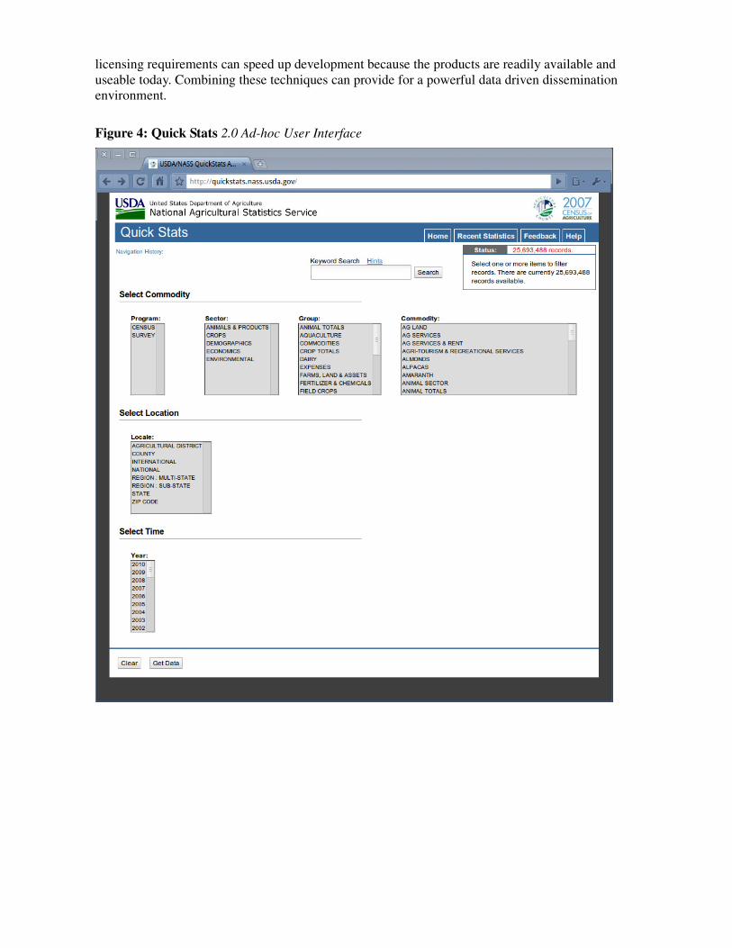
The ad-hoc nature of the Quick Stats 2.0 application involved users making selections from

various pick lists progressively limiting data in order to retrieve their required results. This type of interaction with a web based application benefits greatly from Web 2.0 technologies, namely Asynchronous JavaScript and XML (AJAX). One such open source AJAX framework, the Dojo Toolkit not only contained the necessary AJAX component libraries but also has additional libraries such as the multi-select lists (figure 4.) and a polished interactive data grid (figure 5) making the framework especially useful for data dissemination applications. AJAX programming uses JavaScript to upload and download new data from the web server without undergoing a full page reload. AJAX permits users to interact with objects, such as selections lists, within the page without the need to reload the entire page after each selection. Since data requests going to the server are separated from data being posted back to the page (asynchronously), other select lists can be refreshed with data limited by the first request. This allows the user progressively limit data interactively, seeing immediate results. In turn this provides the ability to explore available data without requesting the actual results. AJAX also increases the overall performance of the site by only updating necessary information rather than updating the entire page.

Dojo's DataGrid is similar to a mini web based spreadsheet making it especially well suited

for electronic data dissemination projects. In HTML terms, the grid is a “super-table” with its own scrollable viewport. One area where the grid excels is in the ability to display large amounts of data by employing a technique called “lazy loading”. The principle behind lazy loading is to only build nodes for records that are viewable. If a user selects a record set with 50,000 rows, they can only view 20 rows at a time on the screen. Lazy loading works by creating the nodes as the user scrolls

so that only visible nodes are created. The grid also features nested sorting, drag and drop functionality, columns reordering, column hiding, and accessibility for screen readers. The Quick Stats 2.0 implementation of the grid also features the ability for users to pivot or cross tabulate data. Figure 5 displays data pivoted by the commodity allowing the users greater flexibility in data presentation.

The interactive mapping requirements (figure 6) were met using MapServer and Open

Layers. MapServer is a Common Gateway Interface (CGI) program residing on the web server which simply creates an image of the requested map. The request may also return images for legends, scale bars, reference maps, and values passed as CGI variables. Open Layers is another open source JavaScript library for displaying the maps created by MapServer. The combination of these two products allows Quick Stats 2.0 to generate maps dynamically based on results from the data grid.

One difficulty in a truly ad-hoc web environment is the ability to deal with potentially large

number constraints. Quick Stats 2.0 currently contains statistics for over 23,000 commodities, 40,000 locations, and 10,000 reference periods. Displaying the potential constraints to the end user is a balancing act as it would be impractical to display a select list with all 23,000 commodities. Quick Stats 2.0 utilizes the metadata taxonomies and parent, child, sibling relationships to determine which constraint lists to initially display and when to present the user with additional constraints. Initially, only the source, sector, group and commodity constraint lists are displayed. After a user has selected one or more items from one of these, they are presented with the data item constraint list. Location operates similarly but only displays valid constraint lists based on the parent child relationships in (table 4). Leveraging the metadata relationships not only allows the application to dynamically display relevant constraint lists, but allows the developers to dynamically create objects based on these relationships.

With a large numbers of constraints possible for any given ad-hoc query and the need to be

able to save these queries, a method to easily store and identify query constraints was required. Unique Universal Identifiers (UUID) is an identification standard that guarantees that with reasonable confidence a set of information can be uniquely identified without central coordination. The UUID consists of 32 hexadecimal digits, separated by hyphens, displayed in 5 groups following the form 8-4-4-4-12 for a total of 36 characters for example “631B5E2C-F4A4-314C-8A3A-E5A8D86642C2”. For any given query within QuickStats 2.0, the UUID along with all of the constraints and the order of which the constraints were selected is stored within a database. This allows for a dataset returned from a query to be identified and reused throughout the application. The data grid, maps, downloadable files and even the initial constraint lists all operate on the UUID. This also allows users to save a query by simply saving a link to the application containing the UUID.

6. Summary

Creating a Web 2.0 based, data warehouse powered data dissemination environment is greatly aided by taking a three phase approach focusing on metadata, database design and application design. Standardizing metadata, developing taxonomies, and classifying attributes provide the ability to automatically generate intuitive text-based navigation. A simplified, generalized database design closely linked to the metadata will allow for broader usage. Database performance is also of importance and should be a top design concern. A well organized yet flexible application framework and iterative development process will speed up time to delivery and ease application maintenance. Open source software can reduce budget requirements and reduced

licensing requirements can speed up development because the products are readily available and useable today. Combining these techniques can provide for a powerful data driven dissemination environment.

Figure 4: Quick Stats 2.0 Ad-hoc User Interface

Figure 5: Quick Stats 2.0 Interactive Data Grid

Figure 6: Quick Stats 2.0 Mapping

REFERENCES

1. Chapple, M (2010) http://databases.about.com/cs/administration/g/refintegrity.htm

2. Diment K., Trout M. (2009) The Definitive Guide to Catalyst: Writing Extendable, Scalable and Maintainable Perl–Based Web Applications

3. Garshol L. (2004) Metadata? Thesauri? Taxonomies? Topic Maps! http://www.ontopia.net/topicmaps/materials/tm-vs-thesauri.html#N429#N429.

4. Kimball, R (1996) The Data Warehouse Toolkit

5. Ricci, C (2004) Developing and Creatively Leveraging Hierarchical Metadata and

Taxonomy

6. Whitten, J; Bentley L, Dittman C. (2004). Systems Analysis and Design Methods. 6th edition.

RESOURCES

1. Infobright : http://infobright.com

2. InfiniDB : http://infinidb.org/

3. Dojo : http://www.dojotoolkit.org/

4. MapServer : http://mapserver.org/

5. Open Layers: http://openlayers.org/

6. Catalyst: http://www.catalystframework.org/