Data Structures and Analysisdavid/course-notes/csc263.pdf · Lecture Notes for CSC263 (Version 0.2)...

David Liu

Data Structures and Analy-sisLecture Notes for CSC263 (Version 0.2)

Department of Computer ScienceUniversity of Toronto

data structures and analysis 3

These notes are based heavily on past offerings of CSC263, and

in particular the materials of François Pitt and Larry Zhang.

I also thank CSC263 students from Fall 2016 and Daniel Zingaro

for pointing out numerous typos in older versions of the notes.

Contents

1 Introduction and analysing running time 7

How do we measure running time? 7

Three different symbols 8

Worst-case analysis 9

1 Introduction and analysing running time

Before we begin our study of different data structures and their applications, weneed to discuss how we will approach this study. In general, we will follow astandard approach:

1. Motivate a new abstract data type or data structure with some examples andreflection of previous knowledge.

2. Introduce a data structure, discussing both its mechanisms for how it storesdata and how it implements operations on this data.

3. Justify why the operations are correct.

4. Analyse the running time performance of these operations.

Given that we all have experience with primitive data structures such as arrays(or Python lists), one might wonder why we need to study data structures at all:can’t we just do everything with arrays and pointers, already available in manylanguages?

Indeed, it is true that any data we want to store and any operation we wantto perform can be done in a programming language using primitive constructssuch as these. The reason we study data structures at all, spending time in-venting and refining more complex ones, is largely because of the performanceimprovements we can hope to gain over their more primitive counterparts.

This is not to say arrays and pointersplay no role. To the contrary, the studyof data structures can be viewed asthe study of how to organize andsynthesize basic programming languagecomponents in new and sophisticatedways.

Given the importance of this performance analysis, it is worth reviewing whatyou already know about how to analyse the running time of algorithms, andpointing out some common misconceptions and subtleties you may have missedalong the way.

How do we measure running time?

As we all know, the amount of time a program or single operation takes to rundepends on a host of external factors — computing hardware, other runningprocesses — over which the programmer has no control.

So, in our analysis, we focus on just one central measure of performance: the re-lationship between an algorithm’s input size and the number of basic operations thealgorithm performs. But because even what is meant by “basic operation” can

8 david liu

differ from machine to machine or programming language to programming lan-guage, we do not try to precisely quantify the exact number of such operations,but instead categorize how the number grows relative to the size of the algorithm’sinput.

This is our motivation for Big-Oh notation, which is used to bring to the fore-ground the type of long-term growth of a function, hiding all the numeric con-stants and smaller terms that do not affect this growth. For example, the func-tions n + 1, 3n− 10, and 0.001n + log n all have the same growth behaviour asn gets large: they all grow roughly linearly with n. Even though these “lines”all have different slopes, we ignore these constants and simply say that thesefunctions are O(n), “Big-Oh of n.”

We will not give the formal definitionof Big-Oh here. For that, please consultthe CSC165 course notes.We call this type of analysis asymptotic analysis, since it deals with the long-term

behaviour of a function. It is important to remember two important facts aboutasymptotic analysis:

• The target of the analysis is always a relationship between the size of the inputand number of basic operations performed.

What we mean by “size of the input” depends on the context, and we’ll alwaysbe very careful when defining input size throughout this course. What wemean by “basic operation” is any operation whose running time does notdepend on the size of the algorithm’s input.

This is deliberately a very liberaldefinition of “basic operation.” Wedon’t want you to get hung up on stepcounting, because that’s completelyhidden by Big-Oh expressions.

• The result of the analysis is a qualitative rate of growth, not an exact numberor even an exact function. We will not say “by our asymptotic analysis, wefind that this algorithm runs in 5 steps” or even “...in 10n + 3 steps.” Rather,expect to read (and write) statements like “we find that this algorithm runsin O(n) time.”

Three different symbols

In practice, programmers (and even theoreticians) tend to use the Big-Oh sym-bol O liberally, even when the precise definition of O is not exactly what weintended. However, in this course it will be important to be precise, and we willactually use three symbols to convey different pieces of information, so you willbe expected to know which one means what. Here is a recap:

• Big-Oh. f = O(g) means that the function f (x) grows slower or at the samerate as g(x). So we can write x2 + x = O(x2), but it is also correct to write

Or, “g is an upper bound on the rate ofgrowth of f .”x2 + x = O(x100) or even x2 + x = O(2x).

• Omega. f = Ω(g) means that the function f (x) grows faster or at the samerate as g(x). So we can write x2 + x = Ω(x2), but it is also correct to write

Or, “g is a lower bound on the rate ofgrowth of f .”x2 + x = Ω(x) or even x2 + x = Ω(log log x).

• Theta. f = Θ(g) means that the function f (x) grows at the same rate as g(x).Or, “g has the same rate of growth asf .”So we can write x2 + x = Θ(x2), but not x2 + x = Θ(2x) or x2 + x = Θ(x).

Note: saying f = Θ(g) is equivalent to saying that f = O(g) and f = Ω(g),i.e., Theta is really an AND of Big-Oh and Omega.


Through unfortunate systemic abuse of notation, most of the time when a com-puter scientist says an algorithm runs in “Big-Oh of f time,” she really means“Theta of f time.” In other words, that the function f is not just an upper boundon the rate of growth of the running time of the algorithm, but is in fact therate of growth. The reason we get away with doing so is that in practice, the“obvious” upper bound is in fact the rate of growth, and so it is (accidentally)correct to mean Theta even if one has only thought about Big-Oh.

However, the devil is in the details: it is not the case in this course that the“obvious” upper bound will always be the actual rate of growth, and so we willsay Big-Oh when we mean an upper bound, and treat Theta with the reverenceit deserves. Let us think a bit more carefully about why we need this distinction.

Worst-case analysis

The procedure of asymptotic analysis seems simple enough: look at a piece ofcode; count the number of basic operations performed in terms of the input size,

remember, a basic operation is anyoperation whose runtime doesn’tdepend on the input size

taking into account loops, helper functions, and recursive calls; then convert thatexpression into the appropriate Theta form.

Given any exact mathematical function, it is always possible to determine itsqualitative rate of growth, i.e., its corresponding Theta expression. For example,the function f (x) = 300x5 − 4x3 + x + 10 is Θ(x5), and that is not hard to figureout.

So then why do we need Big-Oh and Omega at all? Why can’t we always just godirectly from the f (x) expression to the Theta?

It’s because we cannot always take a piece of code an come up with an exactexpression for the number of basic operations performed. Even if we take theinput size as a variable (e.g., n) and use it in our counting, we cannot alwaysdetermine which basic operations will be performed. This is because input sizealone is not the only determinant of an algorithm’s running time: often the valueof the input matters as well.

Consider, for example, a function that takes a list and returns whether this listcontains the number 263. If this function loops through the list starting at thefront, and stops immediately if it finds an occurrence of 263, then in fact the run-ning time of this function depends not just on how long the list is, but whetherand where it has any 263 entries.

Asymptotic notations alone cannot help solve this problem: they help us clar-ify how we are counting, but we have here a problem of what exactly we arecounting.

This problem is why asymptotic analysis is typically specialized to worst-caseanalysis. Whereas asymptotic analysis studies the relationship between inputsize and running time, worst-case analysis studies only the relationship betweeninput size of maximum possible running time. In other words, rather than an-swering the question “what is the running time of this algorithm for an input

10 david liu

size n?” we instead aim to answer the question “what is the maximum possiblerunning time of this algorithm for an input size n?” The first question’s answermight be a whole range of values; the second question’s answer can only be asingle number, and that’s how we get a function involving n.

Some notation: we typically use the name T(n) to represent the maximum pos-sible running time as a function of n, the input size. The result of our analysiscould be something like T(n) = Θ(n), meaning that the worst-case running timeof our algorithm grows linearly with the input size.

Bounding the worst case

But we still haven’t answered the question: where do O and Ω come in? Theanswer is basically the same as before: even with our restricted focus on worst-case running time, it is not always possible to calculate an exact expression forthis function. What is usually easy to do, however, is calculate an upper boundon the maximum number of operations. One such example is the likely familiarline of reasoning, “the loop will run at most n times” when searching for 263 ina list of length n. Such analysis, which gives a pessimistic outlook on the mostnumber of operations that could theoretically happen, results in an exact count— e.g., n + 1 — which is an upper bound on the maximum number of operations.From this analysis, we can conclude that T(n), the worst-case running time, isO(n).

What we can’t conclude is that T(n) = Ω(n). There is a subtle implicationhere of the English phrase “at most.” When we say “you can have at most10 chocolates,” it is generally understood that you can indeed have exactly 10

chocolates; whatever number is associated with “at most” is achievable.

In our analysis, however, we have no way of knowing that the upper boundwe obtain by being pessimistic in our operation counting is actually achievable.This is made more obvious if we explicitly mention the fact that we’re studyingthe maximum possible number of operations: “the maximum running time isless than or equal to n + 1” surely says something different than “the maximumrunning time is equal to n + 1.”

So how do we show that whatever upper bound we get on the maximum isactually achievable? In practice, we rarely try to show that the exact upperbound is achievable, since that doesn’t actually matter. Instead, we try to showthat an asymptotic lower bound — an Omega — is achievable. For example, wemight want to show that the maximum running time is Ω(n), i.e., grows at leastas quickly as n.

To show that the maximum running time grows at least as quickly as some func-tion f , we need to find a family of inputs, one for each input size n, whose run-ning time has a lower bound of f (n). For example, for our problem of searchingfor 263 in a list, we could say that the family of inputs is “lists that contain only0’s.” Running the search algorithm on such a list of length n certainly requireschecking each element, and so the algorithm takes at least n basic operations.From this we can conclude that the maximum possible running time is Ω(n).

Remember, the constants don’t matter.The family of inputs that contain only1’s for the first half, and only 263’s forthe second half, would also have givenus the desired lower bound.


To summarize: to perform a complete worst-case analysis and get a tight, Thetabound on the worst-case running time, we need to do the following two things:

(i) Give a pessimistic upper bound on the number of basic operations that couldoccur for any input of a fixed size n. Obtain the corresponding Big-Oh expres-sion (i.e., T(n) = O( f )).

Observe that (i) is proving somethingabout all possible inputs, while (ii) isproving something about just one familyof inputs.

(ii) Give a family of inputs (one for each input size), and give a lower bound on thenumber of basic operations that occurs for this particular family of inputs.Obtain the corresponding Omega expression (i.e., T(n) = Ω( f )).

If you have performed a careful analysis in (i) and chosen a good family in(ii), then you’ll find that the Big-Oh and Omega expressions involve the samefunction f , and which point you can conclude that the worst-case running timeis T(n) = Θ( f ).

Average-case analysis

So far in your career as computer scientists, you have been primarily concernedwith worst-case algorithm analysis. However, in practice this type of analysisoften ends up being misleading, with a variety of algorithms and data structureshaving a poor worst-case performance still performing well on the majority ofpossible inputs.

Some reflection makes this not too surprising: focusing on the maximum of aset of numbers (like running times) says very little about the “typical” numberin that set, or, more precisely, the distribution of numbers within that set. In thissection, we will learn a powerful new technique that enables us to analyse somenotion of “typical” running time for an algorithm.

Warmup

Consider the following algorithm, which operates on a non-empty array of inte-gers:

1 def evens_are_bad(lst):

2 if every number in lst is even:

3 repeat lst.length times:

4 calculate and print the sum of lst

5 return 1

6 else:

7 return 0

Let n represent the length of the input list lst. Suppose that lst contains onlyeven numbers. Then the initial check on line 2 takes Ω(n) time, while the com-putation in the if branch takes Ω(n2) time. This means that the worst-case

We leave it as an exercise to justify whythe if branch takes Ω(n2) time.

12 david liu

running time of this algorithm is Ω(n2). It is not too hard to prove the matchingupper bound, and so the worst-case running time is Θ(n2).

However, the loop only executes when every number in lst is even; when justone number is odd, the running time is O(n), the maximum possible runningtime of executing the all-even check. Intuitively, it seems much more likely that

Because executing the check mightabort quickly if it finds an odd numberearly in the list, we used the pessimisticupper bound of O(n) rather than Θ(n).

not every number in lst is even, so we expect the more “typical case” for thisalgorithm is to have a running time bounded above by O(n), and only veryrarely to have a running time of Θ(n2).

Our goal now is to define precisely what we mean by the “typical case” for analgorithm’s running time when considering a set of inputs. As is often the casewhen dealing with the distribution of a quantity (like running time) over a setof possible values, we will use our tools from probability theory to help achievethis goal.

We define the average-case running time of an algorithm to be the functionTavg(n) which takes a number n and returns the (weighted) average of the algo-rithm’s running time for all inputs of size n.

For now, let’s ignore the “weighted” part, and just think of Tavg(n) as computingthe average of a set of numbers. What can we say about the average-case for thefunction evens_are_bad? First, we fix some input size n. We want to computethe average of all running times over all input lists of length n.

At this point you might be thinking, “well, each number is even with probabilityone-half, so...” This is a nice thought, but a little premature – the first stepwhen doing an average-case analysis is to define the possible set of inputs.For this example, we’ll start with a particularly simple set of inputs: the listswhose elements are between 1 and 5, inclusive. The reason for choosing such arestricted set is to simplify the calculations we need to perform when computingan average.

As the calculation requires precise numbers, we will need to be precise aboutwhat “basic operations” we’re counting. For this example, we’ll count only thenumber of times a list element is accessed, either to check whether it is even,or when computing the sum of the list. So a “step” will be synonymous with“list access.”

It is actually fairly realistic to focussolely on operations of a particulartype in a runtime analysis. We typicallychoose the operation that happens themost frequently (as in this case), orthe one which is the most expensive.Of course, the latter requires that weare intimately knowledgeable aboutthe low-level details of our computingenvironment.

The preceding paragraphs are the work of setting up the context of our analysis:what inputs we’re considering, and how we’re measuring runtime. The finalstep is what we had initially talked about: compute the average running timeover inputs of length n. This often requires some calculation, so let’s get to it.To simplify our calculations even further, we’ll assume that the all-evens checkon line 2 always accesses all n elements. In the loop, there are n2 steps (each

You’ll explore the “return early” variantin an exercise.number is accessed n times, once per time the sum is computed).

There are really only two possibilities: the lists that have all even numbers willrun in n2 + n steps, while all the other lists will run in just n steps. How manyof each type of list are there? For each position, there are two possible evennumbers (2 and 4), so the number of lists of length n with every element beingeven is 2n. That sounds like a lot, but consider that there are five possible values

In the language of counting: maken independent decisions, with eachdecision having two choices.


per element, and hence 5n possible inputs in all. So 2n inputs have all evennumbers and take n2 + n steps, while the remaining 5n − 2n inputs take n steps.

Number Stepsall even 2n n2 + nthe rest 5n − 2n n

The average running time is:

Tavg(n) =2n(n2 + n) + (5n − 2n)n

5n (5n inputs total)

=2nn2

5n + n

=

(25

)nn2 + n

= Θ(n) Remember that any exponential growsfaster than any polynomial, so the firstterm goes to 0 as n goes to infinity.

This analysis tells us that the average-case running time of this algorithm isΘ(n), as our intuition originally told us. Because we computed an exact expres-sion for the average number of steps, we could convert this directly into a Thetaexpression.

As is the case with worst-case analysis,it won’t always be so easy to computean exact expression for the average,and in those cases the usual upper andlower bounding must be done.

The probabilistic view

The analysis we performed in the previous section was done through the lensof counting the different kinds of inputs and then computing the average oftheir running times. However, there is a more powerful technique: treating thealgorithm’s running time as a random variable T, defined over the set of possibleinputs of size n. We can then redo the above analysis in this probabilistic context,performing these steps:

1. Define the set of possible inputs and a probability distribution over this set. Inthis case, our set is all lists of length n that contain only elements in therange 1-5, and the probability distribution is the uniform distribution.

Recall that the uniform distributionassigns equal probability to eachelement in the set.

2. Define how we are measuring runtime. (This is unchanged from the previousanalysis.)

3. Define the random variable T over this probability space to represent therunning time of the algorithm.

Recall that a random variable is afunction whose domain is the set ofinputs.

In this case, we have the nice definition

T =

n2 + n, input contains only even numbers

n, otherwise

4. Compute the expected value of T, using the chosen probability distributionand formula for T. Recall that the expected value of a variable is determinedby taking the sum of the possible values of T, each weighted by the probabilityof obtaining that value.

E[T] = ∑t

t · Pr[T = t]

14 david liu

In this case, there are only two possible values for T:

E[T] = (n2 + n) · Pr[the list contains only even numbers]

+ n · Pr[the list contains at least one odd number]

= (n2 + n) ·(

25

)n+ n ·

(1−

(25

)n)= n2 ·

(25

)n+ n

= Θ(n)

Of course, the calculation ended up being the same, even if we approached ita little differently. The point to shifting to using probabilities is in unlockingthe ability to change the probability distribution. Remember that our first step,defining the set of inputs and probability distribution, is a great responsibilityof the ones performing the runtime analysis. How in the world can we choosea “reasonable” distribution? There is a tendency for us to choose distributions

What does it mean for a distribution tobe “reasonable,” anyway?that are easy to analyse, but of course this is not necessarily a good criterion for

evaluating an algorithm.

By allowing ourselves to choose not only what inputs are allowed, but also giverelative probabilities of those inputs, we can use the exact same technique toanalyse an algorithm under several different possible scenarios. This is both thereason we use “weighted average” rather than simply “average” in our abovedefinition of average-case, and also how we are able to calculate it.

Exercise Break!

1.1 Prove that the evens_are_bad algorithm on page 11 has a worst-case runningtime of O(n2), where n is the length of the input list.

1.2 Consider this alternate input space for evens_are_bad: each element in thelist is even with probability 99

100 , independent of all other elements. Prove thatunder this distribution, the average-case running time is still Θ(n).

1.3 Suppose we allow the “all-evens” check on line 2 of evens_are_bad to stopimmediately after it finds an odd element. Perform a new average-case anal-ysis for this mildly-optimized version of the algorithm using the same inputdistribution as in the notes.

Hint: part of the running time T now can take on any value between 1 and n;first compute the probability of getting each of these values, and then use theexpected value formula.

Quicksort is fast on average

The previous example may have been a little underwhelming, since it was “ob-vious” that the worst-case was quite rare, and so not surprising that the average-case running time is asymptotically faster than the worst-case. However, this is


not a fact you should take for granted. Indeed, it is often the case that algorithmsare asymptotically no better “on average” than they are in the worst-case. Some-

Keep in mind that because asymptoticnotation hides the constants, saying twofunctions are different asymptotically ismuch more significant than saying thatone function is “bigger” than another.

times, though, an algorithm can have a significantly better average case thanworst case, but it is not nearly as obvious; we’ll finish off this chapter by study-ing one particularly well-known example.

Recall the quicksort algorithm, which takes a list and sorts it by choosing oneelement to be the pivot (say, the first element); partitioning the remaining ele-ments into two parts, those less than the pivot, and those greater than the pivot;recursively sorting each part; and then combining the results.

1 def quicksort(array):

2 if array.length < 2:

3 return

4 else:

5 pivot = array[0]

6 smaller, bigger = partition(array[1:], pivot)

7 quicksort(smaller)

8 quicksort(bigger)

9 array = smaller + [pivot] + bigger # array concatenation

10

11 def partition(array, pivot):

12 smaller = []

13 bigger = []

14 for item in array:

15 if item <= pivot:

16 smaller.append(item)

17 else:

18 bigger.append(item)

19 return smaller, bigger

This version of quicksort uses linear-size auxiliary storage; we chose thisbecause it is a little simpler to writeand analyse. The more standard “in-place” version of quicksort has thesame running time behaviour, it justuses less space.

You have seen in previous courses that the choice of pivot is crucial, as it de-termines the size of each of the two partitions. In the best case, the pivot is themedian, and the remaining elements are split into partitions of roughly equalsize, leading to a running time of Θ(n log n), where n is the size of the list.However, if the pivot is always chosen to be the maximum element, then thealgorithm must recurse on a partition that is only one element smaller than theoriginal, leading to a running time of Θ(n2).

So, given that there is a difference between the best- and worst-case runningtimes of quicksort, the next natural question to ask is: What is the average-caserunning time? This is what we’ll answer in this section.

First, let n be the length of the list. Our set of inputs is all possible permutationsof the numbers 1 to n (inclusive). We’ll assume any of these n! permutations

Our analysis will therefore assume thelists have no duplicates.are equally likely; in other words, we’ll use the uniform distribution over all

possible permutations of 1, . . . , n. We will measure runtime by counting thenumber of comparisons between elements in the list in the partition function.

16 david liu

Let T be the random variable counting the number of comparisons made. Beforestarting the computation of E[T], we define additional random variables: foreach i, j ∈ 1, . . . , n with i < j, let Xij be the indicator random variable definedas:

Xij =

1, if i and j are compared

0, otherwise

Because each pair is compared at most once, we obtain the total number ofRemember, this is all in the context ofchoosing a random permutation.

comparisons simply by adding these up:

T =n

∑i=1

n

∑j=i+1

Xij.

The purpose of decomposing T into a sum of simpler random variables is thatwe can now apply the linearity of expectation (see margin note).

If X, Y, and Z are random variables andX = Y + Z, then E[X] = E[Y] + E[Z],even if Y and Z are dependent.

E[T] =n

∑i=1

n

∑j=i+1

E[Xij]

=n

∑i=1

n

∑j=i+1

Pr[i and j are compared] Recall that for an indicator randomvariable, its expected value is simplythe probability that it takes on the value1.

To make use of this “simpler” form, we need to investigate the probability thati and j are compared when we run quicksort on a random array.

Proposition 1.1. Let 1 ≤ i < j ≤ n. The probability that i and j are comparedwhen running quicksort on a random permutation of 1, . . . , n is 2/(j− i + 1).

Proof. First, let us think about precisely when elements are compared with eachother in quicksort. Quicksort works by selecting a pivot element, then comparingthe pivot to every other item to create two partitions, and then recursing on eachpartition separately. So we can make the following observations:

(i) Every comparison must involve the “current” pivot.

(ii) The pivot is only compared to the items that have always been placed into thesame partition as it by all previous pivots.

Or, once two items have been put intodifferent partitions, they will never becompared.So in order for i and j to be compared, one of them must be chosen as the

pivot while the other is in the same partition. What could cause i and j to bein different partitions? This only happens if one of the numbers between i andj (exclusive) is chosen as a pivot before i or j is chosen. So then i and j arecompared by quicksort if and only if one of them is selected to be pivot first outof the set of numbers i, i + 1, . . . , j.

Because we’ve given an implementation of quicksort that always chooses the firstitem to be the pivot, the item that is chosen first as pivot must be the one thatappears first in the random input permutation. Since we choose the permutation

Of course, the input list contains othernumbers, but because our partitionalgorithm preserves relative orderwithin a partition, if a appears beforeb in the original list, then a will stillappear before b in every subsequentpartition that contains them both.


uniformly at random, each item in the set i, . . . , j is equally likely to appearfirst, and thus be chosen first as pivot.

Finally, because there are j− i + 1 numbers in this set, the probability that eitheri or j is chosen first is 2/(j− i + 1), and this is the probability that i and j arecompared.

Now that we have this probability computed, we can return to our expectedvalue calculation to complete our average-case analysis.

Theorem 1.2 (Quicksort average-case runtime). The average number of com-parisons made by quicksort on a uniformly chosen random permutation of1, . . . , n is Θ(n log n).

Proof. As before, let T be the random variable representing the running time ofquicksort. Our previous calculations together show that

E[T] =n

∑i=1

n

∑j=i+1

Pr[i and j are compared]

=n

∑i=1

n

∑j=i+1

2j− i + 1

=n

∑i=1

n−i

∑j′=1

2j′ + 1

(change of index j′ = j− i)

= 2n

∑i=1

n−i

∑j′=1

1j′ + 1 i j′ values

1 1, 2, 3, . . . , n− 2, n− 12 1, 2, 3, . . . , n− 2...

...n− 3 1, 2, 3n− 2 1, 2n− 1 1

n

Now, note that the individual terms of the inner summation don’t depend on i;only the bound does. The first term, when j′ = 1, occurs when 1 ≤ i ≤ n− 1,or n− 1 times in total; the second (j′ = 2) occurs when i ≤ n− 2, and in generalthe j′ = k term appears n− k times.

So we can simplify the counting to eliminate the summation over i:

E[T] = 2n−1

∑j′=1

n− j′

j′ + 1

= 2n−1

∑j′=1

(n + 1j′ + 1

− 1)

= 2(n + 1)n−1

∑j′=1

1j′ + 1

− 2(n− 1)

We will use the fact from mathematics that the function ∑n−1i=1

1i+1 is Θ(log n),

Actually, we even know the exactconstant hidden in the Θ: Look up theHarmonic series if you’re interested inlearning more!

and so we get that E[T] = Θ(n log n).

18 david liu

Exercise Break!

1.4 Review the insertion sort algorithm, which builds up a sorted list by repeat-edly inserting new elements into a sorted sublist (usually at the front). Weknow that its worst-case running time is Θ(n2), but its best case is Θ(n), evenbetter than quicksort. So, does it beat quicksort on average?

Suppose we run insertion sort on a random permutation of the numbers1, . . . , n, and consider counting the number of swaps as the running time.Let T be the random variable representing the total number of swaps.

(a) For each 1 ≤ i ≤ n, define the random variable Si to be the number ofswaps made when i is inserted into the sorted sublist.

Express T in terms of Si.

(b) For each 1 ≤ i, j ≤ n, define the random indicator variables Xij that is 1 if iand j are swapped during insertion sort.

Express Si in terms of the Xij.

(c) Prove that E[Xij] = 1/2.

(d) Show that the average-case running time of insertion sort is Θ(n2).

2 Priority Queues and Heaps

In this chapter, we will study our first major data structure: the heap. As thisis our first extended analysis of a new data structure, it is important to payattention to the four components of this study outlined at the previous chapter:

1. Motivate a new abstract data type or data structure with some examples andreflection of previous knowledge.

2. Introduce a data structure, discussing both its mechanisms for how it storesdata and how it implements operations on this data.

3. Justify why the operations are correct.

4. Analyse the running time performance of these operations.

Abstract data type vs. data structure

The study of data structures involves two principal, connected pieces: a speci-fication of what data we want to store and operations we want to support, andan implementation of this data type. We tend to blur the line between thesetwo components, but the difference between them is fundamental, and we oftenspeak of one independently of the other. So before we jump into our first majordata structure, let us remind ourselves of the difference between these two.

Definition 2.1 (abstract data type, data structure). An abstract data type (ADT)is a theoretical model of an entity and the set of operations that can be performedon that entity.

The key term is abstract: an ADT is adefinition that can be understood andcommunicated without any code at all.A data structure is a value in a program which can be used to store and operate

on data.

For example, contrast the difference between the List ADT and an array datastructure.

List ADT

• Length(L): Return the number of items in L.

• Get(L, i): Return the item stored at index i in L.

• Store(L, i, x): Store the item x at index i in L.

20 david liu

There may be other operations youthink are fundamental to lists; we’vegiven as bare-bones a definition aspossible.

This definition of the List ADT is clearly abstract: it specifies what the possibleoperations are for this data type, but says nothing at all about how the data isstored, or how the operations are performed.

It may be tempting to think of ADTs as the definition of interfaces or abstractclasses in a programming language – something that specifies a collection ofmethods that must be implemented – but keep in mind that it is not necessaryto represent an ADT in code. A written description of the ADT, such as the onewe gave above, is perfectly acceptable.

On the other hand, a data structure is tied fundamentally to code. It exists asan entity in a program; when we talk about data structures, we talk about howwe write the code to implement them. We are aware of not just what these datastructures do, but how they do them.

When we discuss arrays, for example, we can say that they implement the ListADT; i.e., they support the operations defined in the List ADT. However, we cansay much more than this:

• Arrays store elements in consecutive locations in memory

• They perform Get and Store in constant time with respect to the length ofthe array.

• How Length is supported is itself an implementation detail specific to aparticular language. In C, arrays must be wrapped in a struct to manuallystore their length; in Java, arrays have a special immutable attribute calledlength; in Python, native lists are implemented using arrays an a member to

At least, the standard CPython imple-mentation of Python.store length.

The main implementation-level detail that we’ll care about this in course is therunning time of an operation. This is not a quantity that can be specified in thedefinition of an ADT, but is certainly something we can study if we know howan operation is implemented in a particular data structure.

The Priority Queue ADT

The first abstract data type we will study is the Priority Queue, which is similarin spirit to the stacks and queues that you have previously studied. Like thosedata types, the priority queue supports adding and removing an item from acollection. Unlike those data types, the order in which items are removed doesnot depend on the order in which they are added, but rather depends on apriority which is specified when each item is added.

A classic example of priority queues in practice is a hospital waiting room: moresevere injuries and illnesses are generally treated before minor ones, regardlessof when the patients arrived at the hospital.

Priority Queue ADT


• Insert(PQ, x, priority): Add x to the priority queue PQ with the given prior-ity.

• FindMax(PQ): Return the item in PQ with the highest priority.

• ExtractMax(PQ): Remove and return the item from PQ with the highestpriority.

As we have already discussed, one of the biggest themes of this course is the dis-tinction between the definition of an abstract data type, and the implementationof that data type using a particular data structure. To emphasize that these are

One can view most hospital waitingrooms as a physical, buggy implemen-tation of a priority queue.

separate, we will first give a naïve implementation of the Priority Queue ADTthat is perfectly correct, but inefficient. Then, we will contrast this approachwith one that uses the heap data structure.

A basic implementation

Let us consider using an unsorted linked list to implement a priority queue. Inthis case, adding a new item to the priority queue can be done in constant time:simply add the item and corresponding priority to the front of the linked list.However, in order to find or remove the item with the lowest priority, we mustsearch through the entire list, which is a linear-time operation.

Given a new ADT, it is often helpful to come up with a “naïve” or “brute force”implementation using familiar primitive data structures like arrays and linkedlists. Such implementations are usually quick to come up with, and analysingthe running time of the operations is also usually straight-forward. Doing thisanalysis gives us targets to beat: given that we can code up an implementationof priority queue which supports Insert in Θ(1) time and FindMax and Ex-tractMax in Θ(n) time, can we do better using a more complex data structure?The rest of this chapter is devoted to answering this question.

26 def Insert(PQ, x, priority):

27 n = Node(x, priority)

28 oldHead = PQ.head

29 n.next = old_head

30 PQ.head = n

31

32

33 def FindMax(PQ):

34 n = PQ.head

35 maxNode = None

36 while n is not None:

37 if maxNode is None or n.priority > maxNode.priority:

38 maxNode = n

39 n = n.next

40 return maxNode.item

41

42

43 def ExtractMax(PQ):

22 david liu

44 n = PQ.head

45 prev = None

46 maxNode = None

47 prevMaxNode = None

48 while n is not None:

49 if maxNode is None or n.priority > maxNode.priority:

50 maxNode, prevMaxNode = n, prevNode

51 prev, n = n, n.next

52

53 if prevMaxNode is None:

54 self.head = maxNode.next

55 else:

56 prevMaxNode.next = maxNode.next

57

58 return maxNode.item

Heaps

Recall that a binary tree is a tree in which every node has at most two children,which we distinguish by calling the left and right. You probably rememberstudying binary search trees, a particular application of a binary tree that cansupport fast insertion, deletion, and search.

We’ll look at a more advanced form ofbinary search trees in the next chapter.

Unfortunately, this particular variant of binary trees does not exactly suit ourpurposes, since the item with the highest priority will generally be at or nearthe bottom of a BST. Instead, we will focus on a variation of binary trees thatuses the following property:

Definition 2.2 (heap property). A tree satisfies the heap property if and only iffor each node in the tree, the value of that node is greater than or equal to thevalue of all of its descendants.

Alternatively, for any pair of nodes a, b in the tree, if a is an ancestor of b, thenthe value of a is greater than or equal to the value of b.

This property is actually less stringent than the BST property: given a nodewhich satisfies the heap property, we cannot conclude anything about the rela-tionships between its left and right subtrees. This means that it is actually mucheasier to get a compact, balanced binary tree that satisfies the heap propertythan one that satisfies the BST property. In fact, we can get away with enforcingas strong a balancing as possible for our data structure.

Definition 2.3 (complete binary tree). A binary tree is complete if and only if itsatisfies the following two properties:

• All of its levels are full, except possibly the bottom one.Every leaf must be in one of the twobottommost levels.


• All of the nodes in the bottom level are as far to the left as possible.

A

B C

D E F

Complete trees are essentially the trees which are most “compact.” A completetree with n nodes has dlog ne height, which is the smallest possible height for atree with this number of nodes.

Moreover, because we also specify that the nodes in the bottom layer must be asfar left as possible, there is never any ambiguity about where the “empty” spotsin a complete tree are. There is only one complete tree shape for each number of nodes.

Because of this, we do not need to use up space to store references betweennodes, as we do in a standard binary tree implementation. Instead, we fix aconventional ordering of the nodes in the heap, and then simply write down theitems in the heap according to that order. The order we use is called level order,because it orders the elements based on their depth in the tree: the first node isthe root of the tree, then its children (at depth 1) in left-to-right order, then allnodes at depth 2 in left-to-right order, etc.

The array representation of the abovecomplete binary tree.

A B C D E FWith these two definitions in mind, we can now define a heap.

Definition 2.4 (heap). A heap is a binary tree that satisfies the heap property andis complete.

We implement a heap in a program as an array, where the items in the arraycorrespond to the level order of the actual binary tree.

This is a nice example of how we useprimitive data structures to buildmore complex ones. Indeed, a heap isnothing sophisticated from a technicalstandpoint; it is merely an array whosevalues are ordered in a particular way.

A note about array indices

In addition to being a more compact representation of a complete binary tree,this array representation has a beautiful relationship between the indices of anode in the tree and those of its children.

We assume the items are stored starting at index 1 rather than 0, which leads tothe following indices for the nodes in the tree.

1

2 3

4 5 6 7

8 9 10 11 12

We are showing the indices where eachnode would be stored in the array.

A pattern quickly emerges. For a node corresponding to index i, its left child isstored at index 2i, and its right child is stored at index 2i + 1. Going backwards,we can also deduce that the parent of index i (when i > 1) is stored at indexbi/2c. This relationship between indices will prove very useful in the followingsection when we start performing more complex operations on heaps.

Heap implementation of a priority queue

Now that we have defined the heap data structure, let us see how to use it toimplement the three operations of a priority queue.

FindMax becomes very simple to both implement and analyse, because the rootof the heap is always the item with the maximum priority, and in turn is alwaysstored at the front of the array.

Remember that indexing starts at 1

rather than 0.

24 david liu

1 def FindMax(PQ):

2 return PQ[1]

Remove is a little more challenging. Obviously we need to remove the root ofthe tree, but how do we decide what to replace it with? One key observation isthat because the resulting heap must still be complete, we know how its structuremust change: the very last (rightmost) leaf must no longer appear.


Rightmost leaf 17 is moved to the root.

50

30 45

28 20 16 2

8 19 17

17 is swapped with 45 (since 45 isgreater than 30).

17

30 45

28 20 16 2

8 19

So our first step is to save the root of the tree, and then replace it with the lastleaf. (Note that we can access the leaf in constant time because we know the sizeof the heap, and the last leaf is always at the end of the list of items.)

No more swaps occur; 17 is greaterthan both 16 and 2.

45

30 17

28 20 16 2

8 19

But the last leaf priority is smaller than many other priorities, and so if weleave the heap like this, the heap property will be violated. Our last step is torepeatedly swap the moved value with one of its children until the heap propertyis satisfied once more. On each swap, we choose the larger of the two childrento ensure that the heap property is preserved.

The repeated swapping is colloquiallycalled the “bubble down” step, refer-ring to how the last leaf starts at thetop of the heap and makes its way backdown in the loop.

29 def ExtractMax(PQ):

30 temp = PQ[1]

31 PQ[1] = PQ[PQ.size] # Replace the root with the last leaf

32 PQ.size = PQ.size - 1

33

34 # Bubble down

35 i = 1

36 while i < PQ.size:

37 curr_p = PQ[i].priority

38 left_p = PQ[2*i].priority

39 right_p = PQ[2*i + 1].priority

40

41 # heap property is satisfied

42 if curr_p >= left_p and curr_p >= right_p:

43 break

44 # left child has higher priority

45 else if left_p >= right_p:

46 PQ[i], PQ[2*i] = PQ[2*i], PQ[i]

47 i = 2*i

48 # right child has higher priority

49 else:

50 PQ[i], PQ[2*i + 1] = PQ[2*i + 1], PQ[i]

51 i = 2*i + 1

52

53 return temp

What is the running time of this algorithm? All individual lines of code takeconstant time, meaning the runtime is determined by the number of loop itera-tions.

At each iteration, either the loop stops immediately, or i increases by at least afactor of 2. This means that the total number of iterations is at most log n, wheren is the number of items in the heap. The worst-case running time of Remove

is therefore O(log n).

The implementation of Insert is similar. We again use the fact that the numberof items in the heap completely determines its structure: in this case, because a

26 david liu

new item is being added, there will be a new leaf immediately to the right ofthe current final leaf, and this corresponds to the next open position in the arrayafter the last item.

So our algorithm simply puts the new item there, and then performs an inverseof the swapping from last time, comparing the new item with its parent, andswapping if it has a larger priority. The margin diagrams show the result ofadding 35 to the given heap.

A “bubble up” instead of “bubbledown”

45

30 17

28 20 16 2

8 19 35

45

30 17

28 35 16 2

8 19 20

45

35 17

28 30 16 2

8 19 20

35 is swapped twice with its parent (20,then 30), but does not get swapped with45.

56 def Insert(PQ, x, priority):

57 PQ.size = PQ.size + 1

58 PQ[PQ.size].item = x

59 PQ[PQ.size].priority = priority

60

61 i = PQ.size

62 while i > 1:

63 curr_p = PQ[i].priority

64 parent_p = PQ[i // 2].priority

65

66 if curr_p <= parent_p: # heap property satisfied, break

67 break

68 else:

69 PQ[i], PQ[i // 2] = PQ[i // 2], PQ[i]

70 i = i // 2

Again, this loop runs at most log n iterations, where n is the number of items inthe heap. The worst-case running time of this algorithm is therefore O(log n).

Runtime summary

Let us compare the worst-case running times for the three operations for the twodifferent implementations we discussed in this chapter. In this table, n refers tothe number of elements in the priority queue.

Operation Linked list HeapInsert Θ(1) Θ(log n)

FindMax Θ(n) Θ(1)ExtractMax Θ(n) Θ(log n)

This table nicely illustrates the tradeoffs generally found in data structure designand implementation. We can see that heaps beat unsorted linked lists in two ofthe three priority queue operations, but are asymptotically slower than unsortedlinked lists when adding a new element. Now, this particular case is not muchof a choice: that the slowest operation for heaps runs in Θ(log n) time in theworst case is substantially better than the corresponding Θ(n) time for unsortedlinked lists, and in practice heaps are indeed widely used.

The reason for the speed of the heap operations is the two properties – theheap property and completeness – that are enforced by the heap data structures.These properties impose a structure on the data that allows us to more quicklyextract the desired information. The cost of these properties is that they mustbe maintained whenever the data structure is mutated. It is not enough to take


a new item and add it to the end of the heap array; it must be “bubbled up” toits correct position to maintain the heap property, and this is what causes theInsert operation to take longer.

Heapsort and building heaps

In our final section of this chapter, we will look at one interesting applicationof heaps to a fundamental task in computer science: sorting. Given a heap, wecan extract a sorted list of the elements in the heap simply by repeatedly callingRemove and adding the items to a list.

Of course, this technically sorts bypriority of the items. In general, givena list of values to sort, we would treatthese values as priorities for the pur-pose of priority queue operations.

However, to turn this into a true sorting algorithm, we need a way of convertingan input unsorted list into a heap. To do this, we interpret the list as the levelorder of a complete binary tree, same as with heaps. The difference is that thisbinary tree does not necessarily satisfy the heap property, and it is our job to fixit.

We can do this by performing the “bubble down” operation on each node in thetree, starting at the bottom node and working our way up.

9 def BuildHeap(items):

10 i = items.size

11 while i > 0:

12 BubbleDown(items, i)

13 i = i - 1

14

15 def BubbleDown(heap, i):

16 while i < heap.size:

17 curr_p = heap[i].priority

18 left_p = heap[2*i].priority

19 right_p = heap[2*i + 1].priority

20

21 # heap property is satisfied

22 if curr_p >= left_p and curr_p >= right_p:

23 break

24 # left child has higher priority

25 else if left_p >= right_p:

26 PQ[i], PQ[2*i] = PQ[2*i], PQ[i]

27 i = 2*i

28 # right child has higher priority

29 else:

30 PQ[i], PQ[2*i + 1] = PQ[2*i + 1], PQ[i]

31 i = 2*i + 1

What is the running time of this algorithm? Let n be the length of items. Thenthe loop in BubbleDown iterates at most log n times; since BubbleDown is

28 david liu

called n times, this means that the worst-case running time is O(n log n).

However, this is a rather loose analysis: after all, the larger i is, the fewer itera-tions the loop runs. And in fact, this is a perfect example of a situation wherethe “obvious” upper bound on the worst-case is actually not tight, as we shallsoon see.

To be more precise, we require a better understanding of how long Bubble-Down takes to run as a function of i, and not just the length of items. LetT(n, i) be the maximum number of loop iterations of BubbleDown for input iand a list of length n. Then the total number of iterations in all n calls to Bub-

Note that T, a runtime function, hastwo inputs, reflecting our desire toincorporate both i and n in our analysis.

bleDown from BuildHeap is ∑ni=1 T(n, i). So how do we compute T(n, i)? The

maximum number of iterations is simply the height h of node i in the completebinary tree with n nodes.

Each iteration goes down one level inthe tree.

So we can partition the nodes based on their height:

n

∑i=1

T(i, n) =k

∑h=1

h · # nodes at height h

1

2 3

4 5 6 7

8 9 10 11 12 13 14 15

The final question is, how many nodes are at height h in the tree? To make theanalysis simpler, suppose the tree has height k and n = 2k − 1 nodes; this causesthe binary tree to have a full last level. Consider the complete binary tree shownat the right (k = 4). There are 8 nodes at height 1 (the leaves), 4 nodes at height2, 2 nodes at height 3, and 1 node at height 4 (the root). In general, the numberof nodes at height h when the tree has height k is 2k−h. Plugging this into theprevious expression for the total number of iterations yields:

n

∑i=1

T(n, i) =k

∑h=1

h · # nodes at height h

=k

∑h=1

h · 2k−h

= 2kk

∑h=1

h2h (2k doesn’t depend on h)

= (n + 1)k

∑h=1

h2h (n = 2k − 1)

< (n + 1)∞

∑h=1

h2h

It turns out quite remarkably that ∑∞h=1

h2h = 2, and so the total number of

iterations is less than 2(n + 1).

Bringing this back to our original problem, this means that the total cost ofall the calls to BubbleDown is O(n), which leads to a total running time ofBuildHeap of O(n), i.e., linear in the size of the list.

Note that the final running time de-pends only on the size of the list:there’s no “i” input to BuildHeap,after all. So what we did was a morecareful analysis of the helper functionBubbleDown, which did involve i,which we then used in a summationover all possible values for i.


The Heapsort algorithm

Now let us put our work together with the heapsort algorithm. Our first stepis to take the list and convert it into a heap. Then, we repeatedly extract themaximum element from the heap, with a bit of a twist to keep this sort in-place:rather than return it and build a new list, we simply swap it with the current lastleaf, making sure to decrement the heap size so that the max is never touchedagain for the remainder of the algorithm.

34 def Heapsort(items):

35 BuildHeap(items)

36

37 # Repeated build up a sorted list from the back of the list, in place.

38 # sorted\_index is the index immediately before the sorted part.

39 sorted_index = items.size

40 while sorted_index > 1:

41 swap items[sorted_index], items[1]

42 sorted_index = sorted_index - 1

43

44 # BubbleDown uses items.size, and so won't touch the sorted part.

45 items.size = sorted_index

46 BubbleDown(items, 1)

Let n represent the number of elements in items. The loop maintains the in-variant that all the elements in positions sorted_index + 1 to n, inclusive, arein sorted order, and are bigger than any other items remaining in the “heap”portion of the list, the items in positions 1 to sorted_index.

Unfortunately, it turns out that even though BuildHeap takes linear time, therepeated removals of the max element and subsequent BubbleDown operationsin the loop in total take Ω(n log n) time in the worst-case, and so heapsort alsohas a worst-case running time of Ω(n log n).

This may be somewhat surprising, given that the repeated BubbleDown oper-ations operate on smaller and smaller heaps, so it seems like the analysis shouldbe similar to the analysis of BuildHeap. But of course the devil is in the details– we’ll let you explore this in the exercises.

Exercise Break!

2.1 Consider the following variation of BuildHeap, which starts bubbling downfrom the top rather than the bottom:

1 def BuildHeap(items):

2 i = 1

3 while i < items.size:

30 david liu

4 BubbleDown(items, i)

5 i = i + 1

(a) Give a good upper bound on the running time of this algorithm.

(b) Is this algorithm also correct? If so, justify why it is correct. Otherwise,give a counterexample: an input where this algorithm fails to produce atrue heap.

2.2 Analyse the running time of the loop in Heapsort. In particular, show thatits worst-case running time is Ω(n log n), where n is the number of items inthe heap.

3 Dictionaries, Round One: AVL Trees

In this chapter and the next, we will look at two data structures that take verydifferent approaches to implementing the same abstract data type: the dictio-nary. A dictionary is a collection of key-value pairs that supports the followingoperations:

Dictionary ADT

• Search(D, key): return the value corresponding to a given key in the dictio-nary.

• Insert(D, key, value): insert a new key-value pair into the dictionary.

• Delete(D, key): remove the key-value pair with the given key from the dic-tionary.

You have probably seen some basic uses of dictionaries in your prior program-ming experience; Python dicts and Java Maps are realizations of this ADT inthese two languages. We use dictionaries as a simple and efficient tool in ourapplications for storing associative data with unique key identifiers, such as map-ping student IDs to a list of courses each student is enrolled in. Dictionariesare also fundamental in the behind-the-scenes implementation of programminglanguages themselves, from supporting identifier lookup during programmingcompilation or execution, to implementing dynamic dispatch for method lookupduring runtime.

One might wonder why we devote two chapters to data structures implement-ing dictionaries at all, given that we can implement this functionality using thevarious list data structures at our disposal. Of course, the answer is efficiency:it is not obvious how to use either a linked list or array to support all three ofthese operations in better than Θ(n) worst-case time. In these two chapters, we

or even on averagewill examine some new data structures that do better both in the worst case andon average.

Naïve Binary Search Trees

Recall the definition of a binary search tree (BST), which is a binary tree thatsatisfies the binary search tree property: for every node, its key is ≥ every key in itsleft subtree, and ≤ every key in its right subtree. An example of a binary searchtree is shown in the figure on the right, with each key displayed.

40

20 55

5 31 47 70

0 10 27 37 41

32 david liu

We can use binary search trees to implement the Dictionary ADT, assuming thekeys can be ordered. Here is one naïve implementation of the three functionsSearch, Insert, and Delete for a binary search tree – you have seen some-thing similar before, so we won’t go into too much detail here.

The Search algorithm is the simple recursive approach, using the BST propertyto decide which side of the BST to recurse on. The Insert algorithm basicallyperforms a search, stopping only when it reaches an empty spot in the tree,and inserts a new node. The Delete algorithm searches for the given key,then replaces the node with either its predecessor (the maximum key in the leftsubtree) or its successor (the minimum key in the right subtree).

7 def Search(D, key):

8 # Return the value in <D> corresponding to <key>, or None if key doesn't appear

9 if D is empty:

10 return None

11 else if D.root.key == key:

12 return D.root.value

13 else if D.root.key > key:

14 return Search(D.left, key)

15 else:

16 return Search(D.right, key)

17

18

19 def Insert(D, key, value):

20 if D is empty:

21 D.root.key = key

22 D.root.value = value

23 else if D.root.key >= key:

24 Insert(D.left, key, value)

25 else:

26 Insert(D.right, key, value)

27

28

29 def Delete(D, key):

30 if D is empty:

31 pass # do nothing

32 else if D.root.key == key:

33 D.root = ExtractMax(D.left) or ExtractMin(D.right)

34 else if D.root.key > key:

35 Delete(D.left, key)

36 else:

37 Delete(D.right, key)

We omit the implementations of Ex-tractMax and ExtractMin. Thesefunctions remove and return the key-value pair with the highest and lowestkeys from a BST, respectively.

All three of these algorithms are recursive; in each one the cost of the non-recursive part is Θ(1) (simply some comparisons, attribute access/modification),and so each has running time proportional to the number of recursive calls


made. Since each recursive call is made on a tree of height one less than itsparent call, in the worst-case the number of recursive calls is h, the height of theBST. This means that an upper bound on the worst-case running time of each ofthese algorithms is O(h).

We leave it as an exercise to show thatthis bound is in fact tight in all threecases.However, this bound of O(h) does not tell the full story, as we measure the size

of a dictionary by the number of key-value pairs it contains and not the heightof some underlying tree. A binary tree of height h can have anywhere from h to2h − 1 nodes, and so in the worst case, a tree of n nodes can have height n. Thisleads to a worst-case running time of O(n) for all three of these algorithms (andagain, you can show that this bound is tight).

But given that the best case for the height of a tree of n nodes is log n, it seemsas though a tree of n nodes having height anywhere close to n is quite extreme– perhaps we would be very “unlucky” to get such trees. As you’ll show in theexercises, the deficiency is not in the BST property itself, but how we implementinsertion and deletion. The simple algorithms we presented above make noeffort to keep the height of the tree small when adding or removing values,leaving it quite possible to end up with a very linear-looking tree after repeatedlyrunning these operations. So the question is: can we implement BST insertion anddeletion to not only insert/remove a key, but also keep the tree’s height (relatively) small?

Exercise Break!

3.1 Prove that the worst-case running time of the naïve Search, Insert, andDelete algorithms given in the previous section run in time Ω(h), where his the height of the tree.

3.2 Consider a BST with n nodes and height n, structured as follows (keys shown):

1

2

. . .

n

Suppose we pick a random key between 1 and n, inclusive. Compute theexpected number of key comparisons made by the search algorithm for thisBST and chosen key.

3.3 Repeat the previous question, except now n = 2h − 1 for some h, and the BSTis complete (so it has height exactly h).

3.4 Suppose we start with an empty BST, and want to insert the keys 1 through ninto the BST.

(a) What is an order we could insert the keys so that the resulting tree hasheight n? (Note: there’s more than one right answer.)

34 david liu

(b) Assume n = 2h − 1 for some h. Describe an order we could insert the keysso that the resulting tree has height h.

(c) Given a random permutation of the keys 1 through n, what is the probabilitythat if the keys are inserted in this order, the resulting tree has height n?

(d) (Harder) Assume n = 2h − 1 for some h. Given a random permutation ofthe keys 1 through n, what is the probability that if the keys are inserted inthis order, the resulting tree has height h?

AVL Trees

Well, of course we can improve on the naïve Search and Delete – otherwisewe wouldn’t talk about binary trees in CS courses nearly as much as we do.Let’s focus on insertion first for some intuition. The problem with the insertionalgorithm above is that it always inserts a new key as a leaf of the BST, withoutchanging the position of any other nodes. This renders the structure of the

Note that for inserting a new key, thereis only one leaf position it could go intowhich satisfies the BST property.

BST completely at the mercy of the order in which items are inserted, as youinvestigated in the previous set of exercises.

Suppose we took the following “just-in-time” approach. After each insertion, wecompute the size and height of the BST. If its height is too large (e.g., >

√n),

then we do a complete restructuring of the tree to reduce the height to dlog ne.This has the nice property that it enforces some maximum limit on the heightof the tree, with the downside that rebalancing an entire tree does not seem soefficient.

You can think of this approach as attempting to maintain an invariant on the datastructure – the BST height is roughly log n – but only enforcing this invariantwhen it is extremely violated. Sometimes, this does in fact lead to efficient datastructures, as we’ll study in Chapter 8. However, it turns out that in the presentcase, being stricter with an invariant – enforcing it at every operation – leads toa faster implementation, and this is what we will focus on for this chapter.

More concretely, we will modify the Insert and Delete algorithms so that theyalways perform a check for a particular “balanced” invariant. If this invariant isviolated, they perform some minor local restructuring of the tree to restore theinvariant. Our goal is to make both the check and restructuring as simple aspossible, to not increase the asymptotic worst-case running times of O(h).

The implementation details for such an approach turn solely on the choice ofinvariant we want to preserve. This may sound strange: can’t we just use theinvariant “the height of the tree is ≤ dlog ne”? It turns out that even though thisinvariant is the optimal in terms of possible height, it requires too much workto maintain every time we mutate the tree. Instead, several weaker invariants

Data structures that do this workinclude red-black trees and 2-3-4 trees.

have been proposed and used in the decades that BSTs have been studied, andcorresponding names coined for the different data structures. In this course, wewill look at one of the simpler invariants, used in the data structure known asthe AVL tree.


The AVL tree invariant

In a full binary tree (2h − 1 nodes stored in a binary tree of height h), every nodehas the property that the height of its left subtree is equal to the height of itsright subtree. Even when the binary tree is complete, the heights of the left andright subtrees of any node differ by at most 1. Our next definitions describe aslightly looser version of this property.

Definition 3.1 (balance factor). The balance factor of a node in a binary tree isthe height of its right subtree minus the height of its left subtree.

0

2 -1

-1 -1 0

0 0

Each node is labelled by its balancefactor.

Definition 3.2 (AVL invariant, AVL tree). A node satisfies the AVL invariant ifits balance factor is between -1 and 1. A binary tree is AVL-balanced if all of itsnodes satisfy the AVL invariant.

An AVL tree is a binary search tree that is AVL-balanced.

The balance factor of a node lends itself very well to our style of recursive al-gorithms because it is a local property: it can be checked for a given node justby looking at the subtree rooted at that node, without knowing about the rest ofthe tree. Moreover, if we modify the implementation of the binary tree node sothat each node maintains its height as an attribute, then we can check whether anode satisfies the AVL invariant in constant time!

There are two important questions that come out of this invariant:

These can be reframed as, “how muchcomplexity does this invariant add?”and “what does this invariant buy us?”

• How do we preserve this invariant when inserting and deleting nodes?

• How does this invariant affect the height of an AVL tree?

For the second question, the intuition is that if each node’s subtrees are almostthe same height, then the whole tree is pretty close to being complete, and soshould have small height. We’ll make this more precise a bit later in this chapter.But first, we turn our attention to the more algorithmic challenge of modifyingthe naïve BST insertion and deletion algorithms to preserve the AVL invariant.

Exercise Break!

3.5 Give an O(n log n) algorithm for taking an arbitrary BST of size n and modi-fying it so that its height becomes dlog ne.

3.6 Investigate the balance factors for nodes in a complete binary tree. How manynodes have a balance factor of 0? -1? 1?

Rotations

As we discussed earlier, our high-level approach is the following:

36 david liu

(i) Perform an insertion/deletion using the old BST algorithm.

(ii) If any nodes have the balance factor invariant violated, restore the AVL in-variant.

How do we restore the AVL invariant? Before we get into the nitty-gritty details,we first make the following global observation: inserting or deleting a node canonly change the balance factors of its ancestors. This is because inserting/deletinga node can only change the height of the subtrees that contain this node, andthese subtrees are exactly the ones whose roots are ancestors of the node. Forsimplicity, we’ll spend the remainder of this section focused on insertion; AVLdeletion can be performed in almost exactly the same way.

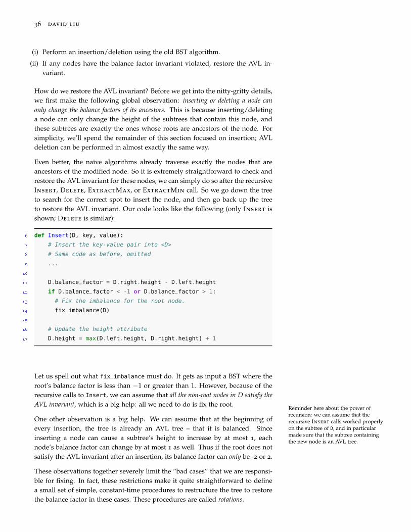
Even better, the naïve algorithms already traverse exactly the nodes that areancestors of the modified node. So it is extremely straightforward to check andrestore the AVL invariant for these nodes; we can simply do so after the recursiveInsert, Delete, ExtractMax, or ExtractMin call. So we go down the treeto search for the correct spot to insert the node, and then go back up the treeto restore the AVL invariant. Our code looks like the following (only Insert isshown; Delete is similar):


7 # Insert the key-value pair into <D>

8 # Same code as before, omitted

9 ...

10

11 D.balance_factor = D.right.height - D.left.height

12 if D.balance_factor < -1 or D.balance_factor > 1:

13 # Fix the imbalance for the root node.

14 fix_imbalance(D)

15

16 # Update the height attribute

17 D.height = max(D.left.height, D.right.height) + 1

Let us spell out what fix_imbalance must do. It gets as input a BST where theroot’s balance factor is less than −1 or greater than 1. However, because of therecursive calls to Insert, we can assume that all the non-root nodes in D satisfy theAVL invariant, which is a big help: all we need to do is fix the root.

Reminder here about the power ofrecursion: we can assume that therecursive Insert calls worked properlyon the subtree of D, and in particularmade sure that the subtree containingthe new node is an AVL tree.

One other observation is a big help. We can assume that at the beginning ofevery insertion, the tree is already an AVL tree – that it is balanced. Sinceinserting a node can cause a subtree’s height to increase by at most 1, eachnode’s balance factor can change by at most 1 as well. Thus if the root does notsatisfy the AVL invariant after an insertion, its balance factor can only be -2 or 2.

These observations together severely limit the “bad cases” that we are responsi-ble for fixing. In fact, these restrictions make it quite straightforward to definea small set of simple, constant-time procedures to restructure the tree to restorethe balance factor in these cases. These procedures are called rotations.


Right rotation

Rotations are best explained through pictures. In the top diagram, variables xand y are keys, while the triangles A, B, and C represent arbitrary subtrees (thatcould consist of many nodes). We assume that all the nodes except y satisfy theAVL invariant, and that the balance factor of y is -2.

This means that ys left subtree must have height 2 greater than its right subtree,and so A.height = C.height + 1 or B.height = C.height + 1. We will first considerthe case A.height = C.height + 1.

y

x C

A B

x

A y

B CIn this case, we can perform a right rotation to make x the new root, movingaround the three subtrees and y as in the second diagram to preserve the BSTproperty. It is worth checking carefully that this rotation does indeed restore theinvariant.

Lemma 3.1 (Correctness of right rotation). Let x, y, A, B, and C be defined as inthe margin figure. Assume that this tree is a binary search tree, and that x andevery node in A, B, and C satisfy the balance factor invariant. Also assume thatA.height = C.height + 1, and y has a balance factor of -2.

Then applying a right rotation to the tree results in an AVL tree, and in particu-lar, x and y satisfy the AVL invariant.

Proof. First, observe that whether or not a node satisfies the balance factor in-variant only depends on its descendants. Then, since the right rotation doesn’tchange the internal structure of A, B, and C, all the nodes in these subtrees stillsatisfy the AVL invariant after the rotation. So we only need to show that both

This is the power of having a localproperty like the balance factor invari-ant. Even though A, B, and C movearound, their contents don’t change.

x and y satisfy the invariant.

• Node y. The new balance factor of y is C.height − B.height. Since x origi-nally satisfied the balance factor, we know that B.height ≥ A.height − 1 =

C.height. Moreover, since y originally had a balance factor of −2, we knowthat B.height ≤ C.height + 1. So B.height = C.height or B.height = C.height +1, and the balance factor is either -1 or 0.

• Node x. The new balance factor of x is (1+max(B.height, C.height))−A.height.Our assumption tells us that A.height = C.height+ 1, and as we just observed,either B.height = C.height or B.height = C.height + 1, so the balance factor ofx is 0 or 1.

Left-right rotation

What about the case when B.height = C.height + 1 and A.height = C.height?Well, before we get ahead of ourselves, let’s think about what would happen ifwe just applied the same right rotation as before.

38 david liu

The diagram looks exactly the same, and in fact the AVL invariant for y stillholds. The problem is now the relationship between A.height and B.height: be-cause A.height = C.height = B.height − 1, this rotation would leave x with abalance factor of 2. Not good.

Since in this case B is “too tall,” we will break it down further and move itssubtrees separately. Keep in mind that we’re still assuming the AVL invariant issatisfied for every node except the root y.

y

x C

A z

D E

y

z C

x E

A D

z

x y

A D E C

By our assumption, A.height = B.height− 1, and so both D and E’s heights areeither A.height or A.height− 1. Now we can first perform a left rotation rootedat x, which is symmetric to the right rotation we saw above, except the root’sright child becomes the new root.

This brings us to the situation we had in the first case, where the left subtree of zis at least as tall as the right subtree of z. So we do the same thing and performa right rotation rooted at y. Note that we’re treating the entire subtree rooted atx as one component here.

Given that we now have two rotations to reason about instead of one, a formalproof of correctness is quite helpful.

Lemma 3.2. Let A, C, D, E, x, y, and z be defined as in the diagram. Assumethat x, z, and every node in A, C, D, E satisfy the AVL invariant. Furthermore,assume the following restrictions on heights, which cause the balance factor ofy to be -2, and for the D− z− E subtree (“B”) to have height C.height + 1.

(i) A.height = C.height

(ii) D.height ≤ C.height and E.height ≤ C.height, and one of them is equal toC.height.

Then after performing a left rotation at x, then a right rotation at y, the resultingtree is an AVL tree. This combined operation is sometimes called a left-rightdouble rotation.

Proof. As before, because the subtrees A, C, D, and E don’t change their internalcomposition, all their nodes still satisfy the AVL invariant after the transforma-tion. We need to check the balance factor for x, y, and z:

• Node x: by assumption (ii) and the fact that z originally satisfied the AVLinvariant, D.height = C.height or D.height = C.height− 1. So then the balancefactor of x is D.height− A.height, which is either 0 or -1. (By (i), A.height =C.height.)

• Node y: as in the above argument, either E.height = C.height or E.height =

C.height − 1. Then the balance factor of y is C.height − E.height, which iseither 0 or 1.

• Node z: since D.height ≤ A.height and E.height ≤ C.height, the balance factorof z is equal to (C.height + 1)− (A.height + 1). By assumption (i), A.height =C.height, so the balance factor of z is 0.


We leave it as an exercise to think about the cases where the right subtree’s heightis 2 more than the left subtree’s. The arguments are symmetric; the two relevantrotations are “left” and “right-left” rotations.

AVL tree implementation

We now have a strong lemma telling us that we can rearrange the tree in constanttime to restore the balanced property. This is great for our insertion and deletionalgorithms, which only ever change one node. Here is our full AVL tree Insert

algorithm:

You’ll notice that we’ve deliberatelyleft some details to the exercises. Inparticular, we want you to think aboutthe symmetric actions for detecting andfixing an imbalance.


7 # Insert the key-value pair into <D>

8 # Same code as before, omitted

9 ...

10

11 D.balance_factor = D.right.height - D.left.height

12 if D.balance_factor < -1 or D.balance_factor > 1:

13 # Fix the imbalance for the root node.

14 fix_imbalance(D)

15

16 # Update the height attribute

17 D.height = max(D.left.height, D.right.height) + 1

18

19

20 def fix_imbalance(D):

21 # Check balance factor and perform rotations

22 if D.balance_factor == -2:

23 if D.left.left.height == D.right.height + 1:

24 right_rotate(D)

25 else: # D.left.right.height == D.right.height + 1

26 left_rotate(D.left)

27 right_rotate(D)

28 elif D.balance_factor == 2:

29 # left as an exercise; symmetric to above case

30 ...

31

32

33 def right_rotate(D):

34 # Using some temporary variables to match up with the diagram

35 y = D.root

36 x = D.left.root

37 A = D.left.left

38 B = D.left.right

39 C = D.right

40 david liu

40

41 D.root = x

42 D.left = A

43 # Assume access to constructor AVLTree(root, left, right)

44 D.right = AVLTree(y, B, C)

45

46

47 def left_rotate(D):

48 # Left as an exercise

Theorem 3.3 (AVL Tree Correctness). The above AVL Tree insertion algorithmis correct. That is, it results in a binary tree that satisfies the binary search treeproperty and is balanced, with one extra node added, and with the height andbalance_factor attributes set properly.

Proof. Since insertion starts with the naïve algorithm, we know that it correctlychanges the contents of the tree. We need only to check that fix_imbalance

results in a balanced BST.

Right before fix_imbalance is called in either function, we know that D stillsatisfies the BST property, and that its subtrees are AVL trees (since we assumethat the recursive calls correctly restore this property). Moreover, because atmost one node has changed in the BST, the balance factor of the root is between-2 and 2.

The correctness of fix_imbalance when the root’s balance factor is -2 is directlyimplied by the previous two lemmas. The other case is symmetric, and was leftas an exercise. Then we are done, since after fix_imbalance returns, the tree isan AVL tree – all its nodes satisfy the AVL invariant.

Analysis of AVL Algorithms

In the preceding sections, we put in quite a bit of effort in ensuring that the AVLinvariant is preserved for every node in the tree. Now, it is time to reap thebenefits of this additional restriction on the structure of the tree in our runningtime analysis of the modified Insert and Delete algorithms.

First, a simple lemma that should look familiar, as it is the basis of most recursivetree algorithm analyses.

Lemma 3.4. The worst-case running time of AVL tree insertion and deletion isO(h), the same as for the naïve insertion and deletion algorithms.

Don’t forget that we’ve only proveda O(h) upper bound in these notes –you’re responsible for proving a lowerbound yourself!Proof. We simply observe that the new implementation consists of the old one,

plus the new updates of height and balance_factor attributes, and at most tworotations. This adds a constant-time overhead per recursive call, and as before,there are O(h) recursive calls made. So the total running time is still O(h).


So far, the analysis is exactly the same as for naïve BSTs. Here is where wediverge to success. As we observed at the beginning of this section, BSTs can beextremely imbalanced, and have height equal to the number of nodes in the tree.This is obviously not true for AVL trees, which cannot have all their nodes on(say) the left subtree. But AVL trees are not perfectly balanced, either, since eachnode’s two subtree heights can differ by 1. So the question is, is restricting thebalance factor for each node to the range −1, 0, 1 good enough to get a strongbound on the height of the AVL tree? The answer is a satisfying yes.

Lemma 3.5 (AVL Tree Height). An AVL tree with n nodes has height at most1.441 log n (for large enough n).

Proof. It turns out to be easier to answer a question that is inverse to the state-ment in the theorem: what is N(h), the minimum number of nodes in an AVL treeof height h? Our goal is to get a tight bound (or exact formula) for N(h). Someplaying around quickly yields the following small values: N(0) = 0, N(1) = 1,N(2) = 2, N(3) = 4, N(4) = 7.

Not much of a pattern so far, though drawing pictures is suggestive: an AVLtree of height h with minimum size must have a subtree that is an AVL tree ofheight h− 1, and another subtree that is an AVL tree of height h− 2, and both ofits subtrees must have minimum size. Here we’re implicitly using the fact thatbeing balanced, and hence an AVL tree, is a recursive property: the subtrees ofan AVL tree are themselves AVL trees. This gives the following recurrence:

N(h) =

0, h = 0

1, h = 1

N(h− 1) + N(h− 2) + 1, h ≥ 2

This looks almost, but not quite, the same as the Fibonacci sequence. A bit oftrial-and-error or more sophisticated techniques for solving recurrences (beyondthe scope of this course) reveal that N(h) = fh+2 − 1, where fi is the i-th Fi-bonacci number. Since we do have a closed form expression for the Fibonaccinumbers in terms of the golden ratio ϕ = 1+

√5

2 , we get the following bound onN(h):

N(h) > fh

>1√5

ϕh − 1

Recall now the definition of N(h): the minimum number of nodes in an AVLtree of height h. So then if we have n nodes in an AVL tree of height h, we knowthat

42 david liu

N(h) ≤ n1√5

ϕh − 1 ≤ n

1√5

ϕh ≤ n + 1

logϕ

(1√5

ϕh)≤ logϕ(n + 1)

logϕ

(1√5

)+ h ≤ logϕ(n + 1)

h ≤ logϕ(n + 1)− logϕ

(1√5

)h ≤ 1.4405 log(n + 1)− logϕ

(1√5

)h ≤ 1.4405 log(n + 1) + 1.68

Putting the previous two lemmas together, we can conclude that AVL insertion,deletion, and search all have logarithmic running time in the worst-case.

Theorem 3.6 (AVL Tree Runtime). AVL tree insertion, deletion, and search haveworst-case running time Θ(log n), where n is the number of nodes in the tree.

Exercise Break!

3.7 Show that you can use an AVL tree to implement a priority queue. What isan upper bound on the worst-case running time of the three priority queueoperations in this case?

4 Dictionaries, Round Two: Hash Tables

We now look at a completely different approach for implementing dictionaries.To get warmed up, consider the following scenario: all of the key-value pairswe wish to store have keys that are numbers 0 through K − 1. In this case,we can store these pairs inside an array of length K, and achieve constant timesearch, insertion, and deletion simply by storing each value at the array indexcorresponding to its key!

This technique is known as direct addressing, and works well when the numberof possible keys (and hence total number of pairs) is small. However, arrayaddressing is only constant time if the entire array has been allocated in memory.Thus as K grows larger, even if the running time of the dictionary operationsstays constant, the space required grows linearly in K. In this chapter, we will

This size constraint is infeasible inmany real-world applications of dictio-naries.

study a generalized version of direct addressing known as hashing, which allowsus to store key-value pairs when the keys aren’t necessarily numbers, and usingmuch less space than the number of all possible keys.

Hash functions

Let U represent the set of all possible keys we would like to store. In general, wedo not restrict ourselves to just numeric keys, and so U might be a set of strings,floating-point numbers, or other custom data types that we define based on ourapplication. Like direct addressing, we wish to store these keys in an array, buthere we’ll let the size of the array be a separate variable m. We won’t assumeanything about the relationship between m and |U| right now, though you mightalready have some ideas about that.

Definition 4.1 (hash function, hash table). A hash function is a function h :U → 0, 1, . . . , m− 1. You should think of this as a function that takes a keyand computes the array slot where the key is to be placed.

A hash table is a data structure containing an array of length m and a hashfunction.

6 def Search(hash_table, key):

7 hash = h(key)

8 return hash_table[hash]

9

44 david liu

10 def Insert(hash_table, key, value):

11 hash = h(key)

12 hash_table[hash] = value

13

14 def Delete(hash_table, key):

15 hash = h(key)

16 hash_table[hash] = None

Of course, this is not the end of the story. Even though this implementationis certainly efficient – all three operations run in Θ(1) time – it actually is notguaranteed to be correct.

Remember that we have not made any assumptions about the relationship be-tween m, the size of the hash table, and |U|, the total possible number of keys;nor have we said anything about what h actually does. Our current implemen-tation makes the assumption that there are no collisions in the hash function; i.e.,that each key gets mapped to a unique array slot. Consider what happens whenyou try to use the above algorithm to insert two key-value pairs whose hashedkeys are the same index i: the first value is stored at index i, but then the secondvalue overwrites it.

Now, if m ≥ |U|, i.e, there are at least as many array slots as possible keys, thenthere always exists a hash function h which has no collisions. Such hash func-tions are called perfect hash functions, earning the superlative name becausethey enable the above naive hash table implementation to be correct. However,

Of course, even when we know that aperfect hash function exists for a givenU and m, it is sometimes non-trivial tofind and compute it. Consider the casewhen U is a set of 10 000 names – canyou efficiently implement a perfect hashfunction without storing a sorted list ofthe names?

this assumption is often not realistic, as we typically expect the number of pos-sible keys to be extremely large, and the array to not take up too much space.More concretely, if m < |U|, then at least one collision is guaranteed to occur,causing the above implementation to fail. The remainder of this chapter will bedevoted to discussing two strategies for handling collisions.

Closed addressing (“chaining”)

With closed addressing, each array element no longer stores a value associatedthis approach is also called “chaining”

with a particular key, but rather a pointer to a linked list of key-value pairs. Thus,collisions are sidestepped completely by simply inserting both the key and valueinto the linked list at the appropriate array index. Search and deletion are just

Why is it necessary to store both thekey and the value?slightly more complex, requiring a traversal of the linked list to find the correct

key-value pair.


6 hash = h(key)

7 linked_list = hash_table[hash]

8 if linked_list contains key:

9 return corresponding value from linked_list

10 else:


11 return None

12


14 hash = h(key)


16 insert key, value at the head of linked_list

17

18 def Delete(hash_table, key):

19 hash = h(key)


21 delete key from linked_list

This implementation maintains the invariant that for every key k stored in thetable, it must appear in the linked list at position h(k). From this observation,we can see that these algorithms are correct. In addition, these algorithms onlyconsider the linked list at one particular array index, saving lots of time.

Or perhaps not. What if all of the keys get mapped to the same index? In thiscase, the worst case of search and deletion reduces to the worst-case search anddeletion from a linked list, which is Θ(n), where n is the number of pairs storedin the hash table. Can we simply pick a hash function that guarantees that thisextreme case won’t happen? Not if we allow the set of keys to be much largerthan the size of the array: for any hash function h, there exists an index i suchthat at least |U|/m keys get mapped to i by h.

This type of counting argument is ex-tremely common in algorithm analysis.If you have a set of numbers whoseaverage is x, then one of the numbersmust have value ≥ x.

So while the worst-case running time for Insert is Θ(1),, the worst case per-

Insertions happen at the front of thelinked list

formance for Search and Delete seems very bad: no better than simply usinga linked list, and much worse than the AVL trees we saw in the previous sec-tion. However, it turns out that if we pick good hash functions, hash tables withclosed addressing are much better than both of these data structures on average.

Average-case analysis for closed addressing

We will focus on analysing the Search algorithm, whose running time of coursedepends on the lengths of the linked lists in the hash table. Remember that

Delete is basically the same.whenever we want to talk about average case, we need to define a distributionof inputs for the operation. We’ll assume here that all possible keys are equallylikely to be searched for; in other words, we’ll use the uniform distribution onU, and assume n random keys are already contained in the hash table.

However, because the lengths of the linked lists depend on the number of col-lisions in our hash function, just knowing the key distribution isn’t enough –for all we know, our hash function could map all keys to the same index! Sowe will make an additional assumption known as the simple uniform hashingassumption, which is that our hash function h satisfies the property that for all0 ≤ i < m, the probability that h(k) = i is 1

m , when k is chosen uniformly atrandom from U. That is, choosing a random key doesn’t favour one particu-

46 david liu

lar index over any other. We will measure running time here as the number ofkeys compared against the search input, plus the time for computing the hashfunction.

First, assume that the key k being searched for is not in the hash table. In thiscase, the algorithm first computes h(k), and then must traverse the entire linkedlist stored at index h(k). We’ll assume that the first step takes constant time,

More on this laterand we know that the second step takes time proportional to the length of thelinked list at index h(k). Let T be the running time of Search on input keyk. Then T = 1+ the length of the linked list stored at h(k), which is equalto the number of the n keys that hash to that particular index. We let L be arandom variable representing the number of keys hashed to h(k). So, T = 1+ L,and E[T] = 1 + E[L]. But, by the simple uniform hashing assumption, theprobability that each of the n randomly chosen keys already in the hash tablehave a hash value of h(k) is 1

m , and so E[L] = nm .

This is the well-known expected valuefor a hypergeometric distribution.

The average number of keys checked by Search when the key is not in thehash table is therefore 1 + n

m . The average-case running time is then Θ(1 + nm ).

Remember what these variables mean: n is the number of keys already storedin the hash table, and m is the number of spots in the array. This running timetells us that if the number of keys in the hash table is any constant multiple ofthe size of the array, then doing a search when the key is not in the hash table isa constant-time operation on average.

What about when the search is successful, i.e., when we search for a key that isalready in the hash table? Consider searching for ki, the i-th key inserted intothe hash table. How many keys are checked during this search? Since itemsare inserted at the front of the linked list, the number of keys searched is equalto the number of keys inserted after ki into the same index as ki, plus one forexamining ki itself. Since n− i keys are inserted after ki, by the simple uniformhashing assumption the expected number of keys inserted into h(ki) after ki isn−im . So then to compute the average running time, we add the cost of computing

the hash function (just 1 step) plus the average of searching for each ki:

E[T] = 1 +1n

n

∑i=1

expected number of keys visited by search for ki

= 1 +1n

n

∑i=1

(1 +

n− im

)= 2 +

1n

n

∑i=1

nm− 1

n

n

∑i=1

im

= 2 +nm− 1

n· n(n + 1)

2m

= 2 +nm− n + 1

2m

= 2 +n

2m− 1

2m

= Θ(

1 +nm

)The average-case running time for Delete is the same, since once a key has


been found in an array, it is only a constant-time step to remove that node fromthe linked list.

Because the ratio nm between the number of keys stored and the number of spots

in the array comes up frequently in hashing analysis, we give it a special name.

Definition 4.2 (load factor). The load factor of a hash table is the ratio of thenumber of keys stored to the size of the table. We use the notation α = n

m , wheren is the number of keys, and m the number of slots.

So we can say that the average-case running time of Search and Delete areΘ(1 + α).

Exercise Break!

4.1 Suppose that we use an AVL tree instead of a linked list to store the key-valuepairs that are hashed to the same index.

(a) What is the worst-case running time of a search when the hash table has nkey-value pairs?

(b) What is the average-case running time of an unsuccessful search when thehash table has n key-value pairs?

Open addressing

The other strategy used to resolve collisions is to require each array element tocontain only one key, but to allow keys to be mapped to alternate indices whentheir original spot is already occupied. This saves the space overhead requiredfor storing extra references in the linked lists of closed addressing, but the cost isthat the load factor α must always be less than 1, i.e., the number of keys storedin the hash table cannot exceed the length of the array.

In this type of hashing, we have a parameterized hash function h that takes twoarguments, a key and a positive integer. The “first” hash value for a key k is

h : U ×N→ 0, . . . , m− 1h(k, 0), and if this spot is occupied, the next index chosen is h(k, 1), and thenh(k, 2), etc.

For simplicity, we have omitted abounds check i < m. This would benecessary in practice to ensure thatthis code does not enter into an infiniteloop.


6 i = 0

7 while hash_table[h(key, i)] is not None:

8 i = i + 1

9

10 hash_table[h(key, i)].key = key

11 hash_table[h(key, i)].value = value

48 david liu

Searching for an item requires examining not just one spot, but many spots.Essentially, when searching for a key k, we visit the same sequence of indicesh(k, 0), h(k, 1), etc. until either we find the key, or reach a None value.


15 i = 0

16 while hash_table[h(key, i)] is not None and hash_table[h(key, i)].key != key:

17 i = i + 1

18

19 if hash_table[h(key, i)].key == key:

20 return hash_table[h(key, i)].value

21 else:

22 return None

Deletion seems straightforward – simply search for the given key, then replacethe item stored in the array with None, right? Not exactly. Suppose we inserta key k into the hash table, but the spot h(k, 0) is occupied, and so this key isstored at index h(k, 1) instead. Then suppose we delete the pair that was storedat h(k, 0). Any subsequent search for k will start at h(k, 0), find it empty, and soreturn None, not bothering to continue checking h(k, 1).

So instead, after we delete an item, we replace it with a special value Deleted,rather than simply None. This way, the Search algorithm will not halt when itreaches an index that belonged to a deleted key.

We leave it as an exercise to modify theInsert algorithm so that it stores keysin Deleted positions as well.25 def Delete(hash_table, key):

26 i = 0

27 while hash_table[h(key, i)] is not None and hash_table[h(key, i)].key != key:

28 i = i + 1

29

30 if hash_table[h(key, i)].key == key:

31 hash_table[h(key, i)] = Deleted

It remains to discuss how to implement different parameterized hash functionsand to study the properties of the probe sequences [h(k, 0), h(k, 1), . . . ] generatedby these different strategies. After all, since all three dictionary operations re-quire traversing one of these probe sequences until reaching an empty spot, anatural question to ask is how the probe sequences for different keys overlapwith each other, and how these overlaps affect the efficiency of open addressing.

Linear probing

The simplest implementation of open addressing is to start at a given hash value,and then keep adding some fixed offset to the index until an empty spot is found.


Definition 4.3 (Linear probing). Given a hash function hash : U → 0, . . . ,m− 1 and number b ∈ 1, . . . , m− 1, we can define the parameterized hashfunction h for linear probing as follows:

Recall that (mod m) takes the remain-der when divided by m.h(k, i) = hash(k) + bi (mod m).

The corresponding linear probing sequence for key k is hash(k, 0), hash(k, 1),hash(k, 2), . . .

When d = 1, the probe sequence is simply hash(k), hash(k) + 1, . . .

Unfortunately, this strategy suffers from a fundamental problem of clustering,in which contiguous blocks of occupied locations are created, causing furtherinsertions of keys into any of these locations to take a long time. For example,suppose d = 1, and that three keys are inserted, all with the hash value 10.These will occupy indices 10, 11, and 12 in the hash table. But now any new keywith hash value 11 will require 2 spots to be checked and rejected because theyare full. The collision-handling for 10 has now ensured that hash values 11 and12 will also have collisions, increasing the runtime for any operation that visitsthese indices. Moreover, the effect is cumulative: a collision with any index in acluster causes an extra element to be added at the end of the cluster, growing itin size by one. You’ll study the effects of clustering more precisely in an exercise.

Quadratic probing

The main problem with linear probing is that the hash values in the middle of acluster will follow the exact same search pattern as a hash value at the beginningof the cluster. As such, more and more keys are absorbed into this long searchpattern as clusters grow. We can solve this problem using quadratic probing,which causes the offset between consecutive indices in the probe sequence toincrease as the probe sequence is visited.

Definition 4.4 (Quadratic probing). Given a hash function hash : U → 0, . . . , m−1 and numbers b, c ∈ 0, . . . , m − 1, we can define the parameterized hashfunction h for quadratic probing as follows:

h(k, i) = hash(k) + bi + ci2 (mod m).

Even if a key’s hash value is in the middle of a cluster, it is able to “escape”the cluster much more quickly than using linear probing. However, a form ofclustering still occurs: if many items have the same initial hash value, they stillfollow the exact same probe sequence. For example, if four keys are hashedto the same index, the fourth key inserted must examine (and pass) the threeindices occupied by the first three keys.

Double hashing

To resolve this problem – a collision in the original hash function causing identi-cal probe sequences – we change how the offset is calculated so that it dependson the key being hashed in a particularly clever way.

50 david liu

Definition 4.5 (Double hashing). Given two hash functions hash1, hash2 : U →0, . . . , m− 1, we can define the parameterized hash function for double hash-ing h as follows:

h(k, i) = hash1(k) + i · hash2(k) (mod m).

While both linear and quadratic probing have at most m different probe se-quences (one for each distinct starting index), double hashing has at most m2

different probe sequences, one for each pair of values (hash1(k), hash2(k)). Un-der such a scheme, it is far less likely for large clusters to form: not only wouldkeys have to have the same initial hash value (using hash1), but they would alsohave to have the same offset (using hash2).

Running time of open addressing

To round out this chapter, we’ll briefly discuss some of the performance charac-teristics of open addressing. First, we observe that there are m! possible probesequences (i.e., the order in which hash table indices are visited). A typical sim-plifying assumption is that the probability of getting any one of these sequencesis 1/m!, which is not true for any of the probe sequences studied here – evendouble hashing has only m2 possible sequences – but can be a useful approxi-mation.

However, under this assumption, the average number of indices searched of allthree dictionary operations is at most 1

1−α . So for example, if the table is 90%full (so α = 0.9), the average number of indices searched would be just 10, whichisn’t bad at all!

Exercise Break!

4.2 Suppose we use linear probing with d = 1, and our hash table has n keysstored in the array indices 0 through n− 1.

(a) What is the maximum number of array indices checked when a new key(distinct from the ones already stored) is searched for in this hash table?

(b) What is the probability that this maximum number of array indices occurs?Use the simple uniform hashing assumption.

(c) What is the average running time of Search for this array?

5 Randomized Algorithms

So far, when we have used probability theory to help analyse our algorithms wehave always done so in the context of average-case analysis: define a probabilitydistribution over the set of possible inputs of a fixed size, and then calculate theexpected running time of the algorithm over this set of inputs.

This type of analysis is a way of refining our understanding of how quickly analgorithm runs, beyond simply the worst and best possible inputs, we look atthe spread (or distribution) of running times across all different inputs. It allowsus to say things like “Quicksort may have a worst-case running time of Θ(n2),but on average its performance is Θ(n log n), which is the same as mergesort.”

However, average-case analysis has one important limitation: the importance ofthe asymptotic bound is directly correlated with the “plausibility” of the prob-ability distribution used to perform the analysis. We can say, for example, thatthe average running time of quicksort is Θ(n log n) when the input is a random,uniformly-chosen permutation of n items; but if the input is instead randomlychosen among only the permutations which have almost all items sorted, the“average” running time might be Θ(n2). We might assume that the keys in-

This assumes naïve quicksort, whichchooses the first element as the pivot.serted into a hash table are equally likely to be hashed to any of the m array

spots, but if they’re all hashed to the same spot, searching for keys not alreadyin the hash table will always take Θ(n) time.

In practice, an algorithm can have an adversarial relationship with the entityfeeding it inputs. Not only is there no guarantee that the inputs will have adistribution close to the one we used in our analysis; a malicious user could con-ceivably hand-pick a series of inputs designed to realize the worst-case runningtime. That the algorithm has good average-case performance means nothing inthe face of an onslaught of particularly bad inputs.

In this chapter, we will discuss one particularly powerful algorithm design tech-nique which can (sometimes) be used to defend against this problem. Ratherthan assume the randomness exists external to the algorithm in the choice ofinputs, this technique makes no assumptions about the input whatsoever, butinstead moves the randomness to be inside the algorithm itself. The key ideais to allow our algorithms to make random choices, a departure from the deter-ministic algorithms — ones that must follow a fixed sequence of steps — thatwe have studied so far. Such algorithms, which make random choices as part oftheir natural execution, are known as randomized algorithms.

52 david liu

Randomized quicksort

Let us return to quicksort from our first chapter, which we know has poorworst-case performance on pre-sorted lists. Because our implementation alwayschooses the first list element as the pivot, a pre-sorted list always results inmaximally uneven partition sizes. We were able to “fix” this problem in ouraverage-case analysis with the insight that in a random permutation, any of then input numbers is equally likely to be chosen as a pivot in any of the recursivecalls to quicksort.

You’ll recall our argument was a tadmore subtle and relied on indicatorvariables, but this idea that the pivotwas equally likely to be any numberdid play a central role.

So if we allow our algorithm to make random choices, we can turn any inputinto a “random” input simply by preprocessing it, and then applying the regularquicksort function:

1 def randomized_quicksort(A):

2 randomly permute A

3 quicksort(A)

Huh, this is so simple it almost feels like cheating. The only difference is theapplication of a random permutation to the input. The correctness of this al-gorithm is clear: because permuting a list doesn’t change its contents, the exactsame items will be sorted, so the output will be the same. What is more inter-

This isn’t entirely true if the list con-tains duplicates, but there are ways offixing this if we need to.

esting is talking about the running time of this algorithm.

One important point to note is that for randomized algorithms, the behaviourof the algorithm depends not only on its input, but also the random choices it makes.Thus running a randomized algorithm multiple times on the same input canlead to different behaviours on each run. In the case of randomized quicksort,we know that the result — A is sorted — is always the same. What can changeis its running time; after all, it is possible to get as input a “good” input for theoriginal quicksort (sorts in Θ(n log n) time), but then after applying the randompermutation the list becomes sorted, which is the worst input for quicksort.

In other words, randomly applying a permutation to the input list can cause therunning time to increase, decrease, or stay roughly the same. So how do wedraw conclusions about the running time of randomized quicksort if we can’teven be certain how long it takes on a single input? Probability, of course!

More precisely, for a fixed input A to randomized quicksort with length n, wecan define the random variable TA to be the running time of the algorithm.The main difference between this random variable and the T we used in theaverage-case analysis of Chapter 1 is that now we are considering the proba-bility distribution that the algorithm uses to make its random choices, and nota probability distribution over inputs. In the case of randomized quicksort, wewould say that the TA random variable has as its probability space the set of ran-dom permutations of 1, . . . , n that the randomized_quicksort algorithm couldpick from in its first step.

With this random variable defined, we can now talk about the expected running


time of randomized quicksort on the input A, E[TA]. First, while we won’tprove it here, it is possible to randomly permute A in O(n) time. Applying

See Section 5.3 of CLRS for details.a random permutation on A results in the standard quicksort running on arandom permutation of 1, . . . , n as its input, and so the analysis from Chapter1 applies, and E[TA] = Θ(n log n).

Warning: students often confuse this type of analysis with the average-case anal-ysis we did earlier in the course. For average-case analysis, we have a completelydeterministic algorithm and a probability distribution over a set of inputs, andare calculating the expected running time across this set of inputs. For the anal-ysis in the present chapter, we have a randomized algorithm and a single in-put, and are calculating the expected running time across the possible randomchoices made by the algorithm itself.

You can think about average-caseanalysis as putting the randomnessexternal to the algorithm, and random-ized algorithm analysis as keeping therandomness internal to the algorithm.

The work we have done so far is just for one particular input. Let us extend thisnow to be able to say something about the overall running time of the algorithm.We define the worst-case expected running time of a randomized algorithm tobe a function

ET(n) = maxE[Tx] | x is an input of size n.

For randomized quicksort, all lists of size n have the same asymptotic expectedrunning time, and so we conclude that randomized quicksort has a worst-caseexpected running time of Θ(n log n).

You might hear the phrase “worst-case expected” and think this is a bit vague:it’s not the “absolute” maximum running time, or even an “average” maximum.So what is this really telling us? The right way to think about worst-case ex-pected running time is from the perspective of a malicious user who is tryingto feed our algorithm bad inputs. With regular quicksort, it is possible to givethe algorithm an input for which the running time is guaranteed to be Θ(n2).However, this is not the case for randomized quicksort. Here, no matter whatinput the user picks, if the algorithm is run many times on this input, the aver-age running time will be Θ(n log n). Individual runs of randomized quicksortmight take longer, but in the long run our adversary can’t make our algorithmtake more than Θ(n log n) per execution.

Universal Hashing

Now, let us turn to a well-known example of a randomized algorithm: universalhashing. Recall that the simple uniform hashing assumption from the previouschapter says that for any array index 0 ≤ i < m, the probability of choosing akey that hashes to i is 1

m . This assumption made the analysis tractable for us,and in particular ensured a Θ(1 + α) average-case running time for the hashtable operations. But as we observed, for any hash function we choose, a simplecounting argument tells us that at least |U|/m keys must be hashed to the sameindex. So if any subset of size n of these keys is inserted, any search for adifferent key that hashes to this same index will take Θ(n) time.

To cause this worst-case behaviour in practice, a malicious user would study the

54 david liu

hash function used and determine such a set of colliding keys. You might betempted, then, to keep your hash function a secret so that no one can figure outthese collisions. But a reliance on such an approach only goes so far as how ableyou (and your colleagues) are in keeping this secret.

But let us take from this the insight that a malicious user needs to know whichhash function is being used in order to purposefully generate large numbers ofcollisions. Rather than keep the hash function a secret, we simply use a set ofhash functions, and allow our algorithm to pick randomly which one to actuallyuse, without making its choice public. To “normal” users, the hash table behavesexactly as expected, regardless of which hash function is used. In other words,the interface of the hash table has not changed. But even if a malicious userknows the whole set of hash functions, she does not know which one is actuallybeing used by the hash table, and in principle cannot determine how to generatecollisions.

Of course, if we picked a poor set of hash functions, it might be possible thateach one has a huge number of collisions, or that the same keys collide for allor most of the functions. So we certainly need some restriction on the hashfunctions that can go into this set; we make this idea precise in the followingdefinition.

Definition 5.1 (Universal hash family). Let U be a set of keys, and m ∈ Z+ bethe size of the hash table. Let H be a set of hash functions, where each h ∈ His a function h : U → 0, . . . , m− 1. We call H a universal hash family if andonly if for all pairs of distinct keys k1, k2 ∈ U,

Note that the probability space is nowthe choice of hash functions, and notchoice of keys. This inequality must betrue for every pair of keys!

Prh∈H[h(k1) = h(k2)] ≤1m

.

Our algorithm is now quite simple. When a new hash table is created, it picks ahash function uniformly at random from a universal hash family, and uses thisto do its hashing. This type of hashing is called universal hashing, and is arandomized implementation of hashing commonly used in practice.

Analysis of universal hashing

Consider a universal hashing scheme that uses closed addressing (chaining). Wewill consider the worst-case expected running time of an unsuccessful search for akey k in a hash table storing n keys. Note that this analysis is related to, butdistinct from, the analysis we did in the previous chapter. Both are probabilistic,of course, but their probability spaces are different (choosing keys vs. choosinghash functions), and the probability assumptions we are allowed to make arealso different, albeit quite similar.

Let h ∈ H be the hash function used by the hash table (chosen uniformly atrandom). We want to consider how many of the n keys already in the hash tablewere inserted into the index h(k), since these keys are the ones that must beexamined in a search for k.

For each inserted key ki, let Xi be the indicator random variable that is 1 ifh(ki) = h(k), and 0 otherwise. We want to compute the expected sum of these


random variables, which we can do nicely using the techniques that we’ve seenbefore. Again, keep in mind that expected values and probabilities are overchoice of hash function h, not over choice of keys.

E

[n

∑i=1

Xi

]=

n

∑i=1

E[Xi]

=n

∑i=1

Pr[h(ki) = h(k)]

≤n

∑i=1

1m

(universal hash family)

=nm

Note that we have made no assumptions about the keys in the hash table, norabout k itself: the only property we used was the universal hash family property,which gave us the upper bound on the probability that the two hash values h(ki)

and h(k) were equal. Because this analysis is true for all possible inputs, weconclude that the worst-case expected running time of an unsuccessful searchwith universal hashing is O(1+ α), where the 1 comes from computing the hash

Why didn’t we immediately concludeΘ(1 + α)?value of k, as before. A similar analysis reaches the same asymptotic bound for

a successful search.

Constructing a universal hash family

Let us round off our two-chapter discussion of hashing by looking at one partic-ular construction of a universal hash family.

We assume that U = 0, 1, . . . , 2w − 1 is the set of natural numbers that can bestored in a machine word (so typically w = 32 or w = 64), and that m = 2M is apower of two. For every odd number a, 0 < a < 2w, and number (not necessarilyodd) b, 0 ≤ b < 2w−M, we define the following hash function:

ha,b(k) = (ak + b mod 2w) // 2w−M.

Note that these functions are very easy to implement; the first computationak + b mod 2w is simply unsigned integer arithmetic, and the second operationis a bit shift, taking the M most significant bits.

While we won’t go into the proof here, it turns out that the set of functionsha,b, for the defined ranges on a and b, is a universal hash family.

Exercise Break!

5.1 Prove that the number of hash functions in a universal hash family must be≥ m.

56 david liu

5.2 Consider the hash function

h1,0(k) = (k mod 2w) // 2w−M.

Find a set of inputs of size 2w−M that all have the same hash value.This question underlines the factthat an individual hash function ina universal family still has a lot ofcollisions.

6 Graphs

In this chapter, we will study the graph abstract data type, which is one of themost versatile and fundamental in computer science. You have already studiedtrees, which can be used to model hierarchical data like members of a familyor a classification of living things. Graphs are a generalization of trees thatcan represent arbitrary (binary) relationships between various objects. Some

There are generalizations of graphs thatmodel relationships between more thantwo objects at a time, but we won’t gointo that here.

common examples of graphs in practice are modelling geographic and spatialrelationships; activity between members of a social network; requirements anddependencies in a complex system like the development of a space shuttle. Bythe end of this chapter, you will be able to define the graph ADT and comparedifferent implementations of this data type; and perform and analyse algorithmswhich traverse graphs.

If you go on to take CSC373, youwill build on this knowledge to writeand analyse more complex graphalgorithms.

Fundamental graph definitions

As we hinted at in the introduction, a graph is an abstraction of the concept ofa set of objects and the relationships between them. In the simplest case, wedefine a vertex (also called node) v to be a single object, and an edge to be atuple e = (v1, v2). This is deliberately abstract to be able

to account for a variety of contexts. Forexample, in a social network, you canthink of vertices as people, and edges as“friendships” or “connections.”

Definition 6.1 (graph, undirected/directed). A graph is a tuple of two sets G =

(V, E), where V is a set of vertices, and E is a set of edges on those vertices.

An undirected graph is a graph where order does not matter in the edge tuples:(v1, v2) is equal to (v2, v1). A directed graph is a graph where the tuple order

We think of an edge in an undirectedgraph as being between two vertices, andan edge in a directed graph as beingfrom a source vertex to a target vertex.

does matter; (v1, v2) and (v2, v1) represent different edges. In this chapter, ifneither type of graph is specified, our default will be an undirected graph.

There are two obvious measures of a graph’s size: the number of vertices andthe number of edges. When analysing the running time of graph algorithmslater in this chapter, it will be important to keep in mind how we are defining“size.”

Before moving on, let’s see some pictures to illustrate some simple graphs. Ineach diagram, the vertices are the circles, and the edges are the lines connectingpairs of circles. Vertices can be labelled or unlabelled, depending on the graphcontext.

58 david liu

1 2

3

A B

CDa

bc

de

It is clear that there can be a large variation in the characteristics of graphs: thenumber of edges, how many vertices are connected to each other, how manyedges each vertex has, etc. For our purposes, we will need only a few more

Graph theory is a fascinating branch ofmathematics that studies properties ofgraphs such as these, and ones whichare far more complex.

definitions to describe some simple graph properties.

Definition 6.2 (adjacent, neighbour). Two vertices are adjacent if there is an edgebetween them. In this case, we also say that the two vertices are neighbours.

Definition 6.3 (path, length, distance). A path between vertices u and w is asequence of edges (v0, v1), (v1, v2), . . . , (vk−1, vk), where u = v0 and w = vk, andall the vi are distinct.This follows the English meaning of the term “path,” whereyou start at vertex u, take an edge to get to a new vertex v1, take another edgeto get to another new vertex v2, and keep following edges until arriving at vk.

The length of the path is the number of edges in the path. For example, two ad-jacent vertices are connected by a path of length one, and the previous notationdescribes a path of length k. The distance between two vertices is the length ofthe shortest path between the two vertices. The distance between a vertex anditself is always 0.

Paths are fundamental to graphs because they allow us to take basic relation-ships (edges) and derive more complex ones. Suppose, for example, we arerepresenting all the people of the world, with edges representing “A and B per-sonally know each other.” The famous example from social networks is the ideaof Six Degrees of Separation, which says that on this graph, any two people havea path of length at most 6 between them. Given an arbitrary graph, one mightwonder what the maximum path length is between any two vertices – or evenwhether there is a path at all!

Definition 6.4 (connected). We say that a graph is connected if for every pair ofvertices in the graph, there is a path between them. Otherwise, we say the graphis unconnected.

Implementing graphs

So far, we have discussed graphs as a mathematical abstraction. Our next step isto decide how to represent graphs in a program. To be a bit more concrete, wedefine a Graph ADT with two simple operations: obtaining a list of all verticesin the graph, and checking whether two given vertices are adjacent.

Graph ADT


• Vertices(G): Return a list of all the vertices of G.

• CheckAdjacent(G, u, v): Return whether vertices u and v are adjacent in G.

In this section, we’ll consider two implementations of this ADT: adjacency lists,which generalize our reference-based tree implementations, and an array-basedimplementation known as an adjacency matrix.

Adjacency lists

The first approach is one that should be familiar, because it is essentially whatwe do to implement trees. We use a vertex data type that has a label attribute toidentify the vertex, and a list of references to its neighbours. This latter attributeis known as an adjacency list, from which this implementation gets its name.

In our default undirected case, thismeans that two adjacent vertices eachstore a reference to the other in theirrespective adjacency lists.

Since the vertices keep track of the edge data, a second graph data type storesonly a collection the vertices in the graph. To illustrate this approach, we show

A common implementation stores thevertices in an array, and labels eachvertex with its array index. If we needto support arbitrary unique identifiers,any dictionary implementation (e.g., ahash table) can be used as well.

how one could implement a function that checks whether two vertices in a graphare adjacent. Note that this operation takes labels, and must use them to look upthe corresponding vertices in the graph.

7 def CheckAdjacent(G, i, j):

8 # Access the vertices attribute and perform lookup by labels

9 u = G.vertices[i]

10 v = G.vertices[j]

11 for vertex in u.neighbours:

12 # Note: this assumes labels are unique

13 if vertex.label == v.label:

14 return True

15

16 return False

What is the running time of this algorithm? We assume that looking up the twovertices in graph.vertices takes constant time, so the running time is deter-

This is true if an array is used; we’llleave it as an exercise to think aboutother implementations of this attribute.

mined by the number of loop iterations (since the body of the loop always takesconstant time). What is an upper bound on the number of iterations? Well, ifthere are n vertices in the graph, then u can have at most n− 1 neighbours (ifit has edges going to every other vertex). It might be tempting to say O(n) atthis point. But remember that there are two measures of the size of the graph. Ifthe graph has m edges in total, then m is also an upper bound on the number ofneighbours that u can have. So the number of loop iterations is O(min(m, n)).

For a lower bound, suppose we consider a vertex u that is adjacent to min(m, n−2) vertices, and let v be a vertex that is not adjacent to u. Then performing thisalgorithm will cause all min(m, n− 2) iterations of the loop to occur, resultingin a running time of Ω(min(m, n)).

60 david liu

Adjacency matrices

The previous approach was vertex-focused: each vertex is represented as a sep-arate entity in the program, with edges stored implicitly as the references in theadjacency lists. It is also possible to represent the edges directly in what we callan adjacency matrix. Suppose there are n vertices in some graph, each with alabel between 0 and n − 1. We use an n-by-n two-dimensional boolean array,where the ij-entry of the array is true if there is an edge between vertex i andvertex j.

In the undirected case this matrix issymmetric across its diagonal, while inthe directed case that’s not guaranteed.Using this approach, determining adjacency in a graph runs in constant time,

since it is just an array lookup:

19 def CheckAdjacent(G, i, j):

20 return G.adjacency[i][j]

Implementation space usage

The adjacency matrix approach seems conceptually simpler and easier to imple-ment than the adjacency list approach. However, it does have a relatively highspace cost, since it must use computer memory to store not only the edges, butalso the “non-edges.” This representation must store a full |V|-by-|V| matrix,with a space cost of Θ(|V|2).

In the adjacency list implementation, the graph itself stores an array of sizeΘ(|V|), and each vertex stores its label and references to its neighbours. Wecannot count the number of references for an individual vertex because that canvary dramatically among vertices in an individual graph. But we do have a niceway of calculating the total number of references stored across all vertices.

Definition 6.5 (degree). The degree of a vertex is the number of its neighbours.For a vertex v, we will usually denote its degree by dv.

Lemma 6.1 (handshake lemma). The sum of the degrees of all vertices is equalto twice the number of edges. Or,

∑v∈V

dv = 2|E|.

This lemma gets its name from thereal-life example of meeting people at aparty. Suppose a bunch of people are ata party always shake hands when theymeet someone new. After greetings aredone, if you ask each person how manynew people they met and add them up,the sum is equal to twice the number ofhandshakes that occurred.

Proof. Each edge e = (u, v) is counted twice in the degree sum: once for u, andonce for v.

So this means the total cost of storing the references in our adjacency list datastructure is Θ(|E|), for a total space cost of Θ(|V|+ |E|) (adding a |V| term forstoring the labels). Note that this is the cost for storing all the vertices, not just asingle vertex. Adding up the cost for the graph data structure and all the verticesgives a total space cost of Θ(|V|+ |E|).


At first glance, it may seem that |V|2 and |V|+ |E| are incomparable. However,observe that the maximum number of possible edges is Θ(|V|2), which arises inthe case when every vertex is adjacent to every other vertex. So in asymptoticterms, |V| + |E| = O(|V|2), but this bound is not tight: if there are very few(e.g., O(|V|)) edges then adjacency lists will be much more space efficient thanthe adjacency matrix.

Graph traversals: breadth-first search

We are now ready to do our first real algorithm on graphs. Consider the centralproblem of exploring a graph by traversing its edges (rather than relying ondirect access of references or array indices). For example, we might want to takea social network, and print out the names of everyone who is connected to aparticular person. We would like to be able to start from a given vertex in agraph, and then visit its neighbours, the neighbours of its neighbours, etc. untilwe have visited every vertex that is connected to it. Moreover, we’d like to do so

If we assume that the graph is con-nected, then such an exploration visitsevery vertex in the graph.

efficiently.

For the next two sections, we will study two approaches for performing such anexploration in a principled way. The first approach is called breadth-first search(BFS). The basic idea is to take a starting vertex s, visit its neighbours, then visitthe neighbours of its neighbours, then the neighbours of its neighbours of itsneighbours, proceeding until all of the vertices have been explored. The trickis doing so without repeatedly visiting the same vertex. To formalize this inan algorithm, we need a way to keep track of which vertices have already beenvisited, and which vertex should be visited next.

To do this, we use a queue as an auxiliary container of pending vertices to bevisited. A enqueued attribute is used to keep track of which vertices have beenvisited already. This algorithm enqueues the starting vertex, and then repeatedlydequeues a vertex and enqueues its neighbours that haven’t yet been enqueued.

5 def BFS(graph, s):

6 queue = new empty queue

7 initialize all vertices in the graph to not enqueued

8

9 queue.enqueue(s)

10 s.enqueued = True

11 while queue is not empty:

12 v = queue.dequeue()

13 Visit(v) # do something with v, like print out its label

14

15 for each neighbour u of v:

16 if not u.enqueued:

17 queue.enqueue(u)

18 u.enqueued = True

A

B

D

C

E

A

B

D

C

E

A

B

D

C

E

A

B

D

C

E

A

B

D

C

E

62 david liu

To illustrate this algorithm, suppose we run it on the graph to the right startingat vertex A. We’ll also assume the neighbours are always accessed in alphabeticalorder. We mark in black when the vertices are visited (i.e., dequeued and passedto the Visit function).

1. First, A is enqueued. We show this by marking it gray in the diagram.

2. A is dequeued, and its neighbours B and D are stored in the queue.

3. B is visited next, causing its neighbours C and E to be stored in the queue.Note that A is also B’s neighbour, but it has already been enqueued, and sois not added again.

4. The next vertex to be dequeued is D — remember that we’re storing verticesin a queue, and D was added before C and E. Since D doesn’t have anyunvisited neighbours, nothing is added to the queue.

5. The remaining vertices are removed from the queue in the order C then E.

So the order in which these vertices are visited is A, B, D, C, E.

Correctness of BFS

Now that we have the algorithm in place, we need to do the two standard things:show that this algorithm is correct, and analyse its running time.

But what does it mean for breadth-first search to be correct? The introductoryremarks in this section give some idea, but we need to make this a little moreprecise. Remember that we had two goals: to visit every vertex in the graph,and to visit all the neighbours of the starting vertex, then all of the neighbours ofthe neighbours, then all of the neighbours of the neighbours of the neighbours,etc. We can capture this latter idea by recalling our definition of distance be-tween vertices. We can then rephrase the “breadth-first” part of the search tosay that we want to visit all vertices at distance 1 from the starting vertex, thenthe vertices at distance 2, then distance 3, etc.

Theorem 6.2 (Correctness of BFS). Let v be the starting vertex chosen by theBFS algorithm. Then for every vertex w connected to v, the following statementshold:

(1) w is visited.By “visit” here we mean that thefunction Visit is called on the vertex.(2) Let d be the distance between v and w. Then w is visited after every vertex at

distance at most d− 1 from v.

Proof. We will proceed by induction on the distance between a vertex and v.More formally, let P(n) be the statement that (1) and (2) are true for all verticeswith distance n from v.

Base case (P(0)). The only vertex at distance 0 from v is v itself. Then (1) is truebecause v is certainly visited — it is added to the queue at the beginning of the


algorithm. (2) is vacuously true because there aren’t even two distinct verticesto consider.

Inductive step. Let k ≥ 0, and assume P(k) holds. That is, assume all verticesat distance k from v are visited, and visited after all vertices at distance at mostk− 1. If there are no vertices at distance k + 1 from v, then P(k + 1) is vacuouslytrue and we are done.

v

w′

w

...

distance k from v

distance k + 1 from v

Otherwise, let w be a vertex that is at distance k + 1 from v. Then by the def-inition of distance, w must have a neighbour w′ at distance k from v (w′ is thevertex immediately before w on the path of length k between v and w). By theinduction hypothesis, w′ is visited. When a vertex is visited, all of its neighboursare enqueued into the queue unless they have already been enqueued. So w isenqueued. Because the loop does not terminate until the queue is empty, thisensures that w at some point becomes the current vertex, and hence is visited.This proves that statement (1) holds for w.

What about (2)? We need to show that w is visited after every vertex at distanceat most k from v. Let u be a vertex at distance d from v, where d ≤ k. Note thatd = 0 or d ≥ 1. We’ll only do the d ≥ 1 case here, and leave the other case as anexercise.

By the induction hypothesis, we know that every vertex at distance < d is visitedbefore u. In particular, u has a neighbour u′ at distance d − 1 from v that isvisited before u. Also, w must have a neighbour w′ at distance k from v. Now,u′ is visited before w′, since w′ is at distance k from v, and u′ is at distanced − 1 ≤ k − 1 from v. Then the neighbours of u′, which include u, must be

This claim uses the induction hypothe-sis as well.enqueued before the neighbours of w′, which include w. So u is added to the

queue before w, and hence is dequeued and visited before w. If you read through the proof carefully,it is only in the last sentence that weuse the fact that we’re storing thevertices in a queue and not some othercollection data type!

Analysis of BFS

Now let us analyse the running time of this algorithm. The creation of the newqueue takes constant time, but the initialization of all vertices to “not enqueued”takes Θ(|V|) time.

The analysis of the loops is a little tricky because it is not immediately obvioushow many times each loop runs. Let us start with the outer loop, which onlyterminates when queue is empty. We will do this a bit formally to illustratethe extremely powerful idea that determining the runtime of an algorithm ofteninvolves understanding the subtleties of what the algorithm really does.

Proposition 6.3. No vertex is added to the queue more than once.

Proof. Every time a vertex is added to the queue, it is always marked as ‘en-queued.’ Only vertices that are not enqueued are ever added to the queue —the starting vertex is initially unvisited, and there is an explicit check inside theinner loop before enqueuing new vertices. So every vertex is added to the queueat most once.

Proposition 6.4. The outer loop runs at most |V| times.

64 david liu

Proof. This follows immediately from the previous proposition, and the fact thatat each iteration, only one item is dequeued.

Unfortunately, having an upper bound on the number of loop iterations doesnot immediately give us an upper bound on the program runtime, even if weassume that Visit runs in constant time. The running time of each loop iterationdepends on the number of times the inner loop runs, which in turn depends onthe current vertex.

To tackle the inner loop, you might notice that this is essentially the same asthe space cost analysis for adjacency lists — the inner loop iterates once perneighbour of the current vertex. Because we know that v takes on the valueof each vertex at most once, the total number of iterations of the inner loopacross all vertices is bounded above by the total number of “neighbours” foreach vertex. By the Handshake Lemma, this is exactly 2 · |E|.

Putting this together yields an upper bound on the worst-case running timeof O(|V| + |E|). Is this bound tight? You may think it’s “obvious,” but keepin mind that actually the lower bound doesn’t follow from the arguments we’vemade in this section. The initialization of the vertex enqueued attributes certainlytakes Ω(|V|) time, but how do we get a better lower bound involving |E| usingthe loops? After all, the first proposition says that each vertex is added at mostonce. It is conceivable that no vertices other than the start are added at all,meaning the loop would only run just once.

This is where our careful analysis of the correctness of the algorithm saves us. Ittells us that every vertex that is connected to the starting vertex is added to thequeue and visited. For a lower bound on the worst-case running time, we needa family of inputs (one for each size) that run in time Ω(|V|+ |E|). Note that thesize measure here includes both the number of vertices and the number of edges.So what kind of input should we pick? Well, consider a graph G in which alledges are part of the same connected component of the graph, and then doing a

By “connected component” we mean agroup of vertices that are all connectedto each other.

breadth-first search starting at one of the vertices in this component.

Then by Theorem 6.2, we know that all vertices in this component are visited,and the inner loop runs a total of 2 · |E| times (since all edges are between ver-tices in this component). This, combined with the Ω(|V|) time for initialization,results in an Ω(|V|+ |E|) running time for this family, and hence a lower boundon the worst-case running time of BFS.

Exercise Break!

6.1 Build on our BFS algorithm to visit every vertex in a graph, even if the graphis not connected. Hint: you’ll need to use a breadth-first search more thanonce.

6.2 Our analysis of BFS assumed that Visit runs in constant time. Let’s try tomake this a bit more general: suppose that Visit runs in time Θ( f (|V|)),where f : N→ R+ is some cost function. What is the running time of BFS inthis case?


Graph traversals: depth-first search

We have just finished studying breadth-first search, a graph traversal algorithmthat prioritizes visiting vertices that are close to the starting vertex. A dual ap-proach is called depth-first search (DFS), which prioritizes visiting as manyvertices as possible before backtracking to “choose a different neighbour.” Wegive a recursive implementation of DFS below. The key idea is that a recursive

Because recursive functions makegreat use of the function call stack, thisimplementation is a natural dual of ourqueue-based BFS algorithm.

DFS_helper call on a vertex v fully explores the part of the graph reachable fromv without revisiting any previously-visited vertices.

6 def DFS(graph, s):

7 initialize all vertices in the graph to not started or finished

8 DFS_helper(graph, s)

9

10 def DFS_helper(graph, v):

11 v.started = True

12 Visit(v) # do something with v, like print out its label

13


15 if not u.started:

16 DFS_helper(graph, u)

17

18 v.finished = True

The other major change that we make is that now we have two attributes, startedand finished, tracking the status of each vertex throughout the search. You maynotice that the finished attribute is not used by the algorithm itself; however, itdoes play a helpful role in analysing the behaviour of DFS. At any point during

The finished attribute will also behelpful in one of the applications ofdepth-first search discussed later in thischapter.

the run of DFS, each vertex has one of three possible states:

• Not started: has not been visited by the search.

• Started but not finished: has been visited by the search, but some verticesreachable from this vertex without revisiting other started vertices still needto be visited.

• Started and finished: it has been visited by the search, and all vertices reach-able from this vertex without revisiting other started vertices have been vis-ited.

66 david liu

A

B

D

C

E

A

B C

E

D

A

B C

E

D

A

B C

E

D

A

D

B C

E

A

B

D

C

E

Let us trace through this algorithm on the same graph from the previous section,again starting at vertex A. In the diagram, white vertices have not been started,gray vertices have been started but not finished, and black vertices have beenstarted and finished.

1. First, A is visited. It is marked as started, but is not yet finished.

2. Then B is visited (A’s first neighbour). It is marked as started.

3. Then C is visited (B’s first neighbour). It is marked as started. Note that A isnot visited again, since it has already been marked as started.

4. Then E is visited (C’s first neighbour). It is marked as started.

5. Since E has no neighbours that haven’t been started, it is marked as finished,and the recursive call terminates.

6. Similarly, C and B are marked as finished, and their respective recursive callsterminate, in that order.

7. Control returns to the original search with start A. D is visited (A’s secondneighbour). It is marked as started.

8. Since D does not have any unvisited neighbours, it is marked as finished.And finally, A is marked as finished as well.

The order in which DFS visits the vertices is A, B, C, E, D.

A note about DFS correctness and runtime

Using a similar analysis as breadth-first search, we are able to prove the follow-ing “weak” notion of correctness for depth-first search.

Theorem 6.5 (Weak correctness of DFS). Let v be the starting vertex given asinput to the DFS algorithm. Then for every vertex w that is connected to v, thefollowing statement holds:

(1) w is visited.

It is harder to capture the intuitive notion of “depth-first” because there isn’t anobvious notion of distance to measure. We can, however, formalize the proper-ties of the attributes started and finished we asserted (without proof!) in theprevious section.

Theorem 6.6 (Properties of DFS). Suppose DFS_helper is called on a vertex v,and let w be any vertex in the graph that satisfies the following two propertiesat the beginning of the function call:

1. w is not started.

2. There is a path between v and w consisting of only vertices that have not beenstarted.


Then w is both started and finished by the time DFS_helper(v) returns.

Finally, using a very similar analysis as BFS, we can obtain the following tightbound on the worst-case running time of DFS.

Theorem 6.7 (DFS runtime). The worst-case running time of depth-first searchis Θ(|V|+ |E|).

We will leave the proofs of these last two theorems as exercises.

Exercise Break!

6.1 Prove Theorem 6.6.

6.2 Prove Theorem 6.7.

Applications of graph traversals

In this section, we’ll look at two applications of breadth-first and depth-firstsearch that have wide-ranging uses in computer science: detecting cycles in agraph, and determining the shortest path between two vertices.

Detecting cycles (undirected graphs)

Definition 6.6 (cycle). A cycle in a graph is a sequence of distinct edges (v0, v1),(v1, v2), . . . , (vn−1, vn), (vn, v0) that start and end at the same vertex.

That is, a cycle is a path that starts andends at the same vertex.

Cycles encode a natural “redundancy” in a graph: it is possible to remove anyedge in a cycle without disconnecting its vertices (just take the long way aroundthe cycle), and so it is often useful to know whether a graph has a cycle, orwhether it does not. It turns out that determining whether a graph has a cycle ornot can be done through a simple modification of either breadth-first or depth-first search, though we will only show the DFS version here.

Recall that depth-first search sets two attributes started and finished for eachvertex, which are used to track the status of the vertex in the search. Intu-itively, we can use these to detect cycles by checking whether we have reachedan already-visited node when performing a search. Below, we give a modifiedversion of DFS that reports when it detects a cycle, with two main changes tothe implementation:

• Each vertex other than the starting vertex stores its parent vertex, which is theneighbour that caused the vertex to be visited

• The inner loop contains a check for started neighbours that are not the parentof the current vertex; as we’ll show later, this is a valid check for a cycle.

68 david liu

The caveat for our (quite simple) implementation is that it only works whenthe graph is connected; we leave it as an exercise to decide how to modify it toalways report a cycle, even when the graph is not connected.

5 def DetectCycle(graph):


7 s = pick starting vertex


9


11 v.started = True

12



15 u.parent = v # NEW: store parent attribute


17 else:

18 # NEW: check for cycle and report

19 if u != v.parent:

20 report that there is a cycle

21


Before we prove the correctness of this algorithm, observe that it is an extremelyminor modification of the standard DFS algorithm, and clearly runs in Θ(|V|+|E|) time. Indeed, one reason cycle detection is a classic application of DFS andBFS is that the code changes necessary to solve this problem add only a constantfactor running time overhead to the basic search algorithms. You could say thatthe search algorithm does all the hard work, and cycle detection is thrown in forfree.

Of course, one should at least be a little skeptical that minor modifications canbe made to an algorithm to solve a different problem. Let us now prove thatthis algorithm is indeed correct. You may find it helpful to review Theorem 6.6before continuing.

Theorem 6.8 (Cycle Detection with DFS correctness). The modified DFS algo-rithm reports that a cycle exists if and only if the input graph has a cycle.

Proof. Let us do the forward direction: assume that the algorithm reports a cycle.We want to prove that the input graph has a cycle.

Let u and v represent the values of the variables u and v when the cycle isreported (on line 16). We will claim that u and v are part of a cycle. Note that uand v are neighbours, so all we need to do is show that there is a path from u tov that doesn’t use this edge.

We can “close” the path with the (u, v)edge to form the cycle.

First, since u is started, it must have been visited before v. Let s be the start-ing vertex of the DFS. Because both u and v have been visited, they are both


connected to s.

Moreover, because v is the current vertex, this means that u cannot be finished,since all of the neighbours of u must finish before u. So then u must be on thepath between v and s. Moreover, because it is not the parent of v, the segmentof this path between u and v contains at least one other vertex, and does notcontain the edge (u, v).

Now the backwards direction: assume the input graph has a cycle. We want toshow that a cycle is reported by this algorithm. Let u be the first vertex in thecycle that is visited by the DFS, and let w be the next vertex in the cycle that isvisited.

Though there may be other vertices visited by the search between u and w, wewill ignore those, looking only at the vertices on the cycle. When w is visited, itand u are the only vertices on the cycle that have been visited. In particular, thismeans that u has at least one neighbour in the cycle that hasn’t been visited. Let

This is true even if w and u are neigh-bours, since u has two neighbours onthe cycle.

v be a neighbour of u that has not yet been visited. Then because there is a pathbetween w and v consisting of vertices that are not started, v must be visitedbefore the DFS_helper call ends.

Now consider what happens when DFS_helper is called on v. We know that uis a neighbour of v, that it is started, and that it is not the parent of v (since theDFS_helper call on w hasn’t ended yet). Then the conditions are all met for thealgorithm to report the cycle.

Detecting cycles (directed graphs)

Before moving onto our next example, let us take a brief detour into the worldof directed graphs. Recall that a directed graph is one where each edge hasa direction: the tuple (u, v) represents an edge from u to v, and is treated asdifferent from the edge (v, u) from v to u.

Cycle detection in directed graphs has several applications; here is just one ex-ample. Consider a directed graph where each vertex is a course offered by theUniversity of Toronto, and an edge (u, v) represents the relationship “u is aprerequisite of v.” Then a cycle of three directed edges with vertex sequencev1, v2, v3, v1 would represent the relationships “v1 is a prerequisite of v2, v2 is aprerequisite of v3, and v3 is a prerequisite of v1.” But this is nonsensical: noneof the three courses v1, v2, or v3 could ever be taken. Detecting cycles in aprerequisite graph is a vital step to ensuring the correctness of this graph.

It turns out that essentially the same algorithm works in both the undirectedand directed graph case, with one minor modification in the check for a cycle.Before we write the algorithm, we note the following changes in terminology inthe directed case:

• A neighbour of v is another vertex u such that there is an edge from v to u.

• A directed cycle can have length 2: if there are two vertices u and v such thatthere is an edge from u to v and one from v to u, these two vertices form a

70 david liu

cycle.Recall that this was a special case wehad to check for with the “parent”attribute in the undirected case.

25 def DetectCycleDirected(graph):


27 s = pick starting vertex


29


31 v.started = True

32




36 else:

37 # NEW: check for directed cycle and report

38 if not u.finished:

39 report that there is a cycle

40


We won’t prove the correctness of this algorithm here, as the proof is quitesimilar to that of the undirected case. It truly is a testament to the flexibility ofDFS that such minor modifications can have such interesting consequences.

Shortest Path

Let us now turn our attention to a second application of these searches. Recallthat BFS visits vertices in order of their distance from the starting vertex. Fromthis information alone, however, we cannot determine precisely how far away agiven vertex is from the start. However, if we adapt the “storing parent” ideato the breadth-first search algorithm, it turns out that we can not only get thedistance between the starting vertex and an arbitrary vertex visited by the search,but also the most direct route as well.

More concretely, suppose we are given a graph and two vertices v and u, andwant to find a shortest path between them. Our algorithm is quite straightfor-

Note that there could be multiple pathsof the same minimum length betweenu and v, and we’re only looking for oneof them.

ward:

1. Perform a BFS starting at v, storing the parent of each vertex. Here, parent hasthe same meaning as DFS: the parent of a vertex w is the vertex which, whenvisited by BFS, causes w to be added to the queue.

2. Return the path formed by starting at u, and following the parent vertexreferences until v is reached.

What can we conclude if u’s parentattribute is unset after the BFS?

Let us formally prove that this algorithm is correct.


Theorem 6.9. Let v be the starting vertex of a BFS on a given graph, and u beany vertex that is connected to v, and d be the distance between u and v.Letu0 = u, u1 be the parent of u0, and in general for all 1 ≤ i ≤ d, ui the parent ofui−1. Then we claim that ud = v, i.e., the path of vertices u0, u1, . . . , ud of lengthd does in fact reach v, making this path one of the shortest possible length.

Proof. We prove this by induction on d, the distance from u to v.

Base case: d = 0. In this case, u must equal v. Then, u0 = u = v, and so thetheorem holds in this case. Note that the “shortest path” consists of just thesingle vertex v, and has length 0.

Inductive step: suppose the statement holds for some distance d ≥ 0; that is,for every vertex at distance d from v, the path obtained by starting at that vertexand following the parent links d times correctly ends at v. Let u be a vertex atdistance d + 1 from v. We want to prove that the same is true for u (followingthe parent d + 1 times joins u to v).

Because u is connected to v, it must be visited by the BFS starting at v, and sohas a parent. Let u′ be the parent of u. We claim that u′ must have distance dfrom v.

First, u′ cannot be at distance < d from v, because otherwise u would be atdistance < d + 1 from v. But also u′ cannot be at distance ≥ d + 1 from v,because then it wouldn’t be the parent of u. Why not? u must have a neighbourof distance d from v, and by the BFS correctness theorem, this neighbour wouldbe visited before u′ if u′ were at a greater distance than d from v. But the parentof u is the first of its neighbours to be visited by BFS, so u′ must be visited beforeany other of u’s neighbours.

So, u′ is at distance d from v. By the induction hypothesis, the sequence ofparents u0 = u′, u1, . . . , ud is a path of length d that ends at v. But then thesequence of parents starting at u of length d + 1 is u, u0, u1, . . . , ud, which alsoends at v.

So with this slight modification to breadth-first search, we are able to computethe shortest path between any two vertices in a graph. This has many applica-tions in computer science, including computing efficient routes for transmittingphysical goods and electronic data in a network and the analysis of dependencygraphs of large-scale systems.

Weighted graphs

The story of shortest paths does not end here. Often in real-world applications ofgraphs, not all edges — relationships — are made equal. For example, supposewe have a map of cities and roads between them. When trying to find theshortest path between two cities, we do not care about the number of roads thatmust be taken, but rather the total length across all the roads. But so far, ourgraphs can only represent the fact that two cities are connected by a road, and

72 david liu

not how long each road is. To solve this more general problem, we need toaugment our representation of graphs to add such “metadata” to each edge in agraph.

Definition 6.7 (weighted graph, edge weight). A weighted graph is a graphG = (V, E), where each edge now is a triple (v1, v2, w), where v1, v2 ∈ V arevertices as before, and w ∈ R is a real number called the weight of the edge.Given an edge e, we will use the notation we to refer to its weight.

We will refer to our previous graphs with no weights as unweighted graphs, andthat is our default (just like undirected graphs are our default).

Fun fact: you can think of an un-weighted graphs as a weighted graphwhere each edge has weight 1.The weighted shortest path problem for a weighted graph does not minimize the

number of edges in a path, but instead minimizes the sum of the weights alongthe edges of a path. This is a more complex situation that cannot be solved bybreadth-first search, and beyond the scope of this course. But fear not: you’llstudy algorithms for solving this problem in CSC373.

Minimum spanning trees

Now that we have introduced weighted graphs, we will study one more funda-mental weighted graph problem in this chapter. Suppose we have a connectedweighted graph, and want to remove some edges from the graph but keep thegraph connected. You can think of this as taking a set of roads connecting cities,and removing some the roads while still making sure that it is possible to getfrom any city to any other city. Essentially, we want to remove “redundant”edges, the ones whose removal does not disconnect the graph.

How do we know if such redundant edges exist? It turns out (though we willnot prove it here) that if a connected graph has a cycle, then removing any edgefrom that cycle keeps the graph connected. Moreover, if the graph has no cycles,then it does not have any redundant edges. This property – not having any

We won’t prove this here, but pleasetake a course on graph theory if youinterested in exploring more propertieslike this in greater detail.

cycles – is important enough to warrant a definition.

Definition 6.8 (tree). A tree is a connected graph that has no cycles.

Warning: one difference between thisdefinition of tree and the trees you areused to seeing as data structures is thatthe latter are rooted, meaning we giveone vertex special status as the root ofthe tree. This is not the case for trees ingeneral.

So you can view our goal as taking a connected graph, and identifying a subsetof the edges to keep, which results in a tree on the vertices of the original graph.

It turns out that the unweighted case is not very interesting, because all treesobey a simple relationship between their number of edges and vertices: everytree with n vertices has exactly n− 1 edges. So finding such a tree can be donequite easily by repeatedly finding cycles and choosing to keep all but one of theedges.

However, the weighted case is more challenging, and is the problem of study inthis section.

Definition 6.9 (minimum spanning tree). The Minimum Spanning Tree Prob-lem takes as input a connected weighted graph G = (V, E), and outputs a setof edges E′ such that the graph (V, E′) is a tree, and which minimizes the sum


of the weights ∑e∈E′ we. We call the resulting tree a minimum spanning tree(MST) of G.

As with shortest paths, there might bemore than one minimum spanning treeof G. We just want to find one.

Prim’s algorithm

The first algorithm we will study for solving this problem is known as Prim’salgorithm. The basic idea of this algorithm is quite straightforward: pick astarting vertex for the tree, and then repeatedly add new vertices to the tree,each time selecting an edge with minimum weight that connects the current treeto a new vertex.

74 david liu

5 def PrimMST(G):

6 v = pick starting vertex from G.vertices

7 TV = v # MST vertices

8 TE = # MST edges

9

10 while TV != G.vertices:

11 extensions = (u, v) in G.edges where exactly one of u, v are in TV

12 e = edge in extensions having minimum weight

13 TV = TV + endpoints of e

14 TE = TE + e

15

16 return TE

This algorithm is quite remarkable for two reasons. The first is that it worksregardless of which starting vertex is chosen; in other words, there is no suchthing as the “best” starting vertex for this algorithm. The second is that it workswithout ever backtracking and discarding an already-selected edge to choose adifferent one. Let us spend some time studying the algorithm to prove that it is

This algorithm doesn’t “make mistakes”when choosing edges.indeed correct.

Theorem 6.10 (Correctness of Prim’s algorithm). Let G = (V, E) be a connected,weighted graph. Then Prim’s algorithm returns a set of edges E′ such that(V, E′) is a minimum spanning tree for G.

Proof. The proof of correctness of Prim’s algorithm is an interesting one, becauseit relies on two loop invariants, one of which is straightforward, but the other ofwhich is very neat and unexpected if you haven’t seen anything like it before.Here are our two invariants (remember that these are true at the beginning andend of every iteration of the loop):

(1) The graph (TV, TE) is a tree.Remember: trees are connected andhave no cycles.(2) The tree (TV, TE) can be extended by only adding some edges and vertices to a

minimum spanning tree of G.This is like saying that TE is a subset ofa possible solution to this problem.

Before we prove that these invariants are correct, let’s see why they imply thecorrectness of Prim’s algorithm. When the loop terminates, both of these invari-ants hold, so the graph (TV, TE) is a tree and can be extended to an MST for theinput graph. However, when the loop terminates, its condition is false, and soTV contains all the vertices in the graph. This means that (TV, TE) must be an MSTfor the input graph, since no more vertices/edges can be added to extend it intoone.

We will omit the proof of the first invariant, which is rather straightforward. TheHigh level: every time a vertex isadded, an edge connecting that ver-tex to the current tree is also added.Adding this edge doesn’t create a cycle.

second one is significantly more interesting, and harder to reason about. Fix aloop iteration. Let (V1, E1) be the tree at the beginning of the loop body, and(V2, E2) be the tree at the end of the loop body. We assume that (V1, E1) can be


extended to an MST (V, E′) for the input, where E1 ⊆ E′. Our goal is to showThis assumption is precisely the loopinvariant being true at the beginning ofthe loop body.

that (V2, E2) can still be extended to an MST for the input (but not necessarily thesame one).

What the loop body does is add one vertex v to V1 and one edge e = (v, u, we)

to E1, where u is already in V1, and we is the weight of this edge. So we haveV2 = V1 ∪ v and E2 = E1 ∪ e.

Case 1: e ∈ E′. In this case, E2 ⊆ E′, so the tree (V2, E2) can also be extended tothe same MST as (V1, E1), so the statement holds.

Case 2: e /∈ E′. This is tougher because this means E2 cannot simply be extendedto E′; we need to find a different minimum spanning tree (V, E′′) that containsE2.

Let us study the minimum spanning tree (V, E′) more carefully. Consider thepartition of vertices V1, V\V1, in this MST. Let u and v be the endpoints of e; thenthey must be connected in the MST, and so there is a path between them. Lete′ ∈ E′ be an edge on this path that connects a vertex from V1 to a vertex fromV\V1. Since e /∈ E′, this means that e′ 6= e.

Now consider what happens in the loop body. Since e′ connects a vertex in V1

to a vertex not in V1, it is put into the set extensions. We also know that e wasselected as the minimum-weight edge from extensions, and so we′ ≥ we. Note that their weights could be equal.

Now define the edge set E′′ to be the same as E′, except with e′ removed and eadded. The resulting graph (V, E′′) is still connected, and doesn’t contain anycycles – it is a tree. Moreover, the total weight of its edges is less than or equal tothat of E′, since we′ ≥ we. Then the graph (V, E′′) is also a minimum spanning

In fact, because E′ forms a minimumspanning tree, the total weight ofE′′ can’t be smaller than E′, so theirweights are equal.

tree of the input graph, and E ⊆ E′′.

The idea of replacing e′ by e in the initial MST to form a new MST is a very niceone. Intuitively, we argued that at the loop iteration where we “should” havechosen e′ to go into the MST, choosing e instead was still just as good, and alsoleads to a correct solution. It is precisely this argument, “every choice leads toa correct solution”, that allows Prim’s algorithm to never backtrack, undoing achoice to make a different one. This has significant efficiency implications, aswe’ll study in the next section.

Analysis of Prim’s algorithm

What is the running time of Prim’s algorithm? Let n be the number of vertices inthe graph, and m be the number of edges. We know that the outer loop alwaysruns exactly n times. Each iteration adds one new vertex to the set TV; the loopterminates only when TV contains all n vertices. But what happens inside theloop body?

This is actually where the choice of data structures is important. Note that wehave two sets here, a set of vertices and a set of edges. We’ll first use an array torepresent these sets, so looking up a particular item or adding a new item takesconstant time.

76 david liu

How do we compute extensions, the edges that have one endpoint in TV andone endpoint not in TV? We can loop through all the edges, each time checkingits endpoints; this takes Θ(m) time. What about computing the minimum

Using adjacency lists, this statementis certainly true, but requires a bit ofthought. We leave this as an exercise.

weight edge? This is linear in the size of extensions, and so in the worst case isΘ(m).

This leads to a total running time of Θ(mn), which is not great (recall that BFSand DFS both took time linear in the two quantities, Θ(n + m)). The key in-efficiency here is that the inner computations of finding “extension” edges andfinding the minimum weight edge both do a lot of repeated work in different it-erations of the outer loop. After all, from one iteration to the next, the extensionsonly change slightly, since the set TV only changes by one vertex.

So rather than recompute extensions at every iteration, we maintain a heap ofedges that extends the current tree (TV, TE), where the “priority” of an edge issimply its weight. This is quite nice because the operation we want to performon extensions, find the edge with the minimum weight, is well-suited to whatheaps can give us.

Suppose that we pre-sort the edges in nondecreasing order. Then, when eachedge is checked, it must have the minimum weight of all the remaining edges.Since we only care about getting the remaining edge with the minimum weight,this is a perfect time for a heap:

5 def PrimMST(G):

6 v = pick starting vertex from G.vertices

7 TV = v # MST vertices

8 TE = # MST edges

9 extensions = new heap # treat weights as priority

10 for each edge on v:

11 Insert(extensions, edge)

12

13 while TV != G.vertices:

14 e = ExtractMin(extensions)

15 if both endpoints of e are in TV:

16 continue # go onto the next iteration

17

18 u = endpoint of e not in TV

19

20 TV = TV + u

21 TE = TE + e

22 for each edge on u:

23 if other endpoint of edge is not in TV:

24 Insert(extensions, edge)

25

26 return (TV, TE)

We will do an informal running time analysis of this algorithm. First, we note


that each edge is added to the heap at most once, and so the total number ofExercise: why is each edge added atmost once?calls to Insert is O(|E|). This means that the cost of all the heap operations

(both Insert and ExtractMax) take O(|E| log |E|) in total.

At each iteration, the endpoints of the extracted edge must be checked for mem-bership in TV. A naïve implementation of this would search every element of TV,for a worst-case running time of Θ(|V|). This can be improved by two methods:store an attribute for each vertex indicating whether it is currently in TV or not,or use an AVL tree or hash table to store the set to support asymptotically fasterlookup. We will assume that we’re using the first approach, which reduces thecheck to a constant-time operation.

Since all the other operations take constant time, the running time isO(|E| log |E|+|V|) = O(|E| log |E|), since |E| ≥ |V| − 1 for a connected graph. It turns out thatwith a bit more effort, we can get this down to O(|V| log |V|) — see CLRS, sec-tion 23.2 for details.

Kruskal’s algorithm

As a bridge between this chapter and our next major topic of discussion, we willlook at another algorithm for solving the minimum spanning tree problem. Youmight wonder why we need another algorithm at all: didn’t we just spend alot of time developing an algorithm that seems to work perfectly well? But ofcourse, there are plenty of reasons to study more than one algorithm for solvinga given problem, much as there is for studying more than one implementationof a given ADT: generation of new ideas or insights into problem structure; im-proving running time efficiency; different possible directions of generalization.In this particular case, we have a pedagogical reason for introducing this algo-rithm here as well, as motivation for the final abstract data type we will studyin this course.

The second algorithm for solving the minimum spanning tree problem is knownas Kruskal’s algorithm. It is quite similar to Prim’s algorithm, in that it incre-mentally builds up an MST by selecting “good” edges one at a time. Ratherthan build up a single connected component of vertices, however, it simply sortsedges by weight, and always picks the smallest-weight edge that doesn’t createa cycle with the edges already selected.

5 def KruskalMST(G):

6 TE =

7 sort G.edges in non-decreasing order of weights

8

9 for e in G.edges: # starting with the smallest weight edge

10 if TE + e does not have a cycle:

11 TE = TE + e

12

13 return TE

78 david liu

We will omit the proof of correctness of Kruskal’s algorithm, although it is quiteremarkable that this algorithm works correctly given its simplicity.

The running time of this algorithm is more interesting. The sorting of edgestakes Θ(|E| log |E|) in the worst-case and the outer loop runs at most |E| times.The really interesting part of the algorithm comes from checking whether addinga new edge e to TE creates a cycle or not. A natural approach is to use what welearned earlier in this chapter and perform either a depth-first or breadth-firstsearch starting from one of the endpoints of the chosen edge, using only theedges in TE + e. This is rather inefficient, since the O(|V|+ |E|) running timeof the search is repeated O(|E|) times, for a total running time of O(|E| log |E|+|E|(|V|+ |E|)) = O(|E| · |V|+ |E|2).

Well, this is at least the obvious upperbound calculation. We leave it as anexercise to prove a tight lower bound onthe worst-case running time.

However, there is a much smarter way of checking whether adding a given edgecreates a cycle or not, by keeping track of the connected components of thevertices defined by the edges in TE. At the beginning of Kruskal’s algorithm, wecan view each vertex as being its own component, since TE is empty. When thefirst edge is added, its two endpoints are merged into the same component. Asmore and more edges are added, components merge together, until eventuallythere is only one component, the minimum spanning tree.

How does this help us check whether adding an edge creates a cycle or not? Welook at the two endpoints of the new edge: if they are in the same connectedcomponent, then adding the edge creates a cycle; otherwise, adding an edgedoesn’t create a cycle, and causes the two components of its endpoints to bemerged.


16 def KruskalMST(G):

17 TE =

18 sort G.edges in non-decreasing order of weights

19 set each vertex to be its own connected component

20

21 for e in G.edges: # starting with the smallest weight edge

22 if the endpoints of e are not in the same connected component:

23 TE = TE + e

24 merge the connected components containing the endpoints of e

25

26 return TE

The running time of the algorithm now depends on how quickly we can main-tain these components while performing these three operations:

• create a new component for each vertex

• determine whether two vertices are in the same component

• merge two components together

As we will see in the following two chapters, the answer is: “we can support allthree of these operations very efficiently, if we consider the operations in bulkrather than one at a time.” But before we formalize the abstract data type tosupport these operations and study some implementations of this data type, weneed to really understand what it means to “consider the operations in bulk.”This is a type of runtime analysis distinct from worst-case, average-case, andeven worst-case expected running times, and is the topic of the next chapter.

7 Amortized Analysis

In this chapter, we will study another form of algorithm analysis that offers anew type of refinement of worst-case analysis. To set the stage for this technique,let us return to the context of hash tables from Chapter 4. Recall that in hashingwith open addressing, keys are stored directly in the table itself, with collisionsbeing resolved by iterating through a probe sequence of possible indices untilan unoccupied spot is found. In our consideration of this technique, we hadan underlying assumption that there would be space for every new key-valuepair inserted (and that you’d find such a space with a sufficiently long probesequence). This implied that the array used to store the pairs was bigger thanthe number of pairs stored. In general, however, we do not know a priori howmany pairs are going to be stored in the hash table, and so it is impossible topredict how large an array to use.

One can get around this problem by storing the hash table with a data structurethat uses dynamically-allocated memory like a linked list or AVL tree, but thenwe lose the constant-time addressing feature that we get from storing itemsin a contiguous block of memory. In this chapter, we will study a variant ofarrays called dynamic arrays, which we use to implement a resizable collectionof items that supports constant-time addressing and “efficient” insertion of newitems. We put efficient in quotation marks here because our standard measuresof efficiency either won’t apply or won’t be impressive. Instead, we will defineand justify a new type of running time analysis known as amortized analysisunder which dynamic arrays are excellent .

Dynamic arrays

The idea of a dynamic array is to keep the fundamental array property of storingitems in a contiguous memory block, but allow the array to expand when theexisting array is full. One might think that this expansion is easy, as we canalways increase the size of an array by giving it ownership of some memoryblocks after its current endpoint. But of course that memory might be alreadyallocated for a different use, and if it is then the existing array cannot simply be

This “different use” might even beexternal to our program altogether!expanded.

Instead, we will do the only thing we can, and allocate a separate and biggerblock of memory for the array, copying over all existing elements, and theninserting the new element. We show below one basic implementation of this ap-

82 david liu

proach, where A has three attributes: array, a reference to the actual array itself;allocated, the total number of spots allocated for array; and size, the numberof filled spots in array. For this implementation, we choose an “expansion fac-tor” of two, meaning that each time the array is expanded, the memory blockallocated doubles in size.

5 def insert(A, x):

6 # Check whether current array is full

7 if A.size == A.allocated:

8 new_array = new array of length (A.allocated * 2)

9 copy all elements of A.array into new_array

10 A.array = new_array

11 A.allocated = A.allocated * 2

12

13 # insert the new element into the first empty spot

14 A.array[A.size] = x

15 A.size = A.size + 1

Worst-case running time of dynamic arrays

For the purposes of analysing the running time of this data structure, we willonly count the number of array accesses made. This actually allows us to computean exact number for the cost, which will be useful in the following sections.

While this does cause us to ignore thecost of the other operations, all of themare constant time, and so focusing onthe number of array accesses won’taffect our asymptotic analysis.

For now, suppose we have a dynamic array where all n allocated spots are full.We note that the final two steps involve just one array access (inserting the newitem x), while the code executed in the if block has exactly 2n accesses: ac-cessing each of the n items in the old array and copying each item to the newarray.

So we have a worst-case running time of 2n + 1 = O(n) array accesses. Thisupper bound does not seem very impressive: AVL trees were able to supportinsertion in worst-case Θ(log n) time, for instance. So why should we botherwith dynamic arrays at all? The intuition is that this linear worst-case insertionis not a truly representative measure of the efficiency of this algorithm, since itonly occurs when the array is full. Furthermore, if we assume the array lengthstarts at 1 and doubles each time the array expands, then the array lengths arealways powers of 2. This means that 2n + 1 array accesses can only ever occurwhen n is a power of 2; the rest of the time, insertion accesses only a singleelement! A bit more formally, if T(n) is the number of array accesses wheninserting into a dynamic array with n items, then

T(n) =

2n + 1, if n is a power of 2

1, otherwise

So while it is true that T(n) = O(n), it is not true that T(n) = Θ(n).


Are average-case or worst-case expected analyses any better here? Well, remem-ber that these forms of analysis are only relevant if we treat the input data asrandom, or if the algorithm itself has some randomness. This algorithm certainlydoesn’t have any randomness in it, and there isn’t a realistic input distribution(over a finite set of inputs) we can use here, as the whole point of this applica-tion is to be able to handle insertion into arrays of any length. So what do we doinstead?

Amortized analysis

Before we give a formal definition of amortized analysis, let us expand on oneimportant detail from our informal discussion in the previous section. We ob-served that dynamic array insertion was only very rarely slow (when the numberof items is a power of two, meaning that the array is full), with any other inser-tion being extremely fast. But even more is true: the only way to reach the “bad”state of inserting into a full array is by first performing a series of (mostly fast)insertions.

Consider inserting an item into a full array of allocated length 210 = 1024. Since1024 is a power of two, we know that this will take 2049 array accesses. However,to even reach such a state, we must have first taken an array of length 512,expanded it to an array of length 1024, and then performed 511 insertions to fillup the expanded array. And these 511 insertions would each have taken just one

Remember that the expansion is causedwhen a new item is inserted, so the ex-panded array starts with 513 elementsin it.

array access each!

So we can contextualize the “inefficient” insertion into the full 1024-length arrayby noting that it must have been preceded by 511 extremely efficient insertions,which doesn’t sound so bad.

More formally, an amortized analysis of a data structure computes the maxi-mum possible average cost per operation in a sequence of operations, starting fromsome initial base state. Unlike both worst- and average-case analyses, we are not

You can ignore the “maximum possi-ble” for now, since for dynamic arrayswe only have one possible operation— insertion — and hence one possiblesequence of operations.

concerned here with studying one individual operation, but rather the total costof a sequence of operations performed on a data structure, and relating this tothe number of operations performed. There are two different ways of thinkingabout the amortized cost of a set of operations:

• The average cost of an operation when multiple operations are performed in arow. Note that this is a different use of “average” than average-case analysis,which considers an operation as an isolated event, but allows for considera-tion of multiple inputs.

• The total cost of a sequence of M operations as a function of M. Note thata sequence of M constant-time operations must have a total running time ofΘ(M), so expressions that look “linear” aren’t directly referencing the worst-case running time of a single operation, but rather the rate of growth of theruntime of the entire sequence.

84 david liu

Aggregate method

The first method we’ll use to perform an amortized analysis is called the aggre-gate method, so named because we simply compute the total cost of a sequenceof operations, and then divide by the number of operations to find the averagecost per operation.

Let’s make this a bit more concrete with dynamic arrays. Suppose we start withan empty dynamic array (size 0, allocated space 1), and then perform a sequenceof M insertion operations on it. What is the total cost of this sequence of op-erations? We might naively think of the worst-case expression 2n + 1 for the

We’re still counting only array accesseshere.insertion on an array of size n, but as we discussed earlier, this vastly overesti-

mates the cost for most of the insertions. Since each insertion increases the sizeof the array by 1, we have a simple expression of the total cost:

M−1

∑k=0

T(k).

Recall that T(k) is 1 when k isn’t a power of two, and 2k + 1 when it is. DefineT′(k) = T(k)− 1, so that we can write

M−1

∑k=0

T(k) =M−1

∑k=0

(1 + T′(k)) = M +M−1

∑k=0

T′(k).

Now, most of the T′(k) terms are 0, and in fact we can simply count the termsthat aren’t 0 by explicitly using the powers of two from 20 to 2blog(M−1)c. So then

M−1

∑k=0

T(k) = M +M−1

∑k=0

T′(k)

= M +blog(M−1)c

∑i=0

T′(2i) (substituting k = 2i)

= M +blog(M−1)c

∑i=0

2 · 2i

= M + 2 ·(

2blog(M−1)c+1 − 1)

(∑di=0 2i = 2d+1 − 1)

= M− 2 + 4 · 2blog(M−1)c

The last term there looks a little intimidating, but note that the floor doesn’tchange the value of the exponent much, and that the power and the log roughlycancel each other out:


log(M− 1)− 1 ≤ blog(M− 1)c ≤ log(M− 1)

2log(M−1)−1 ≤ 2blog(M−1)c ≤ 2log(M−1)

12(M− 1) ≤ 2blog(M−1)c ≤ M− 1

2(M− 1) + (M− 2) ≤M−1

∑k=0

T(k) ≤ 4(M− 1) + M− 2

3m− 4 ≤M−1

∑k=0

T(k) ≤ 5m− 6

So the total cost is between roughly 3m and 5m. This might sound linear, butYou may find it strange that the keyvariable is the number of operations,not the size of the data structure likeusual. In amortized analysis, the sizeof the data structure is usually tiedimplicitly to the number of operationsperformed.

remember that we are considering a sequence of M operations, and so the keypoint is that the average cost per operation in a sequence is actually between 3 and5, which is constant! So we conclude that the amortized cost of dynamic arrayinsertion is Θ(1), formalizing our earlier intuition that the inefficient insertionsare balanced out by the much more frequent fast insertions.

Accounting (banker’s) method

Now let us perform the analysis again through a different technique known asthe accounting method, also known as the banker’s method. As before, oursetup is to consider a sequence of M insertion operations on our dynamic array.In this approach, we do not try to compute the total cost of these insertionsdirectly, but instead associate with each operation a charge, which is simply apositive number, with the property that the total value of the M charges is greaterthan or equal to the total cost of the M operations.

You can think of cost vs. charge in terms of a recurring payment system. Thecost is the amount of money you have to pay at a given time, and the chargeis the amount you actually pay. At any point in time the total amount you’vepaid must be greater than or equal to the total amount you had to pay, but foran individual payment you can overpay (pay more than is owed) to reduce theamount you need to pay in the future.

In the simplest case, the charge is chosen to be the same for each operation,say some value c, in which case the total charge is cM. Let T(M) be the totalcost of the M operations in the sequence. If we assume that T(M) ≤ cM, thenT(M)/M ≤ c, and so the average cost per operation is at most c. In other words,the chosen charge c is an upper bound on the amortized cost of the operation.

The motivation for this technique is that in some cases it is difficult to computethe total cost of a sequence of M operations, but more straightforward to com-pute a charge value and argue that the charges are enough to cover the totalcost of the operations. This style of argument tends to be quite local in nature:the charges are usually associated with particular elements or components ofthe data structure, and they cover the costs associated only with those elements.

Warning: this is just a rule of thumbwhen it comes to assigning charges,and not every accounting argumentfollows this style.

Let us make this more concrete by studying one charge assignment for dynamicarray insertion.

86 david liu

Charging scheme for dynamic array insertion. Each insertion gets a charge offive, subject to the following rules.

• The i-th insertion associates five “credits” with index i.Think of a credit as representing onearray access operation.• One credit is immediately used (and removed) to pay for the insertion at

index i.

• Let 2k be the smallest power of two that is ≥ i. When the 2k-th insertionoccurs, the remaining four credits associated with index i are used.

What we want to argue is that the “credits” here represent the difference betweenthe charge and cost of the insertion sequence. The number of credits for an index

Credits are part of the analysis, notthe actual data structure. There isn’tanything like a credits attribute in theprogram!

never drops below zero: the first rule ensures that for each index 1 ≤ i ≤ M,five credits are added; and the second and third rules together consume thesefive credits (note that each rule is only applied once per index i).

So if we can prove that the total number of credits represents the differencebetween the charge and cost of the insertion sequence, then we can concludethat the total charge is always greater than or equal to the total cost. Becausethe charge is 5 per operation, this leads to an amortized cost of O(1), the sameresult as we obtained from the aggregate method.

As we hinted at above, we need to argue that each credit represents a singlearray access. So for each insertion, we need to argue that the above rules ensurethat the number of credits removed is at least the number of array accesses thatare performed for that insertion. Let’s do it.

Lemma 7.1 (Credit analysis for dynamic array insertion). Let 1 ≤ i ≤ m. Thenthe number of credits removed for insertion i is equal to the number of arrayaccesses at index i.

Proof. There are two cases: when i is not a power of two, and when i is a powerof two.

Case 1: i is not a power of two. Then there’s only one array access, and this ispaid for by removing one credit from index i.

Case 2: i is a power of two. There are 2i + 1 array accesses. There is one creditremoved from index i, leaving 2i accesses to be accounted for.

There are four credits removed for each index j such that i is the smallest powerof two greater than or equal to j. How many such j are there? Let i = 2k. Thenext smallest power of two is 2k−1 = i/2. Then the possible values for j arei/2 + 1, i/2 + 2, . . . , i; there are i/2 such choices.

Note that this includes index i itself; soif i is a power of two, then index i gets5 credits, and then immediately all ofthem are used.

So then there are i/2 · 4 = 2i credits removed, accounting for the remaining arrayaccesses.

This method often proves more flexible, but also more challenging, than theaggregate method. We must not only come up with a charging scheme forthe operation, but also then analyse this scheme to ensure that the total charge


added is always greater than or equal to the total cost of the operations. Aswe saw, this is not the same as arguing that the charge is greater than the costfor an individual operation; some operations might have a far higher cost thancharge, but have the excess cost be paid for by previous surplus charges. Cre-ative charging schemes take advantage of this by keeping charges high enoughto cover the cost of any future operation, while still being low enough to obtaina good bound on the amortized cost of each operation.

Exercise Break!

7.1 Consider a modified implementation of dynamic array Insert that increasesthe amount of allocated space by a multiplicative factor of c > 1. That is,the amount of allocated space after expansion is c times the space before theexpansion. Find the aggregate cost of M operations using this sequence.

7.2 How would you modify the banker’s method argument to analyse this mod-ified array?

7.3 Consider a modified implementation of dynamic array Insert that increasesthe amount of allocated space by an additive factor of c ≥ 1. That is, theamount of allocated space is c greater than the space before the expansion.Find the aggregate cost of M operations using this sequence.

8 Disjoint Sets

Our discussion of Kruskal’s algorithm at the end of Chapter 6 led to the desirefor a new data type that essentially represents partitions of a set of objects, andsupports membership tests (which partition has this element?) and mergingpartitions. We will formalize this in the Disjoint Set ADT. This ADT consists ofa collection of sets S1, . . . , Sk that are disjoint (every element appears in exactlyone set), and where each set has a fixed representative element (a member of theset that serves as the set’s identifier).

Disjoint Set ADT

• MakeSet(DS, v): Take a single item v and create a new set v. The new itemis the representative element of the new set.

• Find(DS, x): Find the unique set that contains x, and return the representativeelement of that set (which may or may not be x).

• Union(DS, x, y): Take two items and merge the sets that contain these items.The new representative might be one of the two representatives of the originalsets, one of x or y, or something completely different.

The remainder of this chapter will be concerned with how we can efficientlyimplement this ADT.

Initial attempts

One obvious approach is to store each set as a linked list, and to pick as therepresentative element the last element in the linked list. Let us try to implementthe Disjoint Set ADT using linked lists: the data structure itself will contain ancollection of linked lists, where each individual linked list represents a set. Eachnode in the linked list represents an element in a set. Given any element, it ispossible to simply follow the references from that element to the end of its list.We assume that the inputs to Find and Union are references to the node ofa linked list. This is an implementation-specific detail that is consistent acrossall of the implementations we’ll look at in this chapter, but it is not necessarilyintuitive, so please do keep it in mind.

5 def MakeSet(DS, v):

6 node = new Node with value v

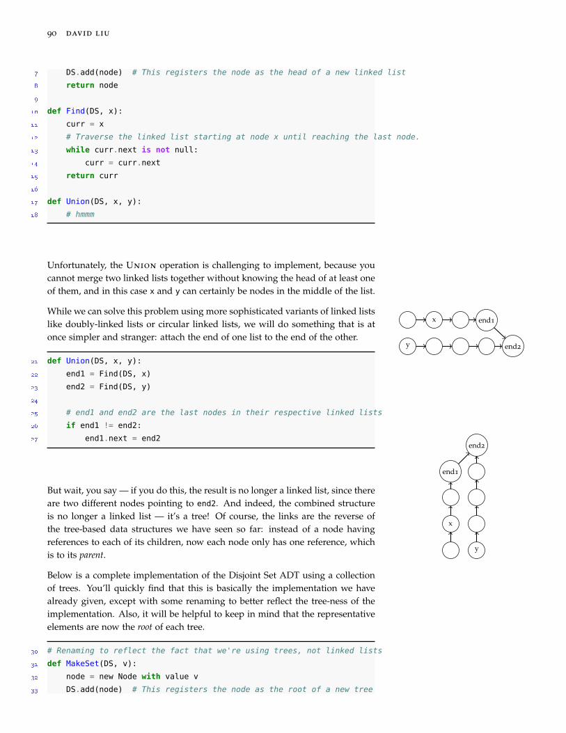
90 david liu

7 DS.add(node) # This registers the node as the head of a new linked list

8 return node

9

10 def Find(DS, x):

11 curr = x

12 # Traverse the linked list starting at node x until reaching the last node.

13 while curr.next is not null:

14 curr = curr.next

15 return curr

16

17 def Union(DS, x, y):

18 # hmmm

Unfortunately, the Union operation is challenging to implement, because youcannot merge two linked lists together without knowing the head of at least oneof them, and in this case x and y can certainly be nodes in the middle of the list.

While we can solve this problem using more sophisticated variants of linked listslike doubly-linked lists or circular linked lists, we will do something that is atonce simpler and stranger: attach the end of one list to the end of the other.

x end1

y end2


22 end1 = Find(DS, x)

23 end2 = Find(DS, y)

24

25 # end1 and end2 are the last nodes in their respective linked lists

26 if end1 != end2:

27 end1.next = end2

But wait, you say — if you do this, the result is no longer a linked list, since thereare two different nodes pointing to end2. And indeed, the combined structureis no longer a linked list — it’s a tree! Of course, the links are the reverse ofthe tree-based data structures we have seen so far: instead of a node havingreferences to each of its children, now each node only has one reference, whichis to its parent.

x

end1

y

end2

Below is a complete implementation of the Disjoint Set ADT using a collectionof trees. You’ll quickly find that this is basically the implementation we havealready given, except with some renaming to better reflect the tree-ness of theimplementation. Also, it will be helpful to keep in mind that the representativeelements are now the root of each tree.

30 # Renaming to reflect the fact that we're using trees, not linked lists



33 DS.add(node) # This registers the node as the root of a new tree


34 return node

35

36 def Find(DS, x):

37 curr = x

38 while curr.parent is not null:

39 curr = curr.parent

40 return curr

41


43 root1 = Find(DS, x)

44 root2 = Find(DS, y)

45

46 # root1 and root2 are the roots of their respective trees

47 if root2 != root2

48 root1.parent = root2

Runtime analysis

Now, let us briefly analyse the running time of the operations for this tree-baseddisjoint set implementation. The MakeSet operation clearly takes Θ(1) time,while both Find and Union take time proportional to the distance from theinputs to the root of their respective trees. In the worst case, this is Θ(h), where

Remember that the disjoint set collec-tion can contain multiple trees, eachwith their own height. The runningtime of Find and Union depends onthe trees that are involved.

h is the maximum height of any tree in the collection.

Of course, as with general trees, it is possible for the heights to be proportionalto n, the total number of items stored in all of the sets, leading to a worst-caserunning time of Θ(n).

Heuristics for tree-based disjoint sets

It is quite discouraging that our initial tree-based implementation of disjoint setshas worst-case running time that is linear in the total number of items stored.After all, we could come up with a linear time implementation of disjoint setsthat simply stores pairs (item, set representative) in a list, and loop over thelist for Find and Union.

However, just as we improved our BST implementation of dictionaries by im-posing more structure on the tree itself, we will now investigate two heuristicsused to reduce the height of the trees for our disjoint set implementation.

Union-by-rank

One idea we borrow from AVL trees is the idea of enforcing some local propertyof nodes to try to make the whole tree roughly balanced. While we do not have

92 david liu

to enforce the binary search tree property here, we are limited in two other ways:

• We do not want to have to traverse a full tree every time we perform a Union.

• Nodes only have references to their parent, but not their children (child ref-erences turn out to be unnecessary).

Rather than have nodes keep track of their height or balance factor, we will storean attribute called rank, which has the following definition:

Definition 8.1 (rank (disjoint sets)). The rank of a node in a disjoint set tree isdefined recursively as follows:

• The rank of a leaf is 0.

• The rank of an internal node is one plus the maximum rank of its children.

It is no coincidence that this definition is closely related to the recursive defi-nition of tree height you may have seen before. You may wonder, then, whywe don’t just use height. Indeed, we could for this section; but for the secondheuristic we’ll study, we want an attribute that never decreases, even when atree’s height decreases. And so for consistency, we use the same attribute forboth heuristics.

With this notion of rank in hand, we no longer arbitrarily choose the mergedtree root in a Union; instead, we always use the root with the larger rank.The intuition is that if we merge a bigger tree and a smaller tree, we can makethe smaller tree a subtree of the bigger tree without changing the bigger tree’sheight. We call this modification of the basic Union algorithm the union-by-rank heuristic.

14 # Union-by-rank



17 DS.add(node) # This registers the node as the root of a new tree

18 node.rank = 0 # set the rank

19 return node

20


22 root1 = Find(DS, x)

23 root2 = Find(DS, y)

24

25 if root1 == root2:

26 return

27

28 # root1 and root2 are the roots of their respective trees

29 # Choose the one with the larger rank as the new root.

30 # Only need to increment a rank when the two root ranks are equal.

31 if root1.rank > root2.rank:



33 else if root1.rank < root2.rank:


35 else:


37 root2.rank = root2.rank + 1

Observe that the rank of a node onlyever increases by 1, and only if it ismerged with a node of the same rank.In all other cases, Union does notincrease rank.

Let us make our previous intuition about attaching the “smaller” tree to the“bigger” one more precise in the following two lemmas.

Lemma 8.1 (Rank for disjoint sets). Let T be a tree generated by a series ofMakeSet and Union operations using the union-by-rank heuristic. Let r bethe rank of the root of T, and n be the number of nodes in T. Then 2r ≤ n.

Proof. We will prove that the property 2r ≤ n is an invariant that is preserved byevery MakeSet and Union operation.

For MakeSet, the new tree that is created has one node, and its root has rank0. The theorem holds in this case, since 20 = 1 ≤ 1.

For Union, suppose we take the union of two trees T1 and T2, with sizes n1 andn2 and ranks r1 and r2, respectively. We assume that 2r1 ≤ n1 and 2r2 ≤ n2. Letn = n1 + n2 be the number of nodes in the union tree, and r be the rank of theroot of the union tree. We want to prove that 2r ≤ n.

Case 1: r1 > r2. In this case, r = r1, since the root of T1 is chosen as the root ofthe union tree, and its rank doesn’t change. So then 2r = 2r1 ≤ n1 < n, so theproperty still holds. The same argument works for the case that r2 < r1 as well,by switching the 1’s and 2’s.

Case 2: r1 = r2. In this case, the root of T1 is selected to be the new root, and itsrank is increased by one: r = r1 + 1. Then since 2r1 ≤ n1 and 2r2 ≤ n2, we get2r1 + 2r2 ≤ n1 + n2 = n. Since r1 = r2, 2r1 + 2r2 = 2r1+1 = 2r, and the propertyholds.

We’ll leave it as an exercise to prove the second lemma, which says that the rankreally is a good approximation of the height of the tree.

Lemma 8.2. Let T be a tree generated by a series of MakeSet and Union

operations using the union-by-rank heuristic, and let r be the rank of its root.Then the height of T is equal to r + 1.

With these two lemmas, we can prove the following much-improved bound onthe worst-case running time of our disjoint set operations when we use theunion-by-rank heuristic.

Theorem 8.3 (Worst-case running time using union-by-rank). The worst-caserunning time of Find and Union for the disjoint set implementation usingunion-by-rank is Θ(log n), where n is the number of items stored in the sets.

94 david liu

Proof. Note that the manipulations involving the new rank attribute in the im-plementation are all constant time, and so don’t affect the asymptotic runningtime of these algorithms. So, by our previous argument, the worst-case runningtime of these two operations is still Θ(h), where h is the maximum height of atree in the disjoint set data structure. Now we show that h = O(log n), where nis the total number of items stored in the sets.

Let T be a tree in the data structure with height h, r be the rank of the root ofthis tree, and n′ be the size of this tree. By our previous two lemmas, we have

Obviously, n′ ≤ n.the chain of inequalities

h = r + 1 ≤ log n′ + 1 ≤ log n + 1.

It follows immediately that h = O(log n). We leave the lower bound as anexercise.


Exercise Break!

8.1 Prove that the worst-case running time of a Find or Union operation whenusing union-by-rank is Ω(log n), where n is the number of items stored in thesets.

8.2 Suppose we have a disjoint set collection consisting of n items, with each itemin its own disjoint set.

Then, suppose we perform k Union operations using the union-by-rankheuristic, where k < n, followed by one Find operation. Give a tight asymp-totic bound on the worst-case running time of this Find operation, in termsof k (and possibly n).

Path compression

Our previous heuristic involved some optimization on the Union operationto get a better bound on the height of the trees in the disjoint set collection.Such mutating operations are a natural place for optimization: given that weare modifying the structure of the sets, it is natural to think about how to bestdo this. In this section, we will investigate a different heuristic, which performsa mutation operation in a previously read-only operation, Find. This drawsinspiration from the common query optimization of caching, in which the resultof a query are saved to make future repetitions of the same query faster. When

Think of “query” here as a generic termfor any computation that returns avalue, like Find.

we perform a Find operation on a node x, we will explicitly store the resultingset representative by restructuring the tree so that performing a Find on thatsame node in the future is guaranteed to run in constant time.

When a Find operation takes a long time, it is because the input node is quite farfrom the root of the tree, and all of the node’s ancestors must be traversed. Thekey insight is that unlike most other tree operations we have looked at in thiscourse, there is no reason to preserve the structure of the tree during a Find operation.Because each node in a tree only cares about its set representative, there is noreason a node shouldn’t just point directly to it, other than the fact that setrepresentatives change during Unions. So the path compression heuristic isthe following: after the set representative is found, all of the nodes traversed

Hopefully it is clear why this is called“path compression.” The (potentiallylong) path traversed from input node toroot is split up, with each node on thepath now “compressed” by becoming achild of the root.

have their parent attribute set to this set representative. In purely tree terms,the tree is restructured so that the node and all of its ancestors are made directchildren of the root.

96 david liu

40 # Path compression

41 def Find(DS, x):

42 root = x

43 # After this loop, root is the root of the tree containing x.

44 while root.parent is not null:

45 root = root.parent

46

47 # Path compression: set all ancestors of x to be children of root.

48 curr = x

49 while curr.parent is not null:

50 next_curr = curr.parent

51 curr.parent = root

52 curr = next_curr

Running time analysis for path compression

Despite all this fanfare about path compression, it is important to realize thatthis heuristic does not improve the speed of a Find operation that has a longpath — this operation still takes time proportional to the length of the path, andthe worst-case running time is still Θ(n), where n is the number of items inthe sets. This is true of caching in general: the first time a query is run, there

Keep in mind that we don’t have theunion-by-rank guarantee here, sothe maximum height of a tree is thenumber of items in the disjoint sets.

is no speedup due to previous computations, because there are no previouscomputations!

What path compression does guarantee is that any subsequent Find operationson any nodes along the compressed path will take constant time. Wheneveryou hear a phrase like “operation makes future operations faster,” you shouldthink about amortized analysis: even if the initial operation is slow, perhaps itsrunning time cost can be amortized across multiple (faster) Find operations.And it turns out that with the path compression heuristic, the amortized runningtime of Find operations has a substantial improvement over the worst-case Θ(n)bound. We will only perform a special case of the full analysis here. You’ll findthat this is sufficient to get the general idea, while being able to ignore someextra parameters that come with the most generalized version.

One reminder before we go into the proof. This proof uses the notion of noderank from the previous section, with one important clarification: node rank isonly updated during a merge operation, and only if the node is the new rootof the union tree. This is quite important because path compression can causetree height to decrease, so keep in mind that rank is not the same as height, anddoes not change for any node during Find. There are four important propertiesof node rank to keep in mind (we leave proofs as exercises):

• The rank of a node is always between 0 and n− 1.

• Ranks are strictly increasing as you go up a tree; the rank of a node is always


less than the rank of its parent.

• The rank of a node only ever increases, and only during a Union operation.

• Let x be a node. The rank of the parent of x only ever increases — not onlywhen a Union operation causes the parent node of x to increase in rank, butalso when a Find operation causes x to get a different parent node.

Theorem 8.4 (Amortized analysis of path compression (special case)). Supposewe use a disjoint set implementation that uses the path compression heuristic.Let n be a power of two, and consider a sequence of n MakeSet operations,followed by any number of Union operations mixed with n Find operations.

Then the total cost of all n Find operations is O(n log n). Or in other words, theamortized cost of an individual Find operation is O(log n).

Proof. We will use the aggregate method to perform the amortized analysis here,but in a more advanced way: rather than computing the cost of each Find

operation separately and adding them up, we will attempt to add up all thecosts at once, without knowing the value of any individual cost.

The key insight is that for any individual Find operation, its running time isproportional to the number of edges traversed from the input node up to theroot. In this proof, we will call the path traversed by a Find operation a findpath. So we define the collection of edges F in the n find paths, allowing forduplicates in F because the same edge can belong to multiple find paths. Toanalyse this, we consider the collection of edges F that are traversed by any oneof the n Find operations. Then the total cost of the sequence of n Find operationsis simply |F |, and the amortized cost of an individual Find operation is |F |/n.

The second key idea is to partition F based on the differential rank of the end-points of each edge. For each 1 ≤ i ≤ log n, define the set

Fi = (x, y) ∈ F | 2i−1 ≤ rank(y)− rank(x) < 2i.

Note that the final set, Flog n, contains an upper bound on the rank differenceThe notation (x, y) indicates an edgetraversed from node x to its parent y.So rank(y) ≥ rank(x).

of 2log n = n, so each edge belongs to exactly one of these sets. So |F | = ∑ |Fi|,and our task is now to bound the sizes of each Fi. What can we say about thesize of an Fi? It turns out that we can say quite a bit, if we do some carefulcounting.

First, we divide each Fi into two subgroups based on the relative positions ofthe edges in their find paths. We say that an edge e ∈ Fi is a last edge if it is theedge in Fi closest to the set representative of its tree. Otherwise, we say that theedge e is a middle edge. We let Li and Mi be the set of last and middle edgesfrom Fi, respectively.

This is a little abstract, so let’s make it more concrete. Suppose we have a findpath that contains three edges e1, e2, e3 from Fi (plus possibly many other edges).Suppose e3 is closest to the root of the tree. Then e3 is a last edge, and e1 and e2

are middle edges. In general, if multiple edges from Fi appear on the same findpath, exactly one of them will be a last edge, and all the others will be middleedges.

98 david liu

Since each edge in Fi is either a last or middle edge, |Fi| = |Li|+ |Mi|. RatherDon’t worry, we aren’t going to subdi-vide any further! Geez.than computing the size of Fi, we want to compute the sizes of Li and Mi.

Since there are a total of n Find operations in the sequence, there are n findpaths. Each find path can have at most one last edge for each rank difference, so|Li| ≤ n.

Now let us count the size of |Mi|. We’ll do this by looking at individual nodes.Consider a middle edge e ∈ Mi, which goes from node x to its parent y. At thetime of the Find operation that this edge is traversed, we know the followingthings:

x

y

z

e

e′

• There is another edge e′ ∈ Fi that is closer than e to the root of the tree (sincee is a middle edge).

• y is not the set representative of the tree (since it can’t be the root).

Let z be the set representative for this tree; so s is distinct from x and y. Sincethe nodes visited on the path from y to z have increasing rank, and e′ separatesy and z along this path, we know that rank(z)− rank(y) ≥ 2i−1.

Checkpoint: this inequality only usesthe fact that the edge e′ ∈ Fi is betweenw and s. We haven’t yet used the factthat e is also in Fi .

Furthermore, due to path compression, after this Find operation is complete, zbecomes the new parent of x. Here is the third big idea. The actual node changeitself doesn’t matter to our proof; what does matter is that from the point ofview of x, its parent’s rank has increased by at least 2i−1.

Remember, no node actually changedits rank. It’s just that the parent of xchanged to one with a bigger rank.Why is this such a big deal? We can use this to prove the following claim.

Proposition 8.5. Let x be a node. There are at most two edges in Mi that startat x.

Proof. Suppose for a contradiction that there are three edges (x, y1), (x, y2),(x, y3) ∈ Mi. Also, assume that by the time a Find operation visits the edge(x, y3), previous Find operations have already visited (x, y1) and (x, y2). Theprevious observation tells us that the rank of the parent of x must have increasedby at least 2 · 2i−1 = 2i, i.e., rank(y3) ≥ rank(y1) + 2i.

This is finally where we use the fact that these edges are inMi! This tells us thatrank(y1) ≥ rank(x) + 2i−1, and so we get rank(y3) ≥ rank(x) + 2i + 2i−1. But thefact that (x, y3) ∈ Mi means that rank(y3) ≤ rank(x) + 2i, a contradiction.

Since the above claim is true for any node x, this means that each of the n nodesin the disjoint sets can be the starting point for at most two edges in Mi. Thisimplies that |Mi| ≤ 2n.

It is actually quite remarkable that thesize of each |Mi | doesn’t depend on iitself.Putting this all together yields a bound on the size of F :


|F | =log n

∑i=1|Fi|

=log n

∑i=1|Li|+ |Mi|

≤log n

∑i=1

n + 2n

= 3n log n

In other words, the total number of edges visited by the n Find operations isO(n log n), and this is the aggregate cost of the n Find operations.

Combining the heuristics: a tale of incremental analyses

We have seen that both union-by-rank and path compression can each be usedto improve the efficiency of the Find operation. We have performed the anal-ysis on them separately, but what happens when we apply both heuristics atonce? This is not merely an academic matter: we have seen that it is extremelystraightforward to implement each one, and because union-by-rank involves achange to Union and path compression involves a change to Find, it is veryeasy to combine them in a single implementation.

The challenge here is performing the running time analysis on the combinedheuristics. We can make some simple observations:

• The worst-case bound of Θ(log n) for Find from union-by-rank still applies,since it is possible to do a bunch of Unions, and then a single Find on a leafwhen the tree has height Θ(log n).

• The amortized analysis we did for path compression still holds, since all thekey properties of rank that we used still hold.

In other words, the two analyses that we performed for the two heuristics stillapply when we combine them. The only lingering question is the amortized costof a Find operation, for which we only proved an upper bound in the previoussection. Given that our analysis for path compression alone had to accommodatefor a node of rank n, while union-by-rank ensured that a node’s rank is at mostlog n, there may be hope for a better amortized cost.

And indeed, there is. What follows is a tour of the major results in the historyof this disjoint set implementation, going from its humble beginnings to theprecise analysis we take for granted today. It is truly a remarkable story of analgorithm whose ease of implementation belied the full subtlety of its runningtime analysis.

The first known appearance of this disjoint set implementation, which combinedboth union-by-rank and path compression, was in a paper by Bernard A. Galler

100 david liu

and Michael J. Fischer in 1964. However, the authors of this paper did notperform a precise analysis of their algorithm, and in fact the question of howefficient this was, really, took almost two decades to resolve.

In 1972, Fischer proved that the amortized cost of each Find operation isO(log log n),already a drastic improvement over the O(log n) bound we proved in the previ-ous section. The next year, John Hopcroft and Jeffrey Ullman published a further

You should be able to modify our proofto get an amortized cost of O(log log n)for the rank bound that union-by-rankgives us.

improvement, showing the amortized cost of Find to be O(log∗ n), where log∗ nis the iterated logarithm function, defined recursively as follows:

log∗ n =

0, if n ≤ 1

1 + log∗(log n), otherwise

In English, this function outputs the number of times the logarithm must beapplied to a number to get a result ≤ 1. To give some context about how slow-growing this function is, we show in a table the largest value of n to get the firstfew natural numbers as output.

If m is the largest number such thatlog∗ m = k, then n = 2m is the largestnumber such that log∗ n = k + 1.

Largest n log∗ n1 0

2 1

4 2

16 3

65536 4

2655365

For context, the estimated number ofatoms in the universe is roughly 2272.While this running time is so close to constant that it seems like this should have

been the end of it, investigation of this function did not stop at the Hopcroft-Ullman result. In 1975, just two years later, Robert Endre Tarjan published hispaper “Efficiency of a Good But Not Linear Set Union Algorithm.” His mainresult was that the amortized cost of each Find operation is Θ(α(n)), whereα(n) is the inverse Ackermann function, a function that grows even more slowlythan the iterated logarithm.

For comparison to the iterated loga-

rithm, α(22265536) = 4.And even more impressive than getting a better upper bound was that Tarjan

was able to show a matching lower bound, i.e., give a sequence of operations sothat the amortized cost of the Find operations when using both union-by-rankand path compression is Ω(α(n)). This showed that no one else would be ableto come along and give a better upper bound for the amortized cost of theseoperations, and the question was settled — almost. At the end of the paper,Tarjan wrote the following (emphasis added):

This is probably the first and maybe the only existing example of a simple algorithmwith a very complicated running time. The lower bound given in Theorem 16 isgeneral enough to apply to many variations of the algorithm, although it is an openproblem whether there is a linear-time algorithm for the online set union problem.On the basis of Theorem 16, I conjecture that there is no linear-time method, andthat the algorithm considered here is optimal to within a constant factor.


In other words, having completed his analysis of the disjoint set data structureusing both union-by-rank and path compression, Tarjan proposed that no otherheuristics would improve the asymptotic amortized cost of Find, nor would anyother completely different algorithm.

And in 1989 (!), Michael Fredman and Michael Saks proved that this was true:any implementation of disjoint sets would have an amortized cost for Find ofΩ(α(n)). This is quite a remarkable statement to prove, as it establishes somekind of universal truth over all possible implementations of disjoint sets — evenones that haven’t been invented yet! Rather than analyse a single algorithm orsingle data structure, they defined a notion of innate hardness for the disjoint setADT itself that would constrain any possible implementation. This idea, thatone can talk about all possible implementations of an abstract data type, or allpossible algorithms solving a problem, is truly one of the most fundamental —and most challenging — pillars of theoretical computer science.

Exercise Break!

8.3 The idea of using an attribute to store the rank of each node is a powerfulone, and can be extended to storing all sorts of metadata about each set.

Use an augmented version of the tree-based disjoint set data structure to sup-port the following two operations, using only linear additional space:

• Max(DS, x): Return the maximum value in the set containing x

• Min(DS, y): Return the minimum value in the set containing y

What is the running time of these two operations?

8.4 Why is it harder to augment this data structure to store the median value ofeach set? More generally, can you characterize the kinds of queries that are“easy” to support using an augmented disjoint set data structure?

8.5 We have seen in Chapter 6 how to use depth-first search (or breadth-firstsearch) to detect cycles in a graph.

Consider the following dynamic version of this problem: we are given n ver-tices, and originally have no edges between them. Then edges are added, oneat a time. Each time an edge is added, we want to report if that edge forms acycle in the graph.

(a) Suppose that each time an edge is added, we perform a depth-first searchstarting at one of its endpoints. What is the amortized cost per edge addi-tion in this case?

(b) Give an algorithm to support this cycle detection using disjoint sets, andanalyse the amortized cost per edge addition in this case.

Data Structures and Analysisdavid/course-notes/csc263.pdf · Lecture Notes for CSC263 (Version 0.2)...

Documents

Transcript of Data Structures and Analysisdavid/course-notes/csc263.pdf · Lecture Notes for CSC263 (Version 0.2)...