Data Structures and Algorithms - Vilniaus …algis/dsax/Data-structures-5.pdfData Structures and...

Data Structures and

Algorithms Course slides: Radix Search, Radix sort,

Bucket sort, Patricia tree

Lecture 10: Searching

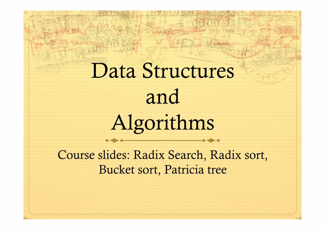
Radix Searching

ò  For many applications, keys can be thought of as numbers

ò  Searching methods that take advantage of digital properties of these keys are called radix searches

ò  Radix searches treat keys as numbers in base M (the radix) and work with individual digits


Radix Searching

ò  Provide reasonable worst-case performance without complication of balanced trees.

ò  Provide way to handle variable length keys.

ò  Biased data can lead to degenerate data structures with bad performance.


The Simplest Radix Search

ò  Digital Search Trees — like BSTs but branch according to the key’s bits.

ò  Key comparison replaced by function that accesses the key’s next bit.


Digital Search Example

A

R H C

S E

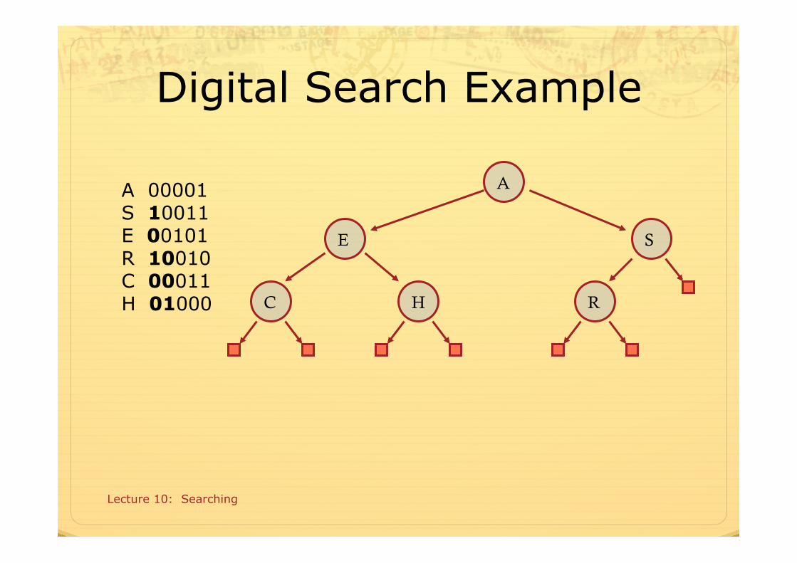
A 00001 S 10011 E 00101 R 10010 C 00011 H 01000

6

Digital Search Trees

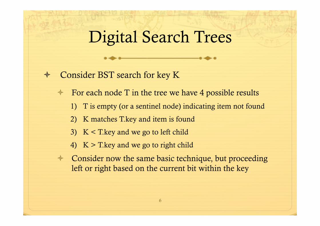
ò  Consider BST search for key K

ò  For each node T in the tree we have 4 possible results

1)  T is empty (or a sentinel node) indicating item not found

2)  K matches T.key and item is found

3)  K < T.key and we go to left child

4)  K > T.key and we go to right child

ò  Consider now the same basic technique, but proceeding left or right based on the current bit within the key

7


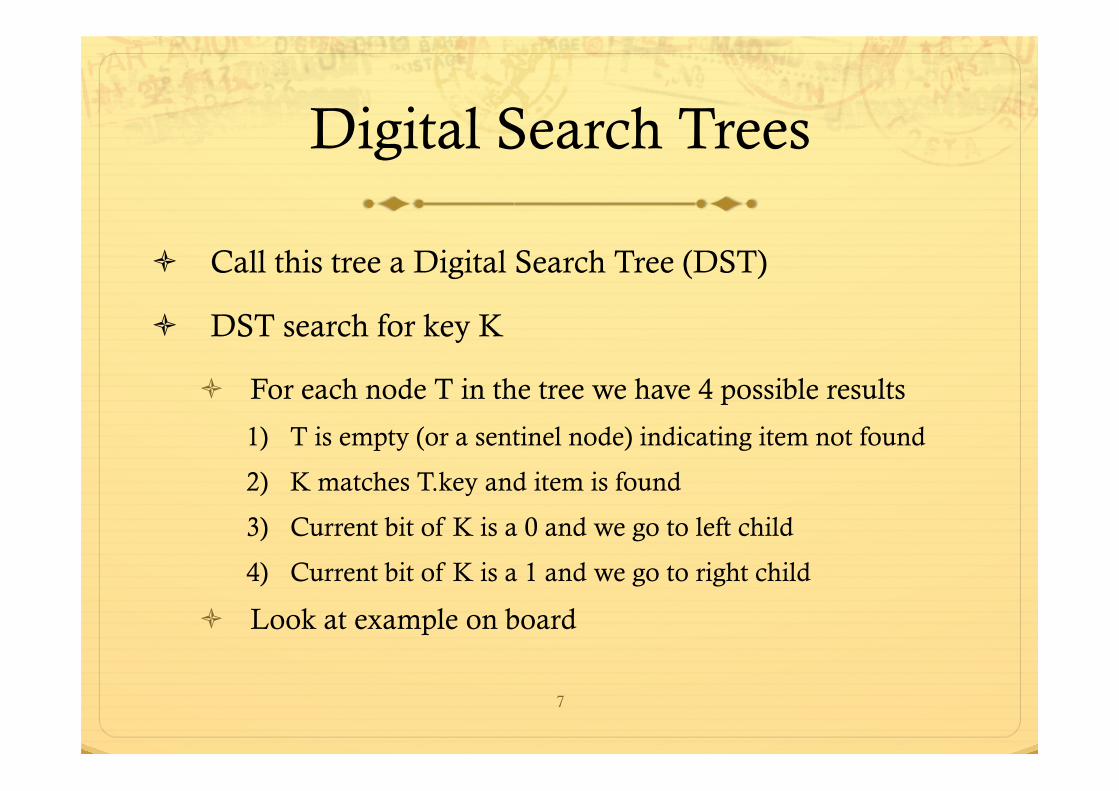
ò  Call this tree a Digital Search Tree (DST)

ò  DST search for key K

ò  For each node T in the tree we have 4 possible results

1)  T is empty (or a sentinel node) indicating item not found

2)  K matches T.key and item is found

3)  Current bit of K is a 0 and we go to left child

4)  Current bit of K is a 1 and we go to right child

ò  Look at example on board

8


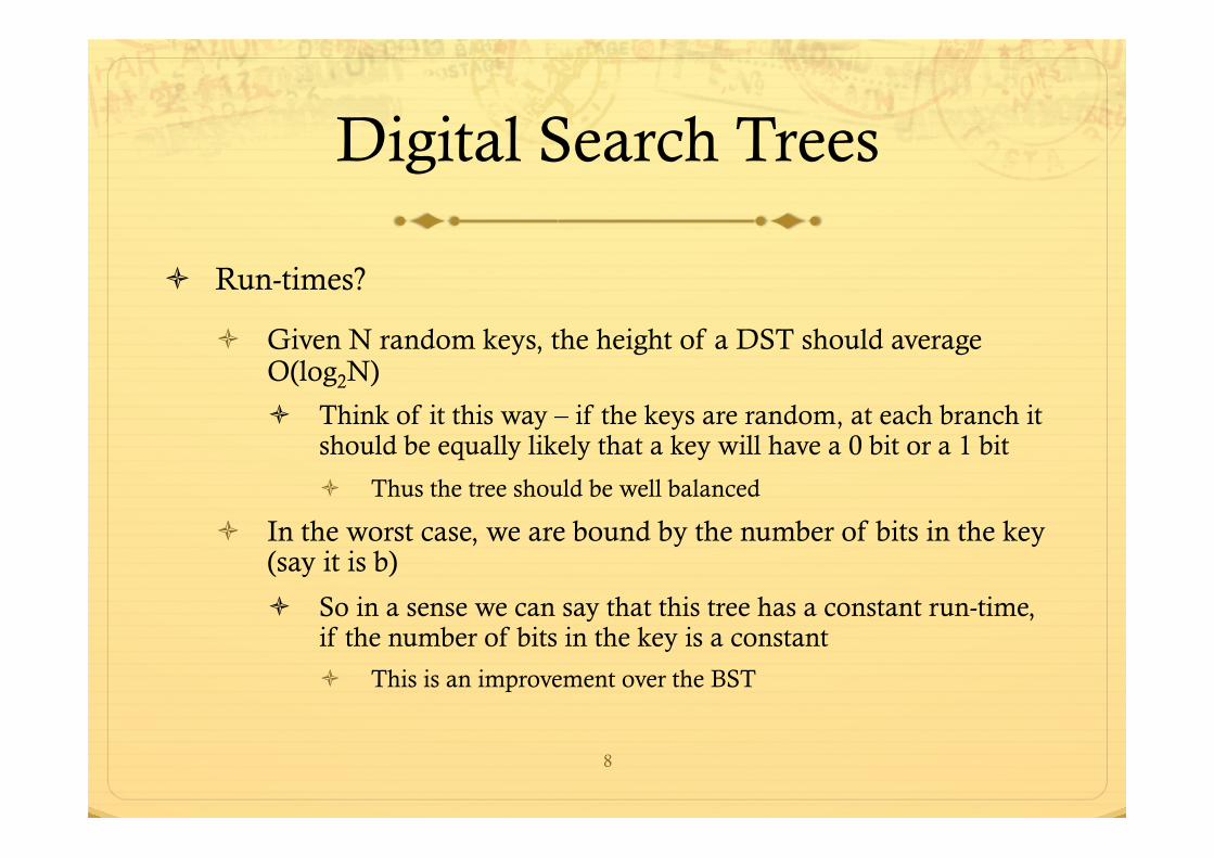
ò  Run-times?

ò  Given N random keys, the height of a DST should average O(log2N)

ò  Think of it this way – if the keys are random, at each branch it should be equally likely that a key will have a 0 bit or a 1 bit

ò  Thus the tree should be well balanced

ò  In the worst case, we are bound by the number of bits in the key (say it is b)

ò  So in a sense we can say that this tree has a constant run-time, if the number of bits in the key is a constant

ò  This is an improvement over the BST

9


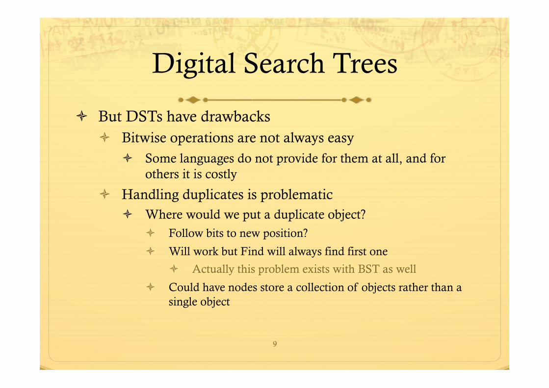
ò  But DSTs have drawbacks ò  Bitwise operations are not always easy

ò  Some languages do not provide for them at all, and for others it is costly

ò  Handling duplicates is problematic ò  Where would we put a duplicate object?

ò  Follow bits to new position?

ò  Will work but Find will always find first one

ò  Actually this problem exists with BST as well

ò  Could have nodes store a collection of objects rather than a single object

10


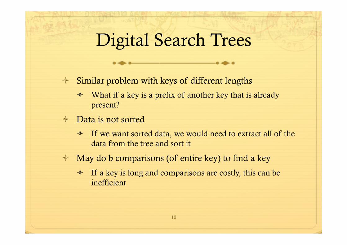
ò  Similar problem with keys of different lengths

ò  What if a key is a prefix of another key that is already present?

ò  Data is not sorted

ò  If we want sorted data, we would need to extract all of the data from the tree and sort it

ò  May do b comparisons (of entire key) to find a key

ò  If a key is long and comparisons are costly, this can be inefficient


Digital Search

ò  Requires O(log N) comparisons on average

ò  Requires b comparisons in the worst case for a tree built with N random b-bit keys


Digital Search

ò  Problem: At each node we make a full key comparison — this may be expensive, e.g. very long keys

ò  Solution: store keys only at the leaves, use radix expansion to do intermediate key comparisons


Radix Tries

ò  Used for Retrieval [sic]

ò  Internal nodes used for branching, external nodes used for final key comparison, and to store data


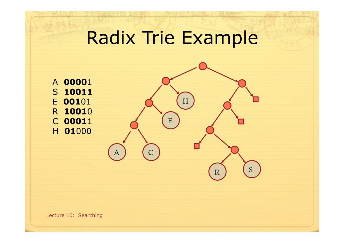
Radix Trie Example

S

A 00001 S 10011 E 00101 R 10010 C 00011 H 01000

R

E

C A

H


Radix Tries

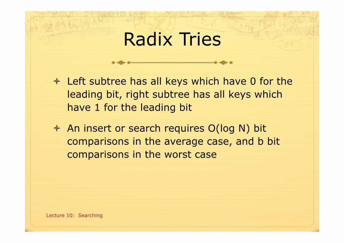
ò  Left subtree has all keys which have 0 for the leading bit, right subtree has all keys which have 1 for the leading bit

ò  An insert or search requires O(log N) bit comparisons in the average case, and b bit comparisons in the worst case


Radix Tries

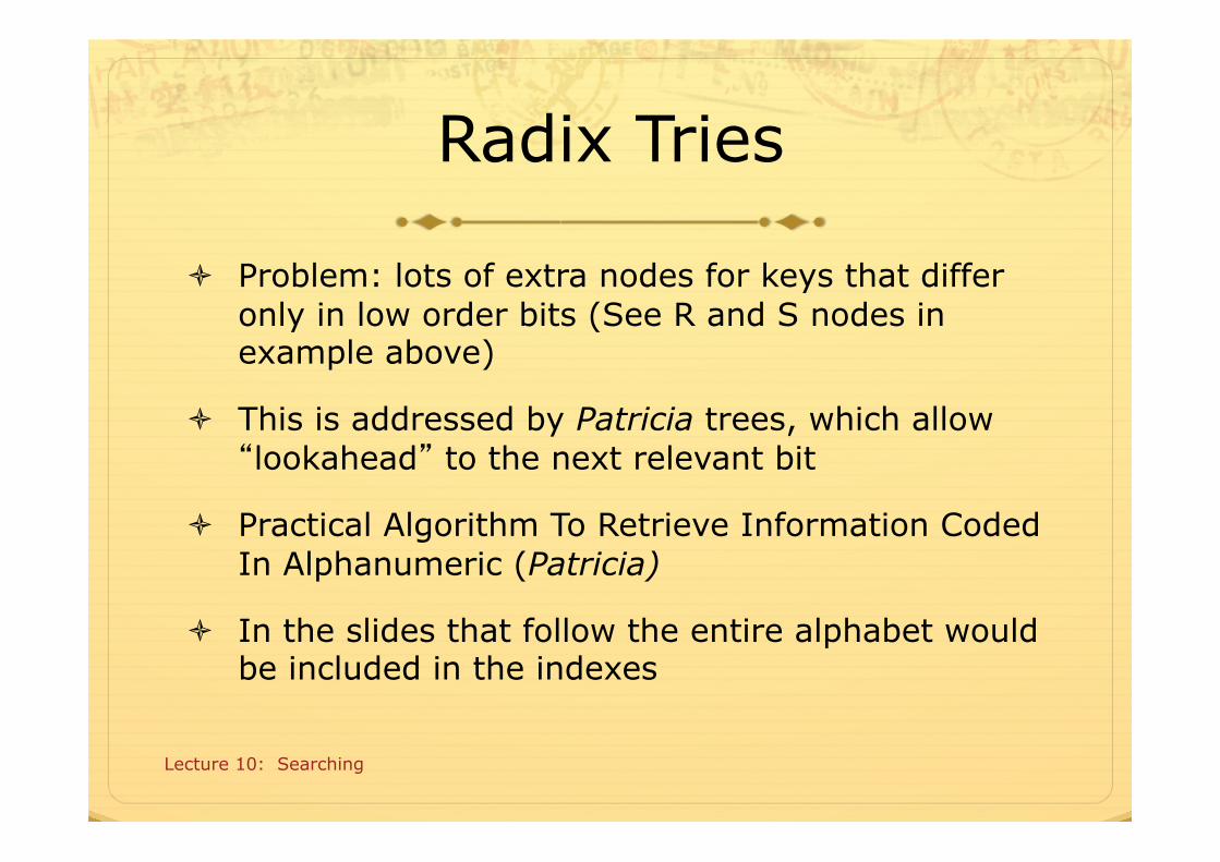
ò  Problem: lots of extra nodes for keys that differ only in low order bits (See R and S nodes in example above)

ò  This is addressed by Patricia trees, which allow “lookahead” to the next relevant bit

ò  Practical Algorithm To Retrieve Information Coded In Alphanumeric (Patricia)

ò  In the slides that follow the entire alphabet would be included in the indexes

17

Radix Search Tries

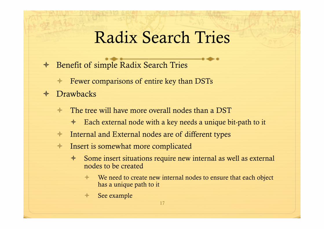
ò  Benefit of simple Radix Search Tries

ò  Fewer comparisons of entire key than DSTs

ò  Drawbacks

ò  The tree will have more overall nodes than a DST

ò  Each external node with a key needs a unique bit-path to it

ò  Internal and External nodes are of different types

ò  Insert is somewhat more complicated

ò  Some insert situations require new internal as well as external nodes to be created

ò  We need to create new internal nodes to ensure that each object has a unique path to it

ò  See example

18

Radix Search Tries

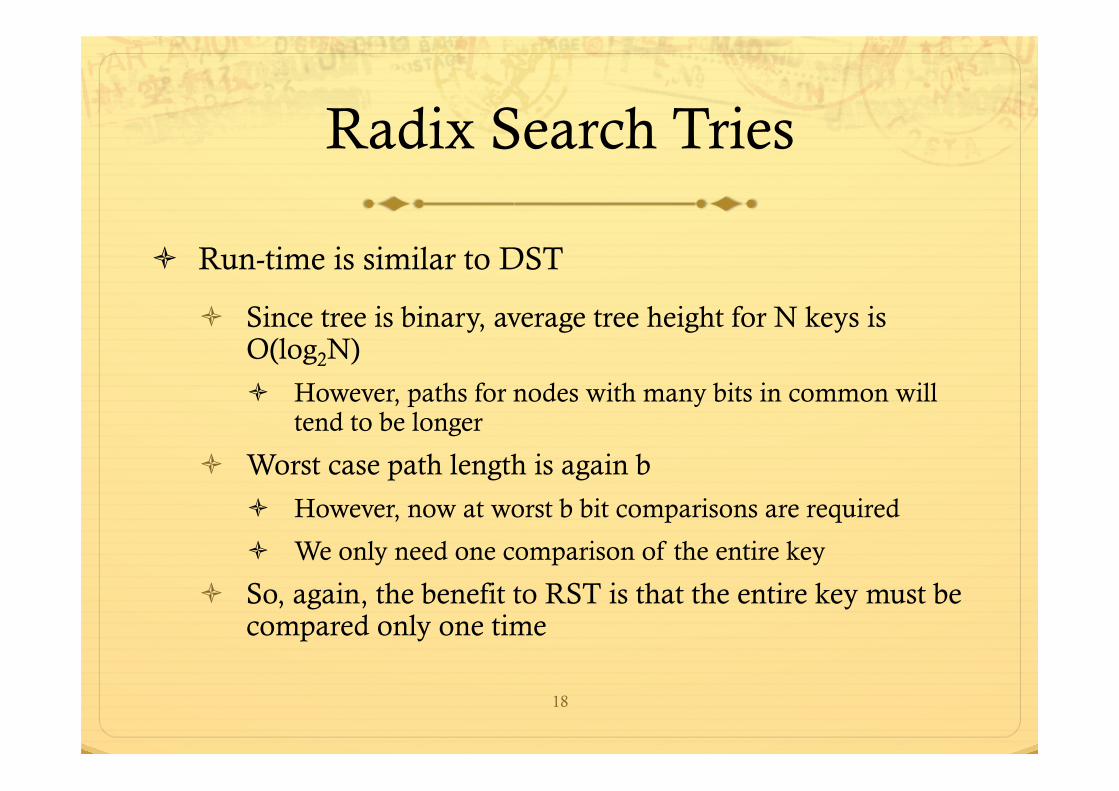
ò  Run-time is similar to DST

ò  Since tree is binary, average tree height for N keys is O(log2N)

ò  However, paths for nodes with many bits in common will tend to be longer

ò  Worst case path length is again b

ò  However, now at worst b bit comparisons are required

ò  We only need one comparison of the entire key

ò  So, again, the benefit to RST is that the entire key must be compared only one time

19

Improving Tries

ò  How can we improve tries?

ò  Can we reduce the heights somehow?

ò  Average height now is O(log2N)

ò  Can we simplify the data structures needed (so different node types are not required)?

ò  Can we simplify the Insert?

ò  We will examine a couple of variations that improve over the basic Trie

Bucket-Sort and Radix-Sort 20

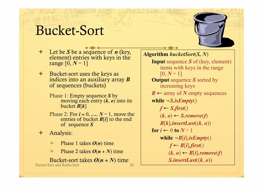
Bucket-Sort ò  Let be S be a sequence of n (key,

element) entries with keys in the range [0, N - 1]

ò  Bucket-sort uses the keys as indices into an auxiliary array B of sequences (buckets)

Phase 1: Empty sequence S by moving each entry (k, o) into its bucket B[k]

Phase 2: For i = 0, …, N - 1, move the entries of bucket B[i] to the end of sequence S

ò  Analysis:

ò  Phase 1 takes O(n) time

ò  Phase 2 takes O(n + N) time

Bucket-sort takes O(n + N) time

Algorithm bucketSort(S, N) Input sequence S of (key, element) items with keys in the range [0, N - 1] Output sequence S sorted by increasing keys B ← array of N empty sequences while ¬S.isEmpty()

f ← S.first() (k, o) ← S.remove(f) B[k].insertLast((k, o))

for i ← 0 to N - 1 while ¬B[i].isEmpty() f ← B[i].first() (k, o) ← B[i].remove(f) S.insertLast((k, o))

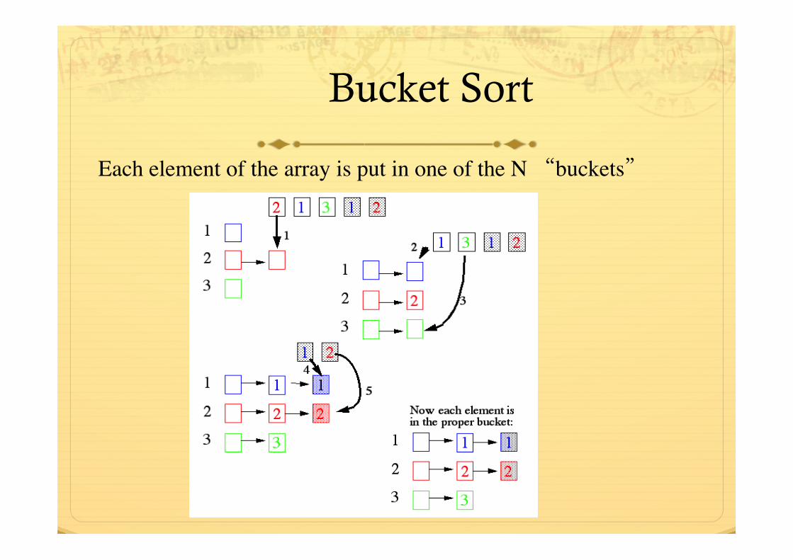
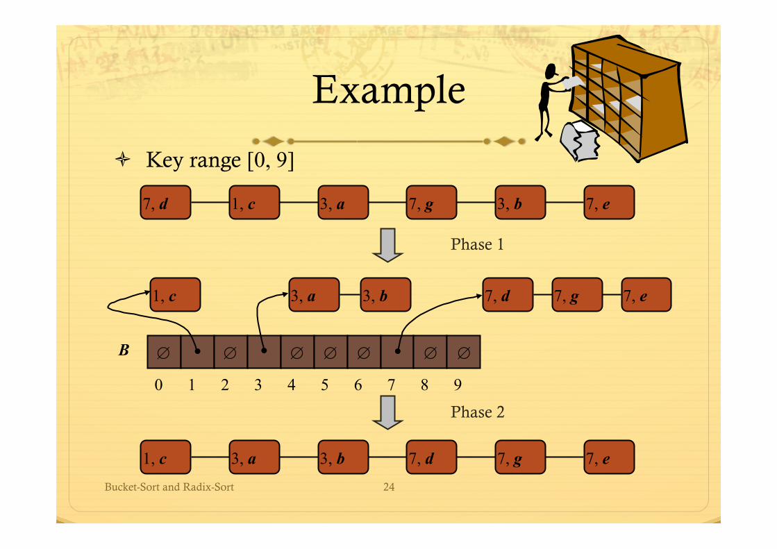
Bucket Sort

Each element of the array is put in one of the N “buckets”

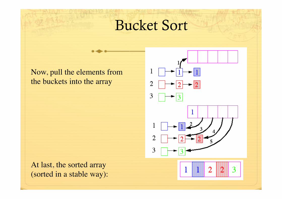
Bucket Sort

Now, pull the elements from the buckets into the array

At last, the sorted array (sorted in a stable way):


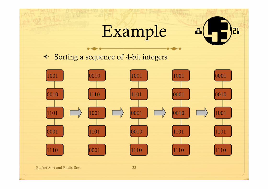
Example ò  Sorting a sequence of 4-bit integers

1001

0010

1101

0001

1110

0010

1110

1001

1101

0001

1001

1101

0001

0010

1110

1001

0001

0010

1101

1110

0001

0010

1001

1101

1110


Example

ò  Key range [0, 9]

7, d 1, c 3, a 7, g 3, b 7, e

1, c 3, a 3, b 7, d 7, g 7, e

Phase 1

Phase 2

0 1 2 3 4 5 6 7 8 9

B

1, c 7, d 7, g 3, b 3, a 7, e

∅ ∅ ∅ ∅ ∅ ∅ ∅


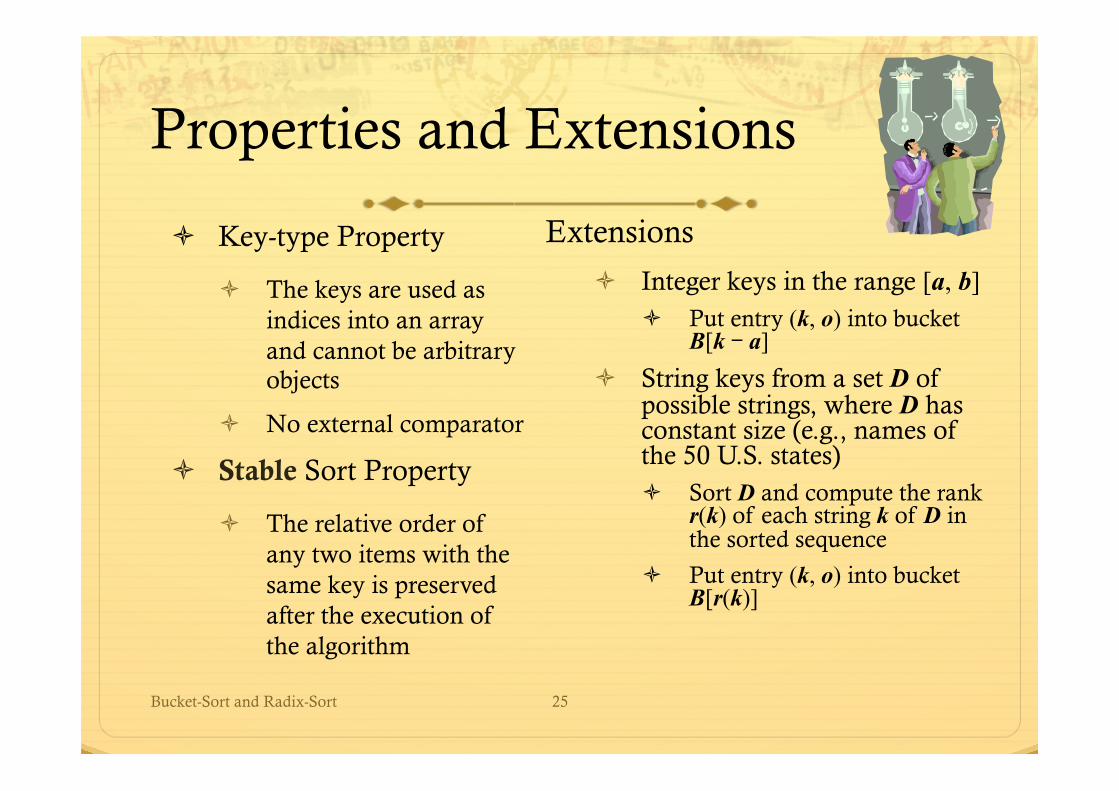
Properties and Extensions

ò  Key-type Property

ò  The keys are used as indices into an array and cannot be arbitrary objects

ò  No external comparator

ò  Stable Sort Property

ò  The relative order of any two items with the same key is preserved after the execution of the algorithm

Extensions

ò  Integer keys in the range [a, b] ò  Put entry (k, o) into bucket

B[k - a] ò  String keys from a set D of

possible strings, where D has constant size (e.g., names of the 50 U.S. states) ò  Sort D and compute the rank

r(k) of each string k of D in the sorted sequence

ò  Put entry (k, o) into bucket B[r(k)]


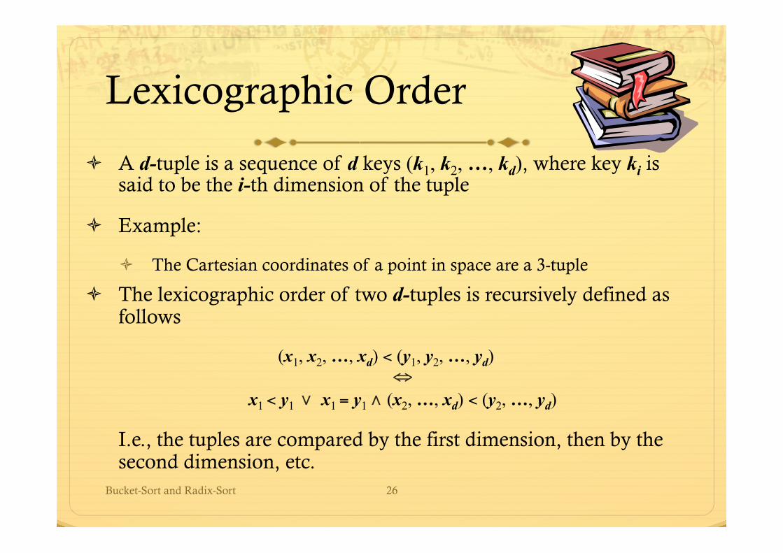
Lexicographic Order

ò  A d-tuple is a sequence of d keys (k1, k2, …, kd), where key ki is said to be the i-th dimension of the tuple

ò  Example:

ò  The Cartesian coordinates of a point in space are a 3-tuple

ò  The lexicographic order of two d-tuples is recursively defined as follows

(x1, x2, …, xd) < (y1, y2, …, yd) ⇔

x1 < y1 ∨ x1 = y1 ∧ (x2, …, xd) < (y2, …, yd)

I.e., the tuples are compared by the first dimension, then by the second dimension, etc.


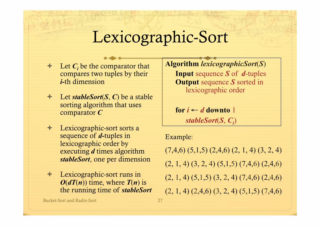
Lexicographic-Sort

ò  Let Ci be the comparator that compares two tuples by their i-th dimension

ò  Let stableSort(S, C) be a stable sorting algorithm that uses comparator C

ò  Lexicographic-sort sorts a sequence of d-tuples in lexicographic order by executing d times algorithm stableSort, one per dimension

ò  Lexicographic-sort runs in O(dT(n)) time, where T(n) is the running time of stableSort

Algorithm lexicographicSort(S) Input sequence S of d-tuples Output sequence S sorted in lexicographic order

for i ← d downto 1

stableSort(S, Ci)

Example:

(7,4,6) (5,1,5) (2,4,6) (2, 1, 4) (3, 2, 4)

(2, 1, 4) (3, 2, 4) (5,1,5) (7,4,6) (2,4,6)

(2, 1, 4) (5,1,5) (3, 2, 4) (7,4,6) (2,4,6)

(2, 1, 4) (2,4,6) (3, 2, 4) (5,1,5) (7,4,6)


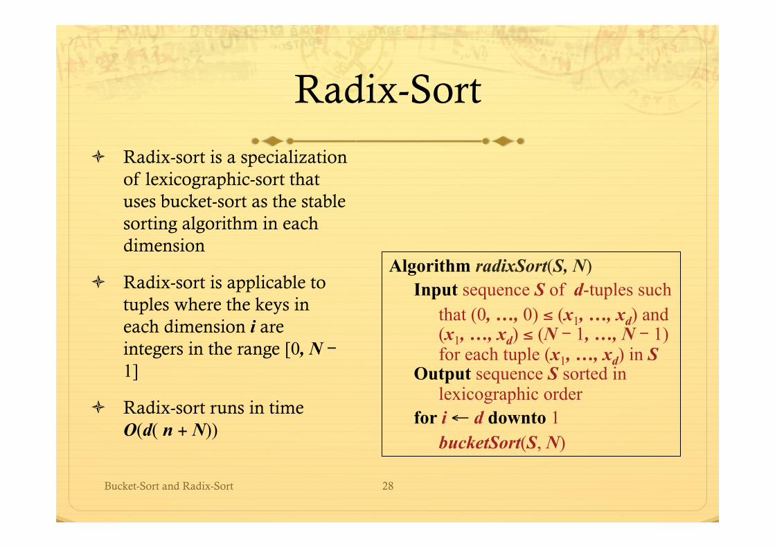
Radix-Sort

ò  Radix-sort is a specialization of lexicographic-sort that uses bucket-sort as the stable sorting algorithm in each dimension

ò  Radix-sort is applicable to tuples where the keys in each dimension i are integers in the range [0, N - 1]

ò  Radix-sort runs in time O(d( n + N))

Algorithm radixSort(S, N) Input sequence S of d-tuples such that (0, …, 0) ≤ (x1, …, xd) and (x1, …, xd) ≤ (N - 1, …, N - 1) for each tuple (x1, …, xd) in S Output sequence S sorted in lexicographic order for i ← d downto 1

bucketSort(S, N)


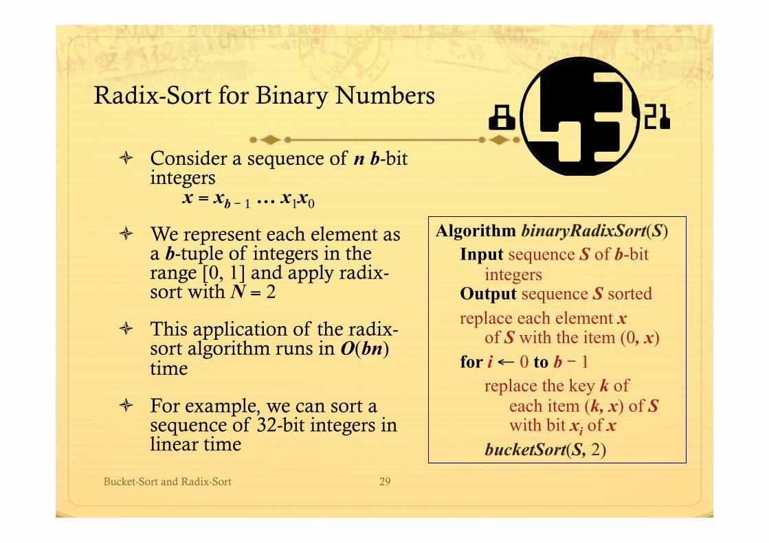
Radix-Sort for Binary Numbers

ò  Consider a sequence of n b-bit integers

x = xb - 1 … x1x0

ò  We represent each element as a b-tuple of integers in the range [0, 1] and apply radix-sort with N = 2

ò  This application of the radix-sort algorithm runs in O(bn) time

ò  For example, we can sort a sequence of 32-bit integers in linear time

Algorithm binaryRadixSort(S) Input sequence S of b-bit integers Output sequence S sorted replace each element x of S with the item (0, x) for i ← 0 to b - 1 replace the key k of each item (k, x) of S with bit xi of x bucketSort(S, 2)

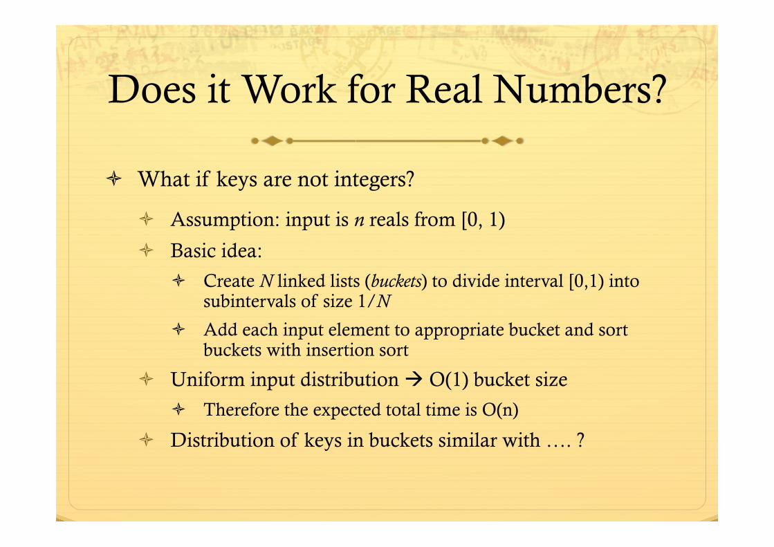
Does it Work for Real Numbers?

ò  What if keys are not integers?

ò  Assumption: input is n reals from [0, 1)

ò  Basic idea:

ò  Create N linked lists (buckets) to divide interval [0,1) into subintervals of size 1/N

ò  Add each input element to appropriate bucket and sort buckets with insertion sort

ò  Uniform input distribution à O(1) bucket size

ò  Therefore the expected total time is O(n)

ò  Distribution of keys in buckets similar with …. ?

Radix Sort

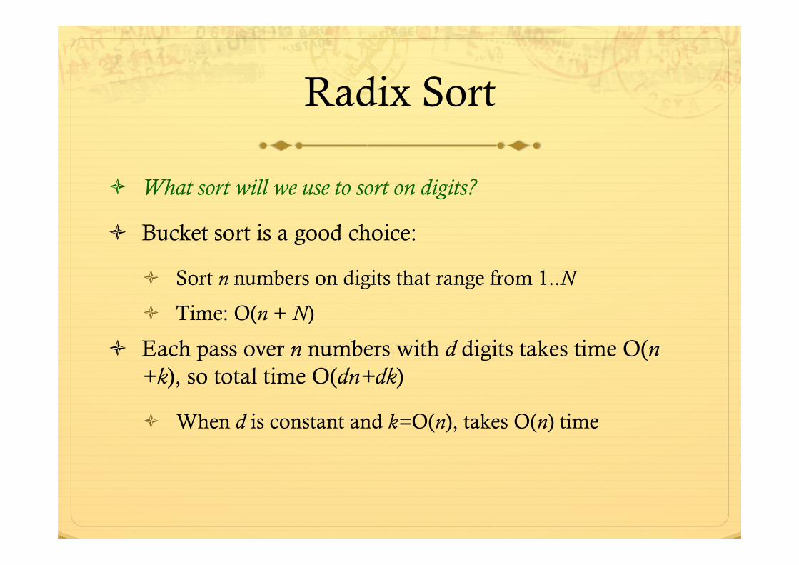
ò  What sort will we use to sort on digits?

ò  Bucket sort is a good choice:

ò  Sort n numbers on digits that range from 1..N

ò  Time: O(n + N)

ò  Each pass over n numbers with d digits takes time O(n+k), so total time O(dn+dk)

ò  When d is constant and k=O(n), takes O(n) time

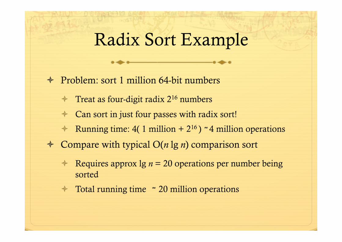
Radix Sort Example

ò  Problem: sort 1 million 64-bit numbers

ò  Treat as four-digit radix 216 numbers

ò  Can sort in just four passes with radix sort!

ò  Running time: 4( 1 million + 216 ) ≈ 4 million operations

ò  Compare with typical O(n lg n) comparison sort

ò  Requires approx lg n = 20 operations per number being sorted

ò  Total running time ≈ 20 million operations

Radix Sort

ò  In general, radix sort based on bucket sort is

ò  Asymptotically fast (i.e., O(n))

ò  Simple to code

ò  A good choice

ò  Can radix sort be used on floating-point numbers?

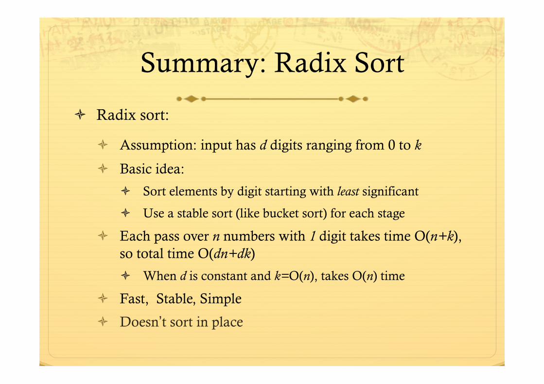
Summary: Radix Sort

ò  Radix sort:

ò  Assumption: input has d digits ranging from 0 to k

ò  Basic idea:

ò  Sort elements by digit starting with least significant

ò  Use a stable sort (like bucket sort) for each stage

ò  Each pass over n numbers with 1 digit takes time O(n+k), so total time O(dn+dk)

ò  When d is constant and k=O(n), takes O(n) time

ò  Fast, Stable, Simple

ò  Doesn’t sort in place

35

Multiway Tries

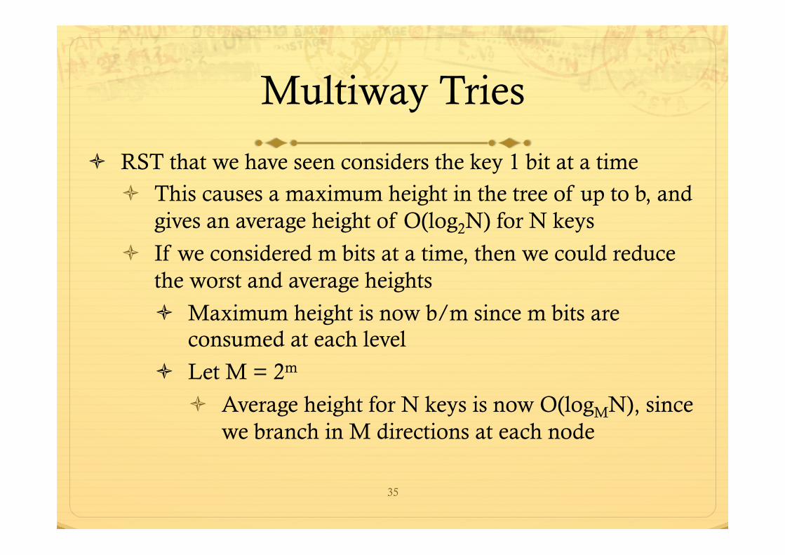
ò  RST that we have seen considers the key 1 bit at a time ò  This causes a maximum height in the tree of up to b, and

gives an average height of O(log2N) for N keys

ò  If we considered m bits at a time, then we could reduce the worst and average heights

ò  Maximum height is now b/m since m bits are consumed at each level

ò  Let M = 2m

ò  Average height for N keys is now O(logMN), since we branch in M directions at each node

36

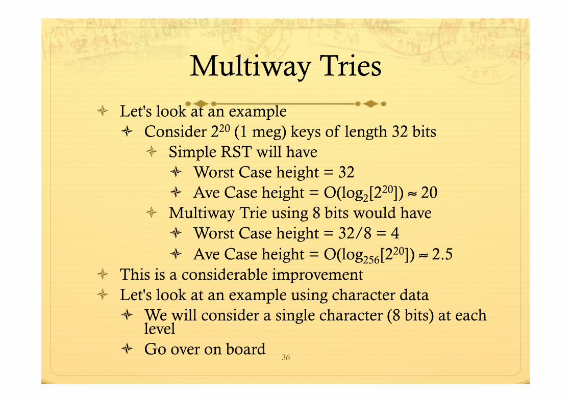
Multiway Tries ò  Let's look at an example

ò  Consider 220 (1 meg) keys of length 32 bits ò  Simple RST will have

ò  Worst Case height = 32 ò  Ave Case height = O(log2[220]) ≈ 20

ò  Multiway Trie using 8 bits would have ò  Worst Case height = 32/8 = 4 ò  Ave Case height = O(log256[220]) ≈ 2.5

ò  This is a considerable improvement ò  Let's look at an example using character data

ò  We will consider a single character (8 bits) at each level

ò  Go over on board

37

Multiway Tries

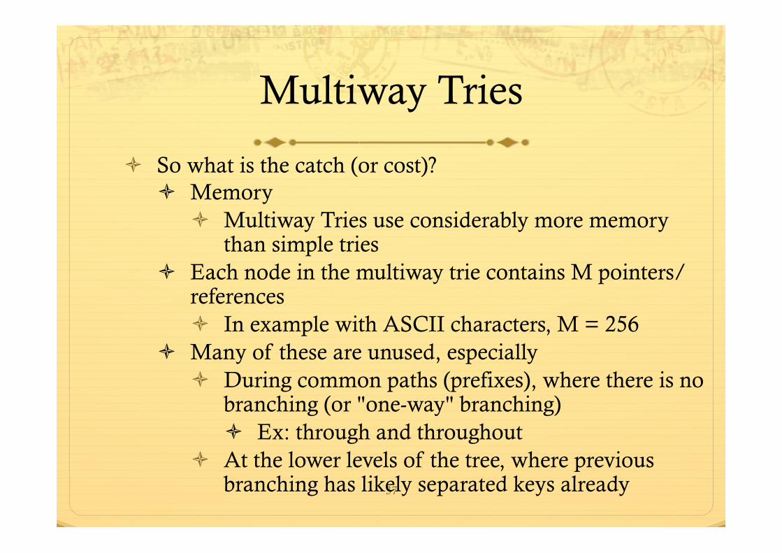
ò  So what is the catch (or cost)? ò  Memory

ò  Multiway Tries use considerably more memory than simple tries

ò  Each node in the multiway trie contains M pointers/references ò  In example with ASCII characters, M = 256

ò  Many of these are unused, especially ò  During common paths (prefixes), where there is no

branching (or "one-way" branching) ò  Ex: through and throughout

ò  At the lower levels of the tree, where previous branching has likely separated keys already

38

Patricia Trees

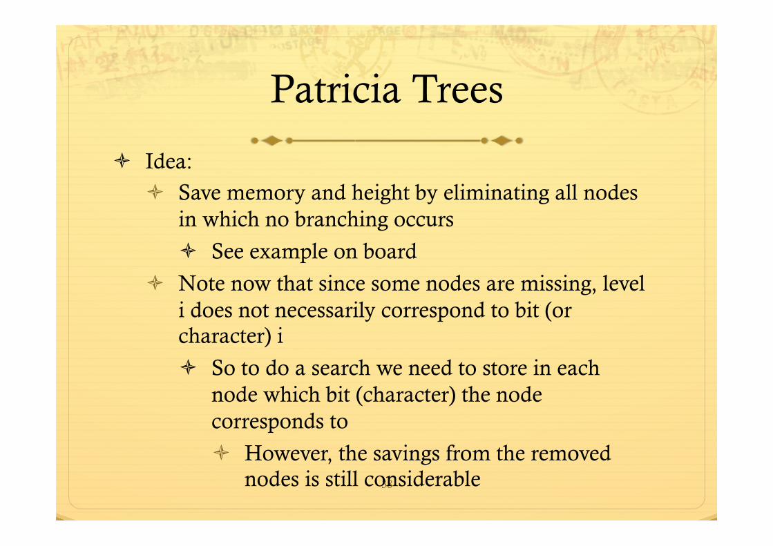
ò  Idea: ò  Save memory and height by eliminating all nodes

in which no branching occurs

ò  See example on board

ò  Note now that since some nodes are missing, level i does not necessarily correspond to bit (or character) i

ò  So to do a search we need to store in each node which bit (character) the node corresponds to

ò  However, the savings from the removed nodes is still considerable

39

Patricia Trees

ò  Also, keep in mind that a key can match at every character that is checked, but still not be actually in the tree ò  Example for tree on board:

ò  If we search for TWEEDLE, we will only compare the T**E**E

ò  However, the next node after the E is at index 8. This is past the end of TWEEDLE so it is not found

ò  Run-time? ò  Similar to those of RST and Multiway Trie,

depending on how many bits are used per node

40

Patricia Trees

ò  So Patricia trees

ò  Reduce tree height by removing "one-way" branching nodes

ò  Text also shows how "upwards" links enable us to use only one node type

ò  TEXT VERSION makes the nodes homogeneous by storing keys within the nodes and using "upwards" links from the leaves to access the nodes

ò  So every node contains a valid key. However, the keys are not checked on the way "down" the tree – only after an upwards link is followed

ò  Thus Patricia saves memory but makes the insert rather tricky, since new nodes may have to be inserted between other nodes

ò  See text

PATRICIA TREE

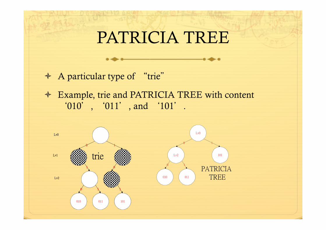
ò  A particular type of “trie”

ò  Example, trie and PATRICIA TREE with content ‘010’, ‘011’, and ‘101’.

010 011 101

1

0

1

0

1

0 1

Lv0

Lv1

Lv2

trie

Lv0

Lv2 101

011010

10

10

PATRICIA TREE

010 011 101

1

0

1

0

1

0 1

Lv0

Lv1

Lv2

trie

PATRICIA TREE

ò  Therefore, PATRICIA TREE will have the following attributes in its internal nodes:

ò  Index bit (check bit)

ò  Child pointers (each node must contain exactly 2 children)

ò  On the other hand, leave nodes must be storing actual content for final comparison

SISTRING

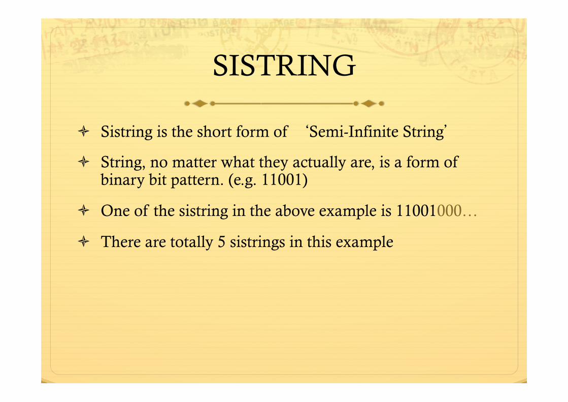
ò  Sistring is the short form of ‘Semi-Infinite String’

ò  String, no matter what they actually are, is a form of binary bit pattern. (e.g. 11001)

ò  One of the sistring in the above example is 11001000…

ò  There are totally 5 sistrings in this example

SISTRING

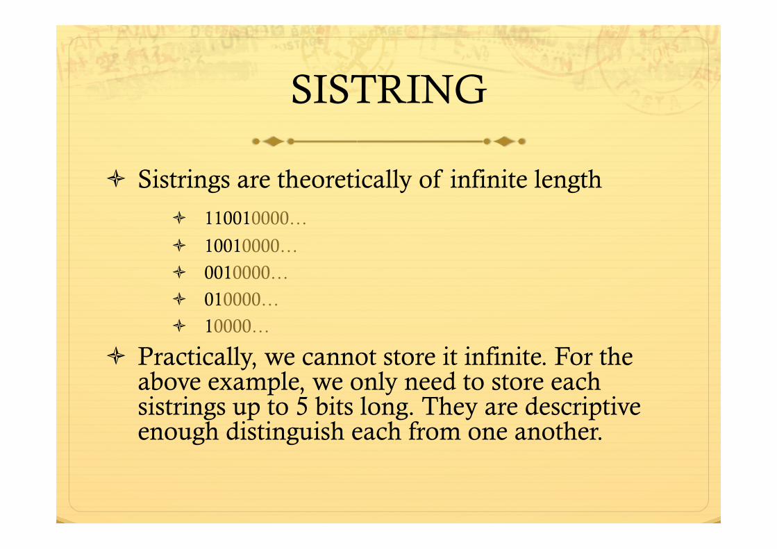
ò  Sistrings are theoretically of infinite length ò  110010000…

ò  10010000…

ò  0010000…

ò  010000…

ò  10000…

ò  Practically, we cannot store it infinite. For the above example, we only need to store each sistrings up to 5 bits long. They are descriptive enough distinguish each from one another.

SISTRING

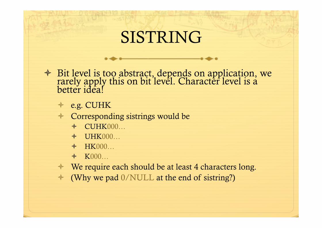
ò  Bit level is too abstract, depends on application, we rarely apply this on bit level. Character level is a better idea!

ò  e.g. CUHK ò  Corresponding sistrings would be

ò  CUHK000… ò  UHK000… ò  HK000… ò  K000…

ò  We require each should be at least 4 characters long. ò  (Why we pad 0/NULL at the end of sistring?)

SISTRING (USAGE)

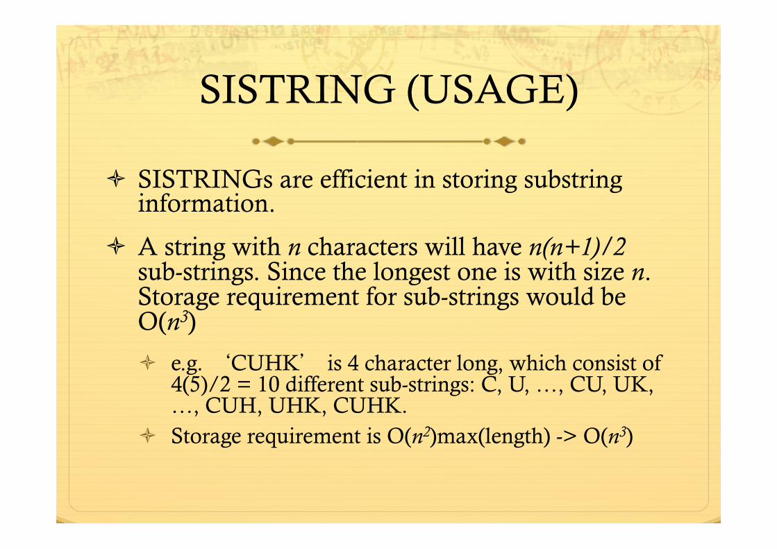
ò  SISTRINGs are efficient in storing substring information.

ò  A string with n characters will have n(n+1)/2 sub-strings. Since the longest one is with size n. Storage requirement for sub-strings would be O(n3)

ò  e.g. ‘CUHK’ is 4 character long, which consist of 4(5)/2 = 10 different sub-strings: C, U, …, CU, UK, …, CUH, UHK, CUHK.

ò  Storage requirement is O(n2)max(length) -> O(n3)

SISTRING (USAGE)

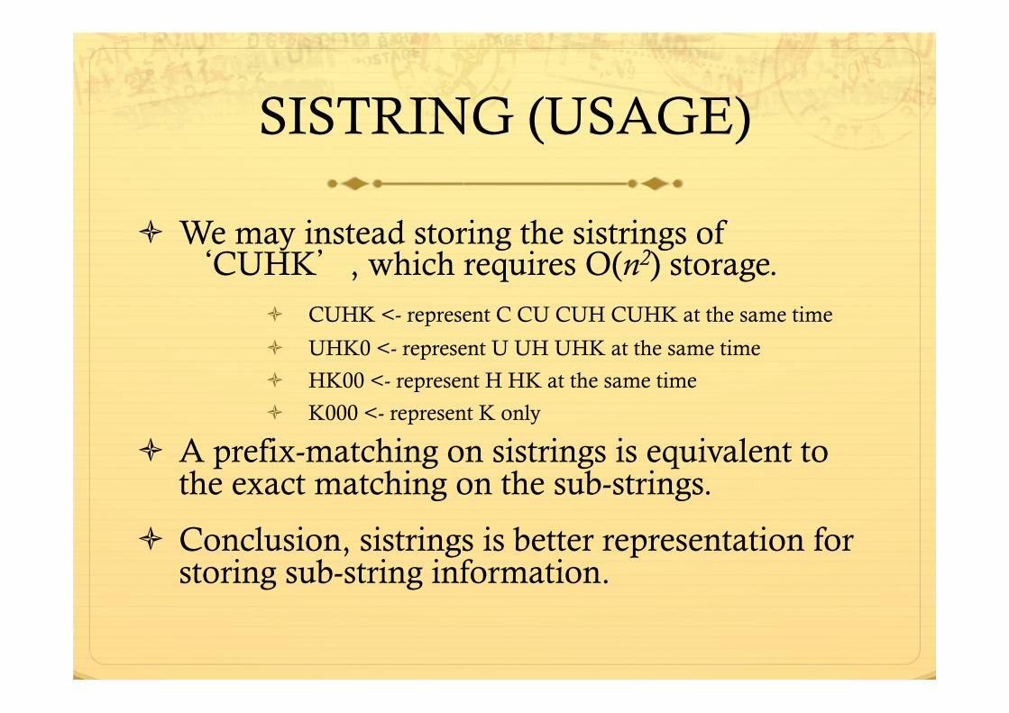
ò  We may instead storing the sistrings of ‘CUHK’, which requires O(n2) storage.

ò  CUHK <- represent C CU CUH CUHK at the same time

ò  UHK0 <- represent U UH UHK at the same time

ò  HK00 <- represent H HK at the same time

ò  K000 <- represent K only

ò  A prefix-matching on sistrings is equivalent to the exact matching on the sub-strings.

ò  Conclusion, sistrings is better representation for storing sub-string information.

PAT Tree

ò  Now it is time for PAT Tree again

ò  PAT Tree is a PATRICIA TREE store every sistrings of a document

ò  What if the document is now contain simply ‘CUHK’?

ò  We like character at this moment, but PATRICIA is working on bits, therefore, we have to know the bit pattern of each sistrings in order to know the actual figure of the PAT tree result

ò  It looks frustrating for even small example, but it is how PAT tree works!

PAT Tree (Example)

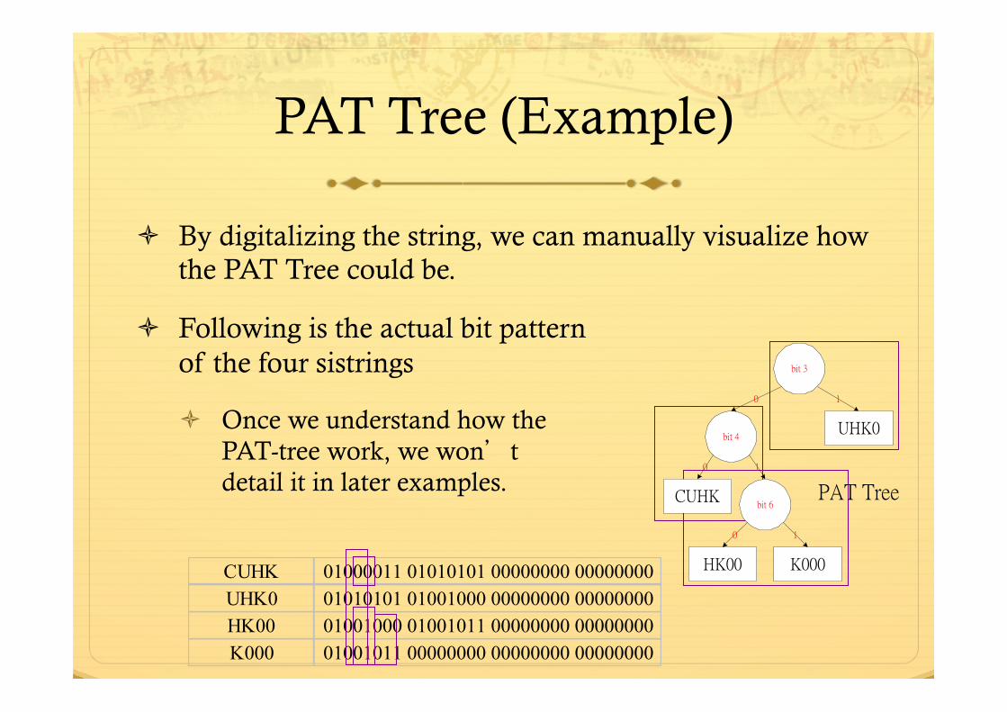
ò  By digitalizing the string, we can manually visualize how the PAT Tree could be.

ò  Following is the actual bit pattern of the four sistrings

ò  Once we understand how the PAT-tree work, we won’t detail it in later examples.

CUHK 01000011 01010101 00000000 00000000UHK0 01010101 01001000 00000000 00000000HK00 01001000 01001011 00000000 00000000K000 01001011 00000000 00000000 00000000

bit 3

bit 4

bit 6

10

10

PAT Tree

UHK0

K000HK00

CUHK

0 1

PAT Tree

ò  In a document, we don’t view it as a packed string of characters. A document consist of words. e.g. “Hello. This is a simple document.”

ò  In this case, sistrings can be applied in ‘document level’; the document is treated as a big string, we may tokenize it word-by-word, instead of character-by-character.

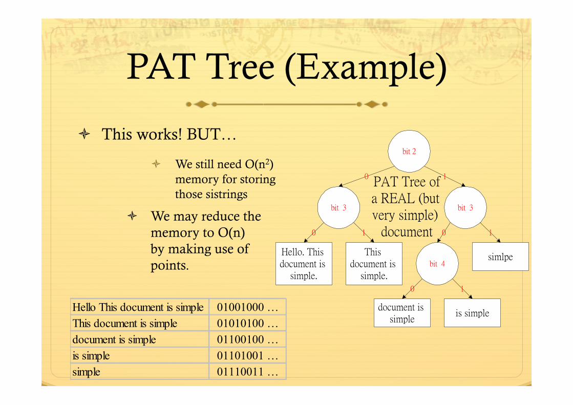
PAT Tree (Example)

ò  This works! BUT…

ò  We still need O(n2) memory for storing those sistrings

ò  We may reduce the memory to O(n) by making use of points.

Hello This document is simple 01001000 …This document is simple 01010100 …document is simple 01100100 …is simple 01101001 …simple 01110011 …

bit 2

bit 3

bit 4

10

00

PAT Tree ofa REAL (but very simple)

document

simlpe

is simpledocument is

simple

Hello. This document is

simple.

0 1

bit 3

This document is

simple.

11

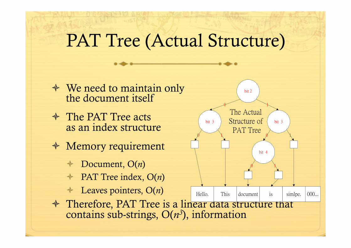
PAT Tree (Actual Structure)

ò  We need to maintain only the document itself

ò  The PAT Tree acts as an index structure

ò  Memory requirement

ò  Document, O(n) ò  PAT Tree index, O(n)

ò  Leaves pointers, O(n)

ò  Therefore, PAT Tree is a linear data structure that contains sub-strings, O(n3), information

bit 2

bit 3

bit 4

10

00

The Actual Structure of PAT Tree

0 1

bit 3

11

simlpe.isdocumentHello. This 000...

Structure modification

ò  We can see that node structure for internal node and leave node are not the same

ò  tree will be more flexible if their nodes are generic (have a universal node structure)

ò  Trade off: generic node structure will enlarge the individual node size

ò  But.. ò  Memory are cheap now

ò  Even the low end computer can support hundreds MB of RAM

ò  The modified tree is still a O(n) structure

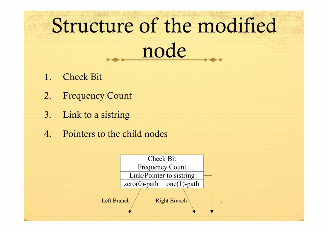
Structure of the modified node

1.  Check Bit

2.  Frequency Count

3.  Link to a sistring

4.  Pointers to the child nodes

Check Bit

zero(0)-path one(1)-path

Left Branch .Right Branch .

Frequency CountLink/Pointer to sistring

Conclusion

ò  PAT tree is a O(n) data structure for document indexing

ò  PAT tree is good for solving sub-string matching problem

ò  Chinese PAT tree has sistrings in sentence level. Frequency count is introduced to overcome the duplicate sistrings problem

ò  On generalizing the node structure, the modified version increase the pat tree capability for varies applications

Data Structures and Algorithms - Vilniaus …algis/dsax/Data-structures-5.pdfData Structures and...

Documents

Transcript of Data Structures and Algorithms - Vilniaus …algis/dsax/Data-structures-5.pdfData Structures and...