Data Set: Apartment Rents (in ascending order) Data Set: Apartment Rents.
17
445 615 430 590 435 600 460 600 440 615 440 440 440 525 425 445 575 445 450 450 465 450 525 450 450 460 435 460 465 480 450 470 490 472 475 475 500 480 570 465 600 485 580 470 490 500 549 500 500 480 570 515 450 445 525 535 475 550 480 510 510 575 490 435 600 435 445 435 430 440 425 430 430 435 435 435 435 435 440 440 440 440 440 445 445 445 445 445 450 450 450 450 450 450 450 460 460 460 465 465 465 470 470 472 475 475 475 480 480 480 480 485 490 490 490 500 500 500 500 510 510 515 525 525 525 535 549 550 570 570 575 575 580 590 600 600 600 600 615 615
-
Upload
milton-lynch -
Category
Documents
-
view
237 -
download
0
Transcript of Data Set: Apartment Rents (in ascending order) Data Set: Apartment Rents.
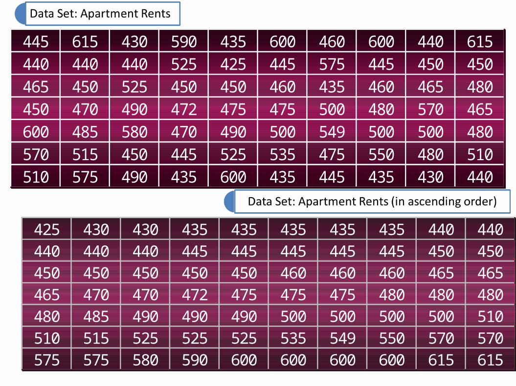
445 615 430 590 435 600 460 600 440 615440 440 440 525 425 445 575 445 450 450465 450 525 450 450 460 435 460 465 480450 470 490 472 475 475 500 480 570 465600 485 580 470 490 500 549 500 500 480570 515 450 445 525 535 475 550 480 510510 575 490 435 600 435 445 435 430 440
425 430 430 435 435 435 435 435 440 440440 440 440 445 445 445 445 445 450 450450 450 450 450 450 460 460 460 465 465465 470 470 472 475 475 475 480 480 480480 485 490 490 490 500 500 500 500 510510 515 525 525 525 535 549 550 570 570575 575 580 590 600 600 600 600 615 615
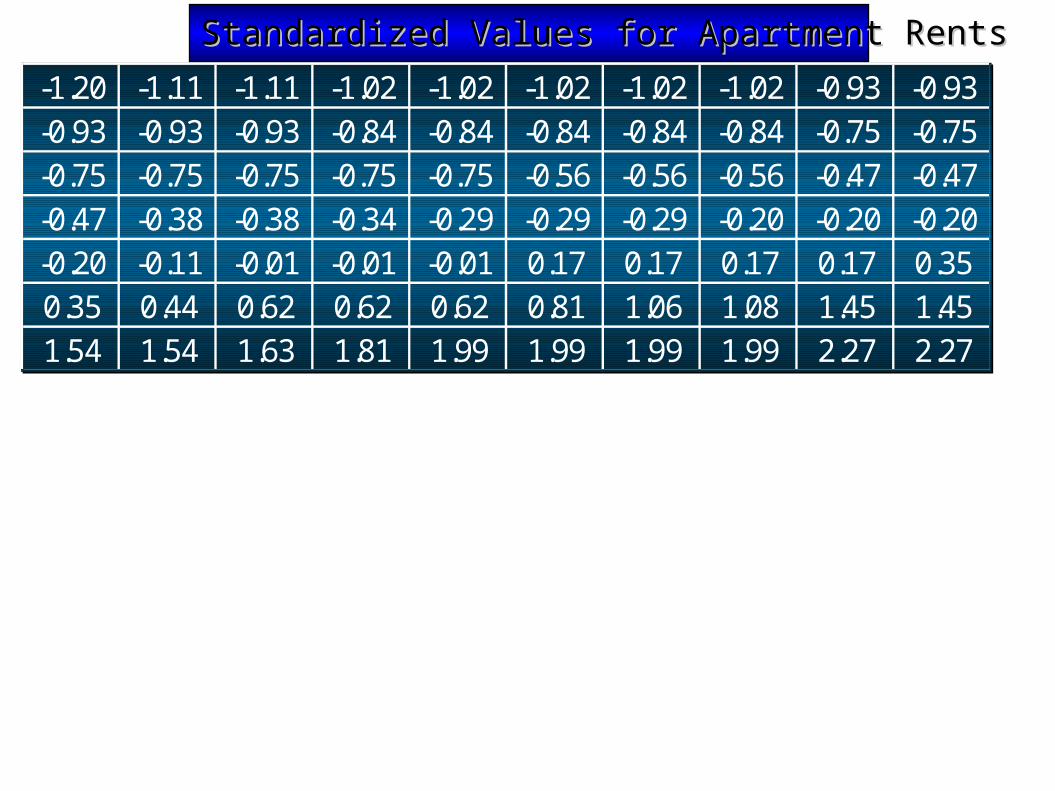
-1.20 -1.11 -1.11 -1.02 -1.02 -1.02 -1.02 -1.02 -0.93 -0.93-0.93 -0.93 -0.93 -0.84 -0.84 -0.84 -0.84 -0.84 -0.75 -0.75-0.75 -0.75 -0.75 -0.75 -0.75 -0.56 -0.56 -0.56 -0.47 -0.47-0.47 -0.38 -0.38 -0.34 -0.29 -0.29 -0.29 -0.20 -0.20 -0.20-0.20 -0.11 -0.01 -0.01 -0.01 0.17 0.17 0.17 0.17 0.350.35 0.44 0.62 0.62 0.62 0.81 1.06 1.08 1.45 1.451.54 1.54 1.63 1.81 1.99 1.99 1.99 1.99 2.27 2.27
Standardized Values for Apartment RentsStandardized Values for Apartment Rents
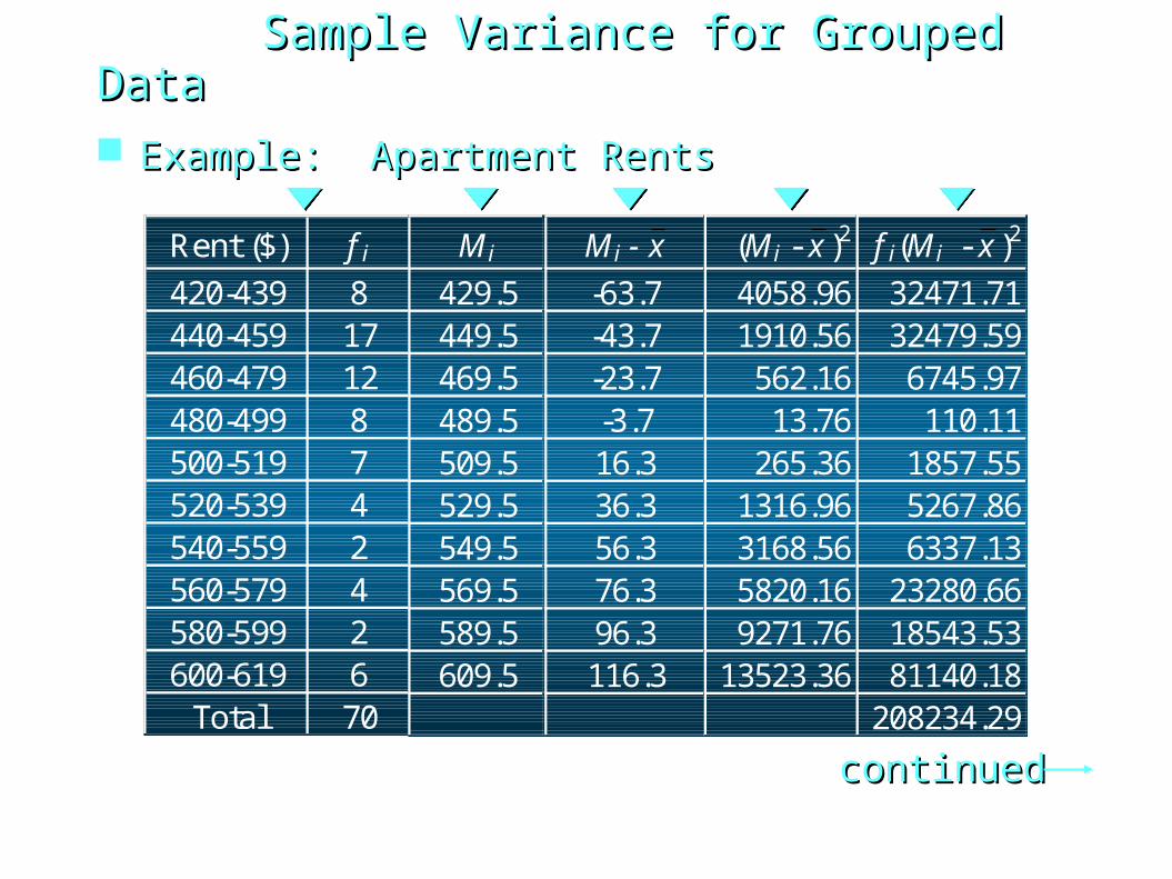
Sample Variance for Grouped DataSample Variance for Grouped Data
continuedcontinued
Rent ($) f i
420-439 8440-459 17460-479 12480-499 8500-519 7520-539 4540-559 2560-579 4580-599 2600-619 6
Total 70
M i
429.5449.5469.5489.5509.5529.5549.5569.5589.5609.5
M i - x
-63.7-43.7-23.7-3.716.336.356.376.396.3116.3
(M i - x )2
4058.961910.56562.1613.76
265.361316.963168.565820.169271.76
13523.36
f i(M i - x )2
32471.7132479.596745.97110.11
1857.555267.866337.13
23280.6618543.5381140.18
208234.29
Example: Apartment RentsExample: Apartment Rents
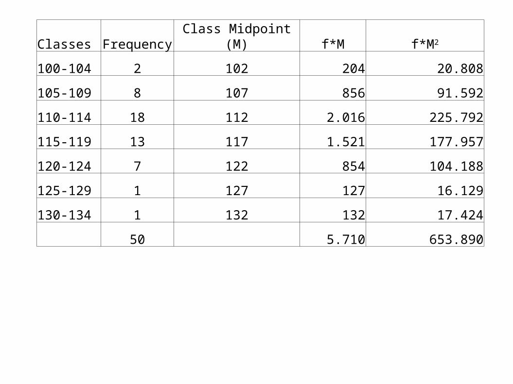
Classes Frequency Class Midpoint (M) f*M f*M2
100-104 2 102 204 20.808
105-109 8 107 856 91.592
110-114 18 112 2.016 225.792
115-119 13 117 1.521 177.957
120-124 7 122 854 104.188
125-129 1 127 127 16.129
130-134 1 132 132 17.424
50 5.710 653.890
A student scored 65 on statistics test that had a mean of 50 and a standard deviation of 10, she scored 30 on history test with a mean of 25 and a standard deviation of 5. Compare her relative positions on the two tests
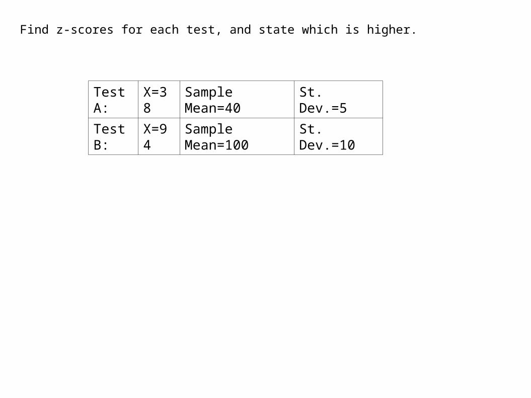
Find z-scores for each test, and state which is higher.
Test A: X=38 Sample Mean=40 St. Dev.=5
Test B: X=94 Sample Mean=100 St. Dev.=10

Which score has the highest relative position.
A X=12 Sample Mean=10 St. Dev.=4
B X=170 Sample Mean=120 St. Dev.=32
C X=180 Sample Mean=60 St. Dev.=8

The mean price of houses in a certain neighborhood is 50,000 USD and standard deviation is 10,000 USD. Find the price range for which at least 75% of the houses will sell.
A survey of local companies found that the mean amount of travel allowances for executives was 0.25 USD per mile. The standard deviation was 0.02 USD. Using Chebyshev`s Theorem find the minimum percentage of the data values that will fall between 0.20 USD and 0.30 USD.

Example: Apartment Rents (TL)
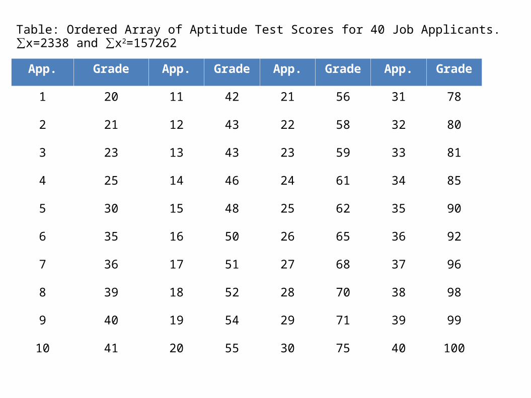
App. Grade App. Grade App. Grade App. Grade
1 20 11 42 21 56 31 78
2 21 12 43 22 58 32 80
3 23 13 43 23 59 33 81
4 25 14 46 24 61 34 85
5 30 15 48 25 62 35 90
6 35 16 50 26 65 36 92
7 36 17 51 27 68 37 96
8 39 18 52 28 70 38 98
9 40 19 54 29 71 39 99
10 41 20 55 30 75 40 100
Table: Ordered Array of Aptitude Test Scores for 40 Job Applicants.∑x=2338 and ∑x2=157262
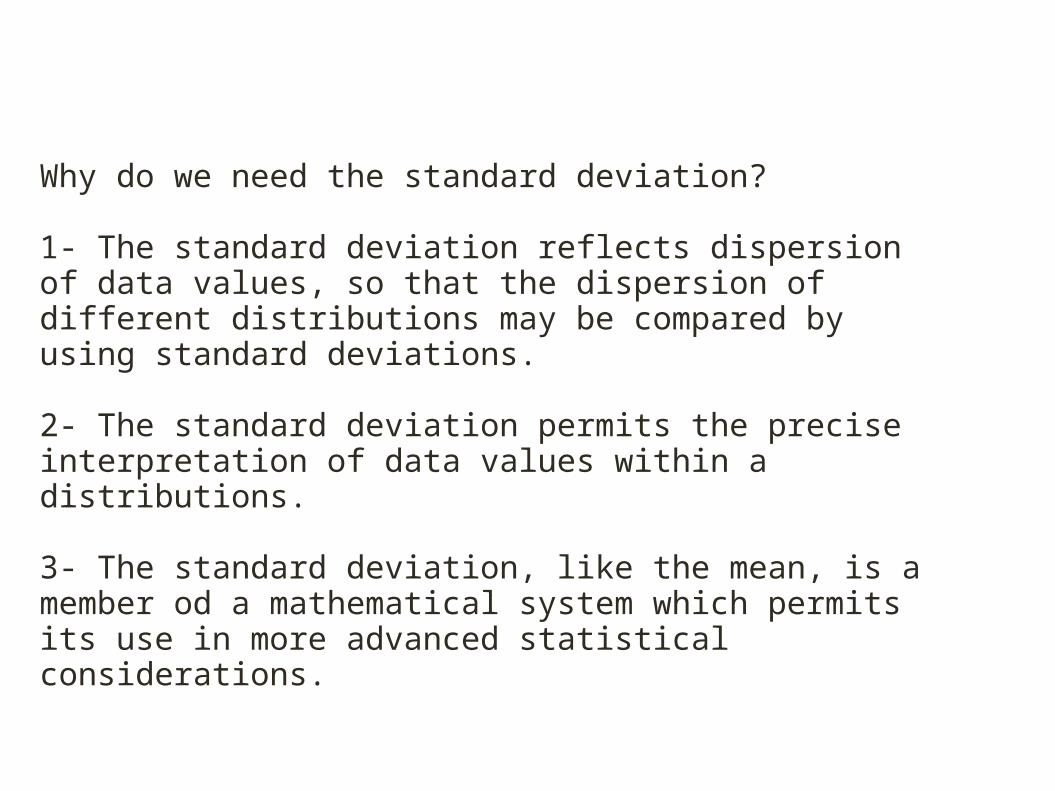
Why do we need the standard deviation?
1- The standard deviation reflects dispersion of data values, so that the dispersion of different distributions may be compared by using standard deviations.
2- The standard deviation permits the precise interpretation of data values within a distributions.
3- The standard deviation, like the mean, is a member od a mathematical system which permits its use in more advanced statistical considerations.
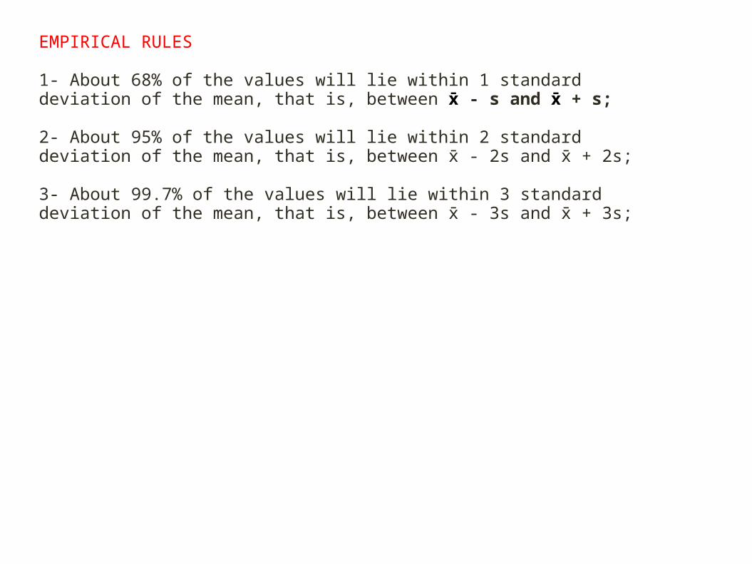
EMPIRICAL RULES
1- About 68% of the values will lie within 1 standard deviation of the mean, that is, between x̄� - s and x̄� + s;
2- About 95% of the values will lie within 2 standard deviation of the mean, that is, between x@ - 2s and x@ + 2s;
3- About 99.7% of the values will lie within 3 standard deviation of the mean, that is, between x@ - 3s and x@ + 3s;
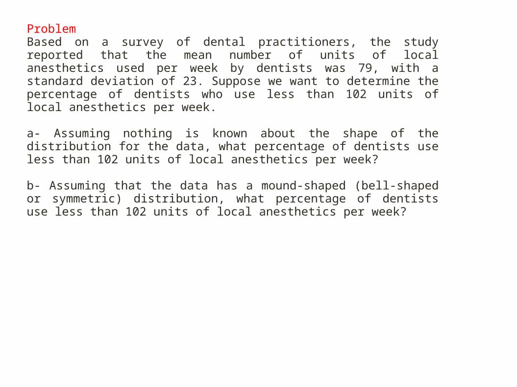
ProblemBased on a survey of dental practitioners, the study reported that the mean number of units of local anesthetics used per week by dentists was 79, with a standard deviation of 23. Suppose we want to determine the percentage of dentists who use less than 102 units of local anesthetics per week.
a- Assuming nothing is known about the shape of the distribution for the data, what percentage of dentists use less than 102 units of local anesthetics per week?
b- Assuming that the data has a mound-shaped (bell-shaped or symmetric) distribution, what percentage of dentists use less than 102 units of local anesthetics per week?
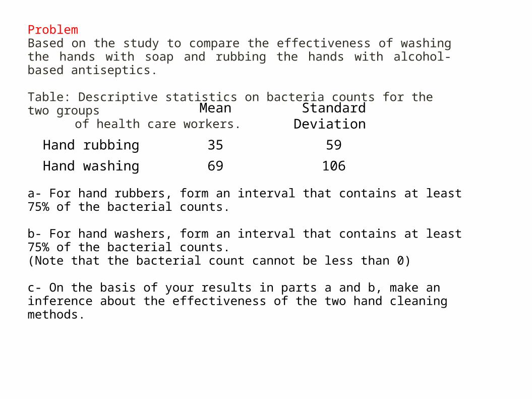
ProblemBased on the study to compare the effectiveness of washing the hands with soap and rubbing the hands with alcohol-based antiseptics.
Table: Descriptive statistics on bacteria counts for the two groups of health care workers.
Mean Standard Deviation
Hand rubbing 35 59
Hand washing 69 106
a- For hand rubbers, form an interval that contains at least 75% of the bacterial counts.
b- For hand washers, form an interval that contains at least 75% of the bacterial counts. (Note that the bacterial count cannot be less than 0)
c- On the basis of your results in parts a and b, make an inference about the effectiveness of the two hand cleaning methods.