Data Science for Planetary Science - indico.lal.in2p3.fr fileData Science for Planetary Science...

Data Science for Planetary Science

Frédéric SchmidtCenter for Data Science

Paris-Saclay

Planetary Science• Planetary formation

• From disk to (exo)planets

• Meteorites, comets

Planetary Science

• Planetary bodies

• Interior

• Surface

• Atmosphere

• Ionosphere

Planetary Science

• Planetary bodies

• Interior

•Surface

•Atmosphere

• Ionosphere

Remote sensing : imagery

Big scientific questions

• Geologic evolution (tectonic, volcanic, ...)

• Climate evolution (climate change, escape, ...)

• Habitability (origin of life, human exploration)

Big scientific questions

• Geologic evolution (tectonic, volcanic, ...)

• Climate evolution (climate change, escape, ...)

• Habitability (origin of life, human exploration)

? ?

Raw data

• Mars Express (ESA, launched in 2003) : ~50 Tb

• Mars Reconnaissance Orbiter (NASA, launched in 2005) : ~200 Tb

Calibrated data

• Increase factor : ~10

Huge amount of data

• How to treat the data ?

• How to represent the scientific results (in a global map) ?

Franquin, Gaston Lagaffe

Large volume products

• High resolution spectra

• High resolution images

• Hyperpectral images

• Multi-angular hyperspectral images



•High resolution images

• Hyperpectral images


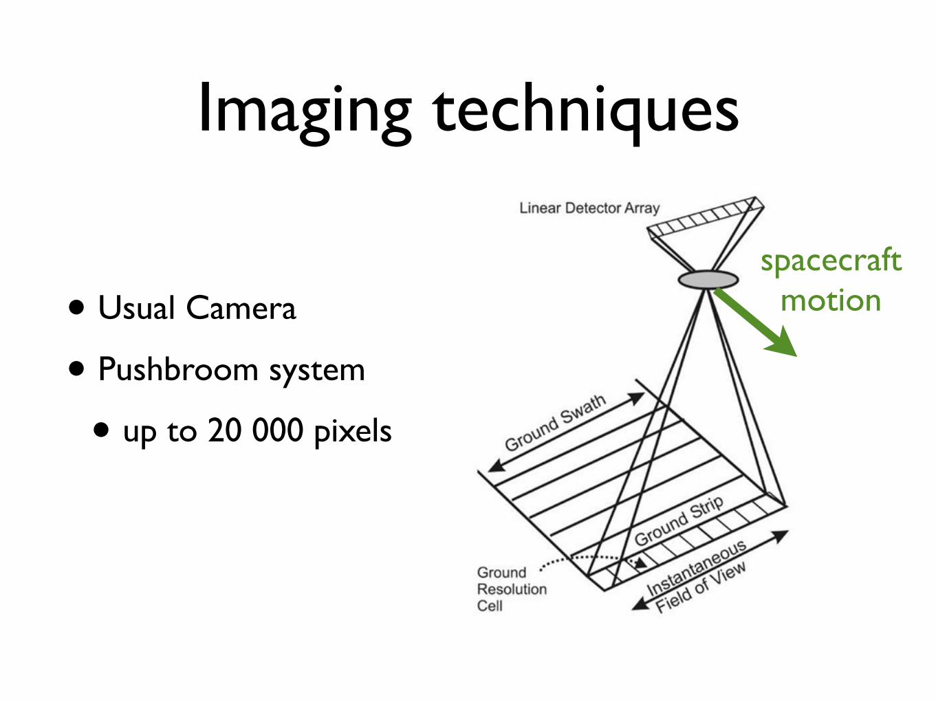
Imaging techniques

• Usual Camera

• Pushbroom system

• up to 20 000 pixels

spacecraft motion

Examples of high resolution images datasets

• MOC (Mars Global Surveyor, NASA)

• HRSC (Mars Express, ESA)

• ISS (Cassini, NASA)

• HiRISE (Mars Reconnaissance Orbiter, NASA)

• ...

Neukum et al., 2004

Malin and Edgett, 2000

Porco et al., 2004

McEwen et al., 2007

Tools for large dataset treatment:

1. global scale mosaic visualisation

2. stereoscopy to create DEM

3. change detection (crater, dust devils, dune, ...)

4. automatic feature identification

Data Science Challenges for images

1. Scientific data visualisation

• Google Mars

• MapAPlanet

• JMars,...

• Limitations:

• no scientific data

• not complete

• Slow

http://jmars.asu.edu/

http://www.mapaplanet.org/

http://www.google.com/mars/

http://jmars.asu.edu

http://jmars.asu.edu

http://www.mapaplanet.org

http://www.mapaplanet.org



1. Data visualisation project

• Web based approach

• 3D and GIS oriented

• C. Marmo (GEOPS/IAS/OSUPS)

2. Digital Elevation Model

• Stereoscopy

• based on image correlation

• Limitations:

• Very slow

• Uncertainties ?

3. Change detection

• HiRISE (august 2011)

• Flow

• Summer (~30°S)

• Liquid water ?

McEwen et al., 2011

4. Feature detection

• Automatic crater counting

• on images

• on DEM

• Limitations:

• very slow

• accuracy

Stepinski et al., 2009

Author's personal copy

Fig. 3. Craters identified by the AutoCrat system in the Terra Cimmeria 1 site (top left), the Terra Cimmeria 2 site (bottom left), the Terra Cimmeria 3 site (top right), and theTerra Cimmeria 4 site (bottom right). The background shows the topography; high-to-low areas are depicted by dark-to-light grays.

Fig. 4. Craters identified by the AutoCrat system in the Hesperia Planum site (left) and the Sinai Planum site (right). The background shows the topography; high-to-low areasare depicted by dark-to-light grays.

Fig. 5. Craters identified by the AutoCrat system in the Amazonis Planitia site (left) and the Olympica Fossae site (right). The background shows the topography; high-to-lowareas are depicted by dark-to-light grays.

82 T.F. Stepinski et al. / Icarus 203 (2009) 77–87

Urbach et al., 2009

Data Science Challenges for images

• Data treatment (DEM)

• Data mining (change detection, feature identification)

• How to represent the data (global map, time) ?



• High resolution images

•Hyperpectral images


Contribution:•atmosphere•surface

Visible and Near-IR signal

Wavelength (microns)

Wavelength (microns)

Refl

ecta

nce

Typical soil

Ices

CO2

H2O

Atmospheric features

Refl

ecta

nce

Imaging spectrometer

• Hyperspectral image

• Maps surface/atmosphere properties> 100 wavelengths

CO2

H2O

Examples of hyperspectral datasets

• OMEGA (Mars Express, ESA)

• VIRTIS (Venus Express, ESA)

• VIMS (Cassini, NASA)

• CRISM (Mars Reconnaissance Orbiter, NASA)

• ...

Bibring et al., 2004

Drossart et al., 2007

Brown et al., 2004

Murchie et al., 2007

• Detection

• band ratios, wavelets, linear unmixing

• Quantification

• radiative transfer inversion

Data Science Challengesfor hyperspectral images

•Detection


• Quantification



Detection using Band ratio

• Very Fast

• Limitations:

• superposition of bands

• angular effects

role in spectral analysis, briefly describe the CRISM andOMEGA data sets, discuss the methodology and results ofthe summary product validation process, and conclude witha summary and review the limitations associated with thesedata products.

2. Spectral Parameters2.1. Background

[5] The idea of utilizing parameters to analyze spectraldata has been used with success in past analyses of spectraldata from Mars [e.g., Bell et al., 2000;Murchie et al., 2000].The concept rests on the idea that a given spectral featurecan be captured by a single parameter value, which iscalculated by applying an algorithm using combinationsof spectral bands to the data. Each parameter is designedwith a specific rationale in mind; ideally, to capture spectralfeatures unique to a specific mineralogy. Typically theparameter value is then mapped across a region toassess spatial variations of the spectral feature, which, inturn, are interpreted as spatial variations of the associatedmineralogy.[6] The CRISM summary products will be derived from

reflectances in key wavelengths and will make use of manyparameters used in previous studies such as single bandreflectances, reflectance ratios, spectral slope, and depths ofmineralogic or gaseous absorptions. In this work, reflec-tance is represented by the symbol R. Surface parameterswill be derived from reflectances that have undergonephotometric, thermal, and atmospheric corrections; atmo-spheric parameters will be derived from reflectances under-

going only a simple photometric correction to normalizeobservations to a standard viewing geometry.[7] Figure 1 demonstrates examples of some of the most

common spectral parameters, including those mentionedabove. In Figure 1, the reflectance at the wavelengthindicated by the point labeled 1 (i.e., at l1) is representedas R1. Spectral slope refers to the slope of the spectralcontinuum (the general shape of a spectrum in the absenceof specific absorptions) and is represented as the changein reflectance over a given wavelength interval. Thegeneral representation of spectral slope is DR/Dl; in theexample spectrum of Figure 1, the spectral slope is foundby (R1 ! R2)/(l1 ! l2). For absorptions, the depth ofthe absorption, or band depth, is generally represented as1 ! Rl/R*l, where Rl is the reflectance at the wavelengthof the center of the absorption, and R*l is the interpolatedcontinuum reflectance at the same wavelength. Thecontinuum level is created from a linear fit between twowavelengths from either side of the absorption that are at leastlocal continuum levels. Using the difference of this ratiofrom 1 is a favored convention because it results in largerband depths for deeper absorptions. In the Figure 1 example,the band depth is 1 ! RC/RC*, where RC is the reflectance atthe center of the band, and RC* is derived from the continuumfit across the band and is equal to (a*RS + b*RL), where a =1 ! b and b = (lC ! lS)/(lL ! lS). Generally, band depthscales with the abundance of the absorbing mineral, thoughcompounding factors such as particle size and albedo alsohave an effect [Clark and Roush, 1984].

2.2. CRISM Spectral Parameters

[8] The spectral parameters that will be used with theCRISM data are designed specifically for the CRISMwavelength regime. On the basis of a priori expectationsof the composition of Mars, we began with a set of35 parameters that primarily focused on broad maficfeatures expected in surface spectra and narrow hydrationfeatures expected in spectra from both the surface and theatmosphere. We then tested and evaluated these initialparameters using OMEGA data.[9] Detailed analysis revealed that much of the spectral

diversity of Mars was captured by a number of the originalparameters but also that several parameters failed to showrelevant variations as anticipated, and that some featuresidentified with the full OMEGA spectral resolution were notcaptured at all (e.g., the sulfates and phyllosilicates reportedby Bibring et al. [2005], Gendrin et al. [2005], andLangevin et al. [2005b]). Thus parameter formulations werereworked; some parameters were eliminated, and newparameters were added. Table 1 represents the CRISMsummary products as defined at the time of publication,along with their formulations and rationale, refined accord-ing to the results of our validation efforts and the OMEGAmission itself. The outcome is a robust set of parameterscapable of capturing the known atmospheric constituentsand diverse surface mineralogy of Mars, as well as inter-esting atmospheric constituents and mineralogy yet to bedetected at the planet.[10] As the parameters in Table 1 are derived from

multispectral data, the level of discrimination is limited.Most parameters have been designed to identify mineralclasses rather than mineralogic species. There are 33 param-

Figure 1. An explanation of some of the most commonspectral parameters using an idealized spectrum. The solidline is an idealized spectrum with an absorption bandsuperimposed on a sloped continuum. In the aboveexample, the reflectance at the wavelength indicated bythe point labeled 1 (i.e., at l1) is represented as R1. Spectralslope is found by (R1 ! R2)/(l1 ! l2). Band depth is foundby 1 ! RC/RC*, where the point labeled C indicates thecenter of the absorption at lC, RC is the reflectance at thatwavelength, and RC* is derived from the continuum fitalong the dashed line and is equal to (a*RS + b*RL), wherea = 1-b and b = (lC ! lS)/(lL ! lS).

E08S14 PELKEY ET AL.: CRISM MULTISPECTRAL SUMMARY PRODUCTS

2 of 18

E08S14

Absorption depth

very small, and they might be nanocrystallinered hematite a-Fe203 or possibly maghemiteg-Fe203. Such small particles would be easilytransported, stick on most grains, and accountfor the magnetic properties of the soil measuredby the MERs (16). Ferric oxides are also de-tected in localized areas with a variety ofalbedo (such as within Terra Meridiani, VallesMarineris, or Aram Chaos).

Two types of hydrated minerals have beenidentified from OMEGA data: phyllosilicates(10, 17) (Fig. 2B) and sulfates (10, 18–20) (Fig.2C), but in only a few locations (17) (Fig. 3).Carbonate-rich areas have not been found byOMEGA, although a low concentration of car-bonate is interpreted from TES data on martiandust (21), and carbonates are recognized inmartian meteorites (22).

From their near-IR (0.8 to 2.6 mm) spectra,we infer that most of the phyllosilicate mineralsare Fe-rich (such as chamosite and nontronite),although Al-rich phyllosilicates (such as mont-morillonite) are locally dominant (17). Theseclayminerals are found in a variety of light-tonedoutcrops and scarps, primarily in rocks and soilsnorth of the Hesperian-aged Syrtis Major volcan-ic plateau, Nili Fossae, and the Marwth Vallisregions. In all these regions, phyllosilicates aremapped associated with ancient Noachian-agedsurfaces. For example, in Nili Fossae, thinNoachian-aged but unaltered mafic units restdirectly on phyllosilicate-bearing outcrops. Infor-mation from the Mars Express HRSC, the MGSMOC, and the Odyssey THEMIS images clearlyindicates that the phyllosilicates are in rocksburied by more recent deposits; the hydratedsilicate-bearing bedrock has been exposed

through erosion. The surface material of Noachi-an terrains, which are identified as being heavilycratered, does not necessarily all date from theNoachian times. Rocks of Noachian age areexposed in spots because of impact, faulting, orerosion.

In the Syrtis Major and Nili Fossae regions,phyllosilicate-rich rocks are detected in bothancient craters and material recently excavatedfrom ancient terrains beneath a later volcaniccover. These relations demonstrate that theseimpacts did not dehydrate the minerals. In con-trast, no hydrated minerals are detected in thelobate craters (thought to form by impact intovolatile-rich substrates) within the lava flowsfrom Nili Patera, which embay the ancientterrains (10). This relation suggests that miner-alization of hydrated minerals occurred beforethe emplacement of the Hesperian-aged lavasfrom Nili Patera and that these lavas areessentially water-free. In the Marwth Vallis re-gion (Fig. 4), hydrated minerals are not foundin the channel nor in its opening but rather onthe surrounding plateau and its eroded flanks.Thus, water associated with the formation ofthe channel did not lead to phyllosilicate for-mation, although this outflow was sufficient toproduce severe erosion, including exposing theancient clay-rich minerals. So far, none of themajor and minor outflow channels or the valleynetworks show evidence of hydrated minerals.

Sulfates, including Mg sulfates (such askieserite) and Ca sulfates (such as gypsum), con-stitute the second major class of hydrated min-erals mapped by OMEGA and detected by theNASA rovers (7). OMEGA has shown that thesulfate-rich areas are not restricted to the gray

hematite-rich regions detected by the MGSTES (2, 5, 6). We have detected three principaltypes of hydrated sulfate deposits: layered de-posits within Valles Marineris, extended depositsexposed from beneath younger units as in TerraMeridiani, and the dark dunes of the northernpolar cap (10, 18–20).

Sequential mineral formation. Environ-ments conducive to clay mineral formationmay have existed at or near the surface or inthe deeper subsurface. Surface or near-surfaceconditions would not require high-temperatureconditions (hydrothermal, for example). Sur-face formation of these clay minerals wouldindicate a long-lasting wet episode, with largesurface aqueous reservoirs and alkaline waterresulting from this chemical alteration, oc-curring during the Noachian.

Clay minerals could also have been formedprimarily in the subsurface, by one of the threefollowing processes: hydrothermal activity (23);cratering, supplying subsurface water (liquidand/or ice) to the impacted minerals (24); or dur-ing the cooling of the mantle, if not thoroughlydepleted of volatile compounds. These deepscenarios would not require a warm Mars tohave existed over extended time scales, andthey could have taken place even if Mars neversustained a dense atmosphere. In addition, theformation of clay minerals could have con-tinued at greater depths long after conditions atthe surface became unfavorable.

Sulfate mineral formation requires substan-tial quantities of water to account for the broaddistribution of minerals seen by OMEGA. Be-cause sulfate precipitation requireswater to evap-orate, it is essentially a surface process. For at

Fig. 1. Global mapsof pyroxene (top) andanhydrous nanophaseferric oxides (bot-tom), exhibiting theanticorrelation be-tween surface maficsand altered minerals(in the form of ferricoxides). The crateredcrust with large pyrox-ene content (top, yel-low to red) is notcovered with alteredminerals (bottom, blueto green). Conversely,the large areas with nomafics (top, blue) cor-respond to the higherconcentration of ferricoxides (bottom, red towhite).

RESEARCH ARTICLES

www.sciencemag.org SCIENCE VOL 312 21 APRIL 2006 401

on

Febr

uary

25,

200

9 w

ww

.sci

ence

mag

.org

Dow

nloa

ded

from

Pyroxene global map

Bibring et al., 2006

Bibring et al., 2006Pelkey et al., 2007Carter et al., 2014

• WAVANGLET

• correlation in a wavelet coefficient subspace

• Fast and efficient to remove angular effect

• Limitations:

• ~10 endmembers

Detection using Wavelets

Schmidt et al., Icarus 2009

Schmidt et al., IEEE TGRS 2007

SCHMIDT et al.: WAVANGLET: AN EFFICIENT SUPERVISED CLASSIFIER 1379

compound in the image, regardless of its physical properties,and and must minimize false detections.

As the SA calculation is invariant with any linear ortho-normal transformation, such as the Daubechies WT, we havethe choice to perform the SA mapping of all the pixels in thefiltered wavelet base or in the filtered spectral space. The latteris reconstructed by the inverse transform of the filtered waveletbase. The calculation of the SA is faster in the filtered waveletbase than in the complete spectral space because the dimensionsof the former are lower. We therefore choose to perform thecalculation in the filtered wavelet base.

D. Step D: Automatic Mass Classification With SAs inThis Subspace

All the parameters are now adjusted to perform the auto-mated classification. For each image and each spectrum of thereference base, a detection mask will be created. For datasetsspanning a long time range (several months to years), many pa-rameters can vary. For instance, the bad channel list can changewith time thus affecting Steps B2 and B3. If this happens, thenStep C should be adapted according to the former steps.

IV. EXPERIMENTS

We will now apply this general wavanglet method to aseries of OMEGA/MEX hyperspectral images and comparethe obtained classifications with the ones produced by twoalternative methods: BR and SFF (Section II-C1 and -C3). Wealso evaluate quantitative detection limits for H2O and CO2 icesin terms of abundance. We use synthetic spectra for this. Thispaper consists of five tests: classification accuracy, separabilitybetween classes, multiple endmembers and possible overlap-ping signatures, mass processing feasibility, and calculationtime.

A. Application of the Wavanglet Method to the Omega Dataset

We follow the four steps described in Section III to apply themethod to a collection of OMEGA/MEX images covering thepolar regions of Mars.1) Step A—Choice of Relevant “Endmembers” (Reference

Spectra): The OMEGA spectra display signatures characteris-tic of both the atmosphere and the surface. The atmosphericcontribution is due to gaseous CO2 and, depending on weatherconditions, to clouds of dust, CO2, and H2O ices. The spectraleffect of the clouds can often be neglected for a first-orderapproximation. The surface contribution is due to a mixtureof H2O ice, CO2 ice, and dust in various proportions. In theimages, we try to detect the last three compounds to whichwe attribute reference spectra (see Fig. 2). Pure H2O and CO2

are represented by synthetic spectra computed by a reflectancemodel [18] using the physical parameters listed in Table III andan optical constant measured in the laboratory [25]–[27]. Theseparameters have been chosen to be compatible with recentstudies of both south and north Martian polar regions [10], [11],[28], [29]. On the other hand, the third reference spectrum rep-resenting polar dust is extracted from a single OMEGA imagecovering the southern high latitudes by averaging all spectrawithin a relatively homogeneous region near 70! longitude

TABLE IIISYNTHETIC ENDMEMBER PARAMETERS

TABLE IVLIST OF ELIMINATED WAVELETS

Fig. 3. Representation of the selected subspace of (upper part) wavelets thatbest discriminate the endmembers (lower part). (a)–(d) Wavelets selected inscales 5 to 8. (e) Observed dust and atmosphere spectra, (f) synthetic CO2 ice,and (g) synthetic H2O ice. See Section II-B for wavelet representation.

and "77! latitude. Note that this spectrum is almost featurelessin the near-infrared range except for the 3-µm band due tothe hydration of the minerals and the absorption bands ofatmospheric CO2. Globally, the dust spectrum does not displaymuch spatial variation in this spectral range. Indeed, it is wellmixed by winds and spread over wide areas. Thus, we can as-sume that our reference spectrum is representative of most areasof both polar regions. Our Martian studies focus mainly on thetwo first endmembers while the third endmember representsspectral features that appear in the data but which are not ofinterest to us.2) Step B—Determination of the Best Subspace:Step B1—Continuum removal: We use only the last four

scales (from 5 to 8) in order to remove the contribution of thecontinuum.

Step B2—Best discrimination: We prefer the automaticthreshold method [method 3)], with norm L2 and the valuec = 2.5 to select the best subspace. This threshold criterionoptimizes the classification.

Step B3—Circularity, noise, and dead spectels: We elim-inate all wavelets containing a nonzero contribution from thelast spectel number 255.

We eliminate wavelets polluted by damaged spectels (num-ber 34, 78, and 158) with an energy criterion (D = 0.45).Table IV lists the indexes of the eliminated wavelets.

Finally, the selected subspace is formed by the 12 waveletsshown in Fig. 3 and summarized in Table V.

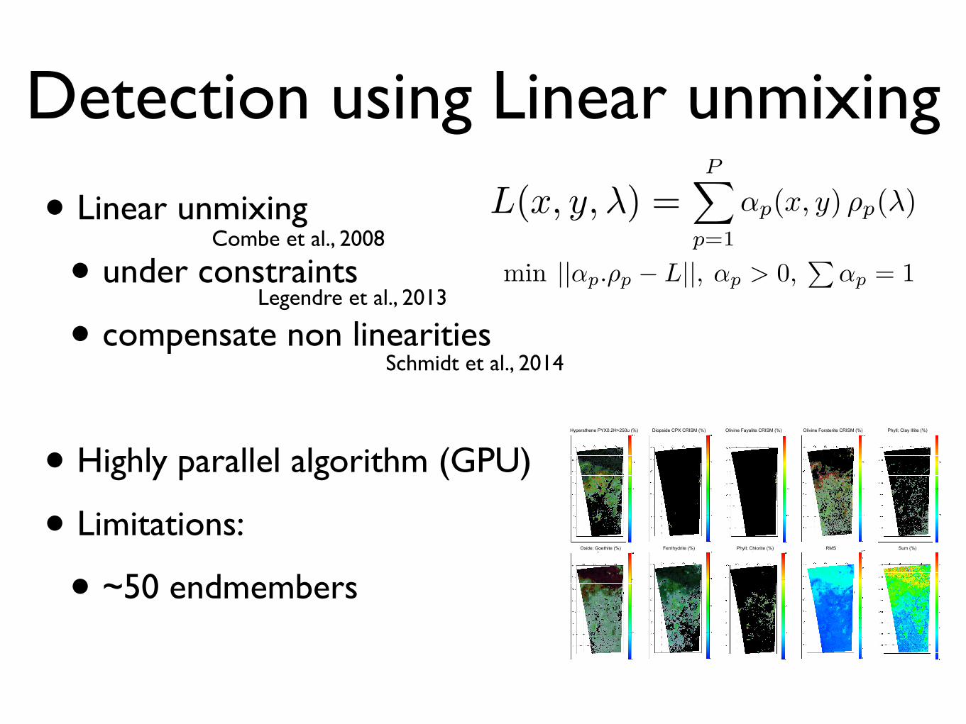
Detection using Linear unmixing

• Linear unmixing

• under constraints

• compensate non linearities

• Highly parallel algorithm (GPU)

• Limitations:

• ~50 endmembers

Legendre et al., 2013

Acc

epte

d man

uscrip

t

ponents (ICs), we have to pay attention to their physicalinterpretation. In fact, additional knowledges can be used.In this purpose: (i) synthetic reference spectra of the mainendmembers obtained after inversion [4]; (ii) a supervisedclassification using wavalet transform called wavangletwhich is in accordance with Mars physical knowledge [5].Finally, a last di!culty is to check the relevance of thelinear mixture model as well as the hypothesis on whichthe algorithm is based.

From a methodological point of view, the objective ofthis paper is to point out that, when source independenceassumption is not fully satisfied, an ICA algorithm can pro-vide spurious ICs and one has to prefer semi-blind meth-ods which relax partially independence assumption and ac-counts for additional informations. Especially, in hyper-spectral imaging an evident prior concerns the positivity ofthe images and the component spectra.

The paper is organized as follows. Section 2 presents thesimplified observation model in the case of a geographi-cal mixture and the possible decomposition models. Sec-tion 3 recalls briefly the source separation problem. Section4 presents the results when applying ICA to hyperspec-tral data, and discuss the relevance of the separation. Sec-tion 5 introduces the Bayesian framework and shows howBayesian methods can ensure the positivity of the sourcesand of the mixing coe!cients. The results on Mars hyper-spectral data are then discussed. Section 7 recalls the mainresults and gives some perspectives of this research work.

2. Hyperspectral Data Modeling

The OMEGA spectrometer, carried by Mars Expressspacecraft on an elliptical orbit, has a spatial resolutionrange from 300 m to 4 km. This instrument has three chan-nels, a visible channel and two near infrared channels. Wewill focus in this work only on the near infrared channelssince the behavior between major chemicals can be dis-criminated in this spectral range. The analysis is focusedon a data set consisting in a single hyperspectral data cubeobtained by looking to the South Polar Cap of Mars inthe local summer where CO2 ice, water ice and dust werepreviously detected [5, 6]. This data cube is made up with2 channels: 128 spectral planes from 0.93 µm to 2.73 µmwith a resolution of 0.013µm and 128 spectral planes from2.55µm to 5.11µm with a resolution of 0.020µm. After cal-ibration, the dimensionless physical unit used to expressthe spectra is the ”reflectance”, which is the ratio betweenthe irradiance leaving each pixel toward the sensor and thesolar irradiance at the ground. Interactions between pho-tons coming from the sun and the planet Mars, through itsatmosphere and surface, allows us to identify the di"erentcompounds present in the planet. Those compounds aremixed and usually di"erent chemical species can be identi-fied in each measured spectra. Two kinds of physical mixingat the ground can be observed [7]:– Geographic mixture: each pixel is a patchy area made

of several pure compounds. This type of mixture, some-times called ”sub-pixel mixture”, happens when the spa-tial resolution is not large enough to observe the complexgeological combination pattern. The total reflectance inthis case will be a weighted sum of the pure constituentreflectances. The weights (abundance fractions) associ-ated to each pure constituent are surface proportions in-side the pixel.

– Intimate mixture: each pixel is made of one single terraintype which is a mixture at less than the typical mean-path scale (typically the order of 1mm scale). The totalreflectance in this case will be a nonlinear function ofpure constituent reflectances.

The case of intimate mixtures, which needs nonlinear sourceseparation methods and further development, is not ad-dressed here. In this paper, we perform our analysis withhypothesis of a geographical mixtures and hence linear mix-ing models.

2.1. Observation Model

The hyperspectral images can be modeled by examiningall the factors that contribute to the radiance signal reach-ing the sensor after interaction of the sunlight with a plan-etary surface. An analytical expression of the measured ra-diance factor in a case of a Lambertian surface 2 with ahomogeneous atmosphere has been proposed in [8], underthe following assumptions: (i) the multiple di"usion termr and the di"usion terms E(µ) are negligible, (ii) the paththrough the atmosphere is equivalent for all pixels, (iii) thedirect atmospheric contribution only depends on the wave-length, (iv) the emergence direction is always the same.Thus, based on this model and using the geographic mix-ture assumption, the radiance factor at location (x, y) andat wavelenght ! satisfies the following observation model:

L(x, y, !) =!

"a(!) + #(!)P"

p=1

#p(x, y) "p(!)

#cos [$(x, y)] (1)

where #(!) is the spectral atmospheric transmission,$(x, y) the angle between the solar direction and the sur-face normal (solar incidence angle), P the number ofendmembers in the region of coordinates (x, y), "p(!) thespectrum of the p-th endmember, #p(x, y) its weight inthe mixture and "a(!) the radiation that did not arrivedirectly from the area under view. This mixture model canalso be written as:

L(x, y, !) =P"

p=1

#!p(x, y) · "!p(!) + E(x, y, !) (2)

where

2 a surface that reflects the light independently of both incidenceand emergence directions

2

Acc

epte

d man

uscrip

t

ponents (ICs), we have to pay attention to their physicalinterpretation. In fact, additional knowledges can be used.In this purpose: (i) synthetic reference spectra of the mainendmembers obtained after inversion [4]; (ii) a supervisedclassification using wavalet transform called wavangletwhich is in accordance with Mars physical knowledge [5].Finally, a last di!culty is to check the relevance of thelinear mixture model as well as the hypothesis on whichthe algorithm is based.

From a methodological point of view, the objective ofthis paper is to point out that, when source independenceassumption is not fully satisfied, an ICA algorithm can pro-vide spurious ICs and one has to prefer semi-blind meth-ods which relax partially independence assumption and ac-counts for additional informations. Especially, in hyper-spectral imaging an evident prior concerns the positivity ofthe images and the component spectra.

The paper is organized as follows. Section 2 presents thesimplified observation model in the case of a geographi-cal mixture and the possible decomposition models. Sec-tion 3 recalls briefly the source separation problem. Section4 presents the results when applying ICA to hyperspec-tral data, and discuss the relevance of the separation. Sec-tion 5 introduces the Bayesian framework and shows howBayesian methods can ensure the positivity of the sourcesand of the mixing coe!cients. The results on Mars hyper-spectral data are then discussed. Section 7 recalls the mainresults and gives some perspectives of this research work.

2. Hyperspectral Data Modeling

The OMEGA spectrometer, carried by Mars Expressspacecraft on an elliptical orbit, has a spatial resolutionrange from 300 m to 4 km. This instrument has three chan-nels, a visible channel and two near infrared channels. Wewill focus in this work only on the near infrared channelssince the behavior between major chemicals can be dis-criminated in this spectral range. The analysis is focusedon a data set consisting in a single hyperspectral data cubeobtained by looking to the South Polar Cap of Mars inthe local summer where CO2 ice, water ice and dust werepreviously detected [5, 6]. This data cube is made up with2 channels: 128 spectral planes from 0.93 µm to 2.73 µmwith a resolution of 0.013µm and 128 spectral planes from2.55µm to 5.11µm with a resolution of 0.020µm. After cal-ibration, the dimensionless physical unit used to expressthe spectra is the ”reflectance”, which is the ratio betweenthe irradiance leaving each pixel toward the sensor and thesolar irradiance at the ground. Interactions between pho-tons coming from the sun and the planet Mars, through itsatmosphere and surface, allows us to identify the di"erentcompounds present in the planet. Those compounds aremixed and usually di"erent chemical species can be identi-fied in each measured spectra. Two kinds of physical mixingat the ground can be observed [7]:– Geographic mixture: each pixel is a patchy area made

of several pure compounds. This type of mixture, some-times called ”sub-pixel mixture”, happens when the spa-tial resolution is not large enough to observe the complexgeological combination pattern. The total reflectance inthis case will be a weighted sum of the pure constituentreflectances. The weights (abundance fractions) associ-ated to each pure constituent are surface proportions in-side the pixel.

– Intimate mixture: each pixel is made of one single terraintype which is a mixture at less than the typical mean-path scale (typically the order of 1mm scale). The totalreflectance in this case will be a nonlinear function ofpure constituent reflectances.

The case of intimate mixtures, which needs nonlinear sourceseparation methods and further development, is not ad-dressed here. In this paper, we perform our analysis withhypothesis of a geographical mixtures and hence linear mix-ing models.

2.1. Observation Model

The hyperspectral images can be modeled by examiningall the factors that contribute to the radiance signal reach-ing the sensor after interaction of the sunlight with a plan-etary surface. An analytical expression of the measured ra-diance factor in a case of a Lambertian surface 2 with ahomogeneous atmosphere has been proposed in [8], underthe following assumptions: (i) the multiple di"usion termr and the di"usion terms E(µ) are negligible, (ii) the paththrough the atmosphere is equivalent for all pixels, (iii) thedirect atmospheric contribution only depends on the wave-length, (iv) the emergence direction is always the same.Thus, based on this model and using the geographic mix-ture assumption, the radiance factor at location (x, y) andat wavelenght ! satisfies the following observation model:

L(x, y, !) =!

"a(!) + #(!)P"

p=1

#p(x, y) "p(!)

#cos [$(x, y)] (1)

where #(!) is the spectral atmospheric transmission,$(x, y) the angle between the solar direction and the sur-face normal (solar incidence angle), P the number ofendmembers in the region of coordinates (x, y), "p(!) thespectrum of the p-th endmember, #p(x, y) its weight inthe mixture and "a(!) the radiation that did not arrivedirectly from the area under view. This mixture model canalso be written as:

L(x, y, !) =P"

p=1

#!p(x, y) · "!p(!) + E(x, y, !) (2)

where

2 a surface that reflects the light independently of both incidenceand emergence directions

2

min ||αp.ρp − L||min ||αp.ρp − L||, αp > 0,

�αp = 1

1

Combe et al., 2008

Schmidt et al., 2014

Olivine Fayalite CRISM (%)Hypersthene PYX0.2H>250u (%) Olivine Forsterite CRISM (%)Diopside CPX CRISM (%) Phyll; Clay Illite (%)

Sum (%)

OMEGA ORB422_4

RMSPhyll; Chlorite (%)Ferrihydrite (%)Oxide; Goethite (%)

Figure 8: Detection of 8 minerals over 44 spectra on OMEGA image ORB422_4 of Syrtis

Major using IPLS in the hue-saturation-value color system. The hue (color) represents the

mixing coefficient. The saturation (color or b/w) represents the error. The value (intensity of

color or b/w) represents the rms. Spectral mixing coefficient map are shown with following

conditions : (i) maximum mixing coefficient > 5% , (ii) error on mixing coefficient < mixing

coefficient, and (iii) RMS < 10x the dark current noise (see text). Pyroxene, olivines, phyl-

losilicates, ferrihydrite and oxides are detected and the corresponding “mixing coefficient“ are

mapped (color refer to the online version of the article).

14

• Detection


•Quantification



Grain size Free mean path

Spectral shape = physical state

100 µm

10 mm

Douté, et al, JGR, 1998 Schmitt, et al, Solar System Ice, 1998

Quantitative compositional analysis of martian mafic regions 75

Fig. 5. Sensitivity to the grain size. (A) The OMEGA spectrum (black line) is com-pared to three models. The best fit (red line) is obtained by assuming all theparameters free (see Table 2 for final results) and was already shown in Fig. 3. Ifthe grain size is forced to be 100 (blue spectrum) or 200 µm (green spectrum), thefits are slightly degraded. (B) The abundances of three major minerals correspondto the simulations shown in (A).

between measured spectrum and computed spectrum (Press et al.,2002). This optimization procedure depends on the initial condi-tions. We design another sensitivity test to discuss the effect of theinput parameters on the validity of the inferred modal mineralogy.We vary the starting grain size and abundance parameters for eachend-member and assess the consistency of resultant grain size andabundance solutions. The test is done on a large number of spectraextracted from the DCT unit of Terra Meridiani in order to betterevaluate the uncertainties. Comparison between the two simula-tions shows that the final average values of the abundances varyonly slightly with the values of the starting parameters (Fig. 7):28± 3% versus 28 ± 5% for HCP, 10± 4% versus 12± 3% for LCPand 52± 4% versus 47 ± 7% for plagioclase. Of special interest isthe increase of pyroxene abundances versus the pyroxene banddepth value. This expected compositional trend makes us confi-dent on the methodology and the values of the abundances. Theplagioclase abundance is less robust but the distributions and theaveraged values of abundances are still consistent within the un-certainties of the method (!10%). By contrast, the initial conditionssignificantly affect the grain size parameter. As the input grain sizeparameter decreases or increases, the resultant solutions similarlyshifted to the same part of the parameter space. For instance, thefinal grain sizes of HCP are close to the initial value of 100 µm forsimulation 1, while the grain sizes of the simulation 2 that startedwith a 300 µm value, are ranged between 200 and 500 µm. Thisreveals that the starting parameters do have a significant effect on

Fig. 6. Effect of the grain size of plagioclase. (A) Data spectrum compared to fourmodel-derived spectra for which the size of plagioclase grains is fixed to 10 µm (redspectrum), 100 µm (orange), 500 (cyan), and 1000 µm (green). The blue spectrumindicates the best fit when all the parameters including the plagioclase grain sizeare free. In this case, the grain size of plagioclase is a free parameter. (B) Abundanceof the different minerals for the five fitting procedures shown in (A). RMS is con-sidered to be acceptable when it is smaller than 0.30%. (For interpretation of thereferences to color in this figure legend, the reader is referred to the web version ofthis article.)

the resultant solutions whatever the mineral. However, the rangesof the final acceptable solutions can be evaluated. Most of the finalvalues of the plagioclase grain size clearly plot in the 50–150 µmrange for the two simulations. The same trend is observed for theLCP component. The HCP grain size shows large standard deviation,but still in the range of a few 10s to a few 100s of micrometers asdiscussed previously.

The simplex algorithm calculates thousands of possible mix-tures before reaching a final solution. In order to illustrate therange of values considered in the fitting effort and provide anestimate of the uncertainty in the final results, we plot the RMSversus component abundances and diameters for several represen-tative pyroxene band depths (0.01, 0.02, 0.03, 0.04, 0.05 and 0.06)in Fig. 8. Apart from the grain size of the martian dust compo-nent that is initially fixed, the grain sizes are ranged in the 10sto a few 100s µm, which confirms the previous estimates. The pa-rameter space of the abundances is 40–55% for plagioclase, 25–35%for HCP, 10–15% for LCP, 5–10% for the dust, and less than 5–10%for olivine. These variations are also in good agreement with theuncertainties previously determined. For a given spectrum and forvalues of RMS lower than 0.35%, the excursions of the parameterare even smaller.

3.4. Sensitivity to the olivine mineral

Olivine has strong absorption bands in the wavelength rangeunder consideration, and its abundance should be well constrained.

• Minimisation technique

• Surface

• Atmosphere

• Limitations

• Slow

• Multiples solutions

Inversion using Least square

Poulet et al., 2009

Wolff et al., 2009

similar showing that the area of interest does not contain asmuch dust as the wavanglet methodology predicts. On thecontrary, estimations given by GRSIR are more coherentwith this spectral analysis.

6.3. Discussion of the Southern Permanent CapProperties

[47] The parameter maps estimated by GRSIR are geore-ferenced using ancillary data provided by the OMEGA teamand then are merged into global geographical mosaics. Thelatter covers the entire bright permanent polar cap (BPPC)with the exception of a limited area centered around(89!270S, 34!580W). We focus on the absolute variationsof four unconstrained parameters: water ice and dust pro-

portions, water and CO2 ice grain size (Figure 10). Themosaics do show very few artificial discontinuities acrossthe cap contrary to counterparts that we generated usingparameter maps obtained by k-NN. This smoothness is anadditional proof that GRSIR gives consistent results fromobservations acquired by OMEGA under different condi-tions. The different parameters do not show any obviousintercorrelation. Furthermore the mosaics provide a picturethat is comptatible in its broad lines with the one drawn byDoute et al. [2007a]. These authors estimated trends ofvariations for water and dust contents in the CO2 ice of theBPPC by combining classification techniques and selectivephysical modeling of individual representative spectra (seesection 3.3 and Figure 13 of the latter paper). Mosaics of

Figure 10. Global mosaics illustrating the absolute variations of (a) water ice and (b) dust proportions,as well as (c) water ice and (d) CO2 ice grain sizes across the entire permanent bright polar cap. They arederived from individual parameter maps obtained by inversing OMEGA observations 41, 61, and 103with GRSIR.

E06005 BERNARD-MICHEL ET AL.: RETRIEVAL OF MARS SURFACE PROPERTIES

12 of 14

E06005

Inversion using Linear Subspace• Look up table

• GRSIR

• Projection into a linear subspace

• Very fast

• Limitations:

• Non linearities

• Multiple solutions

Bernard-Michel et al., Statistic and computing, 2009Bernard-Michel et al., JGR, 2009

Douté et al., LPSC, 2007

CO2 ice grain size

Bayesian Inversion

!• Maximum likelihood inversion

Andrieu, F. et al., in preparation

• Monte Carlo inversion on photometry

• Limitations:

• Computation time

Ceamanos et al., 2013Fernando, J. et al., 2013

Data Science Challenges for hyperspectral images

• Radiative transfer inversion (bayesian technique)

• estimation of surface/atmospheric properties

• How to represent the data (global map, wavelength, time) ?

Conclusion

• Planetary Science (and Geoscience) needs Data Science revolution

• Data Mining

• Data visualisation

• Massive data treatment

• Virtual Observatory

Data Science for Planetary Science - indico.lal.in2p3.fr fileData Science for Planetary Science...

Documents

Transcript of Data Science for Planetary Science - indico.lal.in2p3.fr fileData Science for Planetary Science...