Proc. IODP | Volume 320/321

Chapter contents

Abstract . . . . . . . . . . . . . . . . . . . . . . . . . . . . . . . 1

Introduction . . . . . . . . . . . . . . . . . . . . . . . . . . . 1

X-ray fluorescence analytical technique . . . . . . 2

Data acquisition methods . . . . . . . . . . . . . . . . . 2

Data reduction methods for later calibration: normalized median-scaled method . . . . . . . . 3

Example calibration of data: BaSO4 . . . . . . . . . 5

Results and discussion . . . . . . . . . . . . . . . . . . . . 5

Conclusions . . . . . . . . . . . . . . . . . . . . . . . . . . . . 6

Acknowledgments. . . . . . . . . . . . . . . . . . . . . . . 6

References . . . . . . . . . . . . . . . . . . . . . . . . . . . . . 6

Figures . . . . . . . . . . . . . . . . . . . . . . . . . . . . . . . . 8

Tables. . . . . . . . . . . . . . . . . . . . . . . . . . . . . . . . 161Lyle, M., Olivarez Lyle, A., Gorgas, T., Holbourn, A., Westerhold, T., Hathorne, E., Kimoto, K., and Yamamoto, S., 2012. Data report: raw and normalized elemental data along the Site U1338 splice from X-ray fluorescence scanning. In Pälike, H., Lyle, M., Nishi, H., Raffi, I., Gamage, K., Klaus, A., and the Expedition 320/321 Scientists, Proc. IODP, 320/321: Tokyo (Integrated Ocean Drilling Program Management International, Inc.). doi:10.2204/iodp.proc.320321.203.20122Department of Oceanography, Texas A&M University, College Station TX 77843, USA. Correspondence author: mlyle@ocean.tamu.edu3Integrated Ocean Drilling Program, Texas A&M University, 1000 Discovery Drive, College Station TX 77845-9547, USA.4Institut für Geowissenschaften, Christian-Albrechts-Universität zu Kiel, Olhausenstrasse 40, 24098 Kiel, Germany.5Center for Marine Environmental Sciences (MARUM), University of Bremen, PO Box 330440, 28334 Bremen, Germany.6IFM-GEOMAR, Leibniz Institute of Marine Sciences at University of Kiel, Wischhofstrasse 1-3, D-24148 Kiel, Germany.7Institute of Observational Research for Global Change (IORGC), Japan Agency for Marine-Earth Science and Technology, 2-15 Natsushima-Cho, Yokosuka 237-0061, Japan.8Institute of Low Temperature Science, Hokkaido University, N19W8, Kita-Ku, Sapporo 060-0819, Japan.

Data report: raw and normalized elementaldata along the Site U1338 splice from X-ray

fluorescence scanning1

Mitchell Lyle,2 Annette Olivarez Lyle, Thomas Gorgas,3 Ann Holbourn,4 Thomas Westerhold,5

Ed Hathorne,6 Katsunori Kimoto,7 and Shinya Yamamoto8

Pälike, H., Lyle, M., Nishi, H., Raffi, I., Gamage, K., Klaus, A., and the Expedition 320/321 ScientistsProceedings of the Integrated Ocean Drilling Program, Volume 320/321

AbstractWe used X-ray fluorescence (XRF) scanning on Site U1338 sedi-ments from Integrated Ocean Drilling Program Expedition 321 tomeasure sediment geochemical compositions at 2.5 cm resolutionfor the 450 m of the Site U1338 spliced sediment column. Thisspatial resolution is equivalent to ~2 k.y. age sampling in the 0–5Ma section and ~1 k.y. resolution from 5 to 17 Ma. Here we reportthe data and describe data acquisition conditions to measure Al,Si, K, Ca, Ti, Fe, Mn, and Ba in the solid phase. We also describe amethod to convert the data from volume-based raw XRF scandata to a normalized mass measurement ready for calibration byother geochemical methods. Both the raw and normalized dataare reported along the Site U1338 splice.

IntroductionA primary objective of the Integrated Ocean Drilling Program(IODP) Pacific Equatorial Age Transect (PEAT) project is to pro-duce continuous records that track the effects of climate changein the equatorial Pacific with enough detail to resolve orbitallyforced climate cycles. A significant part of climate change is re-corded by variability in the chemical composition of sediments,but this information typically is hard to extract at a reasonablecost.

X-ray fluorescence (XRF) scanning is potentially an economicalway to extract the chemical data—it is an X-ray optical techniquethat can measure most major elements and some minor ones in~20–30 s per measurement. This method can be used to gatherchemical data at vertical spacing similar to that at which physicalproperties data are gathered (e.g., Westerhold and Röhl, 2009).These chemical measurements can augment physical propertiesmeasurements to study cyclostratigraphy, and if calibrated, XRFscan data can be used to understand the long-term evolution ofbiogeochemical cycles.

In this data report, we present the results of XRF scanning on thespliced sedimentary section of PEAT Site U1338 and describe a ba-sic technique to normalize and calibrate the data for further geo-chemical study. Both the raw and normalized data along thesplice are presented in tables. Data at this sampling resolution forthe first time allows the study of geochemical cycles for long peri-ods in the Miocene and of how biogeochemical changes are

doi:10.2204/iodp.proc.320321.203.2012

M. Lyle et al. Data report: elemental data by XRF

associated with long-term changes in global cli-mate.

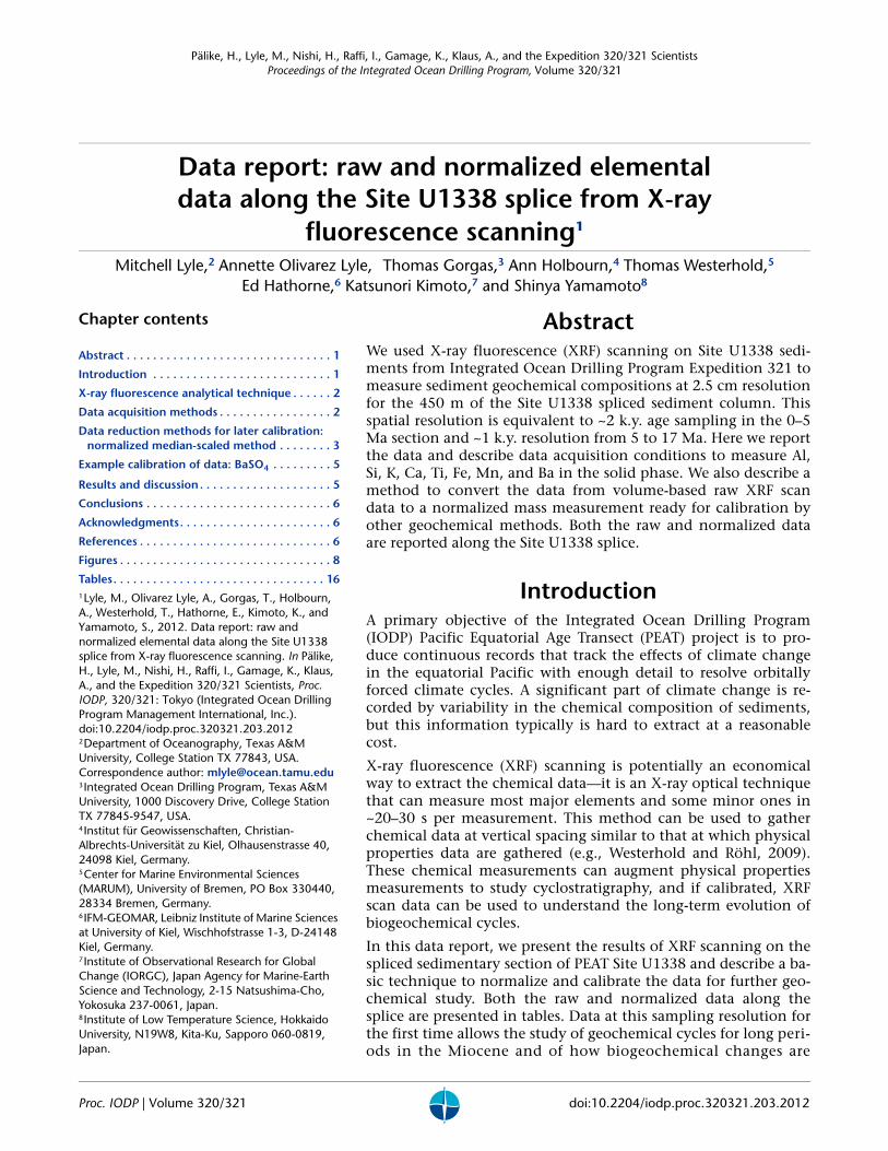
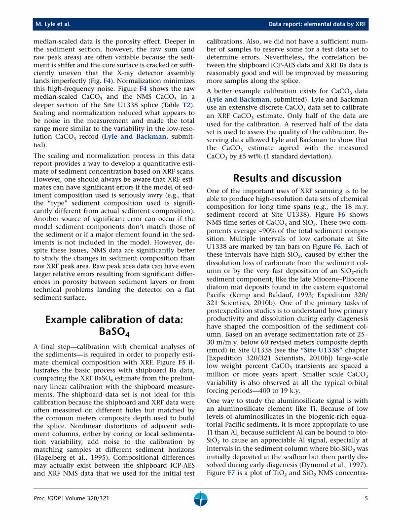
Site U1338 (Fig. F1; 2°30.469′N, 117°58.178′W; 4200 mwater depth) is on 18 Ma ocean crust buried by ~400m of pelagic sediment (see the “Site U1338” chapter[Expedition 320/321 Scientists, 2010b]). The sedi-ment drapes over topography so that the ~200 mabyssal hill relief on basement is still visible despitethe 400 m of sediment cover (Tominaga et al., 2011).

Site U1338 has the characteristic variations in sedi-mentary calcium carbonate content that result in thecommon seismic stratigraphy that is found through-out the equatorial Pacific region east of Hawaii(Mayer et al., 1985, 1986; see the “Site U1338” chap-ter [Expedition 320/321 Scientists, 2010b]; Tominagaet al., 2011). It has been a long-standing scientificproblem to understand what forcing mechanismsand associated variations in global geochemical cy-cles caused the carbonate cycles that in turn causedthe common seismic horizons across the equatorialPacific. XRF scanning potentially can determine cal-cite contents with sufficient detail to better under-stand both the links between physical properties andsediment carbonate contents and why sedimentarycarbonate varied throughout the eastern equatorialPacific.

XRF studies of biogeochemically active elements Ca,Si, and Ba also can be used to understand changes inproductivity and can be compared to changes inpreservation to better understand changes in the car-bon cycle. XRF scanning also can measure alumino-silicate elements (Al, K, and Ti) to understand dustdeposition in the equatorial Pacific, whereas mea-surements of the redox-sensitive elements Fe andMn can be used to study changes in the sedimentaryredox environment and hydrothermal activity. Dy-mond (1981) shows how chemical data can be usedto discern sediment processes in the eastern equato-rial Pacific.

X-ray fluorescenceanalytical technique

X-ray fluorescence is an analytical technique thatuses the characteristic fluorescence of elements ex-posed to high-energy X-ray illumination as a meansto estimate a sample’s chemical composition. High-energy X-ray photons eject inner-shell electronsfrom atoms being illuminated by the X-rays (Jansenet al., 1998). Outer shell electrons in higher energylevels then occupy these lower energy levels, releas-ing the excess energy as characteristic XRF for eachelement. The intensity of the fluorescence from a

Proc. IODP | Volume 320/321

sample can be used to determine the abundance ofdifferent elements.

XRF is a volume and not a mass measurement, how-ever. A conventional chemical analysis measures theamount of an element in a standard mass of totalmaterial; a sample with 8 wt% Fe has, for example,8 g Fe per 100 g sample. For XRF, in contrast, the X-ray source illuminates a certain volume of sediment,and the amount of X-rays returned in part dependson the mass of sediment in that volume. Low atomicweight elements emit lower energy X-rays than highatomic weight elements, and these low-energy X-rays are more easily absorbed by other elements asthey pass out of the sample. For this reason, light el-ements have a smaller characteristic emission vol-ume than heavy elements (Tjallingii et al., 2007),causing problems if the sample is not homogeneous.

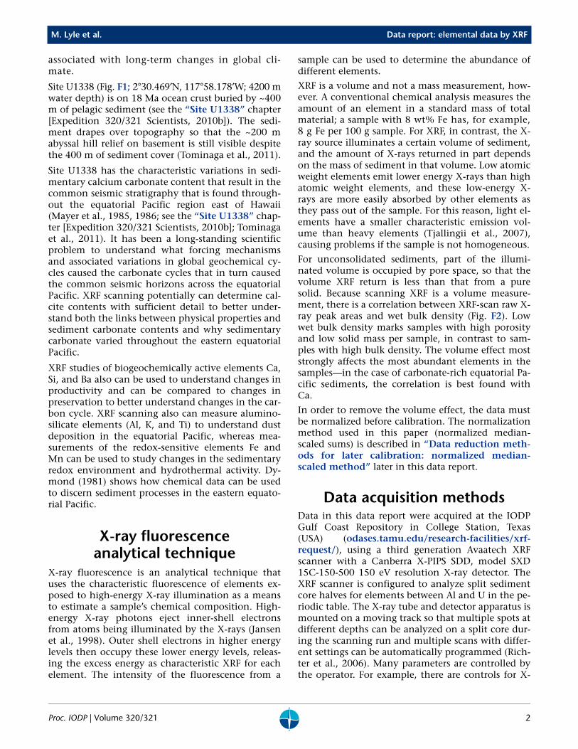
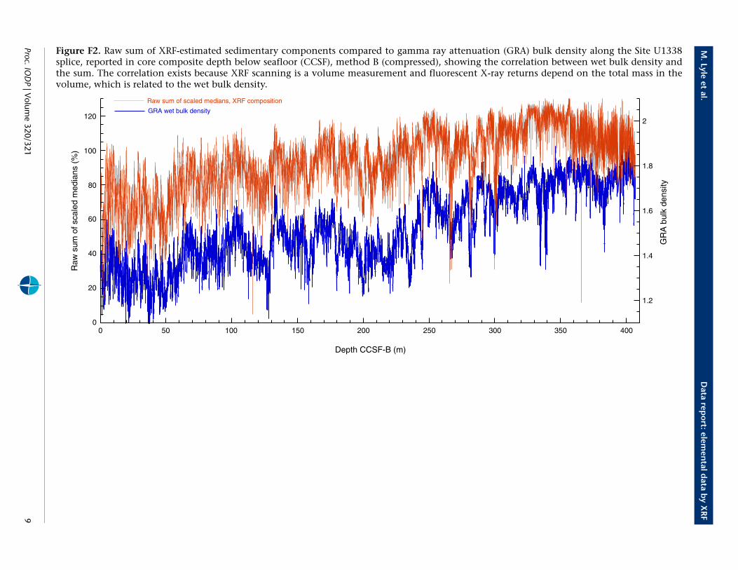
For unconsolidated sediments, part of the illumi-nated volume is occupied by pore space, so that thevolume XRF return is less than that from a puresolid. Because scanning XRF is a volume measure-ment, there is a correlation between XRF-scan raw X-ray peak areas and wet bulk density (Fig. F2). Lowwet bulk density marks samples with high porosityand low solid mass per sample, in contrast to sam-ples with high bulk density. The volume effect moststrongly affects the most abundant elements in thesamples—in the case of carbonate-rich equatorial Pa-cific sediments, the correlation is best found withCa.

In order to remove the volume effect, the data mustbe normalized before calibration. The normalizationmethod used in this paper (normalized median-scaled sums) is described in “Data reduction meth-ods for later calibration: normalized median-scaled method” later in this data report.

Data acquisition methodsData in this data report were acquired at the IODPGulf Coast Repository in College Station, Texas(USA) (odases.tamu.edu/research-facilities/xrf-request/), using a third generation Avaatech XRFscanner with a Canberra X-PIPS SDD, model SXD15C-150-500 150 eV resolution X-ray detector. TheXRF scanner is configured to analyze split sedimentcore halves for elements between Al and U in the pe-riodic table. The X-ray tube and detector apparatus ismounted on a moving track so that multiple spots atdifferent depths can be analyzed on a split core dur-ing the scanning run and multiple scans with differ-ent settings can be automatically programmed (Rich-ter et al., 2006). Many parameters are controlled bythe operator. For example, there are controls for X-

2

M. Lyle et al. Data report: elemental data by XRF

ray tube current, voltage, measurement time (livetime), X-ray filters used, and area of X-ray illumina-tion. The downcore position step is precise to 0.1 mm.

For Site U1338 XRF scans, sample spacing along eachcore section was set at 2.5 cm intervals and separatescans at two voltages were used. One scan was per-formed at 10 kV for the elements Al, Si, S, Cl, K, Ca,Ti, Mn, and Fe, and a repeat scan was performed at50 kV for Ba. The voltage used for elements mea-sured is determined by the energy needed to excitethe appropriate characteristic X-rays. The X-ray illu-mination area was set at 1.0 cm in the downcore di-rection and 1.2 cm in the cross-core direction, andthe scan was run down the center of the split corehalf (6.8 cm total diameter). Both scans were donewith an X-ray tube current of 2 mA. Settings used forSite U1338 10 kV XRF scans are 2 mA tube current,no filter, and a detector live time of 20 s; for the 50kV scan the settings are 2 mA current, Cu filter, and adetector live time of 10 s.

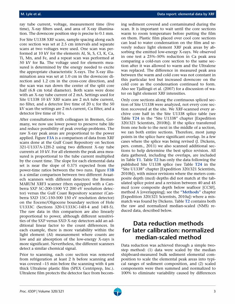
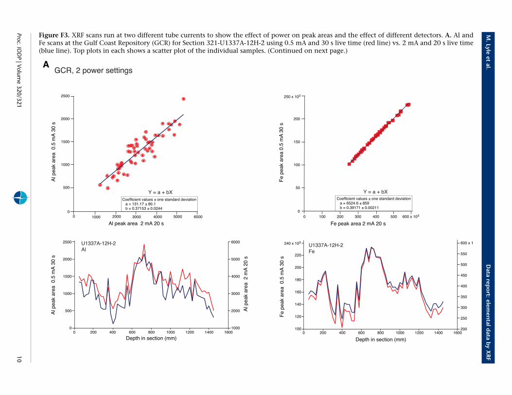
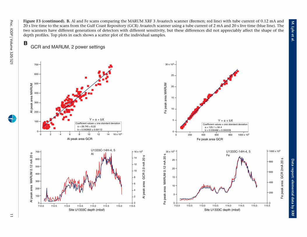
After consultations with colleagues in Bremen, Ger-many, we now use lower power to preserve tube lifeand reduce possibility of peak overlap problems. Theraw X-ray peak areas are proportional to the powerapplied. Figure F3A is a comparison of data from XRFscans done at the Gulf Coast Repository on Section321-U1337A-12H-2 using two different X-ray tubecurrents at 10 kV. For all elements the peak area mea-sured is proportional to the tube current multipliedby the count time. The slope for each elemental dataset is near the slope of 0.375 expected from thepower-time ratios between the two runs. Figure F3Bis a similar comparison between two different Avaat-ech scanners with different detectors: the BremenMARUM XRF3 scanner (then equipped with a Can-berra SXP 5C-200-1500 V2 200 eV resolution detec-tor) versus the Gulf Coast Repository scanner (Can-berra SXD 15C-150-500 150 eV resolution detector)on the Eocene/Oligocene boundary section of HoleU1333C (Sections 320-U1333C-14H-4 and 14H-5).The raw data in this comparison are also linearlyproportional to power, although different sensitivi-ties of the SXP versus SXD X-ray detectors add an ad-ditional linear factor to the count differences. Ineach example, there is more variability within thelight element (Al) measurement where counts arelow and air absorption of the low-energy X-rays ismore significant. Nevertheless, the different scannersdetect a similar chemical signal.

Prior to scanning, each core section was removedfrom refrigeration at least 2 h before scanning andwas covered ~15 min before the scanning with 4 µmthick Ultralene plastic film (SPEX Centriprep, Inc.).Ultralene film protects the detector face from becom-

Proc. IODP | Volume 320/321

ing sediment covered and contaminated during thescan. It is important to wait until the core sectionswarm to room temperature before putting the filmon them. Plastic film placed over cool core sectionscan lead to water condensation on the film and se-verely reduce light element XRF peak areas by ab-sorbing the emitted low-energy X-rays. We observedin one test a 25%–50% reduction in Ca peak areacomparing a cold-run core section to the same sec-tion after it was allowed to warm and the Ultralenewas replaced. The difference in measured peak areabetween the warm and cold core was not constant inthis particular test but increased downcore on thecold core as the condensation continued to form.Also see Tjallingii et al. (2007) for a discussion of wa-ter on light element XRF intensities.

Only core sections along the continuous spliced sec-tion of Site U1338 were analyzed, not every core sec-tion recovered at the site. We XRF-scanned every ar-chive core half in the Site U1338 splice table (seeTable T24 in the “Site U1338” chapter [Expedition320/321 Scientists, 2010b]). If the splice transferredfrom one hole to the next in the middle of a section,we ran both entire sections. Therefore, most jumppoints in the splice have significant overlap. In a fewcases where the splice was being revised (J. Dickens,pers. comm., 2011) we also scanned additional sec-tions to help determine the best splice revision. Alldata gathered, including the overlaps, are includedin Table T1. Table T2 has only the data following thepublished Site U1338 splice (see Table T24 in the“Site U1338” chapter [Expedition 320/321 Scientists,2010b]), with minor revisions where the meters com-posite depth (mcd) depths did not match at the tab-ulated splice point and a revision between 40 and 45mcd (core composite depth below seafloor [CCSF],method A [overlapping]; see the “Methods” chapter[Expedition 320/321 Scientists, 2010a]) where a mis-match was found by Dickens. Table T2 contains boththe raw and normalized median-scaled (NMS) re-duced data, described below.

Data reduction methods for later calibration: normalized

median-scaled methodData reduction was achieved through a simple two-step method: (1) data were scaled by the medianshipboard-measured bulk sediment elemental com-position to scale the elemental peak areas into typi-cal ranges of sediment composition, and (2) scaledcomponents were then summed and normalized to100% to eliminate variability caused by differences

3

M. Lyle et al. Data report: elemental data by XRF

in porosity or cracks. This method of data reductionhas a few similarities and several differences withthat of Weltje and Tjallingii (2008). Weltje andTjallingii (2008) normalize the peak areas first andthen log transform the peak areas to reduce therange between major and minor XRF-emitters, likeour median-scaling step. Finally, they solve a matrixof XRF element/element ratios for composition. TheWeltje and Tjallingii (2008) approach has the advan-tage of being more global and developed from firstprinciples, but it suffers from complexity and is noteasily adapted. The advantage of the NMS techniqueis that it can be quickly implemented, and the cali-bration step can be used to determine if a more de-tailed approach is needed.

Sample scalingSample scaling is needed to better match the rangeof XRF peak area measurements to the range ofchemical composition along the scan. Without scal-ing, normalized peak areas can be dominated by ef-fects of one element.

For an elemental scaling Se,

Se = Med%e × (PeakAreae/PeakAreae,med),

where Med%e is the median weight percent of a sedi-mentary component (e.g., for Fe, we used the oxideFe2O3, and for Ca, CaCO3). PeakAreae is the measuredelemental peak area in a sample, and PeakAreae,med isthe median peak area over the data set. There may beerrors in absolute scaling because the chemicalanalyses are far fewer than the XRF sampling. Theraw CaCO3 data, for example, scales from 0% to~120%. However, the normalizing step reduces thetotal range to between 0% and 100%, and the cali-bration step correlating the scaled data to ground-truth chemical analyses produces a linear correlationthat does a final adjustment to the percentage data.

Scaling the raw peak areas was done because the pro-duction of characteristic X-rays of different elementsdoes not scale linearly with elemental ratios in thesample. Scaling to the total summed peak area wasrejected because scaling to raw peak area stronglyoverweights Ca in the carbonate-rich sediment col-umn of Site U1338 and is a significant cause of non-linearities in later calibration. Scaling to total peakarea is effectively equivalent to scaling to Ca peakarea, as is shown by comparing Ca proportions inthe two scaling schemes. Median peak area of Ca is95% of summed total median peak area, whereas me-dian CaCO3 is 76% of the summed shipboard chemi-cal analyses. The raw peak area Ca/Si ratio is 38.5,whereas the ratio of median CaCO3/SiO2 from ship-

Proc. IODP | Volume 320/321

board inductively coupled plasma–atomic emissionspectroscopy (ICP-AES) analyses is 4.9. Summing toraw peak areas thus creates a burden that must be re-moved by the calibration step, whereas scaling tomedian values reduces the problem.

We scaled each element independently to a medianof the compositional data from shipboard ICP-AESanalyses (see the “Site U1338” chapter [Expedition320/321 Scientists, 2010b]). Although the shipboardcompositional data set is a much smaller sample setthan the XRF scan data, it is appropriate for scalingas long as the compositional data set is a reasonablerepresentation of the total range of composition. Thescaling step could also be done with a generic aver-age for the sediment type being studied if chemicaldata were not available. The use of a different “type”compositional analysis to scale the median value willchange the ultimate NMS value and will then poten-tially change the slope of the calibration line to con-vert from NMS to calibrated percent. It is thus impor-tant to use the same scaling values within a commoncalibration.

Normalizing sample composition to 100%Ideally, the sum of all sediment components shouldbe 100% if all major elements are measured and theyare properly converted to the appropriate sedimen-tary components (e.g., Ca is represented in the sedi-ment by the sedimentary component CaCO3, notCaO). However, The XRF-scaled sum of componentsis often much lower than 100% near the top of thesection where porosity is high and dry sample massin the scan area is low. We used the following com-ponents for our data set: Al2O3, SiO2, K2O, CaCO3,TiO2, MnO, Fe2O3, and BaSO4. From the shipboardchemical analyses, these components sum to a me-dian of 94.7 wt% and adequately represent all sedi-ment components. In contrast, the high-porosity up-per 50 m of Site U1338 has a median of 67 wt% forthe raw sum of components and a range from <20%to ~100%. Clearly, the raw sum has significant noiseand is affected by the sediment water content.

The normalization procedure is basic—multiply eachcomponent by 100/(raw sum) to bring the total sumof components to 100%, or

NMSc = C × 100/(raw sum),

where NMSc is the normalized median-scaled valuefor the component and C is the median-scaled valueof the component.

Normalization does a good job of removing the vol-ume versus mass XRF effect. Near the surface of thesediment column, the major cause of low sums of

4

M. Lyle et al. Data report: elemental data by XRF

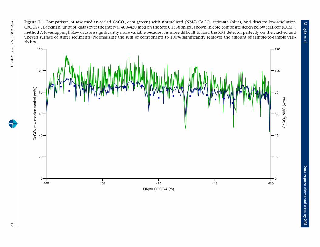
median-scaled data is the porosity effect. Deeper inthe sediment section, however, the raw sum (andraw peak areas) are often variable because the sedi-ment is stiffer and the core surface is cracked or suffi-ciently uneven that the X-ray detector assemblylands imperfectly (Fig. F4). Normalization minimizesthis high-frequency noise. Figure F4 shows the rawmedian-scaled CaCO3 and the NMS CaCO3 in adeeper section of the Site U1338 splice (Table T2).Scaling and normalization reduced what appears tobe noise in the measurement and made the totalrange more similar to the variability in the low-reso-lution CaCO3 record (Lyle and Backman, submit-ted).

The scaling and normalization process in this datareport provides a way to develop a quantitative esti-mate of sediment concentration based on XRF scans.However, one should always be aware that XRF esti-mates can have significant errors if the model of sed-iment composition used is seriously awry (e.g., thatthe “type” sediment composition used is signifi-cantly different from actual sediment composition).Another source of significant error can occur if themodel sediment components don’t match those ofthe sediment or if a major element found in the sed-iments is not included in the model. However, de-spite these issues, NMS data are significantly betterto study the changes in sediment composition thanraw XRF peak area. Raw peak area data can have evenlarger relative errors resulting from significant differ-ences in porosity between sediment layers or fromtechnical problems landing the detector on a flatsediment surface.

Example calibration of data: BaSO4

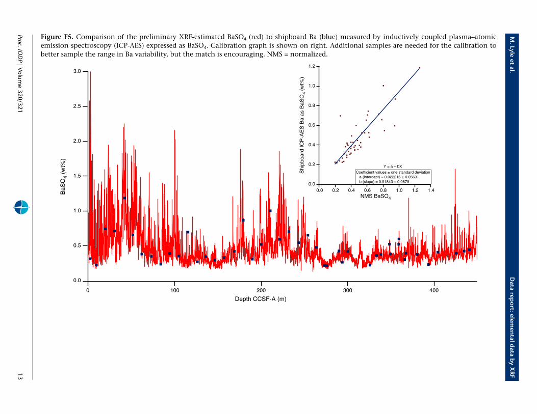
A final step—calibration with chemical analyses ofthe sediments—is required in order to properly esti-mate chemical composition with XRF. Figure F5 il-lustrates the basic process with shipboard Ba data,comparing the XRF BaSO4 estimate from the prelimi-nary linear calibration with the shipboard measure-ments. The shipboard data set is not ideal for thiscalibration because the shipboard and XRF data wereoften measured on different holes but matched bythe common meters composite depth used to buildthe splice. Nonlinear distortions of adjacent sedi-ment columns, either by coring or local sedimenta-tion variability, add noise to the calibration bymatching samples at different sediment horizons(Hagelberg et al., 1995). Compositional differencesmay actually exist between the shipboard ICP-AESand XRF NMS data that we used for the initial test

Proc. IODP | Volume 320/321

calibrations. Also, we did not have a sufficient num-ber of samples to reserve some for a test data set todetermine errors. Nevertheless, the correlation be-tween the shipboard ICP-AES data and XRF Ba data isreasonably good and will be improved by measuringmore samples along the splice.

A better example calibration exists for CaCO3 data(Lyle and Backman, submitted). Lyle and Backmanuse an extensive discrete CaCO3 data set to calibratean XRF CaCO3 estimate. Only half of the data areused for the calibration. A reserved half of the dataset is used to assess the quality of the calibration. Re-serving data allowed Lyle and Backman to show thatthe CaCO3 estimate agreed with the measuredCaCO3 by ±5 wt% (1 standard deviation).

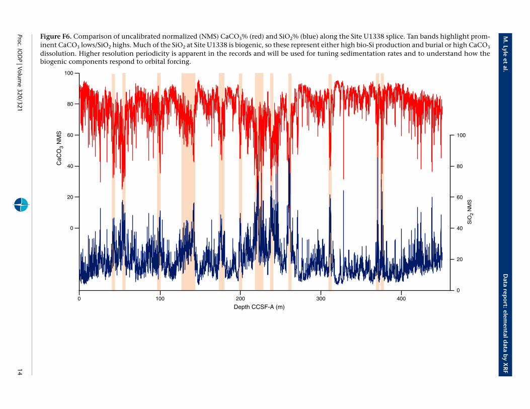
Results and discussionOne of the important uses of XRF scanning is to beable to produce high-resolution data sets of chemicalcomposition for long time spans (e.g., the 18 m.y.sediment record at Site U1338). Figure F6 showsNMS time series of CaCO3 and SiO2. These two com-ponents average ~90% of the total sediment compo-sition. Multiple intervals of low carbonate at SiteU1338 are marked by tan bars on Figure F6. Each ofthese intervals have high SiO2, caused by either thedissolution loss of carbonate from the sediment col-umn or by the very fast deposition of an SiO2-richsediment component, like the late Miocene–Pliocenediatom mat deposits found in the eastern equatorialPacific (Kemp and Baldauf, 1993; Expedition 320/321 Scientists, 2010b). One of the primary tasks ofpostexpedition studies is to understand how primaryproductivity and dissolution during early diagenesishave shaped the composition of the sediment col-umn. Based on an average sedimentation rate of 25–30 m/m.y. below 60 revised meters composite depth(rmcd) in Site U1338 (see the “Site U1338” chapter[Expedition 320/321 Scientists, 2010b]) large-scalelow weight percent CaCO3 transients are spaced amillion or more years apart. Smaller scale CaCO3

variability is also observed at all the typical orbitalforcing periods—400 to 19 k.y.

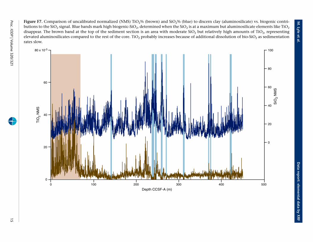
One way to study the aluminosilicate signal is withan aluminosilicate element like Ti. Because of lowlevels of aluminosilicates in the biogenic-rich equa-torial Pacific sediments, it is more appropriate to useTi than Al, because sufficient Al can be bound to bio-SiO2 to cause an appreciable Al signal, especially atintervals in the sediment column where bio-SiO2 wasinitially deposited at the seafloor but then partly dis-solved during early diagenesis (Dymond et al., 1997).Figure F7 is a plot of TiO2 and SiO2 NMS concentra-

5

M. Lyle et al. Data report: elemental data by XRF

tions along the Site U1338 splice. The blue intervalsmark intervals where SiO2 is very high but TiO2 is es-sentially zero. These sediment intervals are ex-tremely rich in bio-SiO2. In the upper 60 m of thesediment column (tan interval), we observe higherTiO2 associated with moderate SiO2, indicating rela-tively more clays. This interval marks the last 5 m.y.of the record as the site moved north of 1.3°N to itspresent position at 2.6°N. The increase in clay com-ponent may represent increased dissolution of bio-SiO2 and CaCO3 as sedimentation slowed downwhen Site U1338 moved away from the equatorialhigh-productivity zone or increased dust depositionas Site U1338 moves toward the Intertropical Con-vergence Zone. The interval of elevated Ti coincideswith the upper section of core with lower sedimenta-tion rates (12.7 m/m.y. versus 28.7 m/m.y. below; seeFig. F14 in the “Site U1338” chapter [Expedition320/321 Scientists, 2010b]). Mass accumulation ratesof TiO2, based on preliminary linear sedimentationrates, do not change with the increase in TiO2%. Thelack in change of flux makes the biogenic sedimentdissolution hypothesis the most probable cause forTiO2 enrichment in the upper section, not higherdust deposition. Supporting this interpretation, themodern position of Site U1338 is well south of thedust maximum associated with the IntertropicalConvergence Zone, 5°–6° N since 5 Ma (Hovan,1995).

ConclusionsWe present scanning XRF data along the splice ofSite U1338 (21,000 total sample measurements, with17,000 along the splice) and show their use to ex-plore the history of the equatorial Pacific productiv-ity zone. We found that we could scan the SiteU1338 splice in a reasonably short amount of time,averaging a little over 1 h apiece to scan ~250 sec-tions along the Site U1338 splice for Al, Si, K, Ca, Ti,Mn, Fe, and Ba. Raw data are a volume measure-ment, however, and must be scaled, normalized, andeventually calibrated to make an estimate of sedi-ment composition. The NMS data reduction processwe describe helps to make correlations between rawpeak areas and measured chemical compositionsmore linear so that calibration is easier. To achievegood results, care must be taken to choose a sedi-ment compositional model (median compositionand type of sediment components) that is similar tothe sediments under analysis. Calibration is the finalstep to convert XRF scan data to a compositional es-timate. Ideally, sufficient numbers of samples are

Proc. IODP | Volume 320/321

measured by other analytical methods that some ofthe data are left out of the calibration and can beused as check data.

AcknowledgmentsWe thank IODP Expedition 320/321 party members,IODP, and the IODP Gulf Coast Repository (GCR) forproviding samples and data for this report and for allthe effort they put in to properly collect and archivethe Site U1338 sediment cores. We also acknowledgethe Ocean Drilling and Sustainable Earth Sciences(ODASES) program at Texas A&M University for ac-quiring the Avaatech XRF scanner for the GCR. Scan-ning and analysis were paid for by a USAC postcruisegrant and by NSF grant OCE-0962184 to ML andAOL. TW was funded by the Deutsche Forschungsge-meinschaft (DFG)-Leibniz Center for Surface Processand Climate Studies at the University of Potsdam.

ReferencesDymond, J., 1981. Geochemistry of Nazca plate surface

sediments: an evaluation of hydrothermal, biogenic, detrital, and hydrogenous sources. In Kulm, L.D., Dymond, J., Dasch, E.J., Hussong, D.M., and Roderick, R. (Eds.), Nazca Plate: Crustal Formation and Andean Con-vergence. Mem.—Geol. Soc. Am., 154:133–173.

Dymond, J., Collier, R., McManus, J., Honjo, S., and Man-ganini, S., 1997. Can the aluminum and titanium con-tents of ocean sediments be used to determine the paleoproductivity of the oceans? Paleoceanography, 12(4):586–593. doi:10.1029/97PA01135

Expedition 320/321 Scientists, 2010a. Methods. In Pälike, H., Lyle, M., Nishi, H., Raffi, I., Gamage, K., Klaus, A., and the Expedition 320/321 Scientists, Proc. IODP, 320/321: Tokyo (Integrated Ocean Drilling Program Manage-ment International, Inc.). doi:10.2204/iodp.proc.320321.102.2010

Expedition 320/321 Scientists, 2010b. Site U1338. In Pälike, H., Lyle, M., Nishi, H., Raffi, I., Gamage, K., Klaus, A., and the Expedition 320/321 Scientists, Proc. IODP, 320/321: Tokyo (Integrated Ocean Drilling Pro-gram Management International, Inc.). doi:10.2204/iodp.proc.320321.110.2010

Hagelberg, T.K., Pisias, N.G., Mayer, L.A., Shackleton, N.J., and Mix, A.C., 1995. Spatial and temporal variability of late Neogene equatorial Pacific carbonate: Leg 138. In Pisias, N.G., Mayer, L.A., Janecek, T.R., Palmer-Julson, A., and van Andel, T.H. (Eds.), Proc. ODP, Sci Results, 138: College Station, TX (Ocean Drilling Program), 321–336. doi:10.2973/odp.proc.sr.138.116.1995

Hovan, S.A., 1995. Late Cenozoic atmospheric circulation intensity and climatic history recorded by eolian depo-sition in the eastern equatorial Pacific Ocean, Leg 138.

6

M. Lyle et al. Data report: elemental data by XRF

In Pisias, N.G., Mayer, L.A., Janecek, T.R., Palmer-Julson, A., and van Andel, T.H. (Eds.), Proc. ODP, Sci. Results, 138: College Station, TX (Ocean Drilling Program), 615–625. doi:10.2973/odp.proc.sr.138.132.1995

Jansen, J.H.F., Van der Gaast, S.J., Koster, B., and Vaars, A.J., 1998. CORTEX, a shipboard XRF-scanner for element analyses in split sediment cores. Mar. Geol., 151(1–4):143–153. doi:10.1016/S0025-3227(98)00074-7

Kemp, A.E.S., and Baldauf, J.G., 1993. Vast Neogene lami-nated diatom mat deposits from the eastern equatorial Pacific Ocean. Nature (London, U. K.), 362(6416):141–144. doi:10.1038/362141a0

Lyle, M., and Backman, J., submitted. Data report: calibra-tion of XRF-estimated CaCO3 along the Site U1338 splice. In Pälike, H., Lyle, M., Nishi, H., Raffi, I., Gam-age, K., Klaus, A., and the Expedition 320/321 Scientists, Proc. IODP, 320/321: Tokyo (Integrated Ocean Drilling Program Management International, Inc.).

Mayer, L.A., Shipley, T.H., Theyer, F., Wilkens, R.H., and Winterer, E.L., 1985. Seismic modeling and paleocean-ography at Deep Sea Drilling Project Site 574. In Mayer, L., Theyer, F., Thomas, E., et al., Init. Repts. DSDP, 85: Washington, DC (U.S. Govt. Printing Office), 947–970. doi:10.2973/dsdp.proc.85.132.1985

Mayer, L.A., Shipley, T.H., and Winterer, E.L., 1986. Equa-torial Pacific seismic reflectors as indicators of global oceanographic events. Science, 233(4765):761–764. doi:10.1126/science.233.4765.761

Richter, T.O., van der Gaast, S., Koster, B., Vaars, A., Gieles, R., de Stigter, H.C., De Haas, H., and van Weering,

Proc. IODP | Volume 320/321

T.C.E., 2006. The Avaatech XRF Core Scanner: technical description and applications to NE Atlantic sediments. In Rothwell, R.G. (Ed.), New Techniques in Sediment Core Analysis. Geol. Soc. Spec. Publ., 267(1):39–50. doi:10.1144/GSL.SP.2006.267.01.03

Tjallingii, R., Röhl, U., Kölling, M., and Bickert, T., 2007. Influence of the water content on X-ray fluorescence core-scanning measurements in soft marine sediments. Geochem., Geophys., Geosyst., 8(2):Q02004. doi:10.1029/2006GC001393

Tominaga, M., Lyle, M., and Mitchell, N.C., 2011. Seismic interpretation of pelagic sedimentation regimes in the 18–53 Ma eastern equatorial Pacific: basin-scale sedi-mentation and infilling of abyssal valleys. Geochem., Geophys., Geosyst., 12(3):Q03004. doi:10.1029/2010GC003347

Weltje, G.J., and Tjallingii, R., 2008. Calibration of XRF core scanners for quantitative geochemical logging of sediment cores: theory and application. Earth Planet. Sci. Lett., 274(3–4):423–438. doi:10.1016/j.epsl.2008.07.054

Westerhold, T., and Röhl, U., 2009. High resolution cyclo-stratigraphy of the early Eocene—new insights into the origin of the Cenozoic cooling trend. Clim. Past, 5(3):309–327. doi:10.5194/cp-5-309-2009

Initial receipt: 2 September 2011Acceptance: 1 November 2011Publication: 29 February 2012MS 320321-203

7

M. Lyle et al. Data report: elemental data by XRF

Figure F1. (A) Site map and (B) swath bathymetry map of Site U1338, located on 18 Ma crust formed at theEast Pacific Rise (from the “Site U1338” chapter [Expedition 320/321 Scientists, 2010b]). Plate tectonicmovement of the Pacific plate carried Site U1338 within 0.5° of the Equator between 13 and 8 Ma.

A

118°00'W 117°50'

10 km

35500

35600

35700

35800

35900

36000

36100

36200

36300

36400

3650

0

36600

36700

36800

36900

37000

3710037200

37300

37400

37500

3760

0

37700

37800

37900

38000

38100

38200

38300

38400

38500

Line 1

Line 3

Line 5

Line 2

Line 4

Line 6

Site U1338 (PEAT-8D)

Alternate SitePEAT-8C

4400 4200 4000 3800Depth (km)

2°40'N

2°30'

B

160°W 150° 140° 130° 120° 110°

20°S

10°

0°

10°

20°

30°N

1000 km

6 5 4 3 2

Water depth (km)

4041

42

43

67

69 70

71

72

73

74

75

76

77

78

79 81

159160

161

162

163

315

316

318

470

471472

477478479480481

571

573

574

575

597 598 599 600601

602

8423

848

849850

851852

1010

1215

1216

1217

1219

1220

1221

1222

1223

1224

1225

1243

1218

Honolulu, HawaiiMolokai F.Z.

Clarion F.Z.

Clipperton F.Z.

Galapagos F.Z.

Marquesas F.Z.

Site U1331Site U1332 Site U1333

Site U1338Site U1337

Site U1336Site U1335

Site U1334

Papeete, Tahiti

Proc. IODP | Volume 320/321 8

M. Lyle et al.

Data rep

ort: elem

ental d

ata by X

RF

Proc. IOD

P | Volume 320/321

9

ared to gamma ray attenuation (GRA) bulk density along the Site U1338d B (compressed), showing the correlation between wet bulk density andsurement and fluorescent X-ray returns depend on the total mass in the

1.2

1.4

1.6

1.8

2

0 250 300 350 400

GR

A b

ulk

dens

ity

CSF-B (m)

Figure F2. Raw sum of XRF-estimated sedimentary components compsplice, reported in core composite depth below seafloor (CCSF), methothe sum. The correlation exists because XRF scanning is a volume meavolume, which is related to the wet bulk density.

0

20

40

60

80

100

120

0 50 100 150 20

Raw sum of scaled medians, XRF composition

GRA wet bulk density

Raw

sum

of s

cale

d m

edia

ns (

%)

Depth C

M. Lyle et al.

Data rep

ort: elem

ental d

ata by X

RF

Proc. IOD

P | Volume 320/321

10

ct of different detectors. A. Al andd line) vs. 2 mA and 20 s live time

1600140012001000800

in section (mm)

600 x 1

550

500

450

400

350

300

250

200

600 x 103500400

A 20 s

one standard deviation

0211

a + bX

Figure F3. XRF scans run at two different tube currents to show the effect of power on peak areas and the effeFe scans at the Gulf Coast Repository (GCR) for Section 321-U1337A-12H-2 using 0.5 mA and 30 s live time (re(blue line). Top plots in each shows a scatter plot of the individual samples. (Continued on next page.)

2500

2000

1500

1000

500

0

Al p

eak

area

0.5

mA

30

s

16001400120010008006004002000

Depth in section (mm)

6000

5000

4000

3000

2000

1000

Al p

eak

area

2 m

A 2

0 s

2500

2000

1500

1000

500

0

Al p

eak

area

0.5

mA

30

s

6000500040003000200010000

Al peak area 2 mA 20 s

Coefficient values ± one standard deviationa = 131.17 ± 80.1b = 0.37153 ± 0.0244

Y = a + bX

240 x 103

220

200

180

160

140

120

100

Fe

peak

are

a 0

.5 m

A 3

0 s

6004002000

Depth

250 x 103

200

150

100

50

03002001000

Fe peak area 2 m

Coefficient values ±a = 6524.6 ± 859b = 0.39171 ± 0.0

Y =

Fe

peak

are

a 0.

5 m

A 3

0 s

GCR, 2 power settings

U1337A-12H-2Al

U1337A-12H-2Fe

A

M. Lyle et al.

Data rep

ort: elem

ental d

ata by X

RF

Proc. IOD

P | Volume 320/321

11

with tube current of 0.12 mA and and 20 s live time (blue line). Theppreciably affect the shape of the

115.5115.0114.5114.0

depth (mbsf)

1000 x 103

800

600

400

200

0

Fe

peak

are

a G

CR

2m

A 2

0 s

1000 x 103800

± one standard deviation

0.000228

= a + bX

U1333C-14H-4, 5Fe

Figure F3 (continued). B. Al and Fe scans comparing the MARUM XRF 3 Avaatech scanner (Bremen; red line)20 s live time to the scans from the Gulf Coast Repository (GCR) Avaatech scanner using a tube current of 2 mAtwo scanners have different generations of detectors with different sensitivity, but these differences did not adepth profiles. Top plots in each shows a scatter plot of the individual samples.

700

600

500

400

300

200

100

0Al p

eak

area

MA

RU

M 0

.12

mA

20

s

115.5115.0114.5114.0113.5113.0112.5112.0

Site U1333C depth (mbsf)

16 x 103

14

12

10

8

6

4

2

0

Al p

eak

area

GC

R 2

.0 m

A 2

0 s

700

600

500

400

300

200

100

0

Al p

eak

area

MA

RU

M

16 x 10314121086420

Al peak area GCR

Coefficient values ± one standard deviationa = 28.745 ± 8.22b = 0.042802 ± 0.00112

Y = a + bX

30 x 103

25

20

15

10

5

0Fe

peak

are

a M

AR

UM

0.1

2 m

A 2

0 s

113.5113.0112.5112.0

Site U1333C

30 x 103

25

20

15

10

5

0

Fe

peak

are

a M

AR

UM

6004002000

Fe peak area GCR

Coefficient valuesa = 125.1 ± 94.4b = 0.030486 ±

Y

GCR and MARUM, 2 power settings

U1333C-14H-4, 5Al

B

M. Lyle et al.

Data rep

ort: elem

ental d

ata by X

RF

Proc. IOD

P | Volume 320/321

12

) CaCO3 estimate (blue), and discrete low-resolutionshown in core composite depth below seafloor (CCSF),t to land the XRF detector perfectly on the cracked andcantly removes the amount of sample-to-sample vari-

420415

120

100

80

60

40

20

0

CaC

O3

NM

S (

wt%

)

Figure F4. Comparison of raw median-scaled CaCO3 data (green) with normalized (NMSCaCO3 (J. Backman, unpubl. data) over the interval 400–420 mcd on the Site U1338 splice, method A (overlapping). Raw data are significantly more variable because it is more difficuluneven surface of stiffer sediments. Normalizing the sum of components to 100% signifiability.

120

100

80

60

40

20

0

CaC

O3

raw

med

ian-

scal

ed (

wt%

)

410405400

Depth CCSF-A (m)

M. Lyle et al.

Data rep

ort: elem

ental d

ata by X

RF

Proc. IOD

P | Volume 320/321

13

a (blue) measured by inductively coupled plasma–atomicight. Additional samples are needed for the calibration toized.

400300

2

0

8

6

4

2

01.41.21.00.80.60.40.20.0

NMS BaSO4

Coefficient values ± one standard deviationa (intercept) = 0.022216 ± 0.0563b (slope) = 0.91843 ± 0.0879

Y = a + bX

Figure F5. Comparison of the preliminary XRF-estimated BaSO4 (red) to shipboard Bemission spectroscopy (ICP-AES) expressed as BaSO4. Calibration graph is shown on rbetter sample the range in Ba variability, but the match is encouraging. NMS = normal

2001000

Depth CCSF-A (m)

3.0

2.5

2.0

1.5

1.0

0.5

0.0

BaS

O4

(wt%

)1.

1.

0.

0.

0.

0.

0.

Shi

pboa

rd IC

P-A

ES

Ba

as B

aSO

4 (w

t%)

M. Lyle et al.

Data rep

ort: elem

ental d

ata by X

RF

Proc. IOD

P | Volume 320/321

14

along the Site U1338 splice. Tan bands highlight prom- either high bio-Si production and burial or high CaCO3

uning sedimentation rates and to understand how the

40000

100

80

60

40

20

0

SiO

2 N

MS

Figure F6. Comparison of uncalibrated normalized (NMS) CaCO3% (red) and SiO2% (blue) inent CaCO3 lows/SiO2 highs. Much of the SiO2 at Site U1338 is biogenic, so these representdissolution. Higher resolution periodicity is apparent in the records and will be used for tbiogenic components respond to orbital forcing.

100

80

60

40

20

0

CaC

O3

NM

S

32001000

Depth CCSF-A (m)

M. Lyle et al.

Data rep

ort: elem

ental d

ata by X

RF

Proc. IOD

P | Volume 320/321

15

o discern clay (aluminosilicate) vs. biogenic contri- a maximum but aluminosilicate elements like TiO2

but relatively high amounts of TiO2, representingadditional dissolution of bio-SiO2 as sedimentation

500400

100

80

60

40

20

0

SiO

2 N

MS

Figure F7. Comparison of uncalibrated normalized (NMS) TiO2% (brown) and SiO2% (blue) tbutions to the SiO2 signal. Blue bands mark high biogenic-SiO2, determined when the SiO2 is atdisappear. The brown band at the top of the sediment section is an area with moderate SiO2

elevated aluminosilicates compared to the rest of the core. TiO2 probably increases because of rates slow.

80 x 10-3

60

40

20

0

TiO

2 N

MS

3002001000

Depth CCSF-A (m)

M. Lyle et al.

Data rep

ort: elem

ental d

ata by X

RF

Proc. IOD

P | Volume 320/321

16

i, Mn, and Fe are from the 10 kV scan; Ba isNSPL.XLS in XRF in “Supplementary mate-

Mn area Fe area

Ba area(50 kVscan)

65,711 50,683 3,39814,737 90,042 12,19920,200 89,287 10,97420,278 90,977 9,94050,111 90,424 10,15816,935 94,039 9,62348,228 87,932 9,97243,363 89,331 9,66549,993 93,019 10,38213,003 87,689 9,77215,611 96,548 10,46192,678 92,263 10,61445,705 87,897 9,47140,378 91,854 10,18630,007 78,209 8,36930,953 79,233 8,85133,817 79,555 8,69231,207 70,631 8,18936,204 68,976 8,08831,918 75,054 8,45226,998 69,963 7,51519,522 70,260 7,40222,116 69,223 7,48215,466 62,797 5,85021,300 70,224 6,13917,031 55,641 5,94456,416 67,879 6,75140,821 67,904 6,69250,170 66,785 6,74234,887 59,237 7,11226,677 62,104 6,53230,073 67,662 6,62439,294 59,105 6,96757,592 65,050 6,81033,031 76,096 6,82235,152 62,327 6,85526,640 63,732 6,24322,303 71,860 7,16523,729 70,781 7,28626,194 73,703 6,21037,549 69,539 6,54156,226 67,783 6,65758,016 73,135 6,530

Table T1. Raw XRF scan peak area data for all scans on Site U1338, unspliced.

Overlaps of sections where the splice jumps to a different hole are shaded (tan = overlapping sections in splice, green = splice join). Al, Si, K, Ca, Tfrom the 50 kV scan. Only a portion of this table appears here. The complete table is available in ASCII and in Microsoft Excel format (see RAWUrial”).

Core, section

Depth in section(mm)

Measurementdate

(2009)

Depth (mbsf/CSF-A[m])

Depth (mcd/

CCSF-A[m]) Al area Si area S area Cl area K area Ca area Ti area

321-U1338A-1H-1 25 29 Jul 0.025 0.065 –196 31,096 13,457 293,730 –1,343 2,258,381 1,3201H-1 50 29 Jul 0.050 0.090 –98 39,489 27,680 771,065 7,437 2,914,316 3,180 11H-1 75 29 Jul 0.075 0.115 31 54,291 25,702 670,383 7,910 3,917,938 4,312 11H-1 100 29 Jul 0.100 0.140 –64 58,567 25,225 649,819 8,859 3,879,549 4,132 11H-1 125 29 Jul 0.125 0.165 261 74,200 21,599 559,320 8,642 5,529,714 5,545 11H-1 150 29 Jul 0.150 0.190 474 99,029 21,387 577,860 9,292 5,459,765 4,785 11H-1 175 29 Jul 0.175 0.215 294 79,255 22,413 611,799 7,209 5,622,123 5,203 11H-1 200 29 Jul 0.200 0.240 168 78,416 24,243 606,554 7,054 5,460,881 5,675 11H-1 225 29 Jul 0.225 0.265 633 106,394 21,727 570,990 7,893 5,467,310 4,459 11H-1 250 29 Jul 0.250 0.290 295 109,612 23,150 598,106 6,155 5,340,919 3,428 11H-1 275 29 Jul 0.275 0.315 165 79,464 20,977 557,697 6,094 6,125,817 4,628 21H-1 300 29 Jul 0.300 0.340 262 57,496 21,091 578,414 6,547 6,161,687 4,261 11H-1 325 29 Jul 0.325 0.365 397 55,628 23,413 622,942 6,987 5,875,783 5,0781H-1 350 29 Jul 0.350 0.390 611 63,358 21,954 591,906 7,383 6,150,193 4,3841H-1 375 29 Jul 0.375 0.415 448 59,072 21,785 612,824 5,672 5,821,063 4,4371H-1 400 29 Jul 0.400 0.440 526 56,740 22,097 612,332 6,277 5,775,173 4,2641H-1 425 29 Jul 0.425 0.465 515 59,134 21,841 627,211 5,879 6,045,124 4,1831H-1 450 29 Jul 0.450 0.490 276 49,103 23,257 640,795 6,365 5,620,226 3,9631H-1 475 29 Jul 0.475 0.515 474 40,776 24,811 707,600 5,090 5,065,880 3,1541H-1 500 29 Jul 0.500 0.540 412 42,209 26,338 718,848 6,063 5,287,877 3,7731H-1 525 29 Jul 0.525 0.565 250 43,704 23,015 668,223 5,078 5,400,234 2,6621H-1 550 29 Jul 0.550 0.590 344 65,255 22,762 656,185 5,510 5,924,826 3,7821H-1 575 29 Jul 0.575 0.615 508 55,367 23,779 649,213 4,293 5,533,030 3,1501H-1 600 29 Jul 0.600 0.640 292 54,203 22,318 622,895 2,539 5,330,983 2,9731H-1 625 29 Jul 0.625 0.665 551 69,327 21,772 604,146 3,248 6,307,831 2,8411H-1 650 29 Jul 0.650 0.690 253 67,414 24,065 655,523 3,049 5,421,827 2,3761H-1 675 29 Jul 0.675 0.715 360 57,532 22,015 617,115 4,382 5,934,125 2,8341H-1 700 29 Jul 0.700 0.740 306 57,916 21,199 611,161 3,128 5,851,201 2,7401H-1 725 29 Jul 0.725 0.765 620 62,461 20,340 571,223 4,724 6,091,732 2,7621H-1 750 29 Jul 0.750 0.790 261 44,115 20,660 629,893 2,852 5,095,266 1,7331H-1 775 29 Jul 0.775 0.815 325 49,114 18,640 574,651 1,430 5,803,417 1,9011H-1 800 29 Jul 0.800 0.840 266 54,097 20,076 636,584 2,043 5,640,361 1,8761H-1 825 29 Jul 0.825 0.865 110 48,609 22,560 622,630 1,103 4,894,580 2,2531H-1 850 29 Jul 0.850 0.890 263 70,631 22,439 616,785 3,341 5,000,849 2,5081H-1 875 29 Jul 0.875 0.915 646 77,556 21,123 596,848 4,157 6,044,992 3,0101H-1 900 29 Jul 0.900 0.940 337 62,267 20,490 605,333 882 4,777,876 3,9881H-1 925 29 Jul 0.925 0.965 47 58,742 24,689 670,855 3,681 4,745,994 1,5461H-1 950 29 Jul 0.950 0.990 400 73,213 22,566 620,576 3,830 4,834,842 1,2731H-1 975 29 Jul 0.975 1.015 350 73,781 21,954 611,750 5,517 5,119,603 2,0191H-1 1,000 29 Jul 1.000 1.040 610 89,812 19,612 539,125 4,517 5,907,522 3,2151H-1 1,025 29 Jul 1.025 1.065 544 81,524 20,710 568,607 5,489 5,312,686 2,8551H-1 1,050 29 Jul 1.050 1.090 171 60,647 22,569 607,420 3,570 4,806,630 2,4271H-1 1,075 29 Jul 1.075 1.115 –56 54,263 24,678 616,152 6,011 3,942,852 3,024

M. Lyle et al. Data report: elemental data by XRF

Table T2. Spliced NMS, Hole U1338A. (Continued on next two pages.)

Al, Si, K, Ca, Ti, Mn, and Fe, are from the 10 kV scan; Ba is from the 50 kV scan. Only a portion of this table appears here. The complete table isavailable in ASCII and in Microsoft Excel format (see NMSSPL.XLS in XRF in “Supplementary material”).

Core, section

Depthin section

(mm)

Measurementdate

(2009)

Depth (mbsf/CSF-A[m])

Depth (mcd/

CCSF-A[m])

Rawcomponent

sum (%) Al area Al median-

scaleAl2O3NMS Si area

Si median-scale

SiO2NMS S area

321-U1338A-1H-1 25 29 Jul 0.025 0.065 32.443 –196 0.000 0.000 31,096 3.04 9.38 13,457 1H-1 50 29 Jul 0.050 0.090 42.712 –98 0.000 0.000 39,489 3.86 9.04 27,680 1H-1 75 29 Jul 0.075 0.115 56.755 31 0.008 0.014 54,291 5.31 9.36 25,702 1H-1 100 29 Jul 0.100 0.140 56.684 –64 0.000 0.000 58,567 5.73 10.11 25,225 1H-1 125 29 Jul 0.125 0.165 79.203 261 0.069 0.087 74,200 7.26 9.16 21,599 1H-1 150 29 Jul 0.150 0.190 80.580 474 0.125 0.155 99,029 9.69 12.02 21,387 1H-1 175 29 Jul 0.175 0.215 80.788 294 0.078 0.096 79,255 7.75 9.60 22,413 1H-1 200 29 Jul 0.200 0.240 78.611 168 0.044 0.056 78,416 7.67 9.76 24,243 1H-1 225 29 Jul 0.225 0.265 81.680 633 0.167 0.205 106,394 10.41 12.74 21,727 1H-1 250 29 Jul 0.250 0.290 79.923 295 0.078 0.098 109,612 10.72 13.42 23,150 1H-1 275 29 Jul 0.275 0.315 87.682 165 0.044 0.050 79,464 7.77 8.87 20,977 1H-1 300 29 Jul 0.300 0.340 85.808 262 0.069 0.081 57,496 5.62 6.55 21,091 1H-1 325 29 Jul 0.325 0.365 80.863 397 0.105 0.130 55,628 5.44 6.73 23,413 1H-1 350 29 Jul 0.350 0.390 85.145 611 0.161 0.190 63,358 6.20 7.28 21,954 1H-1 375 29 Jul 0.375 0.415 80.249 448 0.118 0.148 59,072 5.78 7.20 21,785 1H-1 400 29 Jul 0.400 0.440 79.514 526 0.139 0.175 56,740 5.55 6.98 22,097 1H-1 425 29 Jul 0.425 0.465 83.140 515 0.136 0.164 59,134 5.78 6.96 21,841 1H-1 450 29 Jul 0.450 0.490 76.661 276 0.073 0.095 49,103 4.80 6.27 23,257 1H-1 475 29 Jul 0.475 0.515 68.939 474 0.125 0.182 40,776 3.99 5.79 24,811 1H-1 500 29 Jul 0.500 0.540 71.903 412 0.109 0.151 42,209 4.13 5.74 26,338 1H-1 525 29 Jul 0.525 0.565 73.274 250 0.066 0.090 43,704 4.28 5.83 23,015 1H-1 550 29 Jul 0.550 0.590 81.936 344 0.091 0.111 65,255 6.38 7.79 22,762 1H-1 575 29 Jul 0.575 0.615 76.084 508 0.134 0.176 55,367 5.42 7.12 23,779 1H-1 600 29 Jul 0.600 0.640 73.171 292 0.077 0.105 54,203 5.30 7.25 22,318 1H-1 625 29 Jul 0.625 0.665 87.105 551 0.146 0.167 69,327 6.78 7.79 21,772 1H-1 650 29 Jul 0.650 0.690 75.556 253 0.067 0.088 67,414 6.59 8.73 24,065 1H-1 675 29 Jul 0.675 0.715 81.516 360 0.095 0.117 57,532 5.63 6.90 22,015 1H-1 700 29 Jul 0.700 0.740 80.348 306 0.081 0.101 57,916 5.67 7.05 21,199 1H-1 725 29 Jul 0.725 0.765 83.993 620 0.164 0.195 62,461 6.11 7.27 20,340 1H-1 750 29 Jul 0.750 0.790 69.393 261 0.069 0.099 44,115 4.32 6.22 20,660 1H-1 775 29 Jul 0.775 0.815 78.685 325 0.086 0.109 49,114 4.80 6.11 18,640 1H-1 800 29 Jul 0.800 0.840 77.206 266 0.070 0.091 54,097 5.29 6.85 20,076 1H-1 825 29 Jul 0.825 0.865 67.264 110 0.029 0.043 48,609 4.75 7.07 22,560 1H-1 850 29 Jul 0.850 0.890 71.032 263 0.070 0.098 70,631 6.91 9.73 22,439 1H-1 875 29 Jul 0.875 0.915 84.829 646 0.171 0.201 77,556 7.59 8.94 21,123 1H-1 900 29 Jul 0.900 0.940 67.185 337 0.089 0.133 62,267 6.09 9.07 20,490 1H-1 925 29 Jul 0.925 0.965 66.351 47 0.012 0.019 58,742 5.75 8.66 24,689 1H-1 950 29 Jul 0.950 0.990 69.048 400 0.106 0.153 73,213 7.16 10.37 22,566 1H-1 975 29 Jul 0.975 1.015 72.707 350 0.092 0.127 73,781 7.22 9.93 21,954 1H-1 1,000 29 Jul 1.000 1.040 84.207 610 0.161 0.191 89,812 8.79 10.43 19,612 1H-1 1,025 29 Jul 1.025 1.065 76.006 544 0.144 0.189 81,524 7.97 10.49 20,710 1H-1 1,050 29 Jul 1.050 1.090 67.609 171 0.045 0.067 60,647 5.93 8.77 22,569 1H-1 1,075 29 Jul 1.075 1.115 56.223 –56 0.000 0.000 54,263 5.31 9.44 24,678 1H-1 1,100 29 Jul 1.100 1.140 45.720 –127 0.000 0.000 45,904 4.49 9.82 24,823 1H-1 1,125 29 Jul 1.125 1.165 62.460 4 0.001 0.002 79,860 7.81 12.51 24,486 1H-1 1,150 29 Jul 1.150 1.190 48.900 117 0.031 0.063 56,342 5.51 11.27 20,845 1H-1 1,175 29 Jul 1.175 1.215 54.956 182 0.048 0.088 79,743 7.80 14.19 30,302 1H-1 1,200 29 Jul 1.200 1.240 49.787 195 0.052 0.104 71,091 6.95 13.97 31,844 1H-1 1,225 29 Jul 1.225 1.265 54.761 104 0.027 0.050 74,635 7.30 13.33 25,977 1H-1 1,250 29 Jul 1.250 1.290 35.408 –331 0.000 0.000 45,485 4.45 12.57 31,332 1H-1 1,275 29 Jul 1.275 1.315 45.565 430 0.114 0.249 107,283 10.49 23.03 35,849 1H-1 1,300 29 Jul 1.300 1.340 26.109 –169 0.000 0.000 37,894 3.71 14.20 33,187 1H-1 1,325 29 Jul 1.325 1.365 33.589 –38 0.000 0.000 58,964 5.77 17.17 29,457 1H-1 1,350 29 Jul 1.350 1.390 39.756 –262 0.000 0.000 51,970 5.08 12.79 34,524 1H-1 1,375 29 Jul 1.375 1.415 35.315 –332 0.000 0.000 54,052 5.29 14.97 33,412 1H-1 1,400 29 Jul 1.400 1.440 43.730 –37 0.000 0.000 72,746 7.12 16.27 31,160 1H-1 1,425 29 Jul 1.425 1.465 46.225 336 0.089 0.192 88,308 8.64 18.69 27,293 1H-2 25 29 Jul 1.525 1.565 29.196 –146 0.000 0.000 59,620 5.83 19.98 26,096 1H-2 50 29 Jul 1.550 1.590 34.848 –349 0.000 0.000 42,906 4.20 12.04 32,993 1H-2 75 29 Jul 1.575 1.615 27.605 –272 0.000 0.000 26,424 2.58 9.36 32,931 1H-2 100 29 Jul 1.600 1.640 26.098 –251 0.000 0.000 30,607 2.99 11.47 32,628 1H-2 125 29 Jul 1.625 1.665 24.268 –176 0.000 0.000 35,143 3.44 14.17 30,839

Proc. IODP | Volume 320/321 17

M. Lyle et al. Data report: elemental data by XRF

Table T2 (continued). (Continued on next page.)

Core, section

Depthin section

(mm) Cl area K area K median-

scaleK2O NMS Ca area

Ca median-scale

CaCO3NMS Ti area

Ti median-scale

TiO2 NMS Mn area

Mn median-

scale

321-U1338A-1H-1 25 293,730 (1,343) 0.000 0.000 2,258,381 28.32 87.28 1,320 0.0011 0.0033 65,711 0.5111H-1 50 771,065 7,437 0.172 0.403 2,914,316 36.54 85.55 3,180 0.0026 0.0060 114,737 0.8931H-1 75 670,383 7,910 0.183 0.323 3,917,938 49.12 86.56 4,312 0.0035 0.0061 120,200 0.9351H-1 100 649,819 8,859 0.205 0.362 3,879,549 48.64 85.82 4,132 0.0033 0.0059 120,278 0.9361H-1 125 559,320 8,642 0.200 0.253 5,529,714 69.33 87.54 5,545 0.0045 0.0056 150,111 1.1681H-1 150 577,860 9,292 0.215 0.267 5,459,765 68.46 84.95 4,785 0.0038 0.0048 116,935 0.9101H-1 175 611,799 7,209 0.167 0.207 5,622,123 70.49 87.26 5,203 0.0042 0.0052 148,228 1.1531H-1 200 606,554 7,054 0.163 0.208 5,460,881 68.47 87.10 5,675 0.0046 0.0058 143,363 1.1151H-1 225 570,990 7,893 0.183 0.224 5,467,310 68.55 83.93 4,459 0.0036 0.0044 149,993 1.1671H-1 250 598,106 6,155 0.143 0.178 5,340,919 66.97 83.79 3,428 0.0028 0.0034 113,003 0.8791H-1 275 557,697 6,094 0.141 0.161 6,125,817 76.81 87.60 4,628 0.0037 0.0042 215,611 1.6781H-1 300 578,414 6,547 0.152 0.177 6,161,687 77.26 90.04 4,261 0.0034 0.0040 192,678 1.4991H-1 325 622,942 6,987 0.162 0.200 5,875,783 73.67 91.11 5,078 0.0041 0.0050 45,705 0.3561H-1 350 591,906 7,383 0.171 0.201 6,150,193 77.11 90.57 4,384 0.0035 0.0041 40,378 0.3141H-1 375 612,824 5,672 0.131 0.164 5,821,063 72.99 90.95 4,437 0.0036 0.0044 30,007 0.2331H-1 400 612,332 6,277 0.145 0.183 5,775,173 72.41 91.07 4,264 0.0034 0.0043 30,953 0.2411H-1 425 627,211 5,879 0.136 0.164 6,045,124 75.80 91.17 4,183 0.0034 0.0040 33,817 0.2631H-1 450 640,795 6,365 0.147 0.192 5,620,226 70.47 91.92 3,963 0.0032 0.0042 31,207 0.2431H-1 475 707,600 5,090 0.118 0.171 5,065,880 63.52 92.14 3,154 0.0025 0.0037 36,204 0.2821H-1 500 718,848 6,063 0.140 0.195 5,287,877 66.30 92.21 3,773 0.0030 0.0042 31,918 0.2481H-1 525 668,223 5,078 0.118 0.160 5,400,234 67.71 92.41 2,662 0.0021 0.0029 26,998 0.2101H-1 550 656,185 5,510 0.128 0.156 5,924,826 74.29 90.67 3,782 0.0030 0.0037 19,522 0.1521H-1 575 649,213 4,293 0.099 0.131 5,533,030 69.38 91.18 3,150 0.0025 0.0033 22,116 0.1721H-1 600 622,895 2,539 0.059 0.080 5,330,983 66.84 91.35 2,973 0.0024 0.0033 15,466 0.1201H-1 625 604,146 3,248 0.075 0.086 6,307,831 79.09 90.80 2,841 0.0023 0.0026 21,300 0.1661H-1 650 655,523 3,049 0.071 0.093 5,421,827 67.98 89.97 2,376 0.0019 0.0025 17,031 0.1331H-1 675 617,115 4,382 0.101 0.124 5,934,125 74.40 91.28 2,834 0.0023 0.0028 56,416 0.4391H-1 700 611,161 3,128 0.072 0.090 5,851,201 73.36 91.31 2,740 0.0022 0.0027 40,821 0.3181H-1 725 571,223 4,724 0.109 0.130 6,091,732 76.38 90.94 2,762 0.0022 0.0026 50,170 0.3901H-1 750 629,893 2,852 0.066 0.095 5,095,266 63.89 92.06 1,733 0.0014 0.0020 34,887 0.2711H-1 775 574,651 1,430 0.033 0.042 5,803,417 72.77 92.48 1,901 0.0015 0.0019 26,677 0.2081H-1 800 636,584 2,043 0.047 0.061 5,640,361 70.72 91.60 1,876 0.0015 0.0020 30,073 0.2341H-1 825 622,630 1,103 0.026 0.038 4,894,580 61.37 91.24 2,253 0.0018 0.0027 39,294 0.3061H-1 850 616,785 3,341 0.077 0.109 5,000,849 62.70 88.27 2,508 0.0020 0.0028 57,592 0.4481H-1 875 596,848 4,157 0.096 0.113 6,044,992 75.79 89.35 3,010 0.0024 0.0029 33,031 0.2571H-1 900 605,333 882 0.020 0.030 4,777,876 59.91 89.17 3,988 0.0032 0.0048 35,152 0.2741H-1 925 670,855 3,681 0.085 0.128 4,745,994 59.51 89.69 1,546 0.0012 0.0019 26,640 0.2071H-1 950 620,576 3,830 0.089 0.128 4,834,842 60.62 87.79 1,273 0.0010 0.0015 22,303 0.1741H-1 975 611,750 5,517 0.128 0.176 5,119,603 64.19 88.29 2,019 0.0016 0.0022 23,729 0.1851H-1 1,000 539,125 4,517 0.105 0.124 5,907,522 74.07 87.96 3,215 0.0026 0.0031 26,194 0.2041H-1 1,025 568,607 5,489 0.127 0.167 5,312,686 66.61 87.64 2,855 0.0023 0.0030 37,549 0.2921H-1 1,050 607,420 3,570 0.083 0.122 4,806,630 60.27 89.14 2,427 0.0019 0.0029 56,226 0.4371H-1 1,075 616,152 6,011 0.139 0.248 3,942,852 49.44 87.93 3,024 0.0024 0.0043 58,016 0.4511H-1 1,100 668,021 4,239 0.098 0.215 3,198,341 40.10 87.71 1,676 0.0013 0.0029 38,598 0.3001H-1 1,125 621,320 8,279 0.192 0.307 4,216,530 52.87 84.64 4,523 0.0036 0.0058 75,124 0.5851H-1 1,150 510,676 3,212 0.074 0.152 3,360,285 42.13 86.16 4,060 0.0033 0.0067 35,604 0.2771H-1 1,175 724,966 14,248 0.330 0.600 3,577,836 44.86 81.63 4,674 0.0038 0.0068 69,903 0.5441H-1 1,200 721,878 7,842 0.182 0.365 3,306,120 41.45 83.26 3,188 0.0026 0.0051 34,079 0.2651H-1 1,225 643,154 12,751 0.295 0.539 3,618,646 45.37 82.85 3,744 0.0030 0.0055 53,209 0.4141H-1 1,250 753,138 12,815 0.297 0.838 2,292,403 28.74 81.18 4,540 0.0036 0.0103 39,202 0.3051H-1 1,275 770,154 14,936 0.346 0.759 2,644,121 33.15 72.76 4,506 0.0036 0.0079 33,461 0.2601H-1 1,300 805,380 14,758 0.342 1.309 1,581,744 19.83 75.96 5,125 0.0041 0.0158 39,551 0.3081H-1 1,325 755,554 16,924 0.392 1.167 1,988,632 24.93 74.23 7,922 0.0064 0.0189 39,644 0.3081H-1 1,350 814,134 19,003 0.440 1.107 2,530,553 31.73 79.81 7,434 0.0060 0.0150 48,185 0.3751H-1 1,375 795,217 21,032 0.487 1.379 2,142,968 26.87 76.08 9,576 0.0077 0.0218 41,151 0.3201H-1 1,400 758,584 23,438 0.543 1.241 2,650,436 33.23 75.99 10,547 0.0085 0.0194 46,610 0.3631H-1 1,425 586,722 20,293 0.470 1.017 2,783,249 34.90 75.49 8,328 0.0067 0.0145 47,630 0.3711H-2 25 538,343 18,325 0.424 1.453 1,571,684 19.71 67.50 8,918 0.0072 0.0245 141,444 1.1011H-2 50 787,958 15,936 0.369 1.059 2,226,434 27.92 80.11 7,310 0.0059 0.0168 50,681 0.3941H-2 75 805,494 12,733 0.295 1.068 1,770,030 22.19 80.39 4,380 0.0035 0.0127 80,342 0.6251H-2 100 784,573 17,289 0.400 1.534 1,467,440 18.40 70.50 8,003 0.0064 0.0246 227,596 1.7711H-2 125 771,104 14,781 0.342 1.410 1,343,867 16.85 69.43 5,566 0.0045 0.0184 188,299 1.465

Proc. IODP | Volume 320/321 18

M. Lyle et al. Data report: elemental data by XRF

Table T2 (continued).

Core, section

Depthin section

(mm)MnONMS Fe area

Fe median-scale

Fe2O3NMS

Ba area(50kVscan)

Ba median-scaled

BaSO4NMS

321-U1338A-1H-1 25 1.576 50,683 0.449 1.382 3,398 0.124 0.3811H-1 50 2.090 90,042 0.797 1.865 12,199 0.444 1.0401H-1 75 1.648 89,287 0.790 1.392 10,974 0.400 0.7041H-1 100 1.651 90,977 0.805 1.420 9,940 0.362 0.6391H-1 125 1.475 90,424 0.800 1.010 10,158 0.370 0.4671H-1 150 1.129 94,039 0.832 1.033 9,623 0.350 0.4351H-1 175 1.428 87,932 0.778 0.963 9,972 0.363 0.4491H-1 200 1.419 89,331 0.791 1.006 9,665 0.352 0.4481H-1 225 1.429 93,019 0.823 1.008 10,382 0.378 0.4631H-1 250 1.100 87,689 0.776 0.971 9,772 0.356 0.4451H-1 275 1.913 96,548 0.854 0.974 10,461 0.381 0.4341H-1 300 1.747 92,263 0.816 0.951 10,614 0.386 0.4501H-1 325 0.440 87,897 0.778 0.962 9,471 0.345 0.4261H-1 350 0.369 91,854 0.813 0.955 10,186 0.371 0.4361H-1 375 0.291 78,209 0.692 0.862 8,369 0.305 0.3801H-1 400 0.303 79,233 0.701 0.882 8,851 0.322 0.4051H-1 425 0.316 79,555 0.704 0.847 8,692 0.317 0.3811H-1 450 0.317 70,631 0.625 0.815 8,189 0.298 0.3891H-1 475 0.409 68,976 0.610 0.885 8,088 0.295 0.4271H-1 500 0.345 75,054 0.664 0.924 8,452 0.308 0.4281H-1 525 0.287 69,963 0.619 0.845 7,515 0.274 0.3731H-1 550 0.185 70,260 0.622 0.759 7,402 0.270 0.3291H-1 575 0.226 69,223 0.613 0.805 7,482 0.272 0.3581H-1 600 0.164 62,797 0.556 0.759 5,850 0.213 0.2911H-1 625 0.190 70,224 0.621 0.713 6,139 0.224 0.2571H-1 650 0.175 55,641 0.492 0.652 5,944 0.216 0.2861H-1 675 0.538 67,879 0.601 0.737 6,751 0.246 0.3021H-1 700 0.395 67,904 0.601 0.748 6,692 0.244 0.3031H-1 725 0.465 66,785 0.591 0.704 6,742 0.246 0.2921H-1 750 0.391 59,237 0.524 0.755 7,112 0.259 0.3731H-1 775 0.264 62,104 0.550 0.698 6,532 0.238 0.3021H-1 800 0.303 67,662 0.599 0.776 6,624 0.241 0.3121H-1 825 0.455 59,105 0.523 0.778 6,967 0.254 0.3771H-1 850 0.631 65,050 0.576 0.810 6,810 0.248 0.3491H-1 875 0.303 76,096 0.673 0.794 6,822 0.248 0.2931H-1 900 0.407 62,327 0.552 0.821 6,855 0.250 0.3721H-1 925 0.312 63,732 0.564 0.850 6,243 0.227 0.3431H-1 950 0.251 71,860 0.636 0.921 7,165 0.261 0.3781H-1 975 0.254 70,781 0.626 0.861 7,286 0.265 0.3651H-1 1,000 0.242 73,703 0.652 0.775 6,210 0.226 0.2691H-1 1,025 0.384 69,539 0.615 0.810 6,541 0.238 0.3131H-1 1,050 0.647 67,783 0.600 0.887 6,657 0.242 0.3591H-1 1,075 0.803 73,135 0.647 1.151 6,530 0.238 0.4231H-1 1,100 0.657 53,512 0.474 1.036 6,996 0.255 0.5571H-1 1,125 0.936 81,515 0.721 1.155 7,629 0.278 0.4451H-1 1,150 0.567 72,320 0.640 1.309 6,332 0.231 0.4721H-1 1,175 0.990 113,512 1.004 1.828 10,023 0.365 0.6641H-1 1,200 0.533 66,715 0.590 1.186 7,926 0.289 0.5801H-1 1,225 0.756 111,562 0.987 1.803 9,933 0.362 0.6601H-1 1,250 0.861 127,247 1.126 3.180 13,312 0.485 1.3691H-1 1,275 0.571 104,438 0.924 2.028 7,418 0.270 0.5931H-1 1,300 1.179 148,491 1.314 5.033 16,535 0.602 2.3061H-1 1,325 0.918 176,752 1.564 4.657 16,931 0.617 1.8351H-1 1,350 0.943 179,690 1.590 4.000 14,622 0.532 1.3391H-1 1,375 0.907 198,901 1.760 4.984 16,031 0.584 1.6531H-1 1,400 0.829 210,526 1.863 4.260 16,623 0.605 1.3841H-1 1,425 0.802 153,476 1.358 2.938 10,865 0.396 0.8561H-2 25 3.770 190,726 1.688 5.781 12,023 0.438 1.5001H-2 50 1.132 163,752 1.449 4.158 14,198 0.517 1.4841H-2 75 2.265 155,479 1.376 4.984 14,498 0.528 1.9121H-2 100 6.786 203,431 1.800 6.898 19,959 0.727 2.7851H-2 125 6.037 179,374 1.587 6.541 15,976 0.582 2.397

Proc. IODP | Volume 320/321 19