Data Report of the 2007 and 2008 Yamal Expeditions: Nadym ...
133
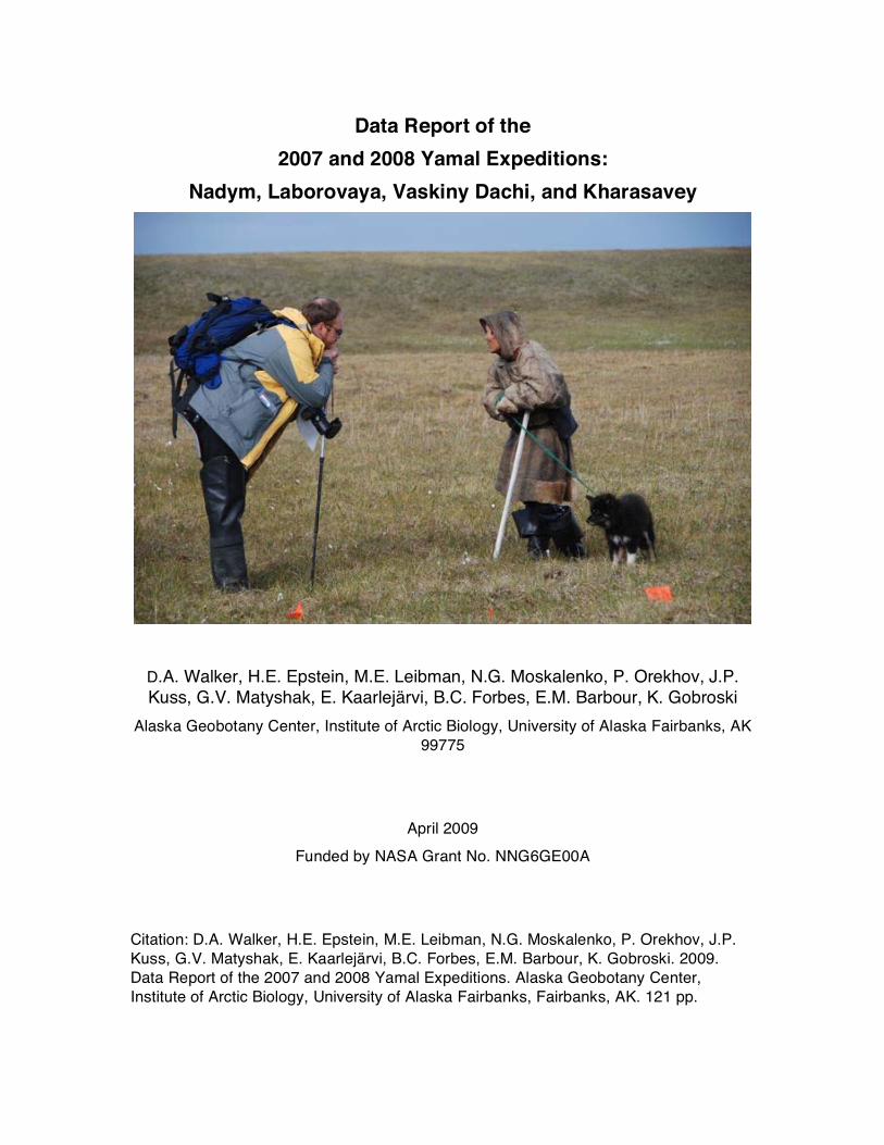
Data Report of the 2007 and 2008 Yamal Expeditions: Nadym, Laborovaya, Vaskiny Dachi, and Kharasavey D.A. Walker, H.E. Epstein, M.E. Leibman, N.G. Moskalenko, P. Orekhov, J.P. Kuss, G.V. Matyshak, E. Kaarlejärvi, B.C. Forbes, E.M. Barbour, K. Gobroski Alaska Geobotany Center, Institute of Arctic Biology, University of Alaska Fairbanks, AK 99775 April 2009 Funded by NASA Grant No. NNG6GE00A Citation: D.A. Walker, H.E. Epstein, M.E. Leibman, N.G. Moskalenko, P. Orekhov, J.P. Kuss, G.V. Matyshak, E. Kaarlejärvi, B.C. Forbes, E.M. Barbour, K. Gobroski. 2009. Data Report of the 2007 and 2008 Yamal Expeditions. Alaska Geobotany Center, Institute of Arctic Biology, University of Alaska Fairbanks, Fairbanks, AK. 121 pp.
Transcript of Data Report of the 2007 and 2008 Yamal Expeditions: Nadym ...
Data Report of the 2007 and 2008 Yamal Expeditions:
Nadym, Laborovaya, Vaskiny Dachi, and Kharasavey
D.A. Walker, H.E. Epstein, M.E. Leibman, N.G. Moskalenko, P. Orekhov, J.P. Kuss, G.V. Matyshak, E. Kaarlejärvi, B.C. Forbes, E.M. Barbour, K. Gobroski
Alaska Geobotany Center, Institute of Arctic Biology, University of Alaska Fairbanks, AK 99775
April 2009 Funded by NASA Grant No. NNG6GE00A
Citation: D.A. Walker, H.E. Epstein, M.E. Leibman, N.G. Moskalenko, P. Orekhov, J.P. Kuss, G.V. Matyshak, E. Kaarlejärvi, B.C. Forbes, E.M. Barbour, K. Gobroski. 2009. Data Report of the 2007 and 2008 Yamal Expeditions. Alaska Geobotany Center, Institute of Arctic Biology, University of Alaska Fairbanks, Fairbanks, AK. 121 pp.

2
Cover Photo: Pavel Orekhov and Nenets herder at Kharasavey, Site 1, Aug. 2009. Photo by D.A. Walker, DSC_1498.jpg.
i
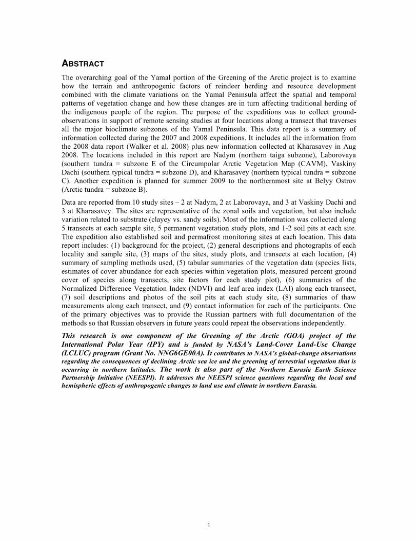
ABSTRACT The overarching goal of the Yamal portion of the Greening of the Arctic project is to examine how the terrain and anthropogenic factors of reindeer herding and resource development combined with the climate variations on the Yamal Peninsula affect the spatial and temporal patterns of vegetation change and how these changes are in turn affecting traditional herding of the indigenous people of the region. The purpose of the expeditions was to collect ground-observations in support of remote sensing studies at four locations along a transect that traverses all the major bioclimate subzones of the Yamal Peninsula. This data report is a summary of information collected during the 2007 and 2008 expeditions. It includes all the information from the 2008 data report (Walker et al. 2008) plus new information collected at Kharasavey in Aug 2008. The locations included in this report are Nadym (northern taiga subzone), Laborovaya (southern tundra = subzone E of the Circumpolar Arctic Vegetation Map (CAVM), Vaskiny Dachi (southern typical tundra = subzone D), and Kharasavey (northern typical tundra = subzone C). Another expedition is planned for summer 2009 to the northernmost site at Belyy Ostrov (Arctic tundra = subzone B).
Data are reported from 10 study sites – 2 at Nadym, 2 at Laborovaya, and 3 at Vaskiny Dachi and 3 at Kharasavey. The sites are representative of the zonal soils and vegetation, but also include variation related to substrate (clayey vs. sandy soils). Most of the information was collected along 5 transects at each sample site, 5 permanent vegetation study plots, and 1-2 soil pits at each site. The expedition also established soil and permafrost monitoring sites at each location. This data report includes: (1) background for the project, (2) general descriptions and photographs of each locality and sample site, (3) maps of the sites, study plots, and transects at each location, (4) summary of sampling methods used, (5) tabular summaries of the vegetation data (species lists, estimates of cover abundance for each species within vegetation plots, measured percent ground cover of species along transects, site factors for each study plot), (6) summaries of the Normalized Difference Vegetation Index (NDVI) and leaf area index (LAI) along each transect, (7) soil descriptions and photos of the soil pits at each study site, (8) summaries of thaw measurements along each transect, and (9) contact information for each of the participants. One of the primary objectives was to provide the Russian partners with full documentation of the methods so that Russian observers in future years could repeat the observations independently.
This research is one component of the Greening of the Arctic (GOA) project of the International Polar Year (IPY) and is funded by NASA’s Land-Cover Land-Use Change (LCLUC) program (Grant No. NNG6GE00A). It contributes to NASA’s global-change observations regarding the consequences of declining Arctic sea ice and the greening of terrestrial vegetation that is occurring in northern latitudes. The work is also part of the Northern Eurasia Earth Science Partnership Initiative (NEESPI). It addresses the NEESPI science questions regarding the local and hemispheric effects of anthropogenic changes to land use and climate in northern Eurasia.
ii
TABLE OF CONTENTS
ABSTRACT .......................................................................................................................................................... I LIST OF FIGURES .......................................................................................................................................... IV LIST OF TABLES ......................................................................................................................................... VIII INTRODUCTION AND BACKGROUND ......................................................................................................1
PROJECT OVERVIEW ...........................................................................................................................................1 DESCRIPTION OF THE STUDY SITES ....................................................................................................................2
Nadym (Nataliya Moskalenko).....................................................................................................................2 Laborovaya (Bruce Forbes) .........................................................................................................................4 Vaskini Dachi (Marina Leibman) ................................................................................................................5 Kharasavey (Pavel Orekhov) .......................................................................................................................9
METHODS AND TYPES OF DATA COLLECTED ..................................................................................12 STUDY SITES .....................................................................................................................................................12
Criteria for site selection............................................................................................................................12 Size, arrangement, and marking of transects and study plots..................................................................13 Species cover using the Buckner point-intercept sampling device ..........................................................14 Normalized Difference Vegetation Index (NDVI) and Leaf area index (LAI) ........................................14 Active layer depth .......................................................................................................................................15
SAMPLING WITHIN THE STUDY PLOTS (RELEVÉS) ...........................................................................................15 Site factors and species cover-abundance.................................................................................................15 Placement of iButton temperature loggers for determining n-factors ....................................................16 Tundra biomass...........................................................................................................................................17
FOREST STRUCTURE METHODS (NADYM-1 SITE ONLY) ..................................................................................17 Point-centered quarter method ..................................................................................................................17 Plot-count method: .....................................................................................................................................18 Tree biomass ...............................................................................................................................................18 Tree cover, density, and basal area using the plot-count method (Nadym-1 forest site only)...............18
SOILS.................................................................................................................................................................18 RESULTS ............................................................................................................................................................19
MAPS AND LOCATIONS OF STUDY SITES ..........................................................................................................19 FACTORS MEASURED ALONG TRANSECTS .......................................................................................................23
Species cover along transects using the Buckner point sampler. ............................................................23 Normalized Difference Vegetation Index (NDVI).....................................................................................33 Point-centered quarter data for Nadym-1 (tree species density, frequency, basal area, biomass).......35 Thaw depth ..................................................................................................................................................37
FACTORS MEASURED IN STUDY PLOTS ............................................................................................................38 Relevé data ..................................................................................................................................................38 Plot-count data for tree cover, density, and basal area (at Nadym only) ...............................................50 Plant biomass ..............................................................................................................................................54
SOIL DESCRIPTIONS OF STUDY SITES: G. MATYSHAK ...................................................................................60 Nadym – 1....................................................................................................................................................60 Nadym – 2....................................................................................................................................................62 Laborovaya-1 ..............................................................................................................................................64 Laborovaya-2 ..............................................................................................................................................65 Vaskiny Dachi-1 ..........................................................................................................................................67 Vaskiny Dachi-2 ..........................................................................................................................................69 Vaskiny Dachi-3 ..........................................................................................................................................71 Kharasavey – 1............................................................................................................................................74 Kharasavey – 2а..........................................................................................................................................75
iii
Kharasavey – 2b..........................................................................................................................................76 ACKNOWLEDGEMENTS..............................................................................................................................77 REFERENCES ...................................................................................................................................................77
NADYM .............................................................................................................................................................77 LABOROVAYA...................................................................................................................................................78 VASKINY DACHI...............................................................................................................................................78 KHARASAVEY...................................................................................................................................................80 SOIL DESCRIPTIONS..........................................................................................................................................80 SPECIES LIST.....................................................................................................................................................80 BIOMASS SAMPLING PROCEDURES..................................................................................................................80 TREE BIOMASS EQUATIONS.............................................................................................................................80 OTHER METHODS PAPERS ...............................................................................................................................81
APPENDIX A: LIST OF PARTICIPANTS ..................................................................................................82 APPENDIX B: DATA FORM FOR SAMPLING SPECIES COVER ALONG TRANSECTS USING THE BUCKNER SAMPLE..............................................................................................................................84 APPENDIX C: DATA FORMS FOR RELEVÉ DATA (SITE DESCRIPTION AND SPECIES COVER/ABUNDANCE)...................................................................................................................................85 APPENDIX D: BIOMASS SAMPLING PROCEDURES FOR TUNDRA VEGETATION.................88 APPENDIX E: POINT-CENTERED QUARTER METHOD: CALCULATION OF FREQUENCY, DENSITY, AND BASAL AREA IN FORESTS............................................................................................96 APPENDIX F: PLOT SOIL AND VEGETATION PHOTOS .................................................................100
iv
LIST OF FIGURES Cover photo: Pavel Orekhov and Nenets herder at Kharasavey, Site 1, Aug. 2008. Photo by D.A. Walker, DSC_1498.jpg.
Figure 1. A Nenets reindeer herder drives her sled by an oil derrick on heavily disturbed terrain in the Bovanenkova oil field, Yamal Peninsula, Russia. (Photo copyright and courtesy of Don and Cherry Alexander.) .................................................................................................................1
Figure 2. The 2007-08 study locations at Nadym, Laborovaya, Vaskiny Dachi, and Kharasavey and other proposed study locations. .............................................................................................1
Figure 3. Location of study sites near Nadym. Upper image shows the region southeast of Nadym and the study location (black rectangle). The large river in the upper image is the Nadym River. Lower image shows the location of the field camp and the two study sites. The river in the upper left of the lower image is the Hejgi-Jakha River. The extensive road network is associated with oil development in the region. Images by Google Earth, copyright Digital Earth. ..............................................................................................................................................2
Figure 4. Nadym-1 (forest site). The trees are mainly Scots pine (Pinus sylvestris), and mountain birch (Betula tortuosa) mixed with Siberian larch (Larix sibirica). The understory consists of dwarf shrubs (Ledum palustre, Betula nana, Empetrum nigrum, Vaccinium uliginosum, V. vitis-idaea), lichens (mainly Cladonia stellaris) and mosses (mainly Pleurozium schreberi). Photo no. DSC_0325, 8/09/07, P. Kuss. ......................................................................................3
Figure 5. Nadym-2 (CALM-grid site). Hummocky tundra consists of a complex of vegetation with a Ledum palustre-Betula nana-Cladonia spp. dwarf-shrub community on the hummocks and a Cladonia stellaris-Carex glomerata lichen community in the inter-hummock areas. Photo no. DSC_0101 8/03/07, D.A. Walker. ..................................................3
Figure 6. Location of the Laborovaya field camp and study sites. The Obskaya-Paijuta railway/road corridor is evident, and a quarry used for construction of the railroad just north of the field camp is on a sandstone ridge. Another sandstone ridge is about 2 km west of camp. Several large thaw lakes are to the south of camp. Google Earth image, copyright Digital Globe..................................................................................................................................4
Figure 7. Base camp at the Laborovaya location. The Obskaya-Paijuta railway/road corridor is in the background, and the access road to a nearby quarry is in the foreground. Photo no. DSC_0597, 8/14/07, D.A. Walker................................................................................................4
Figure 8. Laborovaya-1 study site (clay site). The vegetation is a moist dwarf-shrub, sedge moss tundra dominated by Carex bigelowii, Eriophorum vaginatum, Betula nana, Vaccinium vitis-idaea, V. uliginosum, Aulacomnium palustre, Hylocomium splendens, and Dicranum spp. Photo no. DSC_0188, 8/16/07, D.A. Walker...............................................................................5
Figure 9. Laborovaya-2 study site (sand site). The vegetation is moist/dry dwarf-shrub, lichen tundra dominated by Betula nana, Vaccinium vitis-idaea, V. uliginosum, Carex bigelowii, Cladonia arbuscula, Sphaerophorus globosus, and Polytrichum strictum. Photo no. DSC_0596, 8/17/07, D.A. Walker................................................................................................5
Figure 10. Location of the camp and study sites at Vaskiny Dachi. The eastern end of the road network in the Bovanenkova gas field is in the upper left. Google Earth image, copyright Digital Earth...................................................................................................................................5
Figure 11. Vaskiny Dachi Camp at the far end of the small lake. Photo no. MG_9350, 8/28/07, D.A. Walker. ..................................................................................................................................6
v
Figure 12. Vaskiny Dachi-1 study site on Terrace IV. The soils are clay and the vegetation is heavily grazed sedge, dwarf-shrub-moss tundra dominated by Carex bigelowii, Vaccinium vitis-idaea, Salix glauca, Hylocomium splendens, and Aulacomnium turgidum. Photo DSC_0146, 8/23/07, D.A. Walker................................................................................................6
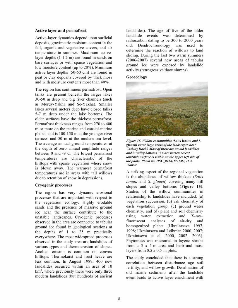
Figure 13. Vaskiny Dachi-2 study site on Terrace III. The soils are a mix of sand and clay. The vegetation is heterogeneous, but dominated by Betula nana, Calamagrostis holmii, Carex bigelowii, Vaccinium vitis-idaea, Aulacomnium turgidum, Hylocomium splendens, and Ptilidium ciliare. Photo DSC_0344, 8/25/07, P. Kuss. ...............................................................7
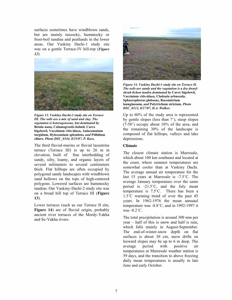
Figure 14. Vaskiny Dachi-3 study site on Terrace II. The soils are sandy and the vegetation is a dry dwarf-shrub-lichen tundra dominated by Carex bigelowii, Vaccinium vitis-idaea, Cladonia arbuscula, Sphaerophorus globosus, Racomitrium lanuginosum, and Polytrichum strictum. Photo DSC_0112, 8/27/07, D.A. Walker. ....................................................................7
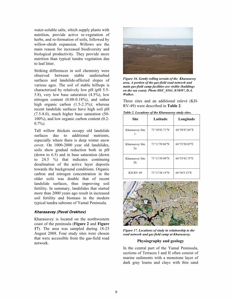
Figure 15. Willow communities (Salix lanata and S. glauca) cover large areas of the landscapes near Vaskiny Dachi. Most of these are on old landslides and in valley bottoms. A more barren recent landslide surface is visible on the upper left side of the photo. Photo no. DSC_0488, 8/21/07, D.A. Walker................................................................................................8
Figure 16. Gently rolling terrain of the Kharasavey area. A portion of the gas-field road network and main gas-field camp facilities are visible (buildings on the sea coast). Photo DSC_0361, 8/30/07, D.A. Walker. ...................................................................................................................9
Figure 17. Locations of study in relationship to the road network and gas field camp at Kharasavey.....................................................................................................................................9
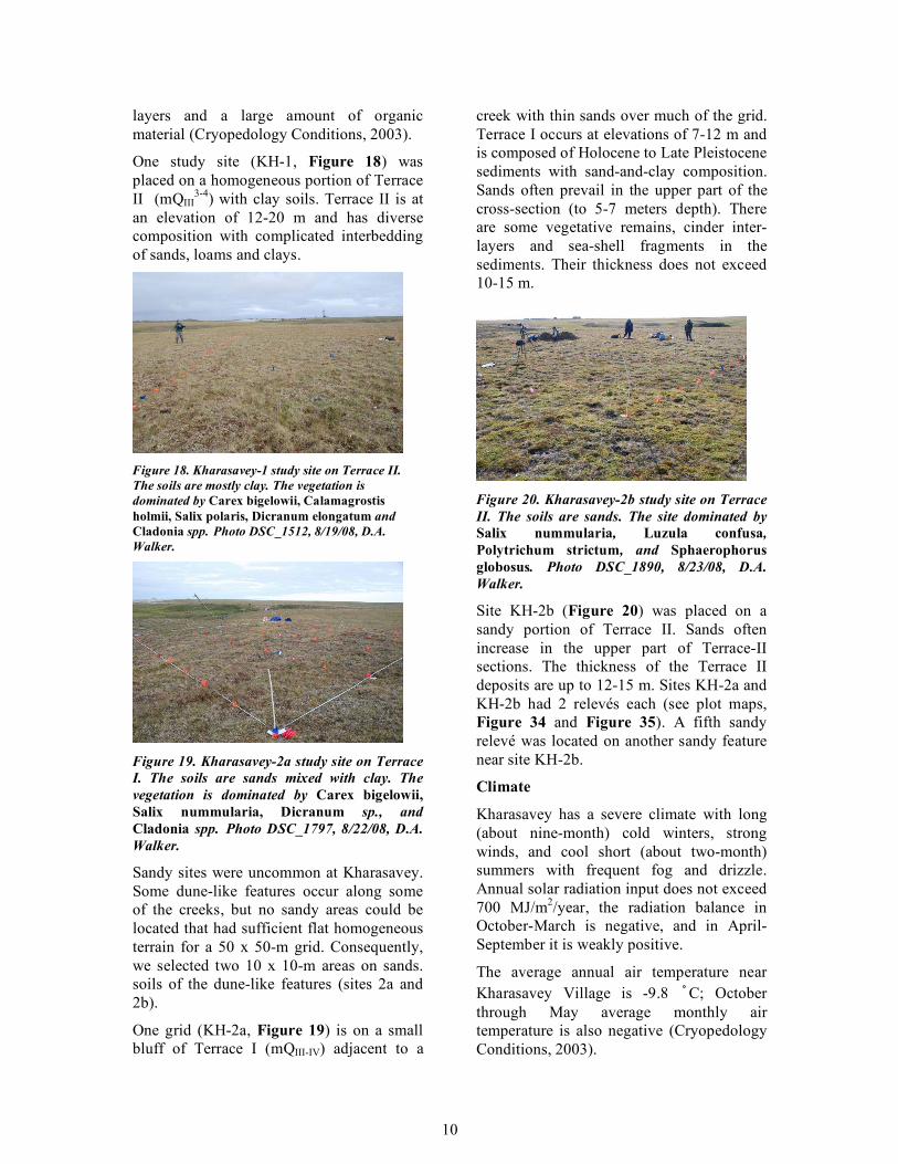
Figure 18. Kharasavey-1 study site on Terrace II. The soils are mostly clay. The vegetation is dominated by Carex bigelowii, Calamagrostis holmii, Salix polaris, Dicranum elongatum and Cladonia spp. Photo DSC_1512, 8/19/08, D.A. Walker. ..................................................10
Figure 19. Kharasavey-2a study site on Terrace I. The soils are sands mixed with clay. The vegetation is dominated by Carex bigelowii, Salix nummularia, Dicranum sp., and Cladonia spp. Photo DSC_1797, 8/22/08, D.A. Walker...........................................................................10
Figure 20. Kharasavey-2b study site on Terrace II. The soils are sands. The site dominated by Salix nummularia, Luzula confusa, Polytrichum strictum, and Sphaerophorus globosus. Photo DSC_1890, 8/23/08, D.A. Walker...................................................................................10
Figure 21. Typical transect and plot layout........................................................................................13 Figure 22. Buckner point-intercept sampling device. The box on the end piece of the device
contains a mirror that can be pointed down to the ground or up to the forest canopy. The tube is a telescope that magnifies the image in the mirror. Cross hairs in the sighting device identify a point that intercepts a plant species which is recorded as a “hit”. The percentage cover of an individual species or cover type is the number of hits for that type divided by the total number of hits. Photo no. DSC_0151, 8/06/07, D.A. Walker. .........................................14
Figure 23. Howie Epstein sampling NDVI using the PSII Spectrometer. Photo no. DSC_0175, 8/23/07, D.A. Walker. .................................................................................................................14
Figure 24. Anatoly Gubarkov with active-layer probe used for measuring depth to the permafrost table. Photo no. DSC_0180, 8/27/07, D.A. Walker. .................................................................15
Figure 25. An iButton logger wrapped in duct tape with the logger number. .................................16 Figure 26. Map of transects and vegetation study plots at Nadym-1. ..............................................19 Figure 27. Map of transects and vegetation study plots at Nadym-2. ..............................................19
vi
Figure 28. Map of transects and vegetation study plots at Laborovaya-1........................................19 Figure 29. Map of transects and vegetation study plots at Laborovaya-2........................................19 Figure 30. Map of transects and vegetation study plots at Vaskiny Dachi-1...................................20 Figure 31. Map of transects and vegetation study plots at Vaskiny Dachi-2...................................20 Figure 32. Map of transects and vegetation study plots at Vaskiny Dachi-3...................................20 Figure 33. Map of transects and vegetation study plots at Kharasavey-1. .......................................21 Figure 34. Map of transects and vegetation study plots at Kharasavey-2a. .....................................21 Figure 35. Map of transects and vegetation study plots at Kharasavey-2b. .....................................21 Figure 36. Mean leaf-area index of transects. ....................................................................................33 Figure 37. LAI vs. overstory biomass for all sites. ............................................................................33 Figure 38. Mean NDVI of sample transects.......................................................................................33 Figure 39. NDVI vs. LAI for all transects..........................................................................................34 Figure 40. NDVI vs biomass for all sites. ..........................................................................................34 Figure 41. Total live and dead biomass including trees. ..................................................................56 Figure 42. Total live biomass..............................................................................................................57 Figure 43. Total biomass excluding trees...........................................................................................58 Figure 44. Total live biomass excluding trees. ..................................................................................59 Figure 45. (a) Soil pit at Nadym – 1 (pit №1), higher microsite. (b) Close up of pit wall..............60 Figure 46. (a) Soil pit at Nadym – 1 (pit №2), lower microsite. (b) Close up of pit wall. ..............61 Figure 47. (a) Soil pit at Nadym - 2 (pit №3), higher hummock microsite. (b) Close up of pit wall.
......................................................................................................................................................62 Figure 48. (a) Soil pit at Nadym – 2 (pit №4), lower inter-hummock microsite. ............................63 Figure 49. (a) Soil pit at Laborovaya-1 (pit №5). (b) Close up of pit wall. .....................................64 Figure 50. (a) Soil pit at Laborovaya-2 (pit №6), higher polygon microsite. (b) Close up of pit
wall. ..............................................................................................................................................65 Figure 51. (a) Close up of soil pit wall at Laborovaya-2b (pit №7). ................................................66 Figure 52. (a) Soil pit at Vaskiny Dachi-1 (pit №8), higher microsite. (b) Close up of pit wall. ...67 Figure 53. (a) Soil pit at Vaskiny Dachi-1 (pit №9), lower microsite. (b) Close up of pit wall. ....68 Figure 54. (a) Soil pit at Vaskiny Dachi-2 (pit №10), lower microsite. (b) Close up of pit wall. ..69 Figure 55. (a) Soil pit at Vaskiny Dachi-2 (pit №11), higher microsite. (b) Close up of pit wall. .70 Figure 56. (a) Soil pit at Vaskiny Dachi-3 (pit №12). (b) Closeup of pit wall. ..............................71 Figure 57. (a) Soil pit at Vaskiny Dachi-3 (pit № 13), inter-polygon lower microsite. (b) Close up
of pit wall. ....................................................................................................................................72 Figure 58. Soil pit at Kharasavey – 1 (р. №1-08) ..............................................................................74 Figure 59. Soil pit at Kharasavey – 2a (р. №2-08) ............................................................................75 Figure 60. Soil pit at Kharasavey – 2b (р. №3-08)............................................................................76
vii
Figure C - 1. Site Description Codes ..................................................................................................86 Figure F - 1. Soils – Nadym 1 .......................................................................................................... 101 Figure F - 2. Soils - Nadym 2........................................................................................................... 102 Figure F - 3. Soils - Laborovaya 1 .................................................................................................. 103 Figure F - 4. Soils - Laborovaya 2 ................................................................................................... 104 Figure F - 5. Soils - Vaskiny Dachi 1 .............................................................................................. 105 Figure F - 6. Soils - Vaskiny Dachi 2 .............................................................................................. 106 Figure F - 7. Soils - Vaskiny Dachi 3 .............................................................................................. 107 Figure F - 8. Soils — Kharasavey 1................................................................................................. 108 Figure F - 9. Soils — Kharasavey-2a, -2b, and RV-49 .................................................................. 109 Figure F - 10. Vegetation – Nadym 1 .............................................................................................. 110 Figure F - 11. Vegetation - Nadym 2............................................................................................... 111 Figure F - 12. Vegetation – Laborovaya 1 ...................................................................................... 113 Figure F - 13. Vegetation – Laborovaya 2 ...................................................................................... 114 Figure F - 14. Vegetation – Vaskiny Dachi 1 ................................................................................. 115 Figure F - 15. Vegetation - Vaskiny Dachi 2 .................................................................................. 116 Figure F - 16. Vegetation - Vaskiny Dachi 3 .................................................................................. 117 Figure F - 17. Vegetation – Kharasavey 1....................................................................................... 118 Figure F - 18. Kharasavey-1 (cont’) ................................................................................................ 119 Figure F - 19. Kharasavey-2a ........................................................................................................... 120 Figure F - 20. Kharasavey-2b........................................................................................................... 121
viii
LIST OF TABLES Table 1. Climate conditions of the Nadym site. ....………………………………………………3 Table 2. Locations of the Kharasavey study sites................................................................................9 Table 3. Study locations, site numbers, site names, and geological settings. ..................................13 Table 4. Dominant vegetation at each study site. ..............................................................................13 Table 5. Logger numbers (on outside of duct tape) and iButton serial numbers.............................16 Table 6. Locations of iButton loggers in relevés and depths. ...........................................................17 Table 7. GPS coordinates and elevations of vegetation study plots and transects. LA =
Laborovaya, ND = Nadym, VD = Vaskiny Dachi. RV = Relevé, T = Transect. Coordinates are recorded at the southwest corner of each grid, and at both ends of the transects (00 and 50 m).............................................................................................................................................22
Table 8. Nadym-1 (forest site) cover along transects. 6 Aug 2007. Skip Walker, Elena Kaerkjärvi, Natalya Moskalenko, Pinus Sylvestris-Cladina stellaris forest. Five 100-m transects, observations at 1-m intervals. Record top species in tree layer, shrub layer, and moss layer at each point. 505 total points. ........................................................................................................23
Table 9. Nadym-2 (CALM-grid site) cover along transect. “Overstory” species are those recorded at the top of the plant canopy at each point; “understory” species are those recorded at the base of the plant canopy; (l) - live green plant part, (d) – dead or senescent plant part. Species use six letter abbreviations. Only two transects were sampled at Nadym-2 because of the limited area available for sampling. Sample points were identified as one of three microsites: hummocks, inter-hummocks, and wet inter-hummocks. .......................................24
Table 10. Laborovaya-1 (clayey site) cover along transects. “Overstory” species are those recorded at the top of the plant canopy at each point; “understory” species are those recorded at the base of the plant canopy. Species use six letter abbreviations, sometimes followed by L (live green plant part) or D (dead or senescent plant part). ...................................................25
Table 11. Laborovaya-2 (sandy site) cover along transects. “Overstory” species are those recorded at the top of the plant canopy at each point; understory” species are those recorded at the base of the plant canopy. Species use six letter abbreviations, sometimes followed by L (live green plant part) or D (dead or senescent plant part). ...................................................26
Table 12. Vaskiny Dachi-1 (Terrace-IV) cover along transects. “Overstory” species are those recorded at the top of the plant canopy at each point; “understory” species are those recorded at the base of the plant canopy. Species use six letter abbreviations, sometimes followed by L (live green plant part) or D (dead or senescent plant part). ...................................................27
Table 13. Vaskiny Dachi-2 (Terrace-III) cover along transects. “Overstory” species are those recorded at the top of the plant canopy at each point; “understory” species are those recorded at the base of the plant canopy. L - live green plant part; D – dead or senescent plant part. Species use six letter abbreviations. ...........................................................................................28
Table 14. Vaskiny Dachi-3 (Terrace-II) cover along transects.........................................................30 Table 15. Kharasavey-1 (Clayey) cover along transects. “Overstory” species are those recorded at
the top of the plant canopy at each point; “understory” species are those recorded at the base of the plant canopy. Species use six letter abbreviations, sometimes followed by L (live green plant part) or D (dead or senescent plant part). ...............................................................31

ix
Table 16. Kharasavey-2a (Sandy) cover along transects. “Overstory” species are those recorded at the top of the plant canopy at each point; “understory” species are those recorded at the base of the plant canopy. Species use six letter abbreviations, sometimes followed by L (live green plant part) or D (dead or senescent plant part). ...............................................................32
Table 17. Kharasavey-2b (Sandy) cover along transects. “Overstory” species are those recorded at the top of the plant canopy at each point; “understory” species are those recorded at the base of the plant canopy. Species use six letter abbreviations, sometimes followed by L (live green plant part) or D (dead or senescent plant part) ................................................................32
Table 18. Point-centered quarter data for Nadym-1 with species arranged alphabetically within each transect. 10 points (40 trees) were sampled along each transect (200 trees total). Abbreviations: Betpub= Betula pubescens, Larsib=Larix sibirica, Pinsib=Pinus cembra ssp. sibirica Pinsyl=Pinus sylvestris. (See Appendix B for explanation of method and data sheets). ..........................................................................................................................................35
Table 19. Summary of point-centered quarter data: Density, basal area, height, and biomass for each tree species and all tree species for each transect and average for all transects. ............36
Table 20. Active layer at Laborovaya and Vaskiny Dachi transects and relevés. Depths are in centimeters. ..................................................................................................................................37
Table 21. Relevé descriptions. Characteristic species use six letter abbreviations (first three letters of genus name + first three letters of species name). Observers: PK, Patrick Kuss; NM, Nataliya Moskalenko; EK, Elina Kärlajaarvi, SW, Skip Walker. Photo archives are at UAF.......................................................................................................................................................38
Table 22. Relevé site characteristics. See data forms (Appendix C). ...............................................39 Table 23. Relevé Soils Data for relevés 1-49.....................................................................................41 Table 24. Species percentage cover in vegetation study plots (relevés). Nomenclature for vascular
plants followed Elven et al. 2007: Checklist of the Panarctic Flora (PAF). Vascular plants. -Draft. University of Oslo. Nomenclature for lichens followed H. Kristinsson & M. Zhurbenko 2006: Panarctic lichen checklist (http://archive.arcticportal.org/276/01/Panarctic_lichen_checklist.pdf). Nomenclature for mosses followed M.S. Ignatov, O.M. Afonina & E.A. Ignatova 2006: Check-list of mosses of East Europe and North Asia. Arctoa 15: 1-130 and for liverworts N.A. Konstantinova & A.D. Potemkin 1996: Liverworts of Russian Arctic: an annotated check-list and bibliography. Arctoa 6: 125-150. ...............................................................................................42
Table 25. Raw plot-count data from the Nadym-1 relevés. All trees in each 10 x 10-m plot were recorded, including diameter at breast height (dbh), basal area of the stem at breast height, height of the tree, and above-ground mass of the tree. Mass was determined using the equations presented in the methods (from Zianis et al. 2005). The location of the tree is given by the x and y coordinates measured in meters from the southwest corner of the plot.......................................................................................................................................................50
Table 26. Summary of tree data from the plot-count method (biomass, basal area, density, and tree height) at Nadym-1...............................................................................................................51
Table 27. Summary of number of trees and seedlings from each relevé at Nadym-1.....................52 Table 28. Comparison of tree biomass as determined by the plot-count method and the point-
centered quarter method. .............................................................................................................53 Table 29. Summary of above-ground plant biomass for the vegetation study plots (relevés). Tree
biomass for each plot was determined from the plot-count method. See Appendix D for
x
biomass sampling and sorting methods for the non-tree species. For the trees, biomass was determined from the plot-count method and expressed in g m-2. .............................................54
Table 30. Biomass data for Figure 41 summarized by site (T = Trace amounts). ...........................56 Table 31. Biomass data for Figure 42 summarized by site ...............................................................57 Table 32. Biomass data for Figure 43 summarized by site. ..............................................................58 Table 33 Biomass data for Figure 44 summarized by site ................................................................59 Table 34. Summary of mean chemical properties for the Nadym-2 Histoturbels. Smallest N for
any variable is 66. ........................................................................................................................73
Table B - 1. Data form for sampling species cover along transects using the Buckner Sample ....84
Table C - 1.Relevé data form: Site description, and growth form cover valuesError! Bookmark
not defined. Table C - 2. Species cover/abundance ................................................................................................87
Table D - 1. Form for above ground biomass sorting........................................................................94 Table D - 2. Aboveground biomass weights ......................................................................................95
Table E - 1. Field Data Sheets:............................................................................................................96 Table E - 2. Summary data sheet, Transect No..................................................................................97
1
INTRODUCTION AND BACKGROUND
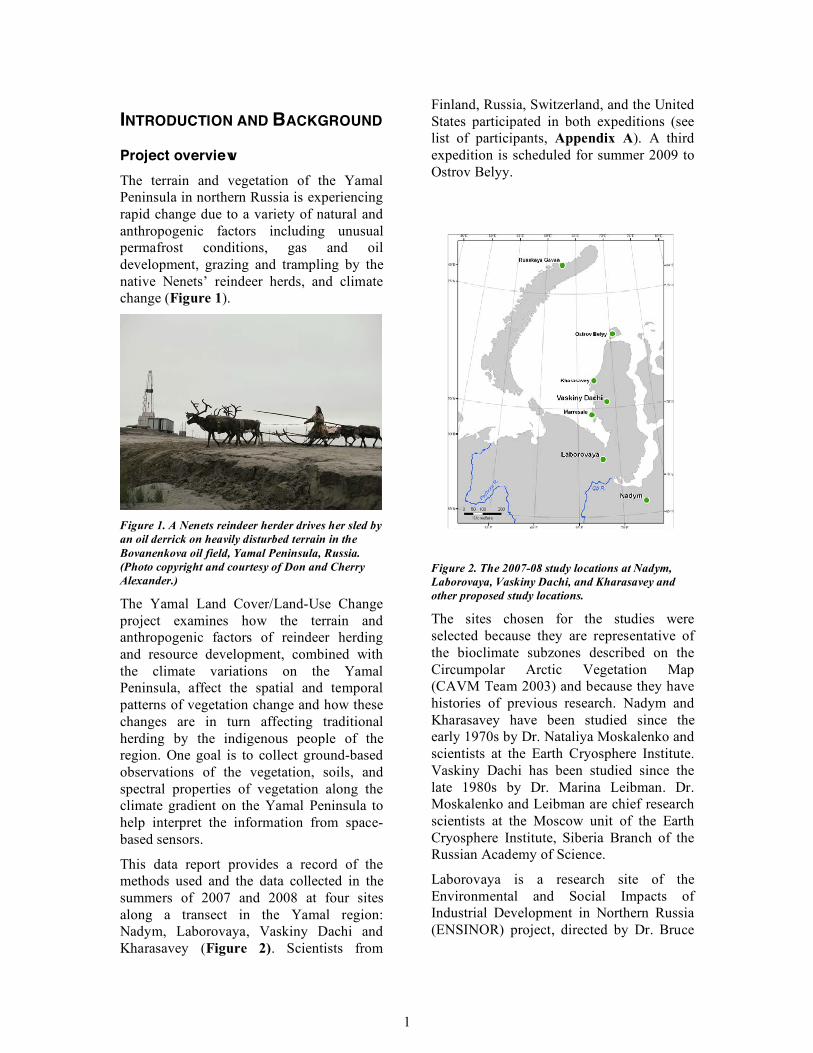
Project overview The terrain and vegetation of the Yamal Peninsula in northern Russia is experiencing rapid change due to a variety of natural and anthropogenic factors including unusual permafrost conditions, gas and oil development, grazing and trampling by the native Nenets’ reindeer herds, and climate change (Figure 1).
Figure 1. A Nenets reindeer herder drives her sled by an oil derrick on heavily disturbed terrain in the Bovanenkova oil field, Yamal Peninsula, Russia. (Photo copyright and courtesy of Don and Cherry Alexander.)
The Yamal Land Cover/Land-Use Change project examines how the terrain and anthropogenic factors of reindeer herding and resource development, combined with the climate variations on the Yamal Peninsula, affect the spatial and temporal patterns of vegetation change and how these changes are in turn affecting traditional herding by the indigenous people of the region. One goal is to collect ground-based observations of the vegetation, soils, and spectral properties of vegetation along the climate gradient on the Yamal Peninsula to help interpret the information from space-based sensors.
This data report provides a record of the methods used and the data collected in the summers of 2007 and 2008 at four sites along a transect in the Yamal region: Nadym, Laborovaya, Vaskiny Dachi and Kharasavey (Figure 2). Scientists from
Finland, Russia, Switzerland, and the United States participated in both expeditions (see list of participants, Appendix A). A third expedition is scheduled for summer 2009 to Ostrov Belyy.
Figure 2. The 2007-08 study locations at Nadym, Laborovaya, Vaskiny Dachi, and Kharasavey and other proposed study locations.
The sites chosen for the studies were selected because they are representative of the bioclimate subzones described on the Circumpolar Arctic Vegetation Map (CAVM Team 2003) and because they have histories of previous research. Nadym and Kharasavey have been studied since the early 1970s by Dr. Nataliya Moskalenko and scientists at the Earth Cryosphere Institute. Vaskiny Dachi has been studied since the late 1980s by Dr. Marina Leibman. Dr. Moskalenko and Leibman are chief research scientists at the Moscow unit of the Earth Cryosphere Institute, Siberia Branch of the Russian Academy of Science.
Laborovaya is a research site of the Environmental and Social Impacts of Industrial Development in Northern Russia (ENSINOR) project, directed by Dr. Bruce
2
Forbes of the Arctic Centre, University of Lapland, Rovaniemi, Finland.
Description of the study sites
Nadym (Nataliya Moskalenko)
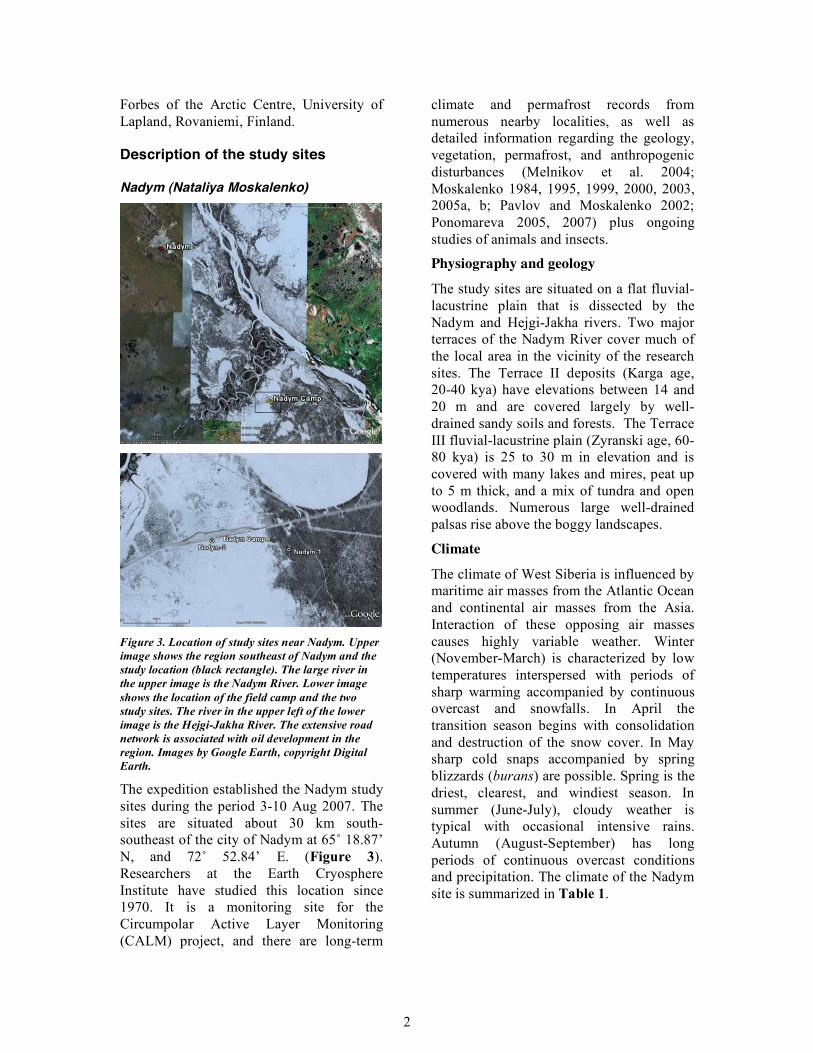
Figure 3. Location of study sites near Nadym. Upper image shows the region southeast of Nadym and the study location (black rectangle). The large river in the upper image is the Nadym River. Lower image shows the location of the field camp and the two study sites. The river in the upper left of the lower image is the Hejgi-Jakha River. The extensive road network is associated with oil development in the region. Images by Google Earth, copyright Digital Earth.
The expedition established the Nadym study sites during the period 3-10 Aug 2007. The sites are situated about 30 km south-southeast of the city of Nadym at 65˚ 18.87’ N, and 72˚ 52.84’ E. (Figure 3). Researchers at the Earth Cryosphere Institute have studied this location since 1970. It is a monitoring site for the Circumpolar Active Layer Monitoring (CALM) project, and there are long-term
climate and permafrost records from numerous nearby localities, as well as detailed information regarding the geology, vegetation, permafrost, and anthropogenic disturbances (Melnikov et al. 2004; Moskalenko 1984, 1995, 1999, 2000, 2003, 2005a, b; Pavlov and Moskalenko 2002; Ponomareva 2005, 2007) plus ongoing studies of animals and insects.
Physiography and geology
The study sites are situated on a flat fluvial-lacustrine plain that is dissected by the Nadym and Hejgi-Jakha rivers. Two major terraces of the Nadym River cover much of the local area in the vicinity of the research sites. The Terrace II deposits (Karga age, 20-40 kya) have elevations between 14 and 20 m and are covered largely by well-drained sandy soils and forests. The Terrace III fluvial-lacustrine plain (Zyranski age, 60-80 kya) is 25 to 30 m in elevation and is covered with many lakes and mires, peat up to 5 m thick, and a mix of tundra and open woodlands. Numerous large well-drained palsas rise above the boggy landscapes.
Climate
The climate of West Siberia is influenced by maritime air masses from the Atlantic Ocean and continental air masses from the Asia. Interaction of these opposing air masses causes highly variable weather. Winter (November-March) is characterized by low temperatures interspersed with periods of sharp warming accompanied by continuous overcast and snowfalls. In April the transition season begins with consolidation and destruction of the snow cover. In May sharp cold snaps accompanied by spring blizzards (burans) are possible. Spring is the driest, clearest, and windiest season. In summer (June-July), cloudy weather is typical with occasional intensive rains. Autumn (August-September) has long periods of continuous overcast conditions and precipitation. The climate of the Nadym site is summarized in Table 1.

3
Table 1. Climate conditions of the Nadym site.
Average air temperature (°C): Annual -5.9 Summer 10.8 Winter -14.2 Annual amplitude (meteorological), °C 40.5 Mean-annual ground-surface temp. (°C) +1 to -3 Date of transition of air temp through 0 °C In the spring 27 May In the autumn 20 Oct Precipitation (mm): Annual 483 Liquid 237 Snow cover: Date of formation 15 Oct Date of melting 27 May Maximum depth (April) (cm) 76 Average density (in April), kg m-3 290
Soils
The Nadym research sites are situated in the northern taiga bioclimate subzone. A wide variety of ecosystems are present due to Nadym’s position within this transitional region. The parent materials for the soils are derived from fluvial-lacustrine deposits. Mainly sandy materials interbedded with loamy and clay deposits were repeatedly spread by the river systems. The heterogeneous soil textures complicate the permafrost distribution patterns. Key soil processes are peat accumulation, gleying and podzolization. In well-drained forested ecosystems on Terrace II, podzolic soils are common with evidence of previous cryogenic attributes, such as networks of former ice wedges (pseudomorphs) that are filled with loamy and/or clayey materials. On Terrace III, superimposed on these sandy soils, are the effects of various bog-forming and metamorphic cryogenic processes (including paludification, thermokarst, frost heave, and thermal abrasion) that create a heterogeneous complex of soils with permafrost landforms and peatlands with peat-gley soils.
Vegetation
Figure 4. Nadym-1 (forest site). The trees are mainly Scots pine (Pinus sylvestris), and mountain birch (Betula tortuosa) mixed with Siberian larch (Larix sibirica). The understory consists of dwarf shrubs (Ledum palustre, Betula nana, Empetrum nigrum, Vaccinium uliginosum, V. vitis-idaea), lichens (mainly Cladonia stellaris) and mosses (mainly Pleurozium schreberi). Photo no. DSC_0325, 8/09/07, P. Kuss.
Figure 5. Nadym-2 (CALM-grid site). Hummocky tundra consists of a complex of vegetation with a Ledum palustre-Betula nana-Cladonia spp. dwarf-shrub community on the hummocks and a Cladonia stellaris-Carex glomerata lichen community in the inter-hummock areas. Photo no. DSC_0101 8/03/07, D.A. Walker.
Zonal northern taiga forest covers large areas of Terrace II. Here there are birch-larch (Betula tortuosa-Larix sibirica) and birch-pine shrub-lichen (Betula tortuosa-Pinus sylvestris/Betula nana-Cladonia stellaris) open woodlands.
Terrace III is characterized by peatlands occupied by Rubus chamaemorus-Ledum palustre-Sphagnum-lichen tundra on raised palsas and elevated microsites and Eriophorum-Carex-Sphagnum mires in the lower microsites. Large frost mounds also occur in these peatlands and are
4
characterized by Pinus sibirica-Ledum palustre-Cladonia open woodlands.
Our Nadym-1 study site (forest site) is located in a lichen woodland on Terrace II (Figure 4), and the Nadym-2 study site (CALM Grid site) is located on Terrace III at the 100 x 100-m CALM grid in hummocky tundra (Figure 5). The study areas are currently not used by the Nenets for reindeer forage lands, so the lichen areas are well preserved at both sites.
Laborovaya (Bruce Forbes)
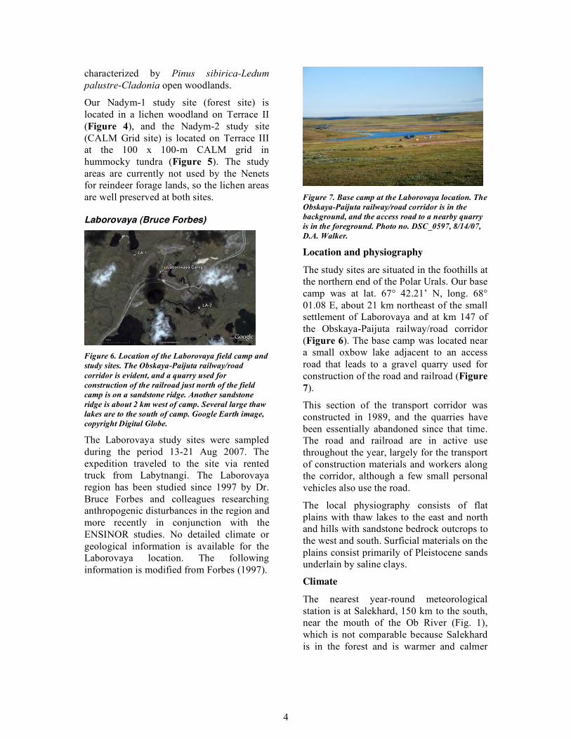
Figure 6. Location of the Laborovaya field camp and study sites. The Obskaya-Paijuta railway/road corridor is evident, and a quarry used for construction of the railroad just north of the field camp is on a sandstone ridge. Another sandstone ridge is about 2 km west of camp. Several large thaw lakes are to the south of camp. Google Earth image, copyright Digital Globe.
The Laborovaya study sites were sampled during the period 13-21 Aug 2007. The expedition traveled to the site via rented truck from Labytnangi. The Laborovaya region has been studied since 1997 by Dr. Bruce Forbes and colleagues researching anthropogenic disturbances in the region and more recently in conjunction with the ENSINOR studies. No detailed climate or geological information is available for the Laborovaya location. The following information is modified from Forbes (1997).
Figure 7. Base camp at the Laborovaya location. The Obskaya-Paijuta railway/road corridor is in the background, and the access road to a nearby quarry is in the foreground. Photo no. DSC_0597, 8/14/07, D.A. Walker.
Location and physiography
The study sites are situated in the foothills at the northern end of the Polar Urals. Our base camp was at lat. 67° 42.21’ N, long. 68° 01.08 E, about 21 km northeast of the small settlement of Laborovaya and at km 147 of the Obskaya-Paijuta railway/road corridor (Figure 6). The base camp was located near a small oxbow lake adjacent to an access road that leads to a gravel quarry used for construction of the road and railroad (Figure 7).
This section of the transport corridor was constructed in 1989, and the quarries have been essentially abandoned since that time. The road and railroad are in active use throughout the year, largely for the transport of construction materials and workers along the corridor, although a few small personal vehicles also use the road.
The local physiography consists of flat plains with thaw lakes to the east and north and hills with sandstone bedrock outcrops to the west and south. Surficial materials on the plains consist primarily of Pleistocene sands underlain by saline clays.
Climate
The nearest year-round meteorological station is at Salekhard, 150 km to the south, near the mouth of the Ob River (Fig. 1), which is not comparable because Salekhard is in the forest and is warmer and calmer
5
than the Laborovaya region. Laborovaya lies within the continuous permafrost zone.
Vegetation
Phytogeographically, the study site lies about 100 km north of the latitudinal treeline within the southern tundra subzone (= Subzone E of the Circumpolar Arctic Vegetation Map, (CAVM Team et al. 2003)). According to Yurtsev (1994), the Yamal-Gydan West Siberian subprovince is characterized by a low floristic richness due to gaps in the ranges of species with predominantly montane, east Siberian distributions and western (amphi-Atlantic) distributions. The region's vegetation has been mapped at small scale (Ilyina et al., 1976) and its community types described by Meltzer (1984).
Ridge tops on the sandstone hills are dry. Well-developed stands of alder (Alnus fruticosa) are common on slopes in the vicinity of the study site and especially in riparian zones. Shrub willows (Salix spp.) are generally <30 cm in height, although individuals >2 m occur in riparian zones and on hillslopes. The areas between hills are a mix of wetlands and more mesic vegetation. Much of the tundra is overgrazed with only sparse lichen cover. The study area is extensively grazed in summer by reindeer herds belonging to the Nenets, a group of aboriginal nomadic pastoralists. Vilchek & Bykova (1992) estimated that the number of reindeer on Yamal is already 1.5 to 2 times greater than the optimum for the region.
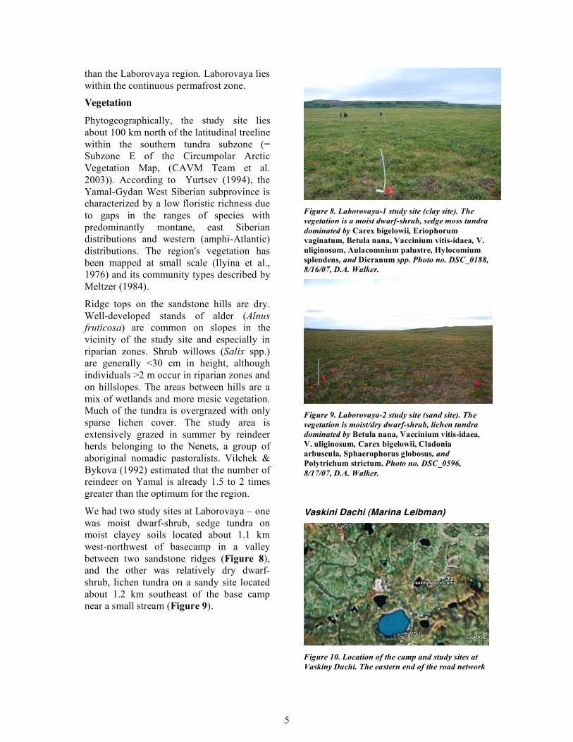
We had two study sites at Laborovaya – one was moist dwarf-shrub, sedge tundra on moist clayey soils located about 1.1 km west-northwest of basecamp in a valley between two sandstone ridges (Figure 8), and the other was relatively dry dwarf-shrub, lichen tundra on a sandy site located about 1.2 km southeast of the base camp near a small stream (Figure 9).
Figure 8. Laborovaya-1 study site (clay site). The vegetation is a moist dwarf-shrub, sedge moss tundra dominated by Carex bigelowii, Eriophorum vaginatum, Betula nana, Vaccinium vitis-idaea, V. uliginosum, Aulacomnium palustre, Hylocomium splendens, and Dicranum spp. Photo no. DSC_0188, 8/16/07, D.A. Walker.
Figure 9. Laborovaya-2 study site (sand site). The vegetation is moist/dry dwarf-shrub, lichen tundra dominated by Betula nana, Vaccinium vitis-idaea, V. uliginosum, Carex bigelowii, Cladonia arbuscula, Sphaerophorus globosus, and Polytrichum strictum. Photo no. DSC_0596, 8/17/07, D.A. Walker.
Vaskini Dachi (Marina Leibman)
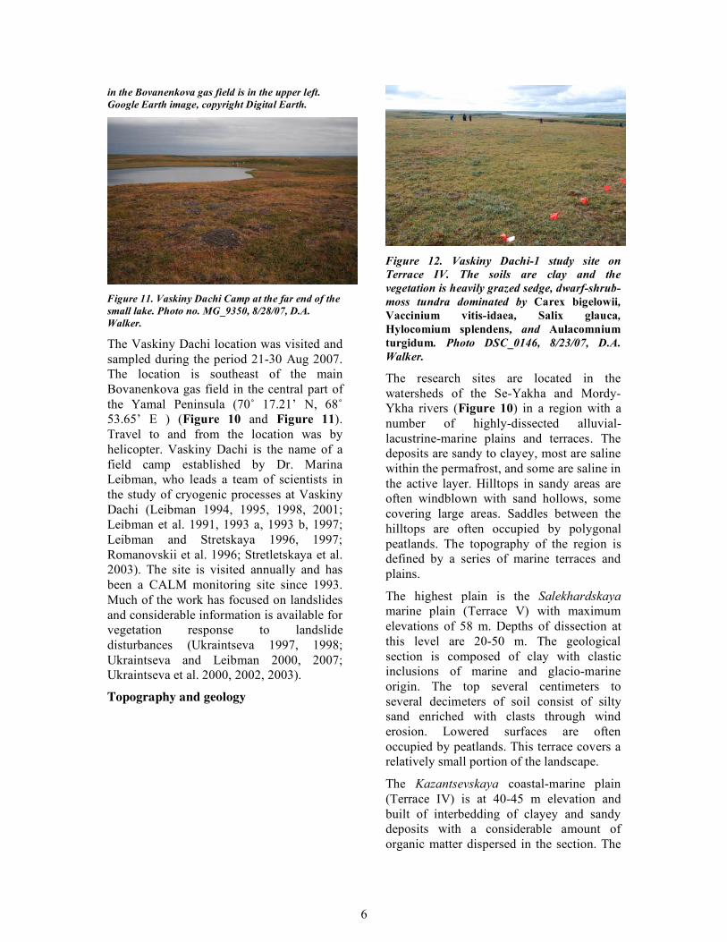
Figure 10. Location of the camp and study sites at Vaskiny Dachi. The eastern end of the road network
6
in the Bovanenkova gas field is in the upper left. Google Earth image, copyright Digital Earth.
Figure 11. Vaskiny Dachi Camp at the far end of the small lake. Photo no. MG_9350, 8/28/07, D.A. Walker.
The Vaskiny Dachi location was visited and sampled during the period 21-30 Aug 2007. The location is southeast of the main Bovanenkova gas field in the central part of the Yamal Peninsula (70˚ 17.21’ N, 68˚ 53.65’ E ) (Figure 10 and Figure 11). Travel to and from the location was by helicopter. Vaskiny Dachi is the name of a field camp established by Dr. Marina Leibman, who leads a team of scientists in the study of cryogenic processes at Vaskiny Dachi (Leibman 1994, 1995, 1998, 2001; Leibman et al. 1991, 1993 a, 1993 b, 1997; Leibman and Stretskaya 1996, 1997; Romanovskii et al. 1996; Stretletskaya et al. 2003). The site is visited annually and has been a CALM monitoring site since 1993. Much of the work has focused on landslides and considerable information is available for vegetation response to landslide disturbances (Ukraintseva 1997, 1998; Ukraintseva and Leibman 2000, 2007; Ukraintseva et al. 2000, 2002, 2003).
Topography and geology
Figure 12. Vaskiny Dachi-1 study site on Terrace IV. The soils are clay and the vegetation is heavily grazed sedge, dwarf-shrub-moss tundra dominated by Carex bigelowii, Vaccinium vitis-idaea, Salix glauca, Hylocomium splendens, and Aulacomnium turgidum. Photo DSC_0146, 8/23/07, D.A. Walker.
The research sites are located in the watersheds of the Se-Yakha and Mordy-Ykha rivers (Figure 10) in a region with a number of highly-dissected alluvial-lacustrine-marine plains and terraces. The deposits are sandy to clayey, most are saline within the permafrost, and some are saline in the active layer. Hilltops in sandy areas are often windblown with sand hollows, some covering large areas. Saddles between the hilltops are often occupied by polygonal peatlands. The topography of the region is defined by a series of marine terraces and plains.
The highest plain is the Salekhardskaya marine plain (Terrace V) with maximum elevations of 58 m. Depths of dissection at this level are 20-50 m. The geological section is composed of clay with clastic inclusions of marine and glacio-marine origin. The top several centimeters to several decimeters of soil consist of silty sand enriched with clasts through wind erosion. Lowered surfaces are often occupied by peatlands. This terrace covers a relatively small portion of the landscape.
The Kazantsevskaya coastal-marine plain (Terrace IV) is at 40-45 m elevation and built of interbedding of clayey and sandy deposits with a considerable amount of organic matter dispersed in the section. The
7
surfaces sometimes have windblown sands, but are mainly tussocky, hummocky or frost-boil tundras and peatlands in the lower areas. Our Vaskiny Dachi-1 study site was on a gentle Terrace-IV hill-top (Figure 12).
Figure 13. Vaskiny Dachi-2 study site on Terrace III. The soils are a mix of sand and clay. The vegetation is heterogeneous, but dominated by Betula nana, Calamagrostis holmii, Carex bigelowii, Vaccinium vitis-idaea, Aulacomnium turgidum, Hylocomium splendens, and Ptilidium ciliare. Photo DSC_0344, 8/25/07, P. Kuss.
The third fluvial-marine or fluvial lacustrine terrace (Terrace III) is up to 26 m in elevation, built of fine interbedding of sandy, silty, loamy, and organic layers of several milimeters to several centimeters thick. Flat hilltops are often occupied by polygonal sandy landscapes with windblown sand hollows on the tops of high-centered polygons. Lowered surfaces are hummocky tundras. Our Vaskiny-Dachi-2 study site was on a broad hill top of Terrace III (Figure 13).
Lower terraces (such as our Terrace II site, Figure 14) are of fluvial origin, probably ancient river terraces of the Mordy-Yakha and Se-Yakha rivers.
Figure 14. Vaskiny Dachi-3 study site on Terrace II. The soils are sandy and the vegetation is a dry dwarf-shrub-lichen tundra dominated by Carex bigelowii, Vaccinium vitis-idaea, Cladonia arbuscula, Sphaerophorus globosus, Racomitrium lanuginosum, and Polytrichum strictum. Photo DSC_0112, 8/27/07, D.A. Walker.
Up to 60% of the study area is represented by gentle slopes (less than 7˚), steep slopes (7-50˚) occupy about 10% of the area, and the remaining 30% of the landscape is composed of flat hilltops, valleys and lake depressions.
Climate
The closest climate station is Marresale, which about 100 km southeast and located at the coast, where summer temperatures are somewhat cooler than at Vaskiny Dachi. The average annual air temperature for the last 15 years at Marresale is -7.5˚C. The average January temperature over the same period is -21.5˚C, and the July mean temperature is 7.5˚C. There has been a 1.3˚C warming trend of over the past 45 years. In 1962-1976 the mean annuaul temperature was -8.8˚C, and in 1992-1997 it was -8.2˚C.
The total precipitation is around 300 mm per year – half of this is snow and half is rain, which falls mainly in August-September. The end-of-winter-snow depth on flat surfaces is about 30 cm, snow drifts on leeward slopes may be up to 6 m deep. The average period with positive air temperatures at Marresale weather station is 59 days, and the transition to above freezing daily mean temperatures is usually in late June and early October.
8
Active layer and permafrost
Active-layer dynamics depend upon surficial deposits, gravimetric moisture content in the fall, organic and vegetative covers, and air temperature in summer. Maximum active-layer depths (1-1.2 m) are found in sands on bare surfaces or with sparse vegetation and low moisture content (up to 20%). Minimum active layer depths (50-60 cm) are found in peat or clay deposits covered by thick moss and with moisture contents more than 40%.
The region has continuous permafrost. Open taliks are present beneath the larger lakes 30-50 m deep and big river channels (such as Mordy-Yakha and Se-Yakha). Smaller lakes several meters deep have closed taliks 5-7 m deep under the lake bottoms. The older surfaces have the thickest permafrost. Permafrost thickness ranges from 270 to 400 m or more on the marine and coastal-marine plains, and is 100-150 m at the younger river terraces and 50 m at the modern sea level. The average annual ground temperatures at the depth of zero annual amplitude ranges between 0 and -9°C. The lowest permafrost temperatures are characteristic of the hilltops with sparse vegetation where snow is blown away. The warmest permafrost temperatures are in areas with tall willows due to retention of snow in depressions.
Cryogenic processes
The region has very dynamic erosional processes that are important with respect to the vegetation ecology. Highly erodable sands and the presence of massive ground ice near the surface contribute to the unstable landscapes. Cryogenic processes observed in the area are connected to tabular ground ice found in geological sections at the depths of 1 to 25 m practically everywhere. The most widespread processes observed in the study area are landslides of various types and thermoerosion of slopes. Aeolian erosion is common on convex hilltops. Thermokarst and frost heave are less common. In August 1989, 400 new landslides occurred within an area of 10 km2, where previously there were only three modern landslides (but hundreds of ancient
landslides). The age of five of the older landslide events was determined by radiocarbon dating to be 300 to 2000 years old. Dendrochronology was used to determine the reaction of willows to land sliding. During the last two warm summers (2006-2007) several new areas of tabular ground ice were exposed by landslide activity (retrogressive thaw slumps).
Geoecology
Figure 15. Willow communities (Salix lanata and S. glauca) cover large areas of the landscapes near Vaskiny Dachi. Most of these are on old landslides and in valley bottoms. A more barren recent landslide surface is visible on the upper left side of the photo. Photo no. DSC_0488, 8/21/07, D.A. Walker.
A striking aspect of the regional vegetation is the abundance of willow thickets (Salix lanata and S. glauca) covering many hill slopes and valley bottoms (Figure 15). Studies of the willow communities in relationship to landslides have included: (a) vegetation succession, (b) ash chemistry of each vegetation group, (c) ground water chemistry, and (d) plant and soil chemistry using water extraction and X-ray–fluorescent analyses of air-dry and homogenized plants (Ukraintseva 1997, 1998; Ukraintseva and Leibman 2000, 2007; Ukraintseva et al. 2000, 2002, 2003). Phytomass was measured in layers: shrubs from a 5 x 5-m area and herb and moss layers from 0.5 x 0.5-m plots.
The study concluded that there is a strong correlation between disturbance age soil fertility, and willow growth. Desalination of old marine sediments after the landslide event leads to active layer enrichment with
9
water-soluble salts, which supply plants with nutrition, provide active re-vegetation of herbs, and re-formation of soils, followed by willow-shrub expansion. Willows are the main reason for increased biodiversity and biological productivity. They provide more nutrition than typical tundra vegetation due to leaf litter.
Striking differences in soil chemistry were observed between stable undisturbed surfaces and landslide-affected slopes of various ages. The soil of stable hilltops is characterized by relatively low pH (рН 5.5-5.8), very low base saturation (4.5%), low nitrogen content (0.08-0.18%), and rather high organic carbon (1.5-2.3%); whereas recent landslide surfaces have high soil рН (7.5-8.0), much higher base saturation (50-100%), and low organic carbon content (0.2-0.7%).
Tall willow thickets occupy old landslide surfaces due to additional nutrients, especially where there is deep winter snow cover. On 1000-2000 year old landslides, soils show gradual reduction both in рН (down to 6.5) and in base saturation (down to 24.5 %) that indicates continuing desalination of the active layer deposits towards the background conditions. Organic carbon and nitrogen concentration in the older soils was double that of recent landslide surfaces, thus improving soil fertility. In summary, landslides that started more than 2000 years ago result in increased soil fertility and biomass in the modern typical tundra subzone of Yamal Peninsula.
Kharasavey (Pavel Orekhov)
Kharasavey is located on the northwestern coast of the peninsula (Figure 2 and Figure 17). The area was sampled during 18-25 August 2008. Four study sites were chosen that were accessible from the gas-field road network.
Figure 16. Gently rolling terrain of the Kharasavey area. A portion of the gas-field road network and main gas-field camp facilities are visible (buildings on the sea coast). Photo DSC_0361, 8/30/07, D.A. Walker.
Three sites and an additional relevé (KH-RV-49) were described in Table 2. Table 2. Locations of the Kharasavey study sites.
Site Latitude Longitude
Kharasavey Site 1:
71°10'43.71"N 66°58'47.84”E
Kharasavey Site 2a:
71°11'39.86"N 66°53'20.05"E
Kharasavey Site 2b:
71°11'39.98"N 66°55'43.75"E
KH-RV-49 71°11'38.14"N 66°56'5.33"E
Figure 17. Locations of study in relationship to the road network and gas field camp at Kharasavey.
Physiography and geology
In the central part of the Yamal Peninsula, sections of Terraces I and II often consist of marine sediments with a monotone layer of dark gray loams and clays with thin sand
10
layers and a large amount of organic material (Cryopedology Conditions, 2003).
One study site (KH-1, Figure 18) was placed on a homogeneous portion of Terrace II (mQIII
3-4) with clay soils. Terrace II is at an elevation of 12-20 m and has diverse composition with complicated interbedding of sands, loams and clays.
Figure 18. Kharasavey-1 study site on Terrace II. The soils are mostly clay. The vegetation is dominated by Carex bigelowii, Calamagrostis holmii, Salix polaris, Dicranum elongatum and Cladonia spp. Photo DSC_1512, 8/19/08, D.A. Walker.
Figure 19. Kharasavey-2a study site on Terrace I. The soils are sands mixed with clay. The vegetation is dominated by Carex bigelowii, Salix nummularia, Dicranum sp., and Cladonia spp. Photo DSC_1797, 8/22/08, D.A. Walker.
Sandy sites were uncommon at Kharasavey. Some dune-like features occur along some of the creeks, but no sandy areas could be located that had sufficient flat homogeneous terrain for a 50 x 50-m grid. Consequently, we selected two 10 x 10-m areas on sands. soils of the dune-like features (sites 2a and 2b).
One grid (KH-2a, Figure 19) is on a small bluff of Terrace I (mQIII-IV) adjacent to a
creek with thin sands over much of the grid. Terrace I occurs at elevations of 7-12 m and is composed of Holocene to Late Pleistocene sediments with sand-and-clay composition. Sands often prevail in the upper part of the cross-section (to 5-7 meters depth). There are some vegetative remains, cinder inter-layers and sea-shell fragments in the sediments. Their thickness does not exceed 10-15 m.
Figure 20. Kharasavey-2b study site on Terrace II. The soils are sands. The site dominated by Salix nummularia, Luzula confusa, Polytrichum strictum, and Sphaerophorus globosus. Photo DSC_1890, 8/23/08, D.A. Walker.
Site KH-2b (Figure 20) was placed on a sandy portion of Terrace II. Sands often increase in the upper part of Terrace-II sections. The thickness of the Terrace II deposits are up to 12-15 m. Sites KH-2a and KH-2b had 2 relevés each (see plot maps, Figure 34 and Figure 35). A fifth sandy relevé was located on another sandy feature near site KH-2b.
Climate
Kharasavey has a severe climate with long (about nine-month) cold winters, strong winds, and cool short (about two-month) summers with frequent fog and drizzle. Annual solar radiation input does not exceed 700 MJ/m2/year, the radiation balance in October-March is negative, and in April-September it is weakly positive.
The average annual air temperature near Kharasavey Village is -9.8 ˚С; October through May average monthly air temperature is also negative (Cryopedology Conditions, 2003).
11
Monthly mean minimum air temperature is in January and February (-23 and -24 ˚С), while monthly mean maximum temperatures occur in July and August (+6 and +7 ˚С). The absolute minimum air temperature, -49 ˚С, occurred in February, and an absolute maximum of +29 ˚С occurred in July. An average annual sum of monthly positive temperatures is +14.7 ˚С mo and the sum of monthly negative temperatures is -131.3 ˚C mo. Average duration of the frost-free season is 50 days. In spring average daily temperatures usually exceed 0 ˚С at the end of May or at the beginning of June. The first freezing temperatures occur in the third decade of September. In October the season of steady frosts starts (Cryosphere, 2006).
Annual precipitation is 260-300 mm; about half of this falls as snow. The snow cover begins at the end of September or at the beginning of October and melts at the first half of June. The average end-of-winter depth of the snow is 19 cm. Wind redistribution of snow is most active during October-December, when up to 60% of winter precipitation falls. Topographic lows – hollows, ravines and stream valleys –completely fill with snow, and drift depths can reach 4-5 meters. On open and raised areas, snow thickness does not exceed 15-25 cm. In the process of snow accumulation snow density uniformly increases from 0.22 to 0.26 g/cm3 at the beginning of winter to 0.36 g/cm3 by the end of winter.
Landscapes
The landscapes of marine terraces I and II are flat to undulating and covered by tundra mainly with graminoids (sedges, grasses, and rushes), dwarf shrubs, mosses and lichens (Figure 16). The terrace surfaces are relatively well drained and highly dissected by many small gullies and drainages. These drainages are continually expanding and growing through cryogenic landslides and erosion of the underlying massive ground ice. Non-sorted circles are common on many surfaces.
Thermokarst features, such as thaw lakes, drained thaw lakes (khasyreis), small
thermokarst ponds, and ice-wedge polygons, are relatively uncommon within the area of our study (Figure 17), but these features are common in peaty lowlands of the larger streams and rivers in the vicinity of Kharasavey.
Sandy beaches, dunes and coastal bluffs up to 10 m high occur along the seacoast (Cryopedology Conditions, 2003).
Vegetation
The local Kharasavey flora is represented by 27 families, 63 genera and 125 species of vascular plants. The leading families include Poaceae (26 species), Cyperaceae (12 species), Caryophyllaceae (12 species), Brassicaceae (11 species) and Ranunculaceae (9 species) (Rebristaya, 1995).
Common plants on the upland tundra areas include dwarf shrubs (e.g., Salix polaris, Salix lanata, S. glauca), graminoids (e.g, Carex bigelowii, Calamagrostis holmii, Arctagrostis latifolia, Eriophorum angustifolium, Alopecurus alpinus, Poa arctica, Luzula confusa), forbs, (e.g., Saxifraga cernua, S. foliolosa, Rumex arcticus), mosses (e.g., Dicranum elongatum, Polytrichum strictum, Aulacomnium spp., Hylocomium splendens) and lichens (e.g., Cladonia spp., Sphaerophorus globosus, Peltigera aphthosa, Thamnolia subuliformis, and Cetraria spp.).
Well drained creek bluffs and dune like features have tundra dominated by dwarf-shrubs (e.g. Salix nummularia, Vaccinium vitis idaea), graminoids (Luzula confusa, Deschampsia sukatschewii, mosses (e.g., Dicranum elongatum,, and lichens (Avramchik, 1969). Wind eroded areas are common on the sandy features.
At the coast erect willows (osiers) are uncommon and stunted reaching heights of only 15-20 cm; however, several kilometers inland, willows are more abundant and can reach heights of 1-1.5 meters in protected microsites.

12
Wetlands dominated by sedges and mosses cover surfaces with poor drainage conditions. Plants in wet microsites include Carex aquatilis, C. rariflora, Eriophorum angustifolium, Polemonium acutiflorum, Pedicularis sudetica and many moss species (Avramchik 1961c).
The vegetation of the region has been mapped at small scale (1:1,000,000) as part of the Yamalo Nenets Autonomous Area (Avranchik 1961а,b,c, 1969). These maps show the Kharasavey Cape containing sub-Arctic tundras with moss and lichen tundras and Arctic-type wetlands. Highly degraded lichen tundras occur on sandy uplands with polygonal surfaces. All formations are used as a summer and autumn pasture for reindeer.
Literature
Avramchik M.N. (Аврамчик М.Н.) 1969. “The Subzone Characterization of Tundra, Forest-Tundra and Taiga Vegetation in Western Siberian Lowland”. Botanist Journal, №3, vol. 54.
Avramchik M.N. (Аврамчик М.Н.) 1961а. The map of Yamalo Nenets Autonomous Area Vegetation М. 1:1 000 000, 4 pages. 1961 (not published)
Avramchik M.N. (Аврамчик М.Н.) 1961b. “Vegetation of Yamal Nenets Autonomous Area”. The Explanatory Note to Notation Conventions of the Map of Yamalo Nenets Autonomous Area Vegetation at the scale of 1: 1 000 000. 57 pages (not published)
Avramchik M.N. (Аврамчик М.Н.) 1961c. The Explanatory Note to the Key of the Map
of Yamalo Nenets Autonomous Area Vegetation at the scale of 1: 1 000 000. 54 стр. (not published)
Cryopedology Conditions of Harasaway and Krusenstern deposits (Yamal Peninsula) / Baulin V.V. (Баулин В.В.), Dubikov G.I. (Дубиков Г. И .), Aksenov V.I. (Аксенов В. И .) and etc. – М.: GEOS, 2003. – 180 p.
“Cryosphere of Oil and Gas Condensate Fields of Yamal Peninsula: V. 1: Cryosphere of Harasaway Gas Condensate Field”. 2006. 347p. Saint-Petersburg: Nedra, Saint-Petersburg branch, 2006.
Rebristaya O.V. (Ребристая О.В.) 1995. Vascular Plants of Belii Island (Kara Sea)Сосудистые растения острова Белый (Карское море). Botanist Journal. №7, volume 80
METHODS AND TYPES OF DATA COLLECTED Study sites
Criteria for site selection Study sites were selected at each location (Nadym, Laborovaya, Vaskiny Dachi, Kharasavey) in large areas of more or less homogeneous vegetation. The objective was to select large areas of zonal vegetation that could be recognized by their homogeneous spectral signatures on aerial photographs and satellite images. At all three locations there were surfaces with different parent materials that affected the character of the vegetation (Table 3 and Table 4).
13
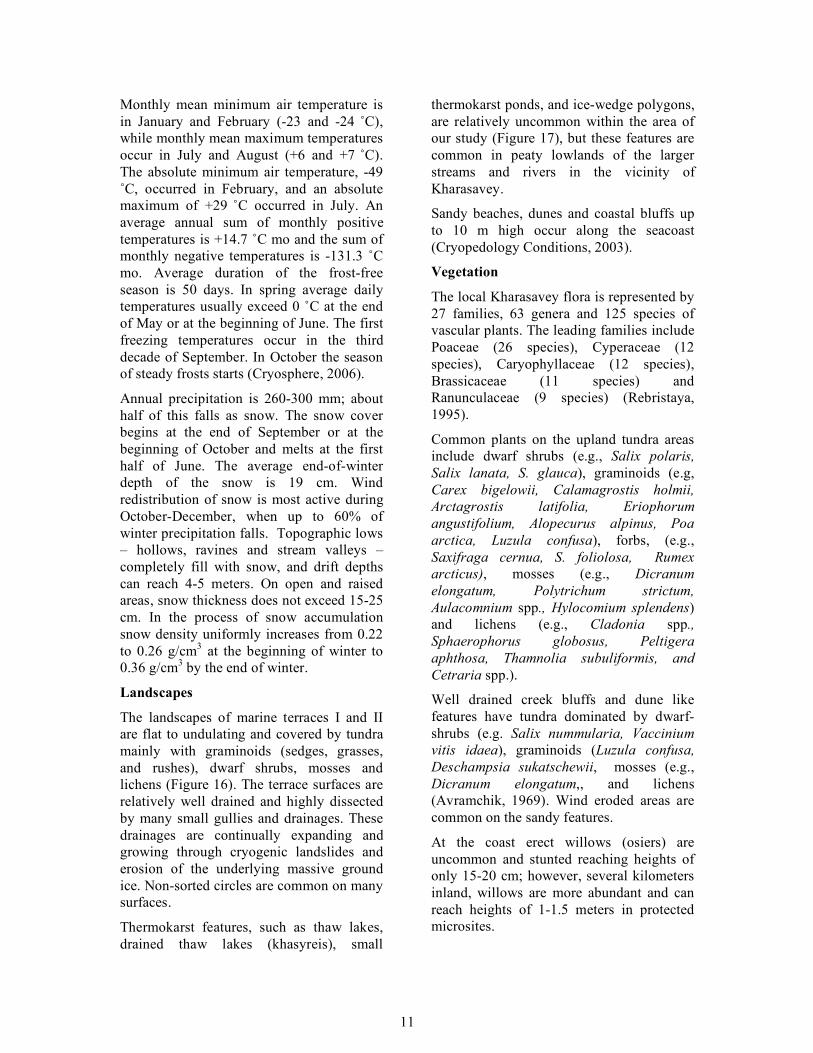
Table 3. Study locations, site numbers, site names, and geological settings.
Table 4. Dominant vegetation at each study site.
Size, arrangement, and marking of transects and study plots
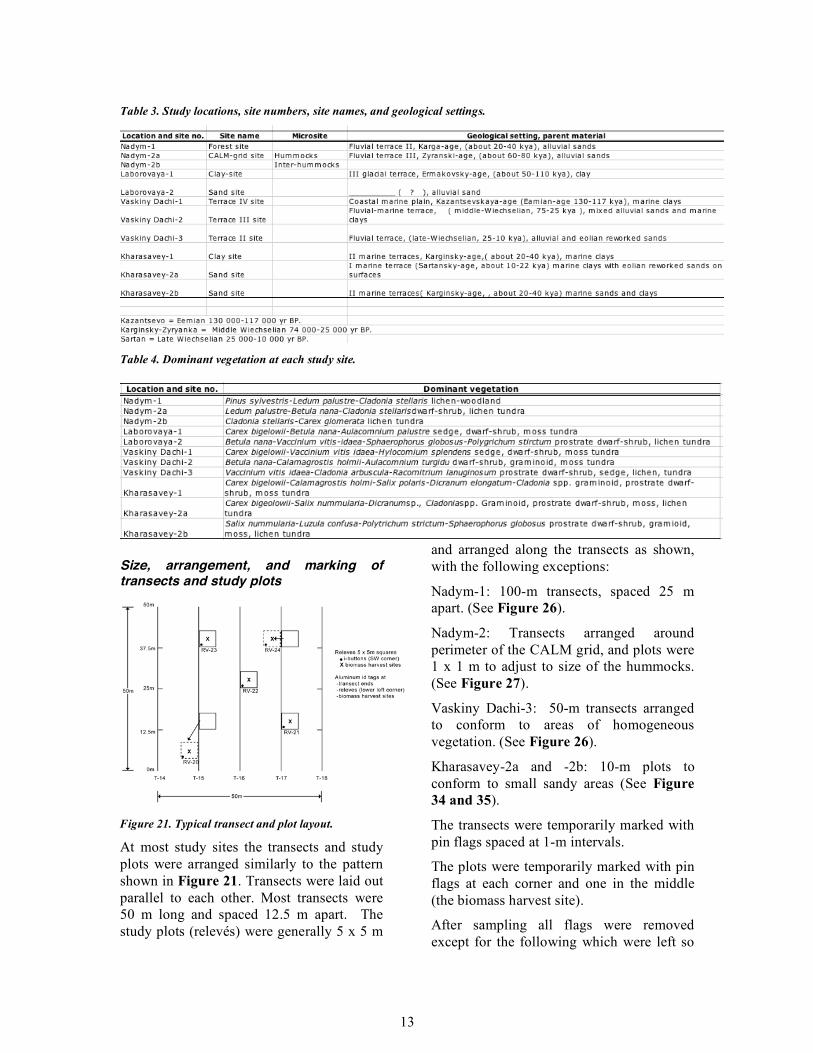
Figure 21. Typical transect and plot layout.
At most study sites the transects and study plots were arranged similarly to the pattern shown in Figure 21. Transects were laid out parallel to each other. Most transects were 50 m long and spaced 12.5 m apart. The study plots (relevés) were generally 5 x 5 m
and arranged along the transects as shown, with the following exceptions:
Nadym-1: 100-m transects, spaced 25 m apart. (See Figure 26).
Nadym-2: Transects arranged around perimeter of the CALM grid, and plots were 1 x 1 m to adjust to size of the hummocks. (See Figure 27).
Vaskiny Dachi-3: 50-m transects arranged to conform to areas of homogeneous vegetation. (See Figure 26).
Kharasavey-2a and -2b: 10-m plots to conform to small sandy areas (See Figure 34 and 35).
The transects were temporarily marked with pin flags spaced at 1-m intervals.
The plots were temporarily marked with pin flags at each corner and one in the middle (the biomass harvest site).
After sampling all flags were removed except for the following which were left so
14
that the transects and plots could be resampled in the future:
1. Transects: pin flags at the ends of each transect and labeled with an aluminum tag that designated the location name, transect number, and distance along the transect, e.g. LA_T15_00m (Laborovaya, transect 15, 0 m).
2. Relevés: pin flags at the southwest corner of each plot labeled with the location name, and relevé number, e.g., LA_RV21.
3. Biomass harvest sites: pin flag in the southwest corner of the harvest site, labeled with location, relevé number, and biomass harvest number, e.g. LA_RV21_BM.
Photographs were taken of each transect from both ends of the transect #. Sampling along the transects
Species cover using the Buckner point-intercept sampling device
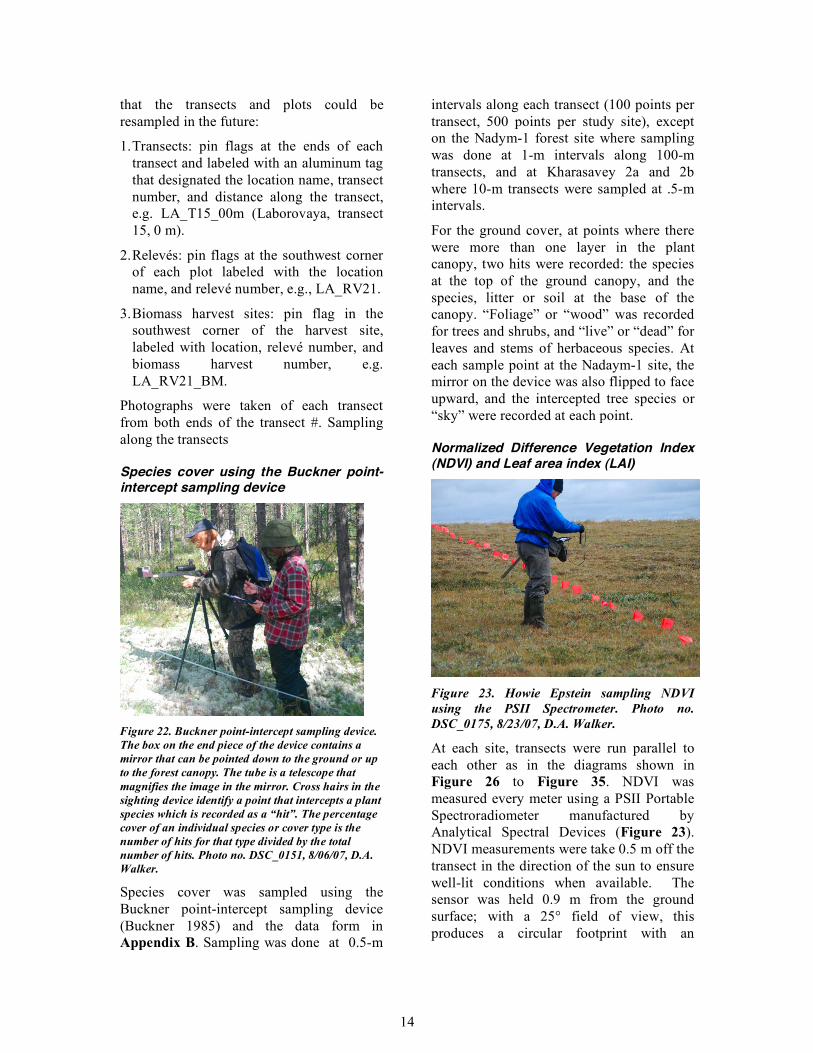
Figure 22. Buckner point-intercept sampling device. The box on the end piece of the device contains a mirror that can be pointed down to the ground or up to the forest canopy. The tube is a telescope that magnifies the image in the mirror. Cross hairs in the sighting device identify a point that intercepts a plant species which is recorded as a “hit”. The percentage cover of an individual species or cover type is the number of hits for that type divided by the total number of hits. Photo no. DSC_0151, 8/06/07, D.A. Walker.
Species cover was sampled using the Buckner point-intercept sampling device (Buckner 1985) and the data form in Appendix B. Sampling was done at 0.5-m
intervals along each transect (100 points per transect, 500 points per study site), except on the Nadym-1 forest site where sampling was done at 1-m intervals along 100-m transects, and at Kharasavey 2a and 2b where 10-m transects were sampled at .5-m intervals.
For the ground cover, at points where there were more than one layer in the plant canopy, two hits were recorded: the species at the top of the ground canopy, and the species, litter or soil at the base of the canopy. “Foliage” or “wood” was recorded for trees and shrubs, and “live” or “dead” for leaves and stems of herbaceous species. At each sample point at the Nadaym-1 site, the mirror on the device was also flipped to face upward, and the intercepted tree species or “sky” were recorded at each point.
Normalized Difference Vegetation Index (NDVI) and Leaf area index (LAI)
Figure 23. Howie Epstein sampling NDVI using the PSII Spectrometer. Photo no. DSC_0175, 8/23/07, D.A. Walker.
At each site, transects were run parallel to each other as in the diagrams shown in Figure 26 to Figure 35. NDVI was measured every meter using a PSII Portable Spectroradiometer manufactured by Analytical Spectral Devices (Figure 23). NDVI measurements were take 0.5 m off the transect in the direction of the sun to ensure well-lit conditions when available. The sensor was held 0.9 m from the ground surface; with a 25° field of view, this produces a circular footprint with an
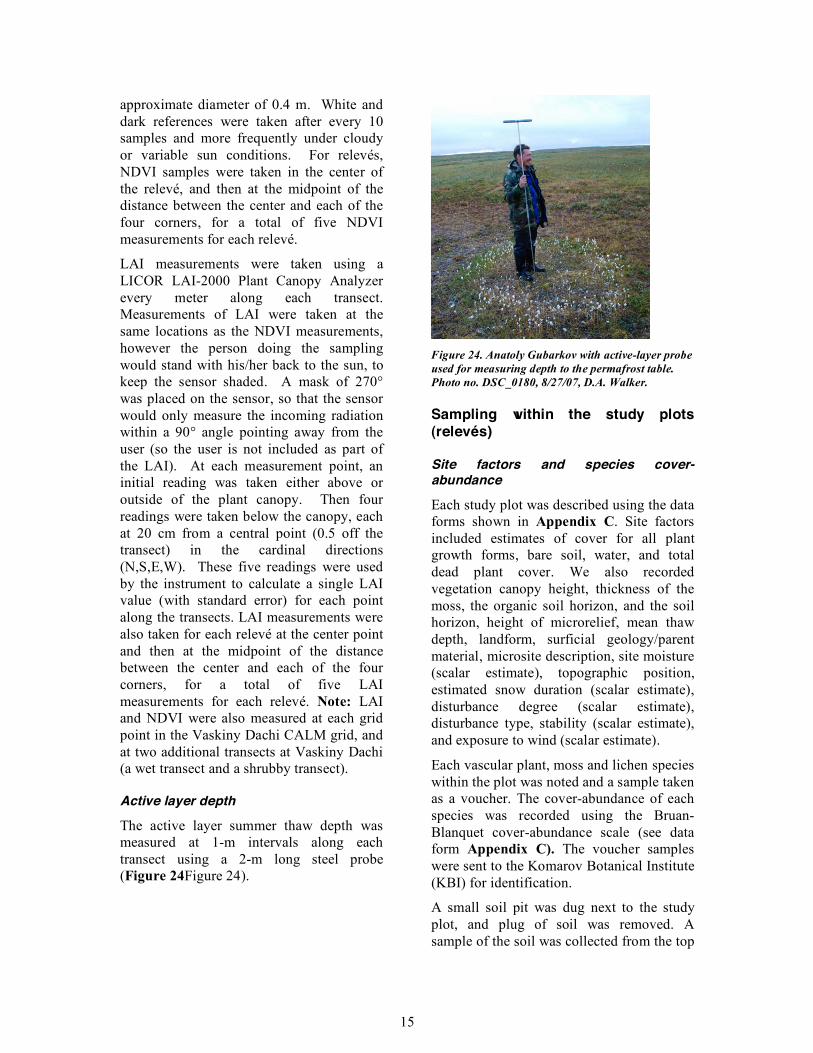
15
approximate diameter of 0.4 m. White and dark references were taken after every 10 samples and more frequently under cloudy or variable sun conditions. For relevés, NDVI samples were taken in the center of the relevé, and then at the midpoint of the distance between the center and each of the four corners, for a total of five NDVI measurements for each relevé.
LAI measurements were taken using a LICOR LAI-2000 Plant Canopy Analyzer every meter along each transect. Measurements of LAI were taken at the same locations as the NDVI measurements, however the person doing the sampling would stand with his/her back to the sun, to keep the sensor shaded. A mask of 270° was placed on the sensor, so that the sensor would only measure the incoming radiation within a 90° angle pointing away from the user (so the user is not included as part of the LAI). At each measurement point, an initial reading was taken either above or outside of the plant canopy. Then four readings were taken below the canopy, each at 20 cm from a central point (0.5 off the transect) in the cardinal directions (N,S,E,W). These five readings were used by the instrument to calculate a single LAI value (with standard error) for each point along the transects. LAI measurements were also taken for each relevé at the center point and then at the midpoint of the distance between the center and each of the four corners, for a total of five LAI measurements for each relevé. Note: LAI and NDVI were also measured at each grid point in the Vaskiny Dachi CALM grid, and at two additional transects at Vaskiny Dachi (a wet transect and a shrubby transect).
Active layer depth
The active layer summer thaw depth was measured at 1-m intervals along each transect using a 2-m long steel probe (Figure 24Figure 24).
Figure 24. Anatoly Gubarkov with active-layer probe used for measuring depth to the permafrost table. Photo no. DSC_0180, 8/27/07, D.A. Walker.
Sampling within the study plots (relevés)
Site factors and species cover-abundance
Each study plot was described using the data forms shown in Appendix C. Site factors included estimates of cover for all plant growth forms, bare soil, water, and total dead plant cover. We also recorded vegetation canopy height, thickness of the moss, the organic soil horizon, and the soil horizon, height of microrelief, mean thaw depth, landform, surficial geology/parent material, microsite description, site moisture (scalar estimate), topographic position, estimated snow duration (scalar estimate), disturbance degree (scalar estimate), disturbance type, stability (scalar estimate), and exposure to wind (scalar estimate).
Each vascular plant, moss and lichen species within the plot was noted and a sample taken as a voucher. The cover-abundance of each species was recorded using the Bruan-Blanquet cover-abundance scale (see data form Appendix C). The voucher samples were sent to the Komarov Botanical Institute (KBI) for identification.
A small soil pit was dug next to the study plot, and plug of soil was removed. A sample of the soil was collected from the top
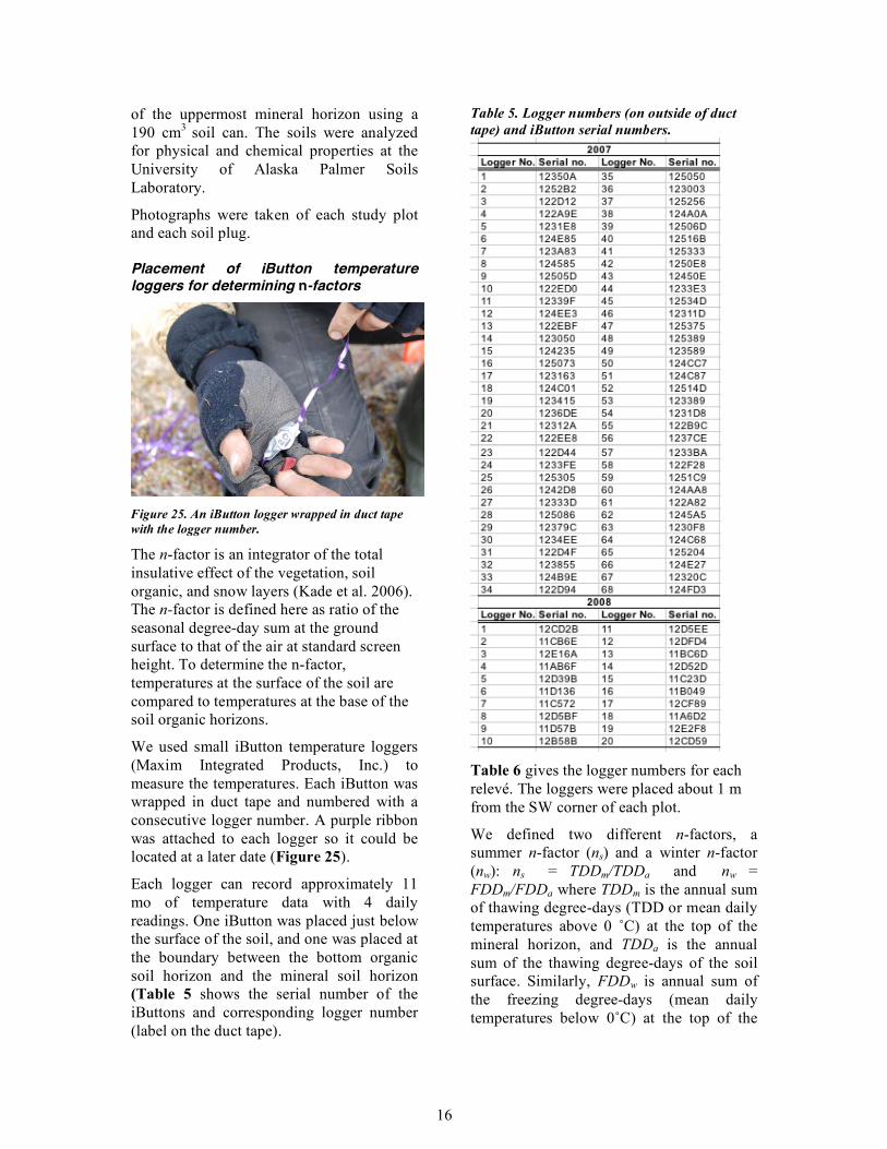
16
of the uppermost mineral horizon using a 190 cm3 soil can. The soils were analyzed for physical and chemical properties at the University of Alaska Palmer Soils Laboratory.
Photographs were taken of each study plot and each soil plug.
Placement of iButton temperature loggers for determining n-factors
Figure 25. An iButton logger wrapped in duct tape with the logger number.
The n-factor is an integrator of the total insulative effect of the vegetation, soil organic, and snow layers (Kade et al. 2006). The n-factor is defined here as ratio of the seasonal degree-day sum at the ground surface to that of the air at standard screen height. To determine the n-factor, temperatures at the surface of the soil are compared to temperatures at the base of the soil organic horizons.
We used small iButton temperature loggers (Maxim Integrated Products, Inc.) to measure the temperatures. Each iButton was wrapped in duct tape and numbered with a consecutive logger number. A purple ribbon was attached to each logger so it could be located at a later date (Figure 25).
Each logger can record approximately 11 mo of temperature data with 4 daily readings. One iButton was placed just below the surface of the soil, and one was placed at the boundary between the bottom organic soil horizon and the mineral soil horizon (Table 5 shows the serial number of the iButtons and corresponding logger number (label on the duct tape).
Table 5. Logger numbers (on outside of duct tape) and iButton serial numbers.
Table 6 gives the logger numbers for each relevé. The loggers were placed about 1 m from the SW corner of each plot.
We defined two different n-factors, a summer n-factor (ns) and a winter n-factor (nw): ns = TDDm/TDDa and nw = FDDm/FDDa where TDDm is the annual sum of thawing degree-days (TDD or mean daily temperatures above 0 ˚C) at the top of the mineral horizon, and TDDa is the annual sum of the thawing degree-days of the soil surface. Similarly, FDDw is annual sum of the freezing degree-days (mean daily temperatures below 0˚C) at the top of the
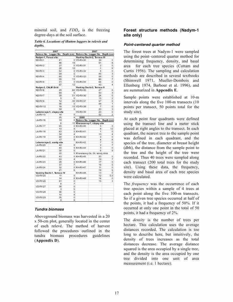
17
mineral soil, and FDDa is the freezing degree-days at the soil surface. Table 6. Locations of iButton loggers in relevés and depths.
Tundra biomass
Aboveground biomass was harvested in a 20 x 50-cm plot, generally located in the center of each relevé. The method of harvest followed the procedures outlined in the tundra biomass procedures guidelines (Appendix D).
Forest structure methods (Nadym-1 site only)
Point-centered quarter method The forest trees at Nadym-1 were sampled using the point–centered quarter method for determining frequency, density, and basal area for each tree species (Cottam and Curtis 1956). The sampling and calculation methods are described in several textbooks (Shimwell 1971, Mueller-Dombois and Ellenberg 1974, Barbour et al. 1996), and are summarized in Appendix E. Sample points were established at 10-m intervals along the five 100-m transects (10 points per transect, 50 points total for the study site).
At each point four quadrants were defined using the transect line and a meter stick placed at right angles to the transect. In each quadrant, the nearest tree to the sample point was defined in each quadrant, and the species of the tree, diameter at breast height (dbh), the distance from the sample point to the tree and the height of the tree were recorded. Thus 40 trees were sampled along each transect (200 total trees for the study site). Using these data, the frequency, density and basal area of each tree species were calculated.
The frequency was the occurrence of each tree species within a sample of 4 trees at each point along the five 100-m transects. So if a given tree species occurred at half of the points, it had a frequency of 50%. If it occurred at only one point in the total of 50 points, it had a frequency of 2%.
The density is the number of trees per hectare. This calculation uses the average distances recorded. The calculation is too long to describe here, but intuitively, the density of trees increases as the total distances decrease. The average distance squared is the area occupied by a single tree, and the density is the area occupied by one tree divided into one unit of area measurement (i.e. 1 hectare).

18
The basal area is the area of the tree stems at breast height per hectare. This calculation uses the density of each tree species and areas of the measured stems.
Plot-count method: In each 10 x 10-m plot, the location of each tree was recorded using coordinates in meters. The position of each tree was estimated to nearest 0.25 m by running a 10-m tape along each border of the plot, using the SW corner of the plot as the origin. For each tree the species, diameter at breast height and the height of the tree were recorded. The number of samplings (dbh < 5 cm) and number of seedlings of each species were also recorded.
Using these data the density and basal area of each tree species within each plot were determined.
Tree biomass Tree biomass was determined for the forest using both the data from the point-centered quarter method and the plot-count method. Aboveground tree biomasses were calculated using following equations (Zianis et al. 2005):
Betula pubescens (equation no. 40, Zianis et al. 2005):
Biomass [kg] = a * Db , where a = 0.00029, b = 2.50038, D = diameter at breast height [mm]
Pinus sylvestris (equation no. 388, Zianis et al. 2005):
Biomass [kg] = a + b*D + c*D2 , where
a = 18,779; b = (-4,328); c = 0.506; D = diameter at breast height [cm]
Larix sibirica (equation no. 136, Zianis et al. 2005):
Biomass [kg] = a * Db * Hc, where
a = 0.1081; b = 1.53; c = 0.9482; D = diameter at breast height [cm]; H = height [m].
Pinus sibirica (equation no. 733. Muukkonen et al. 2006):
Biomass [kg] = a + b*D2 *H + c*D2, where
a = (-3.4268); b = 0.010356; c = 0.14144; D = diameter at breast height [cm]; H = height [m].
Biomass for both Pinus sylvestris and P. sibirica saplings (dbh < 5 cm) (equation no. 327 (Zianis et al. 2005). Note: Because there are few equations available for estimating biomass of young trees, the following equation was used.
Biomass [kg] = a * exp(D*b), where
a = 0.2304; b = 0.6536; D = diameter at breast height [cm].
Tree cover, density, and basal area using the plot-count method (Nadym-1 forest site only) For each of the five 10 x 10 m relevés at the forest site at Nadym, each individual tree was mapped and the diameter at breast height measured and height visually estimated. In addition the number of seedlings for each species was counted for each relevé.
Soils Two types of soils data were collected: (1) Relevé soil samples: A sample of soil was collected from each of the 39 study plots (relevés) at the top of the top mineral horizon using a 190 cm3 soil can. These soil samples are being analyzed at the University of Alaska for physical and chemical properties. (2) Soil pit: One or two soil pits were dug at each site, in a representative site, usually near the southwest corner of the site. These pits were described by Dr. Georgy Matyshak according the Russian approach and translated into descriptions corresponding to the US Soil Taxonomy approach of soil description (see Soil Descriptions of Study Sites: G. Matyshak).
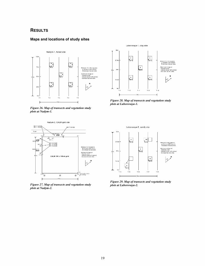
19
RESULTS
Maps and locations of study sites
Figure 26. Map of transects and vegetation study plots at Nadym-1.
Figure 27. Map of transects and vegetation study plots at Nadym-2.
Figure 28. Map of transects and vegetation study plots at Laborovaya-1.
Figure 29. Map of transects and vegetation study plots at Laborovaya-2.
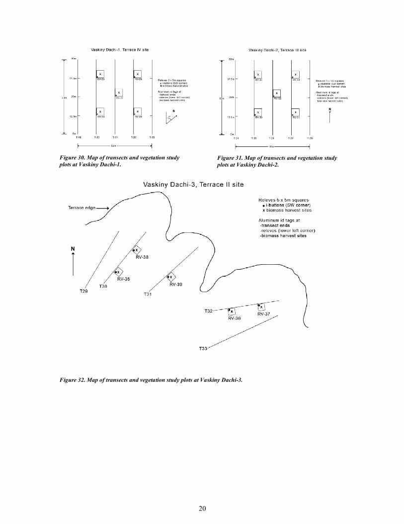
20
Figure 30. Map of transects and vegetation study plots at Vaskiny Dachi-1.
Figure 31. Map of transects and vegetation study plots at Vaskiny Dachi-2.
Figure 32. Map of transects and vegetation study plots at Vaskiny Dachi-3.
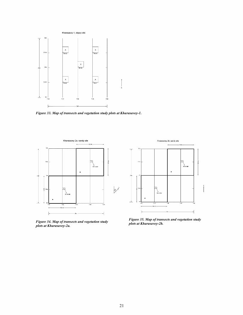
21
Figure 33. Map of transects and vegetation study plots at Kharasavey-1.
Figure 34. Map of transects and vegetation study plots at Kharasavey-2a.
Figure 35. Map of transects and vegetation study plots at Kharasavey-2b.
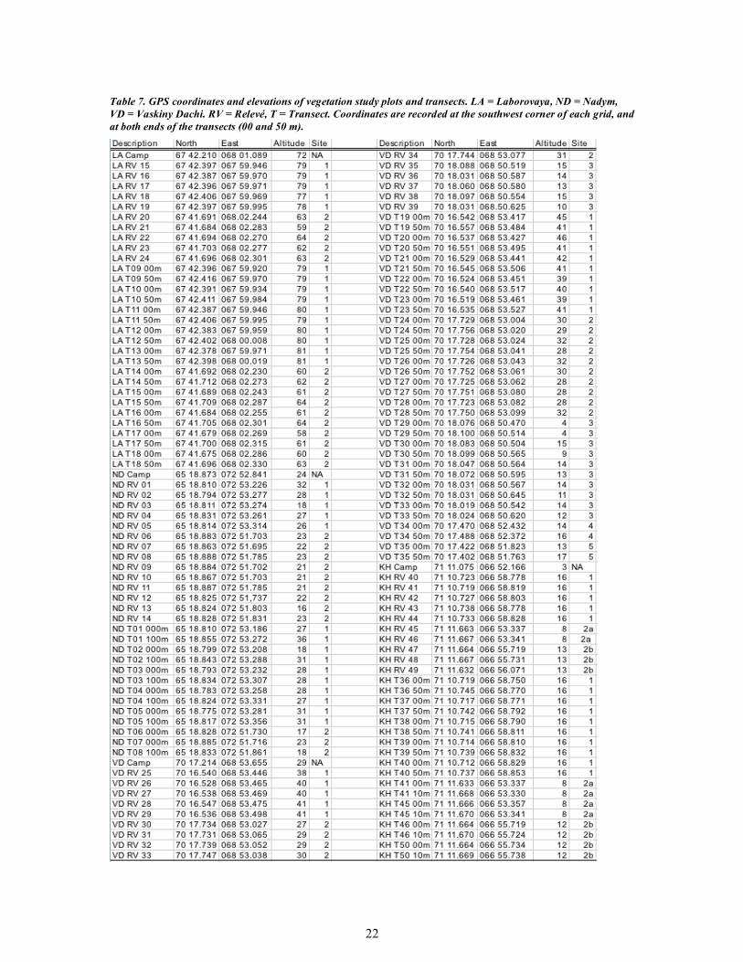
22
Table 7. GPS coordinates and elevations of vegetation study plots and transects. LA = Laborovaya, ND = Nadym, VD = Vaskiny Dachi. RV = Relevé, T = Transect. Coordinates are recorded at the southwest corner of each grid, and at both ends of the transects (00 and 50 m).
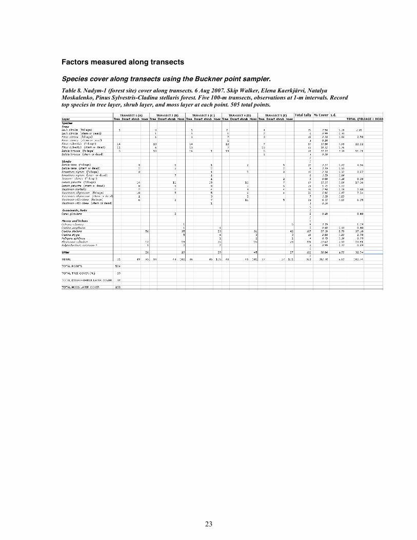
23
Factors measured along transects
Species cover along transects using the Buckner point sampler. Table 8. Nadym-1 (forest site) cover along transects. 6 Aug 2007. Skip Walker, Elena Kaerkjärvi, Natalya Moskalenko, Pinus Sylvestris-Cladina stellaris forest. Five 100-m transects, observations at 1-m intervals. Record top species in tree layer, shrub layer, and moss layer at each point. 505 total points.

24
Table 9. Nadym-2 (CALM-grid site) cover along transect. “Overstory” species are those recorded at the top of the plant canopy at each point; “understory” species are those recorded at the base of the plant canopy; (l) - live green plant part, (d) – dead or senescent plant part. Species use six letter abbreviations. Only two transects were sampled at Nadym-2 because of the limited area available for sampling. Sample points were identified as one of three microsites: hummocks, inter-hummocks, and wet inter-hummocks.
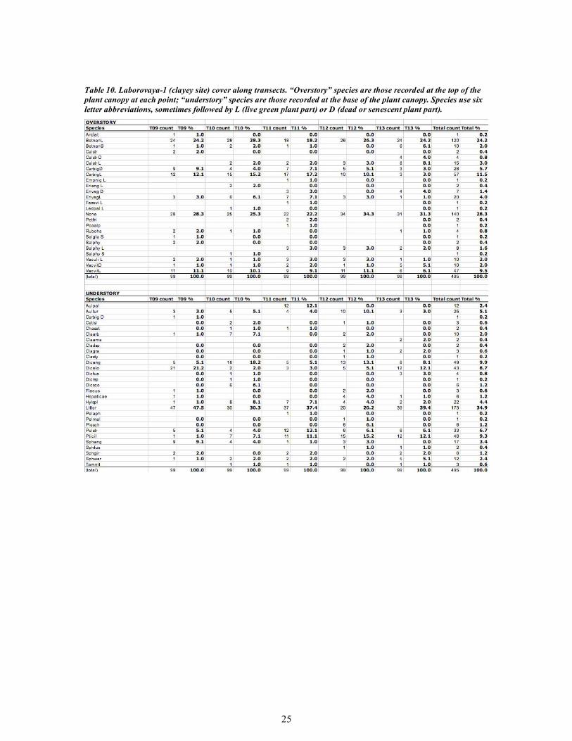
25
Table 10. Laborovaya-1 (clayey site) cover along transects. “Overstory” species are those recorded at the top of the plant canopy at each point; “understory” species are those recorded at the base of the plant canopy. Species use six letter abbreviations, sometimes followed by L (live green plant part) or D (dead or senescent plant part).
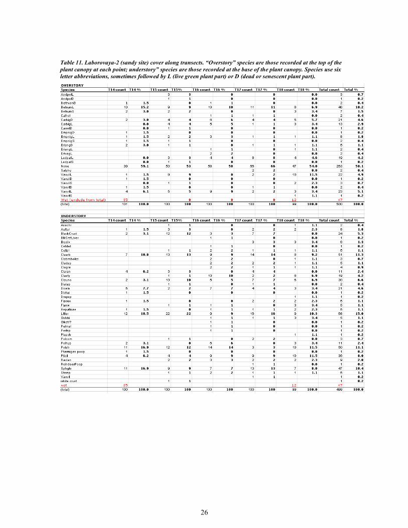
26
Table 11. Laborovaya-2 (sandy site) cover along transects. “Overstory” species are those recorded at the top of the plant canopy at each point; understory” species are those recorded at the base of the plant canopy. Species use six letter abbreviations, sometimes followed by L (live green plant part) or D (dead or senescent plant part).
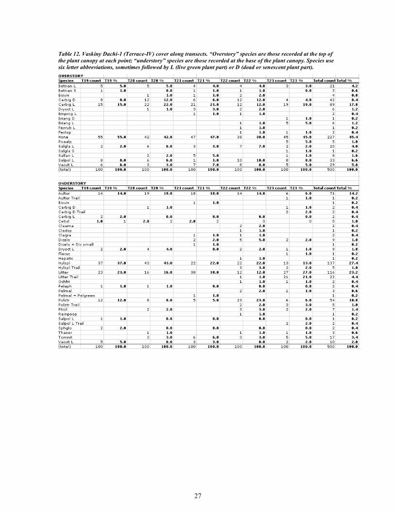
27
Table 12. Vaskiny Dachi-1 (Terrace-IV) cover along transects. “Overstory” species are those recorded at the top of the plant canopy at each point; “understory” species are those recorded at the base of the plant canopy. Species use six letter abbreviations, sometimes followed by L (live green plant part) or D (dead or senescent plant part).
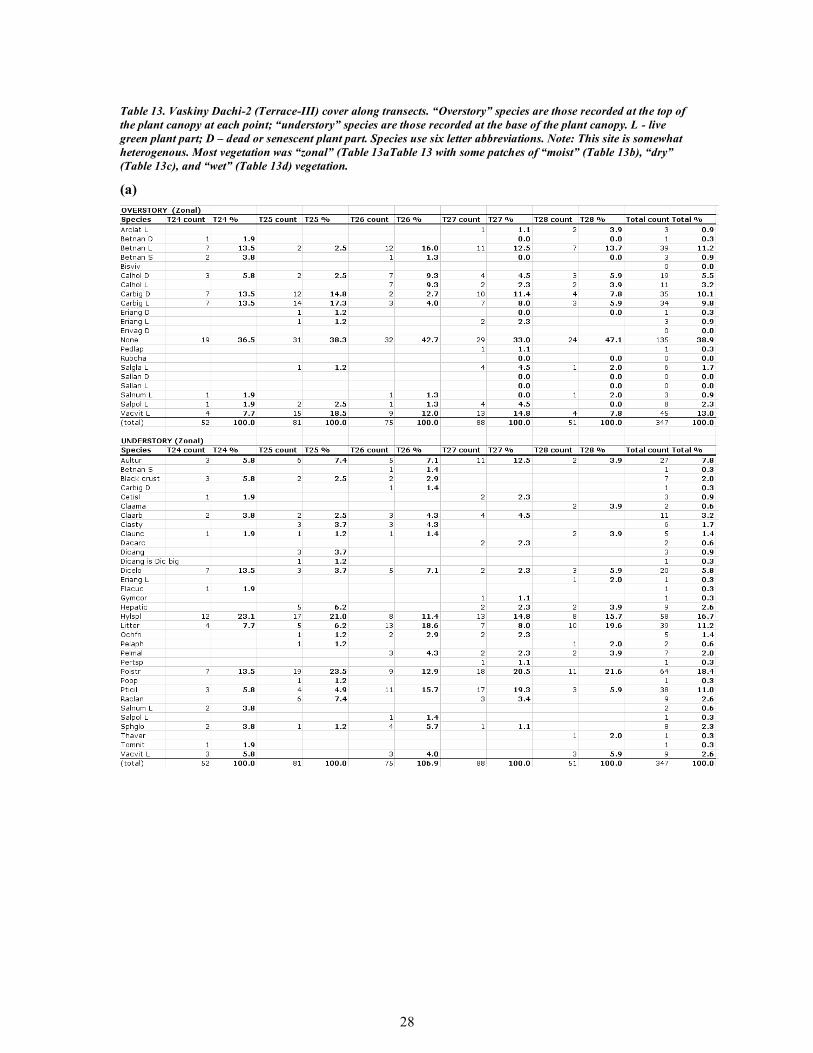
28
Table 13. Vaskiny Dachi-2 (Terrace-III) cover along transects. “Overstory” species are those recorded at the top of the plant canopy at each point; “understory” species are those recorded at the base of the plant canopy. L - live green plant part; D – dead or senescent plant part. Species use six letter abbreviations. Note: This site is somewhat heterogenous. Most vegetation was “zonal” (Table 13aTable 13 with some patches of “moist” (Table 13b), “dry” (Table 13c), and “wet” (Table 13d) vegetation.
(a)
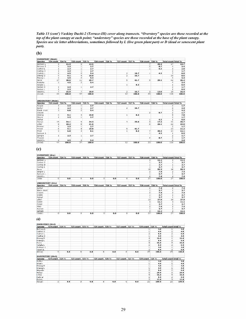
29
Table 13 (cont’) Vaskiny Dachi-2 (Terrace-III) cover along transects. “Overstory” species are those recorded at the top of the plant canopy at each point; “understory” species are those recorded at the base of the plant canopy. Species use six letter abbreviations, sometimes followed by L (live green plant part) or D (dead or senescent plant part).
(b)
(c)
(d)
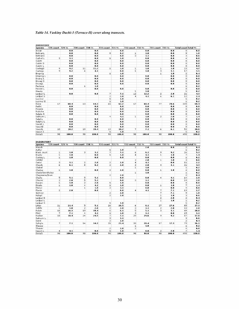
30
Table 14. Vaskiny Dachi-3 (Terrace-II) cover along transects.
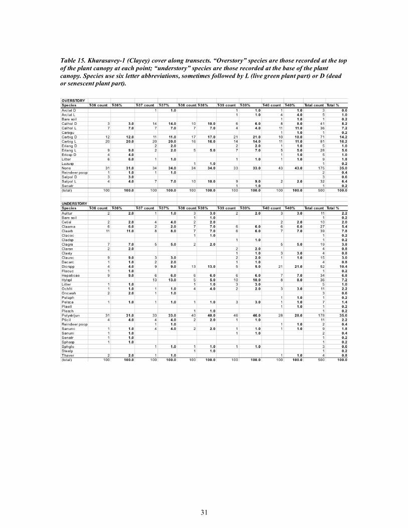
31
Table 15. Kharasavey-1 (Clayey) cover along transects. “Overstory” species are those recorded at the top of the plant canopy at each point; “understory” species are those recorded at the base of the plant canopy. Species use six letter abbreviations, sometimes followed by L (live green plant part) or D (dead or senescent plant part).
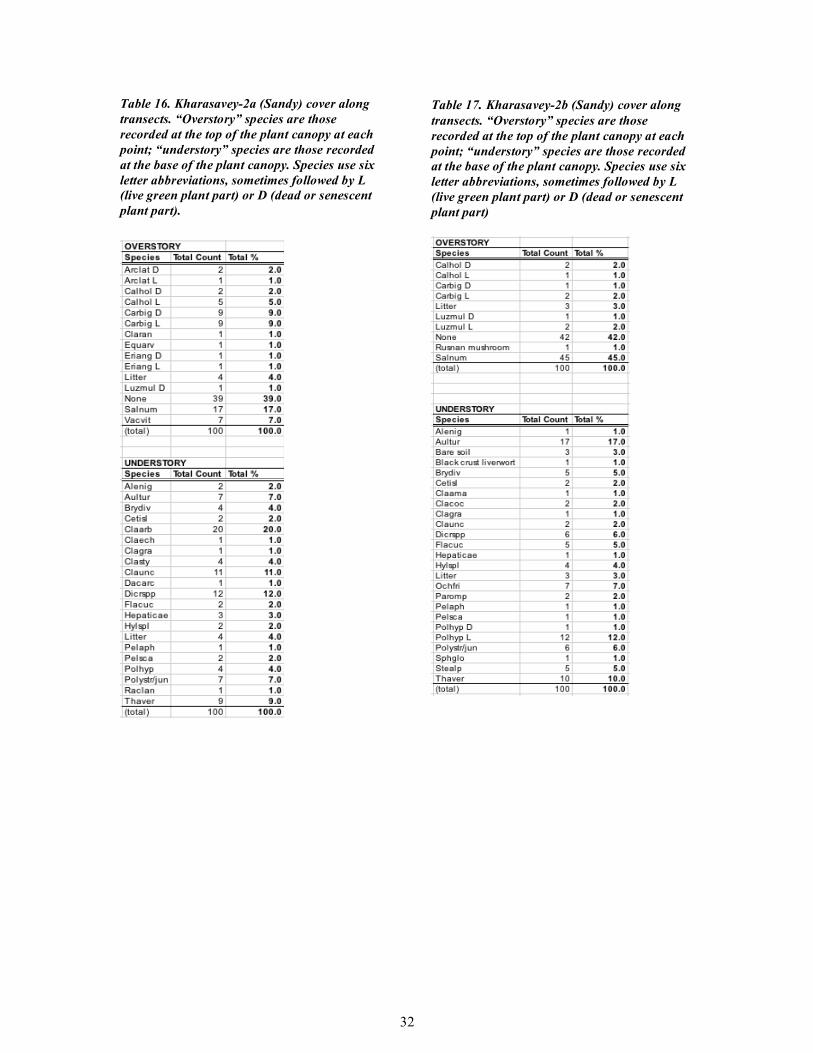
32
Table 16. Kharasavey-2a (Sandy) cover along transects. “Overstory” species are those recorded at the top of the plant canopy at each point; “understory” species are those recorded at the base of the plant canopy. Species use six letter abbreviations, sometimes followed by L (live green plant part) or D (dead or senescent plant part).
Table 17. Kharasavey-2b (Sandy) cover along transects. “Overstory” species are those recorded at the top of the plant canopy at each point; “understory” species are those recorded at the base of the plant canopy. Species use six letter abbreviations, sometimes followed by L (live green plant part) or D (dead or senescent plant part)
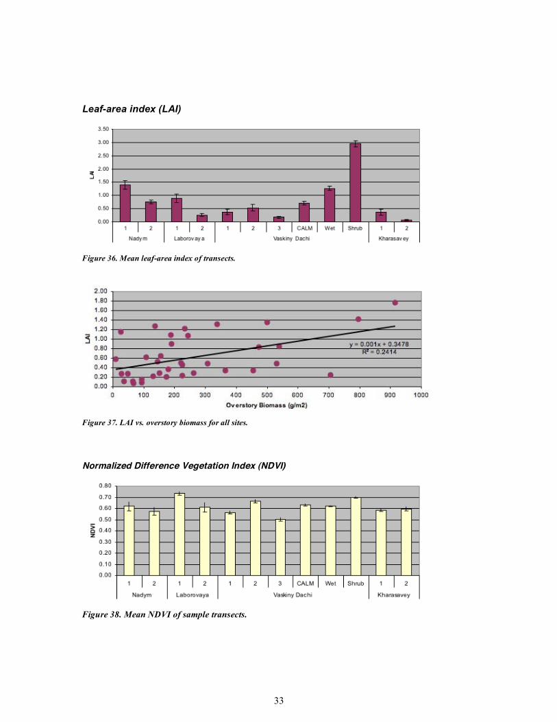
33
Leaf-area index (LAI)
Figure 36. Mean leaf-area index of transects.
Figure 37. LAI vs. overstory biomass for all sites.
Normalized Difference Vegetation Index (NDVI)
Figure 38. Mean NDVI of sample transects.

34
Figure 39. NDVI vs. LAI for all transects.
Figure 40. NDVI vs biomass for all sites.
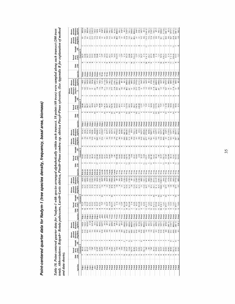
35
Poin
t-cen
tere
d qu
arte
r dat
a fo
r Nad
ym-1
(tre
e sp
ecie
s de
nsity
, fre
quen
cy, b
asal
are
a, b
iom
ass)
Tabl
e 18
. Poi
nt-c
ente
red
quar
ter d
ata
for N
adym
-1 w
ith sp
ecie
s arr
ange
d al
phab
etic
ally
with
in e
ach
trans
ect.
10 p
oint
s (40
tree
s) w
ere
sam
pled
alo
ng e
ach
trans
ect (
200
tree
s to
tal).
Abb
revi
atio
ns: B
etpu
b= B
etul
a pu
besc
ens,
Lars
ib=L
arix
sibi
rica
, Pin
sib=P
inus
cem
bra
ssp.
sibi
rica
Pin
syl=
Pinu
s syl
vest
ris.
(See
App
endi
x B
for e
xpla
natio
n of
met
hod
and
data
shee
ts).
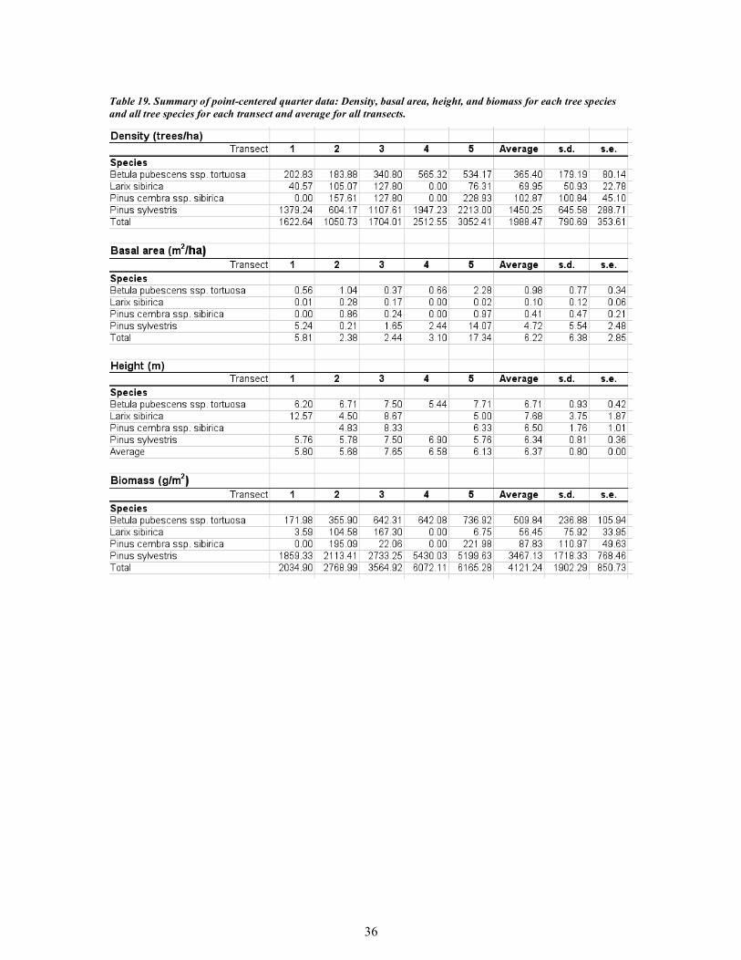
36
Table 19. Summary of point-centered quarter data: Density, basal area, height, and biomass for each tree species and all tree species for each transect and average for all transects.
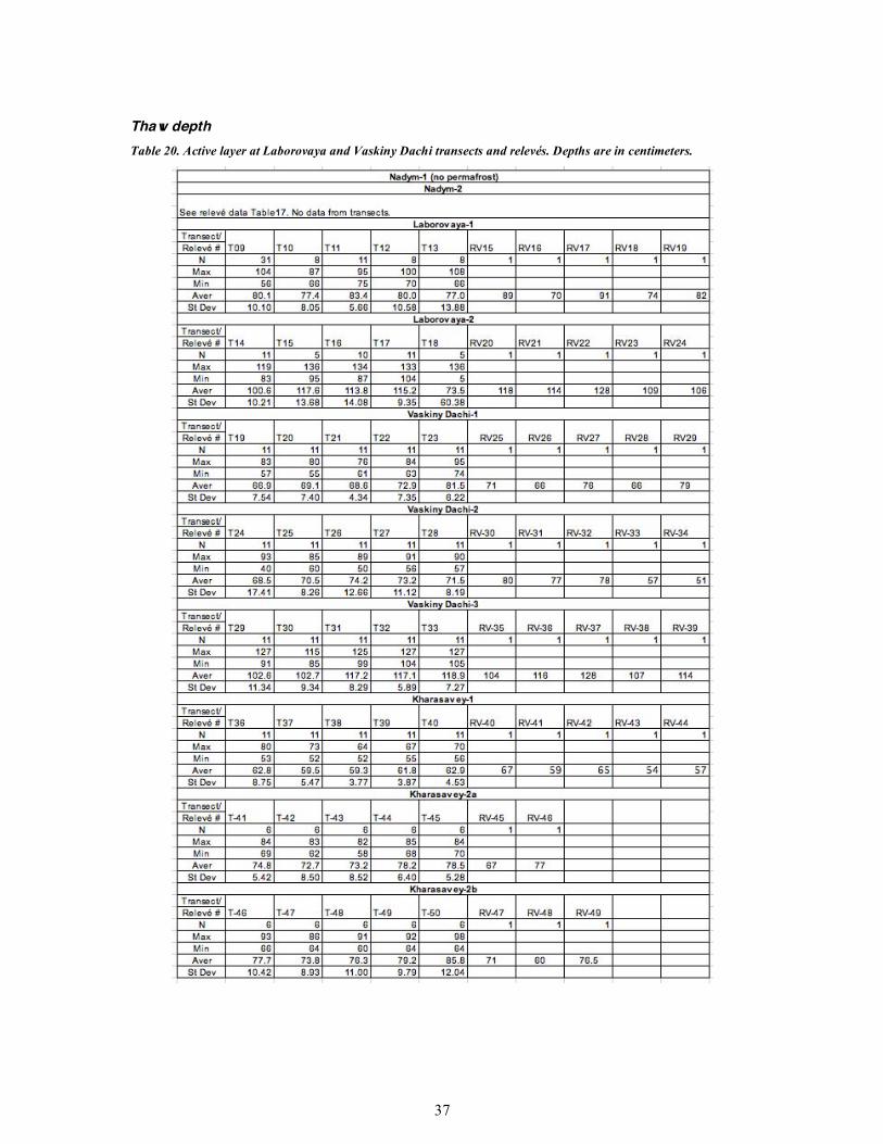
37
Thaw depth Table 20. Active layer at Laborovaya and Vaskiny Dachi transects and relevés. Depths are in centimeters.
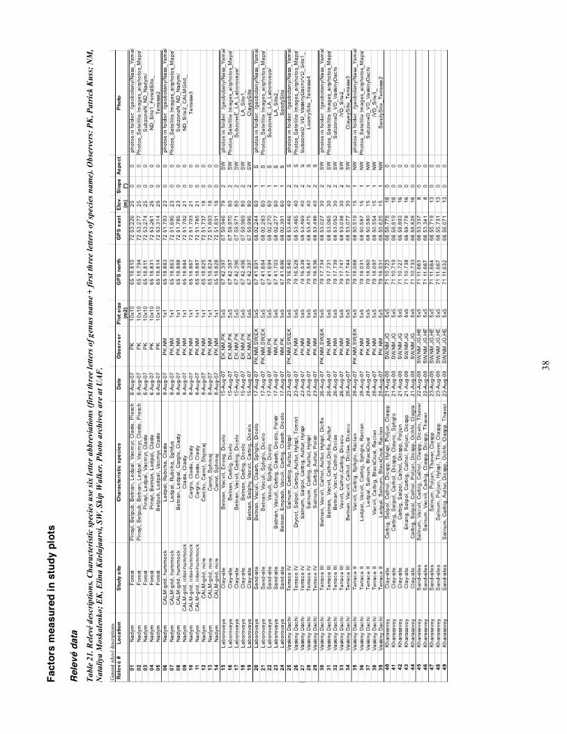
38
Fact
ors
mea
sure
d in
stu
dy p
lots
Rele
vé d
ata
Tabl
e 21
. Rel
evé
desc
riptio
ns. C
hara
cter
istic
spec
ies u
se si
x le
tter a
bbre
viat
ions
(fir
st th
ree
lette
rs o
f gen
us n
ame
+ fir
st th
ree
lette
rs o
f spe
cies
nam
e). O
bser
vers
: PK
, Pat
rick
Kus
s; N
M,
Nat
aliy
a M
oska
lenk
o; E
K, E
lina
Kär
laja
arvi
, SW
, Ski
p W
alke
r. Ph
oto
arch
ives
are
at U
AF
.
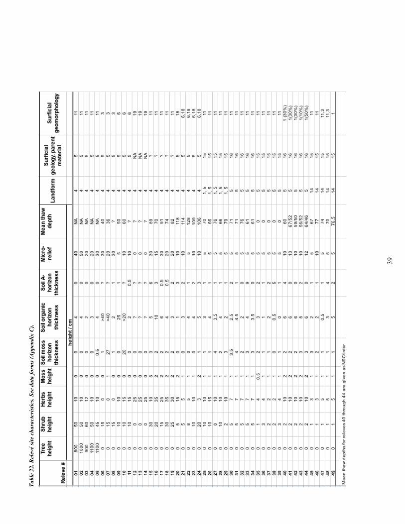
39
Tabl
e 22
. Rel
evé
site
cha
ract
eris
tics.
See
data
form
s (A
ppen
dix
C).
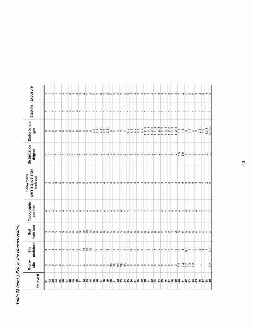
40
Tabl
e 22
(con
t’) R
elev
é si
te c
hara
cter
istic
s.
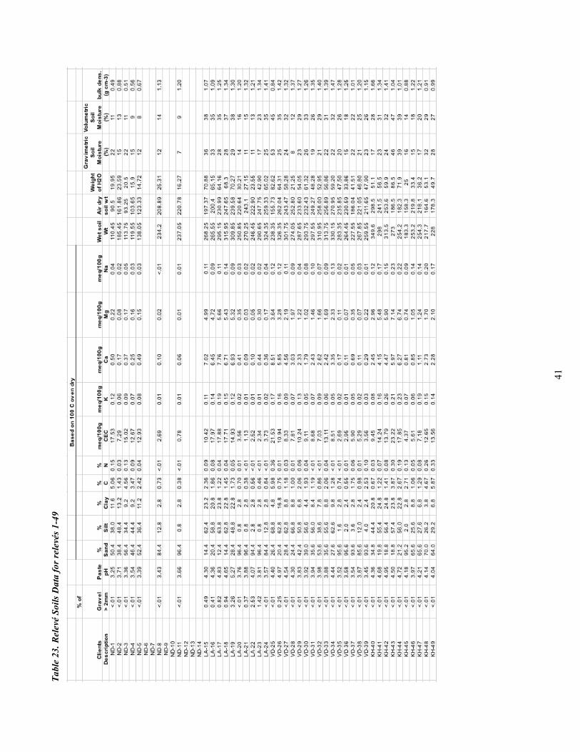
41
Tabl
e 23
. Rel
evé
Soils
Dat
a fo
r rel
evés
1-4
9
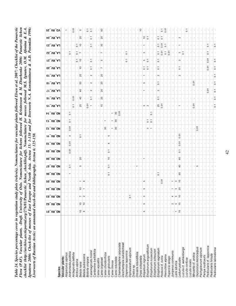
42
Tabl
e 24
. Spe
cies
per
cent
age
cove
r in
vege
tatio
n st
udy
plot
s (re
levé
s). N
omen
clat
ure
for v
ascu
lar p
lant
s fol
low
ed E
lven
et a
l. 20
07: C
heck
list o
f the
Pan
arct
ic
Flor
a (P
AF)
. Va
scul
ar p
lant
s. -D
raft.
Uni
vers
ity o
f O
slo.
Nom
encl
atur
e fo
r lic
hens
fol
low
ed H
. Kr
istin
sson
& M
. Zh
urbe
nko
2006
: Pa
narc
tic l
iche
n ch
eckl
ist (
http
://ar
chiv
e.ar
ctic
port
al.o
rg/2
76/0
1/Pa
narc
tic_l
iche
n_ch
eckl
ist.p
df).
Nom
encl
atur
e fo
r m
osse
s fo
llowe
d M
.S.
Igna
tov,
O.M
. Af
onin
a &
E.A
. Ig
nato
va 2
006:
Che
ck-li
st o
f m
osse
s of
Eas
t Eu
rope
and
Nor
th A
sia.
Arct
oa 1
5: 1
-130
and
for
liv
erwo
rts
N.A
. K
onsta
ntin
ova
& A
.D.
Pote
mki
n 19
96:
Live
rwor
ts of
Rus
sian
Arct
ic: a
n an
nota
ted
chec
k-lis
t and
bib
liogr
aphy
. Arc
toa
6: 1
25-1
50.
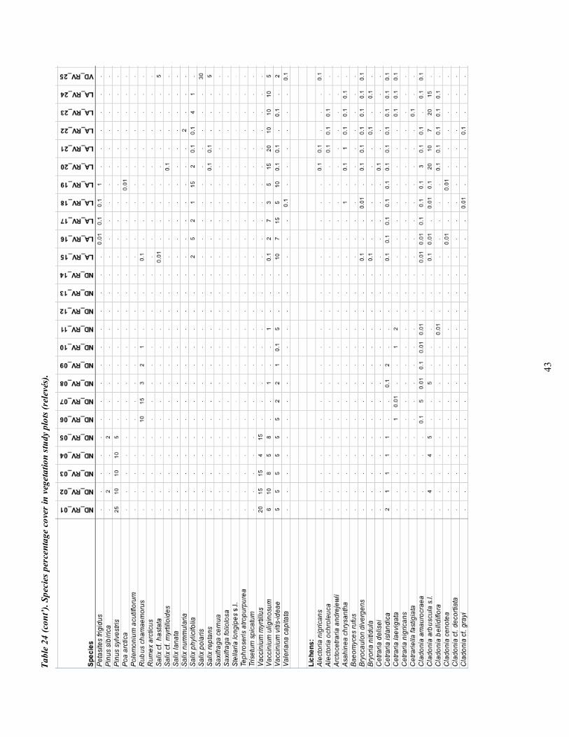
43
Tabl
e 24
(con
t’). S
peci
es p
erce
ntag
e co
ver i
n ve
geta
tion
stud
y pl
ots (
rele
vés)
.
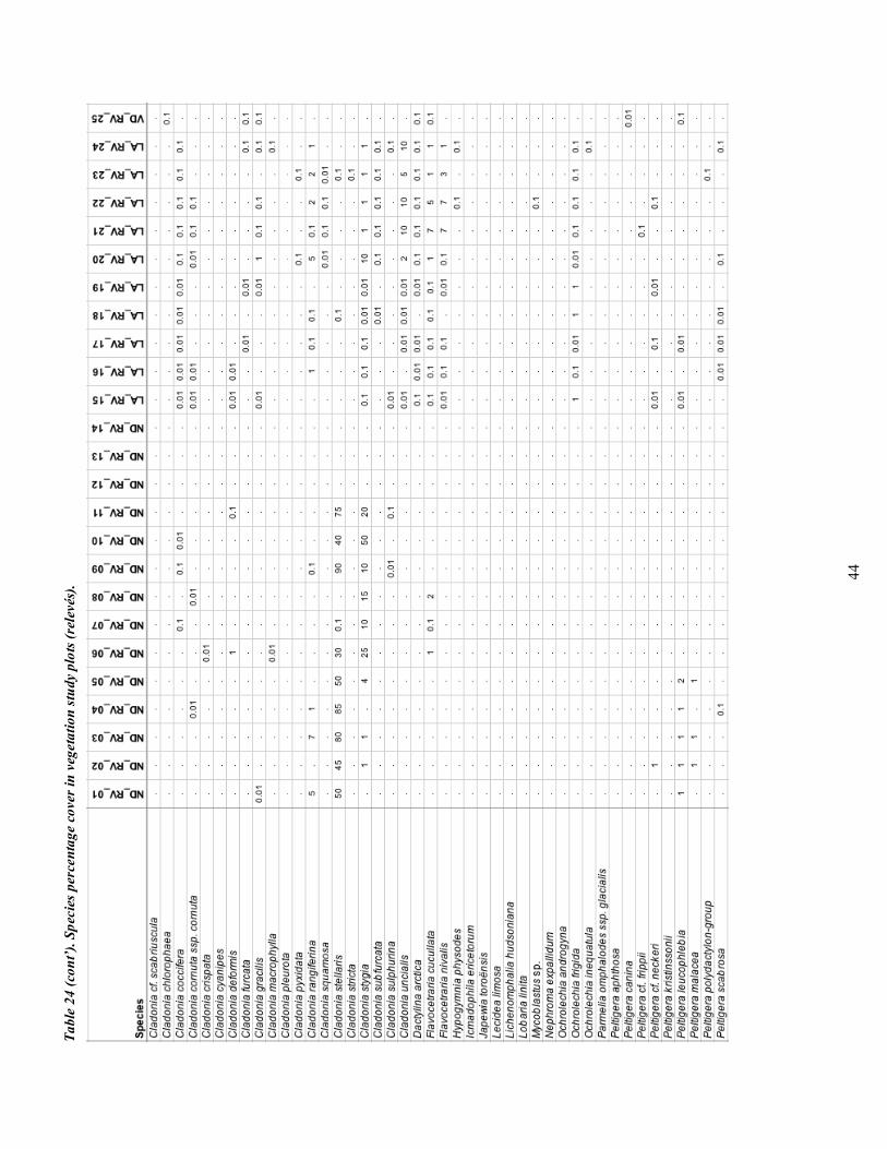
44
Tabl
e 24
(con
t’). S
peci
es p
erce
ntag
e co
ver i
n ve
geta
tion
stud
y pl
ots (
rele
vés)
.
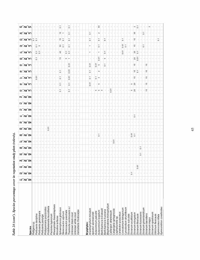
45
Tabl
e 24
(con
t’). S
peci
es p
erce
ntag
e co
ver i
n ve
geta
tion
stud
y pl
ots (
rele
vés)
.
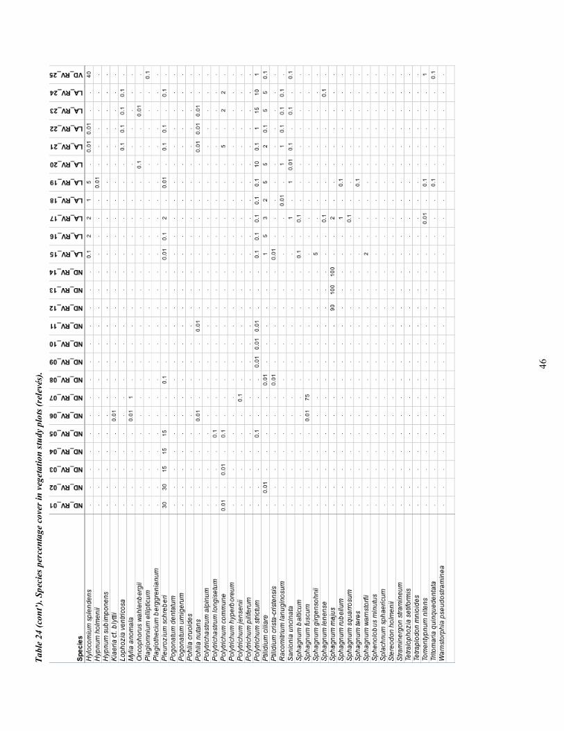
46
Tabl
e 24
(con
t’). S
peci
es p
erce
ntag
e co
ver i
n ve
geta
tion
stud
y pl
ots (
rele
vés)
.
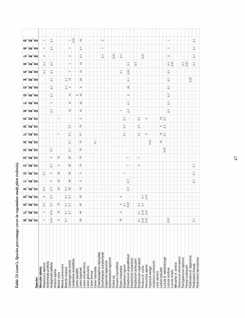
47
Tabl
e 24
(con
t’). S
peci
es p
erce
ntag
e co
ver i
n ve
geta
tion
stud
y pl
ots (
rele
vés)
.
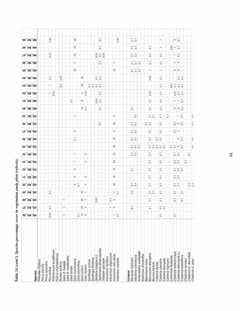
48
Tabl
e 24
(con
t’). S
peci
es p
erce
ntag
e co
ver i
n ve
geta
tion
stud
y pl
ots (
rele
vés)
.
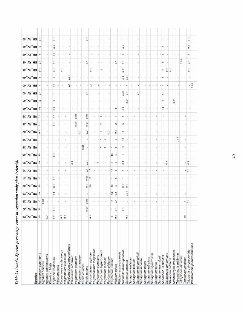
49
Tabl
e 24
(con
t’). S
peci
es p
erce
ntag
e co
ver i
n ve
geta
tion
stud
y pl
ots (
rele
vés)
.
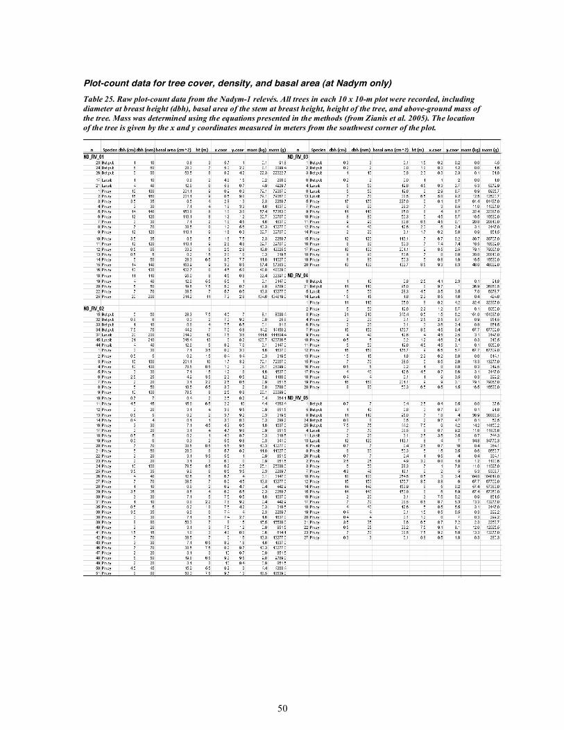
50
Plot-count data for tree cover, density, and basal area (at Nadym only) Table 25. Raw plot-count data from the Nadym-1 relevés. All trees in each 10 x 10-m plot were recorded, including diameter at breast height (dbh), basal area of the stem at breast height, height of the tree, and above-ground mass of the tree. Mass was determined using the equations presented in the methods (from Zianis et al. 2005). The location of the tree is given by the x and y coordinates measured in meters from the southwest corner of the plot.
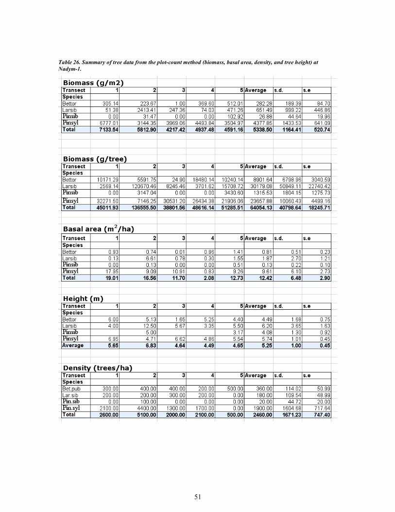
51
Table 26. Summary of tree data from the plot-count method (biomass, basal area, density, and tree height) at Nadym-1.
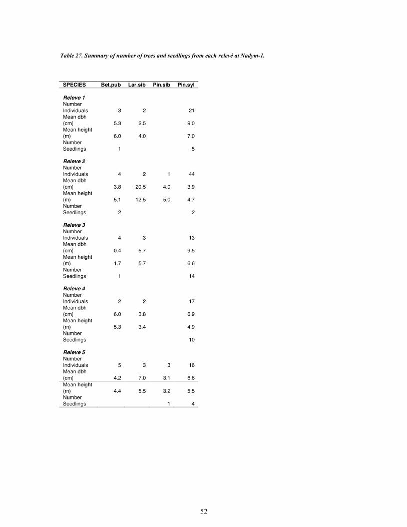
52
Table 27. Summary of number of trees and seedlings from each relevé at Nadym-1.
SPECIES Bet.pub Lar.sib Pin.sib Pin.syl Releve 1 Number Individuals 3 2 21 Mean dbh (cm) 5.3 2.5 9.0 Mean height (m) 6.0 4.0 7.0 Number Seedlings 1 5 Releve 2 Number Individuals 4 2 1 44 Mean dbh (cm) 3.8 20.5 4.0 3.9 Mean height (m) 5.1 12.5 5.0 4.7 Number Seedlings 2 2 Releve 3 Number Individuals 4 3 13 Mean dbh (cm) 0.4 5.7 9.5 Mean height (m) 1.7 5.7 6.6 Number Seedlings 1 14 Releve 4 Number Individuals 2 2 17 Mean dbh (cm) 6.0 3.8 6.9 Mean height (m) 5.3 3.4 4.9 Number Seedlings 10 Releve 5 Number Individuals 5 3 3 16 Mean dbh (cm) 4.2 7.0 3.1 6.6 Mean height (m) 4.4 5.5 3.2 5.5 Number Seedlings 1 4
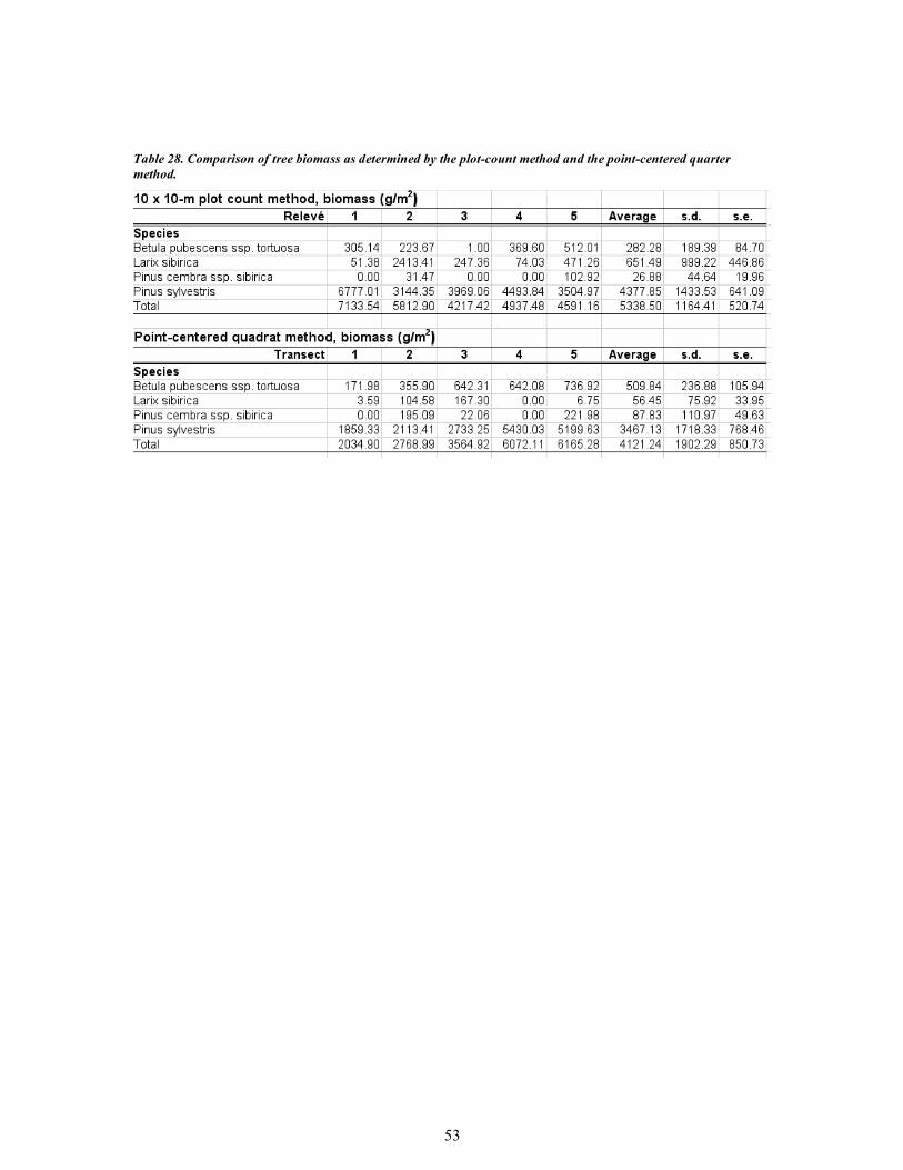
53
Table 28. Comparison of tree biomass as determined by the plot-count method and the point-centered quarter method.
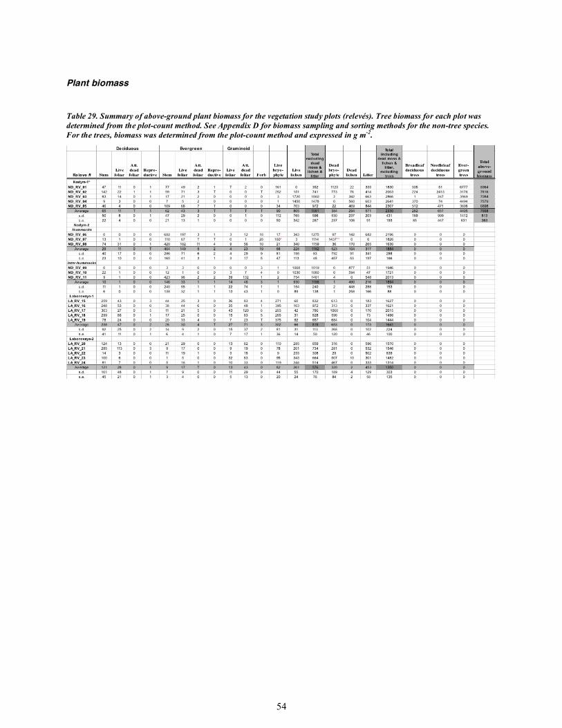
54
Plant biomass
Table 29. Summary of above-ground plant biomass for the vegetation study plots (relevés). Tree biomass for each plot was determined from the plot-count method. See Appendix D for biomass sampling and sorting methods for the non-tree species. For the trees, biomass was determined from the plot-count method and expressed in g m-2.
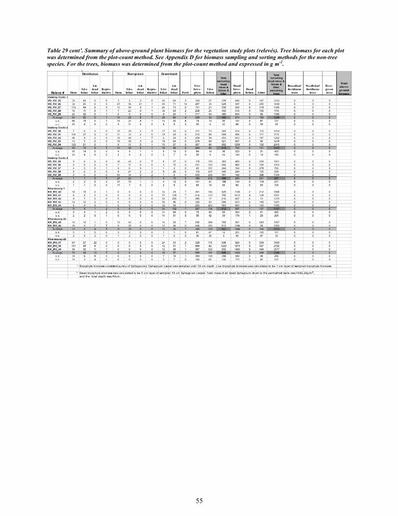
55
Table 29 cont’. Summary of above-ground plant biomass for the vegetation study plots (relevés). Tree biomass for each plot was determined from the plot-count method. See Appendix D for biomass sampling and sorting methods for the non-tree species. For the trees, biomass was determined from the plot-count method and expressed in g m-2.
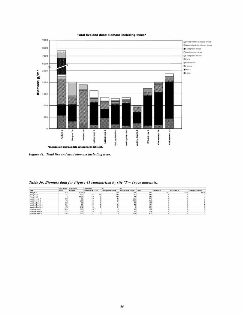
56
Figure 41. Total live and dead biomass including trees.
Table 30. Biomass data for Figure 41 summarized by site (T = Trace amounts).
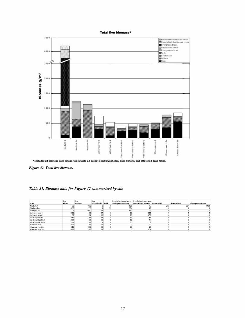
57
Figure 42. Total live biomass.
Table 31. Biomass data for Figure 42 summarized by site
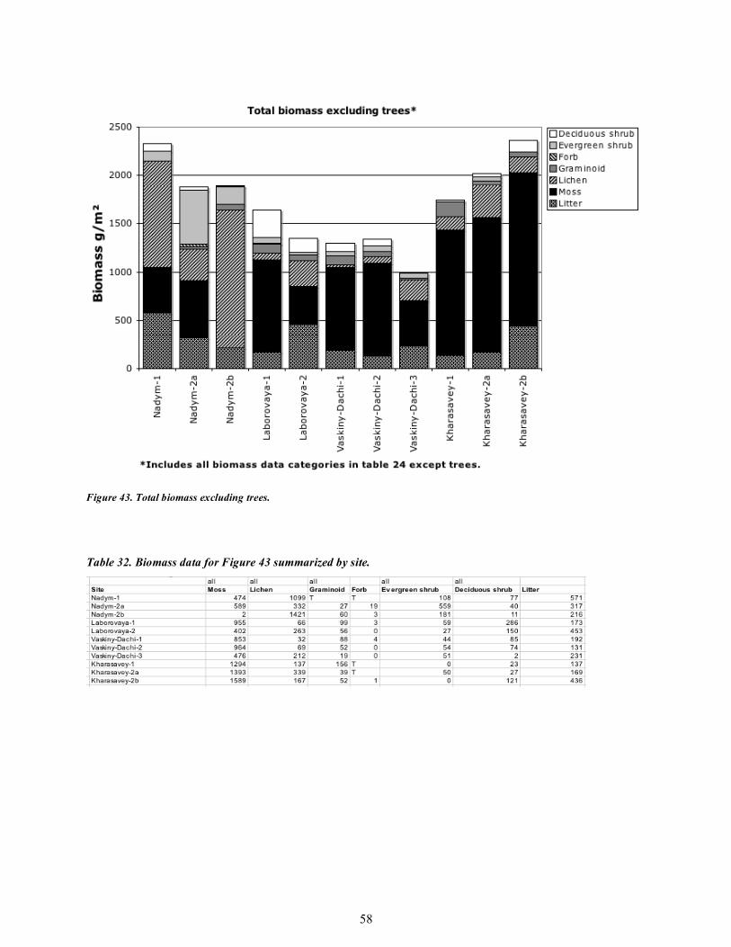
58
Figure 43. Total biomass excluding trees.
Table 32. Biomass data for Figure 43 summarized by site.
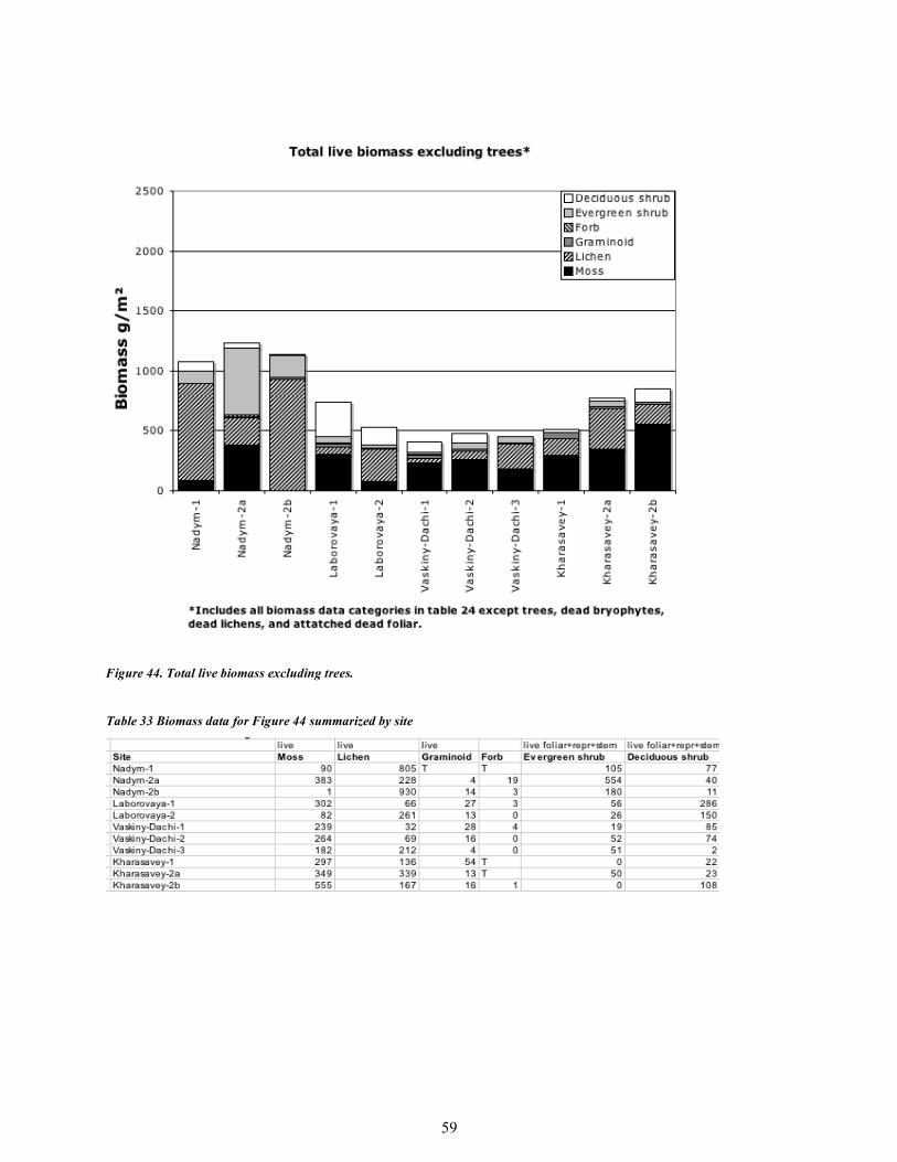
59
Figure 44. Total live biomass excluding trees.
Table 33 Biomass data for Figure 44 summarized by site
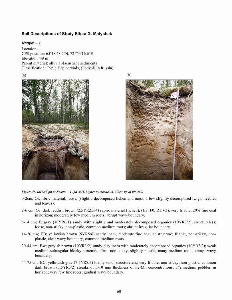
60
Soil Descriptions of Study Sites: G. Matyshak
Nadym – 1 Location: GPS position: 65º18'48.2''N, 72 º53'16.6''E Elevation: 49 m Parent material: alluvial-lacustrine sediments Classification: Typic Haplocryods, (Podzols in Russia)
(a) (b)
Figure 45. (a) Soil pit at Nadym – 1 (pit №1), higher microsite. (b) Close up of pit wall.
0-2cm; Oi; fibric material, loose, (slightly decomposed lichen and moss, a few slightly decomposed twigs, needles and leaves).
2-6 cm; Oa; dark reddish brown (2.5YR2.5/4) sapric material (lichen), (H8, F0, R1,V3), very friable, 20% fine coal in horizon; moderately few medium roots; abrupt wavy boundary.
6-14 cm; Е; gray (10YR6/1) sandy with slightly and moderately decomposed organics (10YR3/2); structureless; loose, non-sticky, non-plastic, common medium roots; abrupt irregular boundary.
14-20 cm; ЕВ; yellowish brown (5YR5/6) sandy loam; moderate fine angular structure; friable, non-sticky, non-plastic, clear wavy boundary, common medium roots.
20-44 cm; Вw; grayish brown (10YR3/2) sandy clay loam with moderately decomposed organics (10YR2/2); weak medium subangular blocky structure; firm, non-sticky, slightly plastic; many medium roots, abrupt wavy boundary.
44-75 cm; ВC; yellowish gray (7.5YR8/3) loamy sand; structureless; very friable, non-sticky, non-plastic, common dark brown (7.5YR3/2) streaks of 5-10 mm thickness of Fe-Mn concentrations; 5% medium pebbles in horizon; very few fine roots; gradual wavy boundary.
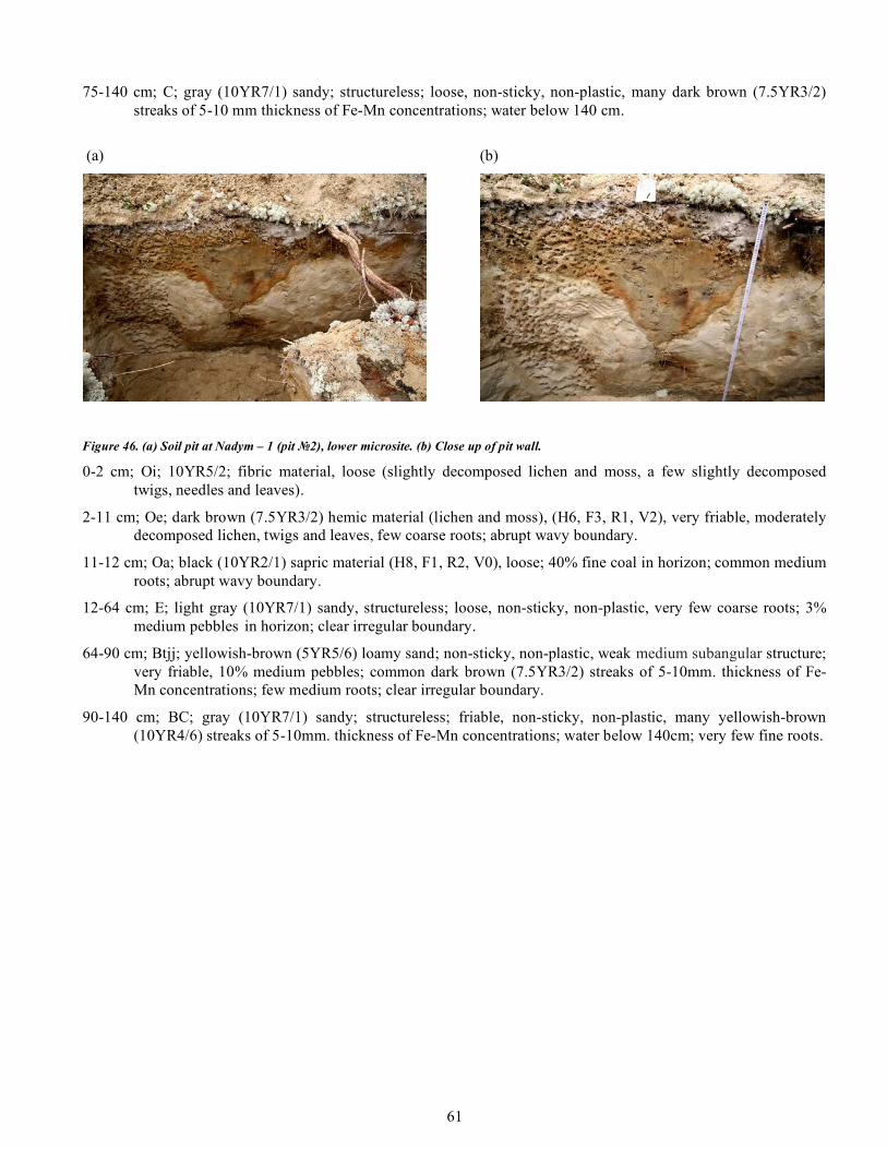
61
75-140 cm; С; gray (10YR7/1) sandy; structureless; loose, non-sticky, non-plastic, many dark brown (7.5YR3/2) streaks of 5-10 mm thickness of Fe-Mn concentrations; water below 140 cm.
(a) (b)
Figure 46. (a) Soil pit at Nadym – 1 (pit №2), lower microsite. (b) Close up of pit wall.
0-2 cm; Oi; 10YR5/2; fibric material, loose (slightly decomposed lichen and moss, a few slightly decomposed twigs, needles and leaves).
2-11 cm; Oe; dark brown (7.5YR3/2) hemic material (lichen and moss), (H6, F3, R1, V2), very friable, moderately decomposed lichen, twigs and leaves, few coarse roots; abrupt wavy boundary.
11-12 cm; Oa; black (10YR2/1) sapric material (H8, F1, R2, V0), loose; 40% fine coal in horizon; common medium roots; abrupt wavy boundary.
12-64 cm; Е; light gray (10YR7/1) sandy, structureless; loose, non-sticky, non-plastic, very few coarse roots; 3% medium pebbles in horizon; clear irregular boundary.
64-90 cm; Вtjj; yellowish-brown (5YR5/6) loamy sand; non-sticky, non-plastic, weak medium subangular structure; very friable, 10% medium pebbles; common dark brown (7.5YR3/2) streaks of 5-10mm. thickness of Fe-Mn concentrations; few medium roots; clear irregular boundary.
90-140 cm; BС; gray (10YR7/1) sandy; structureless; friable, non-sticky, non-plastic, many yellowish-brown (10YR4/6) streaks of 5-10mm. thickness of Fe-Mn concentrations; water below 140cm; very few fine roots.
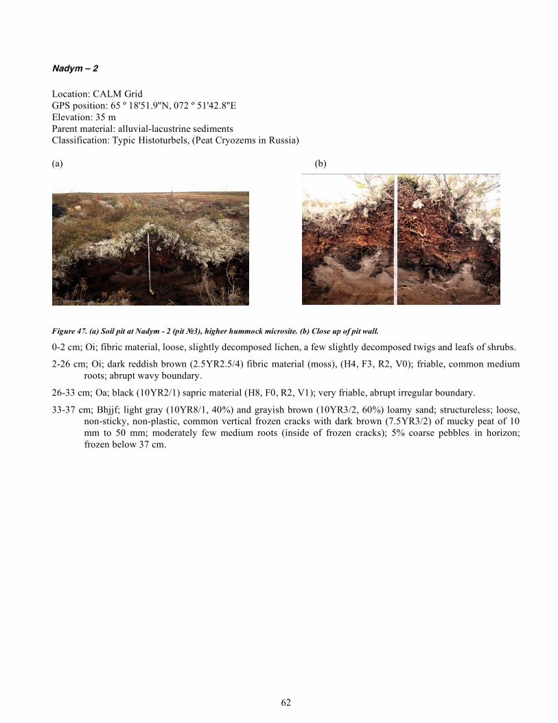
62
Nadym – 2 Location: CALM Grid GPS position: 65 º 18'51.9''N, 072 º 51'42.8''E Elevation: 35 m Parent material: alluvial-lacustrine sediments Classification: Typic Histoturbels, (Peat Cryozems in Russia) (a) (b)
Figure 47. (a) Soil pit at Nadym - 2 (pit №3), higher hummock microsite. (b) Close up of pit wall.
0-2 cm; Oi; fibric material, loose, slightly decomposed lichen, a few slightly decomposed twigs and leafs of shrubs.
2-26 cm; Oi; dark reddish brown (2.5YR2.5/4) fibric material (moss), (H4, F3, R2, V0); friable, common medium roots; abrupt wavy boundary.
26-33 cm; Oa; black (10YR2/1) sapric material (H8, F0, R2, V1); very friable, abrupt irregular boundary.
33-37 cm; Вhjjf; light gray (10YR8/1, 40%) and grayish brown (10YR3/2, 60%) loamy sand; structureless; loose, non-sticky, non-plastic, common vertical frozen cracks with dark brown (7.5YR3/2) of mucky peat of 10 mm to 50 mm; moderately few medium roots (inside of frozen cracks); 5% coarse pebbles in horizon; frozen below 37 cm.
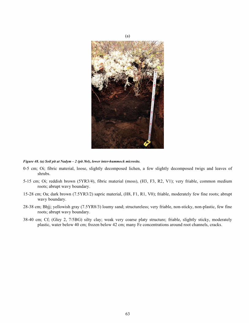
63
(a)
Figure 48. (a) Soil pit at Nadym – 2 (pit №4), lower inter-hummock microsite.
0-5 cm; Oi; fibric material, loose, slightly decomposed lichen, a few slightly decomposed twigs and leaves of shrubs.
5-15 cm; Oi; reddish brown (5YR3/4), fibric material (moss), (H3, F3, R2, V1); very friable, common medium roots; abrupt wavy boundary.
15-28 cm; Oa; dark brown (7.5YR3/2) sapric material, (H8, F1, R1, V0); friable, moderately few fine roots; abrupt wavy boundary.
28-38 cm; Вhjj; yellowish gray (7.5YR8/3) loamy sand; structureless; very friable, non-sticky, non-plastic, few fine roots; abrupt wavy boundary.
38-40 cm; Cf; (Gley 2, 7/5BG) silty clay; weak very coarse platy structure; friable, slightly sticky, moderately plastic, water below 40 cm; frozen below 42 cm; many Fe concentrations around root channels, cracks.
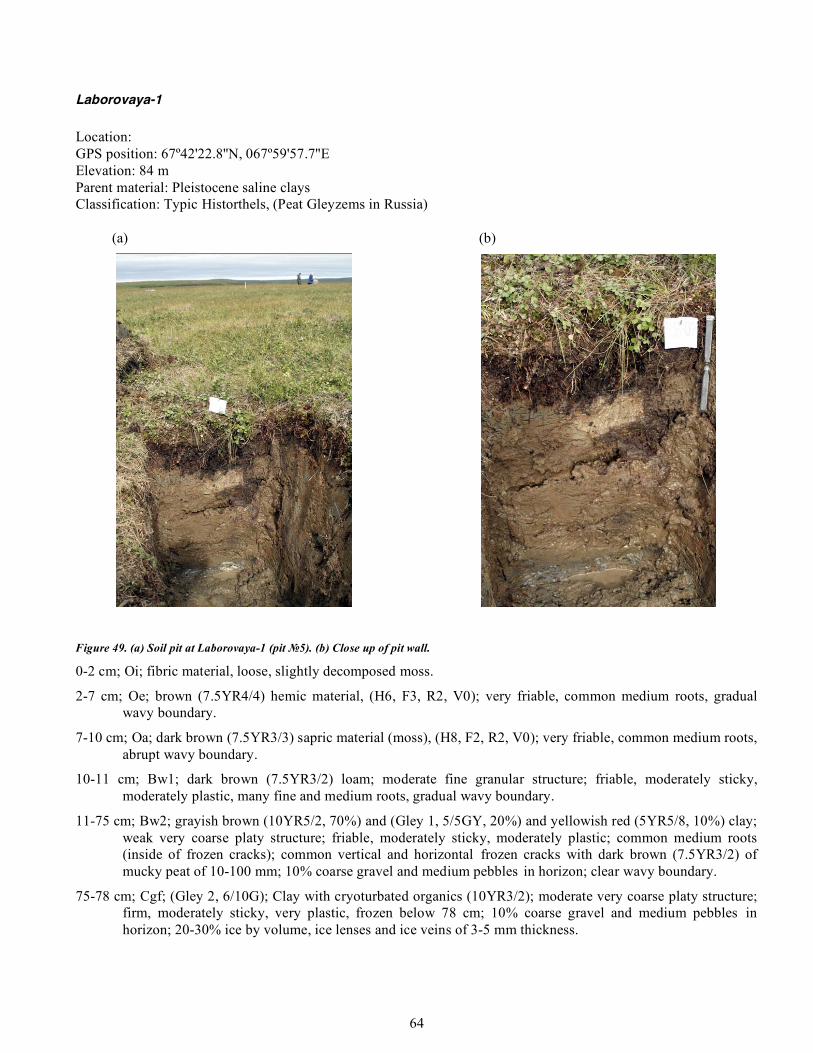
64
Laborovaya-1 Location: GPS position: 67º42'22.8''N, 067º59'57.7''E Elevation: 84 m Parent material: Pleistocene saline clays Classification: Typic Historthels, (Peat Gleyzems in Russia) (a) (b)
Figure 49. (a) Soil pit at Laborovaya-1 (pit №5). (b) Close up of pit wall.
0-2 cm; Oi; fibric material, loose, slightly decomposed moss.
2-7 cm; Oe; brown (7.5YR4/4) hemic material, (H6, F3, R2, V0); very friable, common medium roots, gradual wavy boundary.
7-10 cm; Oa; dark brown (7.5YR3/3) sapric material (moss), (H8, F2, R2, V0); very friable, common medium roots, abrupt wavy boundary.
10-11 cm; Bw1; dark brown (7.5YR3/2) loam; moderate fine granular structure; friable, moderately sticky, moderately plastic, many fine and medium roots, gradual wavy boundary.
11-75 cm; Bw2; grayish brown (10YR5/2, 70%) and (Gley 1, 5/5GY, 20%) and yellowish red (5YR5/8, 10%) clay; weak very coarse platy structure; friable, moderately sticky, moderately plastic; common medium roots (inside of frozen cracks); common vertical and horizontal frozen cracks with dark brown (7.5YR3/2) of mucky peat of 10-100 mm; 10% coarse gravel and medium pebbles in horizon; clear wavy boundary.
75-78 cm; Cgf; (Gley 2, 6/10G); Clay with cryoturbated organics (10YR3/2); moderate very coarse platy structure; firm, moderately sticky, very plastic, frozen below 78 cm; 10% coarse gravel and medium pebbles in horizon; 20-30% ice by volume, ice lenses and ice veins of 3-5 mm thickness.
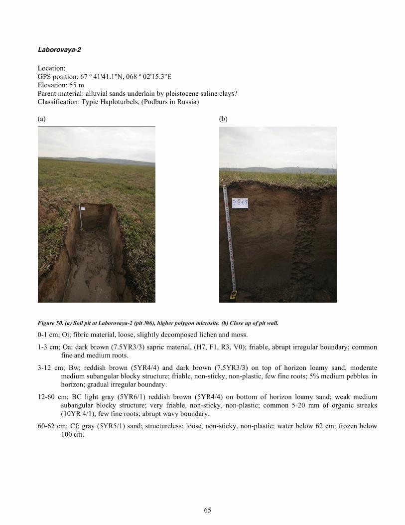
65
Laborovaya-2 Location: GPS position: 67 º 41'41.1''N, 068 º 02'15.3''E Elevation: 55 m Parent material: alluvial sands underlain by pleistocene saline clays? Classification: Typic Haploturbels, (Podburs in Russia) (a) (b)
Figure 50. (a) Soil pit at Laborovaya-2 (pit №6), higher polygon microsite. (b) Close up of pit wall.
0-1 cm; Oi; fibric material, loose, slightly decomposed lichen and moss.
1-3 cm; Oa; dark brown (7.5YR3/3) sapric material, (H7, F1, R3, V0); friable, abrupt irregular boundary; common fine and medium roots.
3-12 cm; Вw; reddish brown (5YR4/4) and dark brown (7.5YR3/3) on top of horizon loamy sand, moderate medium subangular blocky structure; friable, non-sticky, non-plastic, few fine roots; 5% medium pebbles in horizon; gradual irregular boundary.
12-60 cm; ВC light gray (5YR6/1) reddish brown (5YR4/4) on bottom of horizon loamy sand; weak medium subangular blocky structure; very friable, non-sticky, non-plastic; common 5-20 mm of organic streaks (10YR 4/1), few fine roots; abrupt wavy boundary.
60-62 cm; Сf; gray (5YR5/1) sand; structureless; loose, non-sticky, non-plastic; water below 62 cm; frozen below 100 cm.
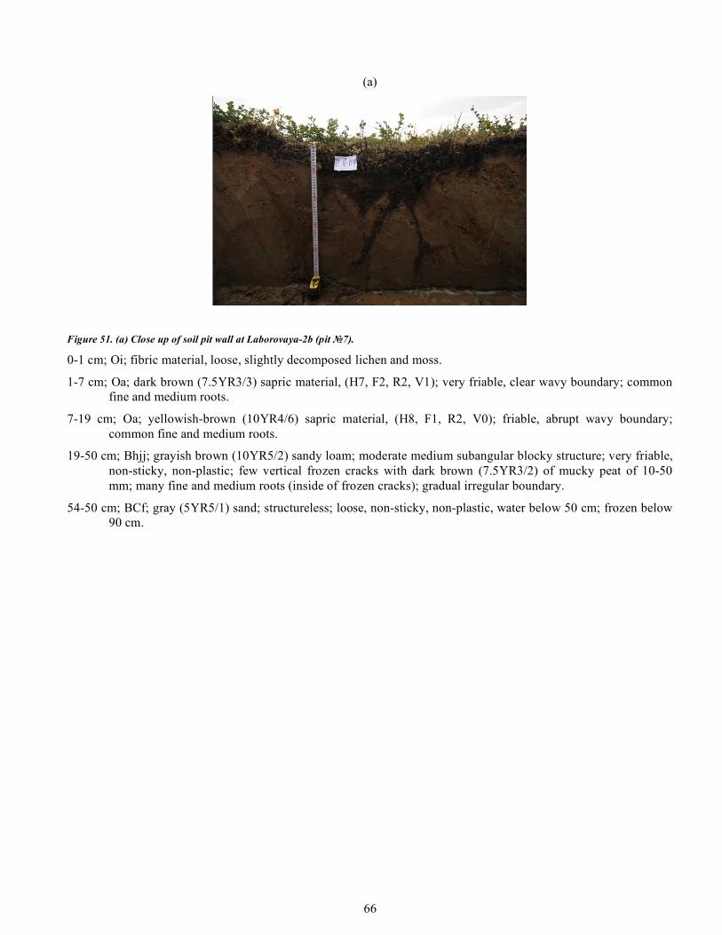
66
(a)
Figure 51. (a) Close up of soil pit wall at Laborovaya-2b (pit №7).
0-1 cm; Oi; fibric material, loose, slightly decomposed lichen and moss.
1-7 cm; Oa; dark brown (7.5YR3/3) sapric material, (H7, F2, R2, V1); very friable, clear wavy boundary; common fine and medium roots.
7-19 cm; Oa; yellowish-brown (10YR4/6) sapric material, (H8, F1, R2, V0); friable, abrupt wavy boundary; common fine and medium roots.
19-50 cm; Вhjj; grayish brown (10YR5/2) sandy loam; moderate medium subangular blocky structure; very friable, non-sticky, non-plastic; few vertical frozen cracks with dark brown (7.5YR3/2) of mucky peat of 10-50 mm; many fine and medium roots (inside of frozen cracks); gradual irregular boundary.
54-50 cm; BСf; gray (5YR5/1) sand; structureless; loose, non-sticky, non-plastic, water below 50 cm; frozen below 90 cm.
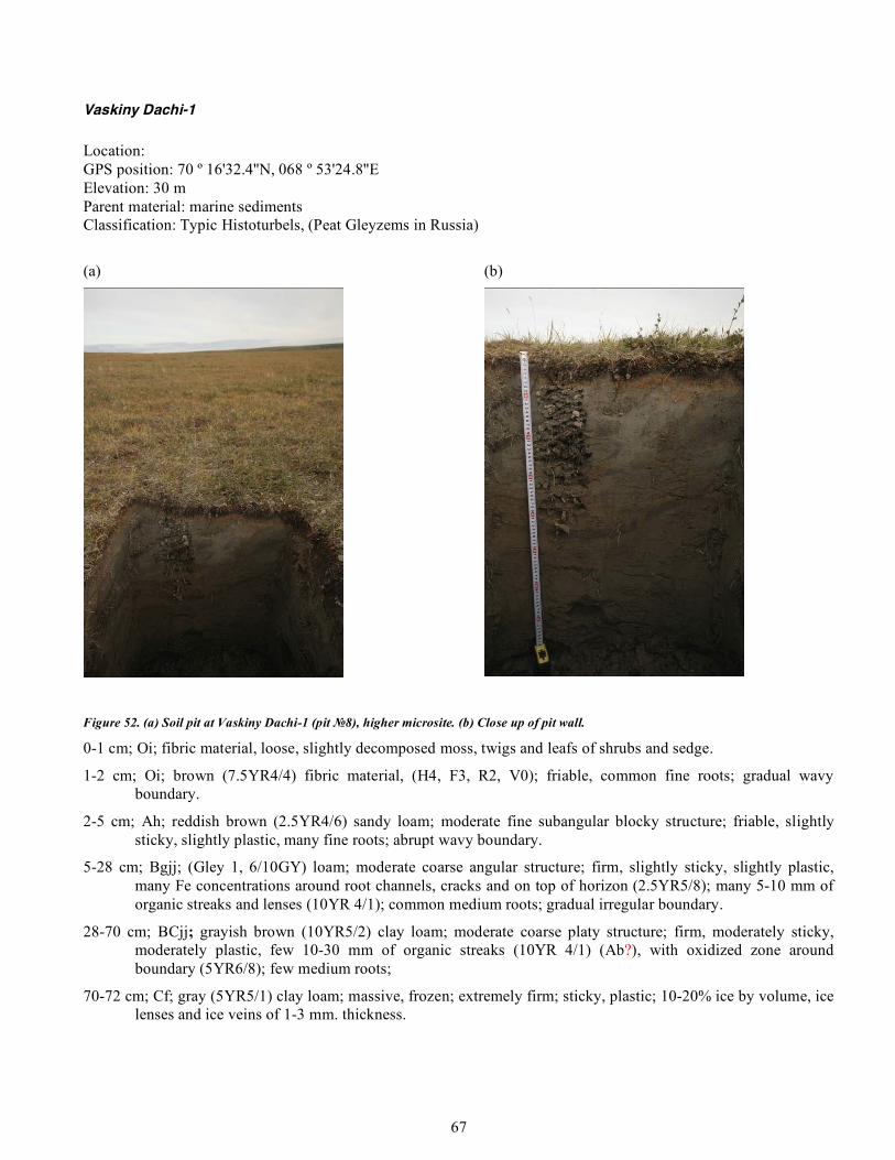
67
Vaskiny Dachi-1 Location: GPS position: 70 º 16'32.4''N, 068 º 53'24.8''E Elevation: 30 m Parent material: marine sediments Classification: Typic Histoturbels, (Peat Gleyzems in Russia)
(a) (b)
Figure 52. (a) Soil pit at Vaskiny Dachi-1 (pit №8), higher microsite. (b) Close up of pit wall.
0-1 cm; Oi; fibric material, loose, slightly decomposed moss, twigs and leafs of shrubs and sedge.
1-2 cm; Oi; brown (7.5YR4/4) fibric material, (H4, F3, R2, V0); friable, common fine roots; gradual wavy boundary.
2-5 cm; Аh; reddish brown (2.5YR4/6) sandy loam; moderate fine subangular blocky structure; friable, slightly sticky, slightly plastic, many fine roots; abrupt wavy boundary.
5-28 cm; Bgjj; (Gley 1, 6/10GY) loam; moderate coarse angular structure; firm, slightly sticky, slightly plastic, many Fe concentrations around root channels, cracks and on top of horizon (2.5YR5/8); many 5-10 mm of organic streaks and lenses (10YR 4/1); common medium roots; gradual irregular boundary.
28-70 cm; BСjj; grayish brown (10YR5/2) clay loam; moderate coarse platy structure; firm, moderately sticky, moderately plastic, few 10-30 mm of organic streaks (10YR 4/1) (Ab?), with oxidized zone around boundary (5YR6/8); few medium roots;
70-72 cm; Cf; gray (5YR5/1) clay loam; massive, frozen; extremely firm; sticky, plastic; 10-20% ice by volume, ice lenses and ice veins of 1-3 mm. thickness.
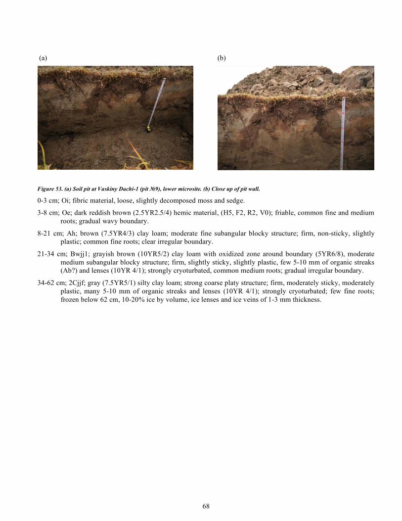
68
(a) (b)
Figure 53. (a) Soil pit at Vaskiny Dachi-1 (pit №9), lower microsite. (b) Close up of pit wall.
0-3 cm; Oi; fibric material, loose, slightly decomposed moss and sedge.
3-8 cm; Oe; dark reddish brown (2.5YR2.5/4) hemic material, (H5, F2, R2, V0); friable, common fine and medium roots; gradual wavy boundary.
8-21 cm; Аh; brown (7.5YR4/3) clay loam; moderate fine subangular blocky structure; firm, non-sticky, slightly plastic; common fine roots; clear irregular boundary.
21-34 cm; Bwjj1; grayish brown (10YR5/2) clay loam with oxidized zone around boundary (5YR6/8), moderate medium subangular blocky structure; firm, slightly sticky, slightly plastic, few 5-10 mm of organic streaks (Ab?) and lenses (10YR 4/1); strongly cryoturbated, common medium roots; gradual irregular boundary.
34-62 cm; 2Cjjf; gray (7.5YR5/1) silty clay loam; strong coarse platy structure; firm, moderately sticky, moderately plastic, many 5-10 mm of organic streaks and lenses (10YR 4/1); strongly cryoturbated; few fine roots; frozen below 62 cm, 10-20% ice by volume, ice lenses and ice veins of 1-3 mm thickness.
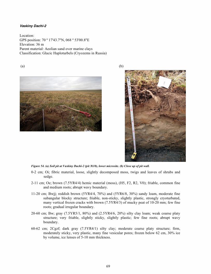
69
Vaskiny Dachi-2 Location: GPS position: 70 º 17'43.7''N, 068 º 53'00.8''E Elevation: 36 m Parent material: Aeolian sand over marine clays Classification: Glacic Haploturbels (Cryozems in Russia)
(a) (b)
Figure 54. (a) Soil pit at Vaskiny Dachi-2 (pit №10), lower microsite. (b) Close up of pit wall.
0-2 cm; Oi; fibric material, loose, slightly decomposed moss, twigs and leaves of shrubs and sedge.
2-11 cm; Oe; brown (7.5YR4/4) hemic material (moss), (H5, F2, R2, V0); friable, common fine and medium roots; abrupt wavy boundary.
11-20 cm; Bwjj; reddish brown (5YR4/4, 70%) and (5YR6/8, 30%) sandy loam, moderate fine subangular blocky structure; friable, non-sticky, slightly plastic, strongly cryoturbated, many vertical frozen cracks with brown (7.5YR4/3) of mucky peat of 10-20 mm; few fine roots; gradual irregular boundary.
20-60 cm; Bw; gray (7.5YR5/1, 80%) and (2.5YR4/6, 20%) silty clay loam; weak coarse platy structure; very friable, slightly sticky, slightly plastic; few fine roots; abrupt wavy boundary.
60-62 cm; 2Cgzf; dark gray (7.5YR4/1) silty clay; moderate coarse platy structure; firm, moderately sticky, very plastic, many fine vesicular pores; frozen below 62 cm, 30% ice by volume, ice lenses of 5-10 mm thickness.
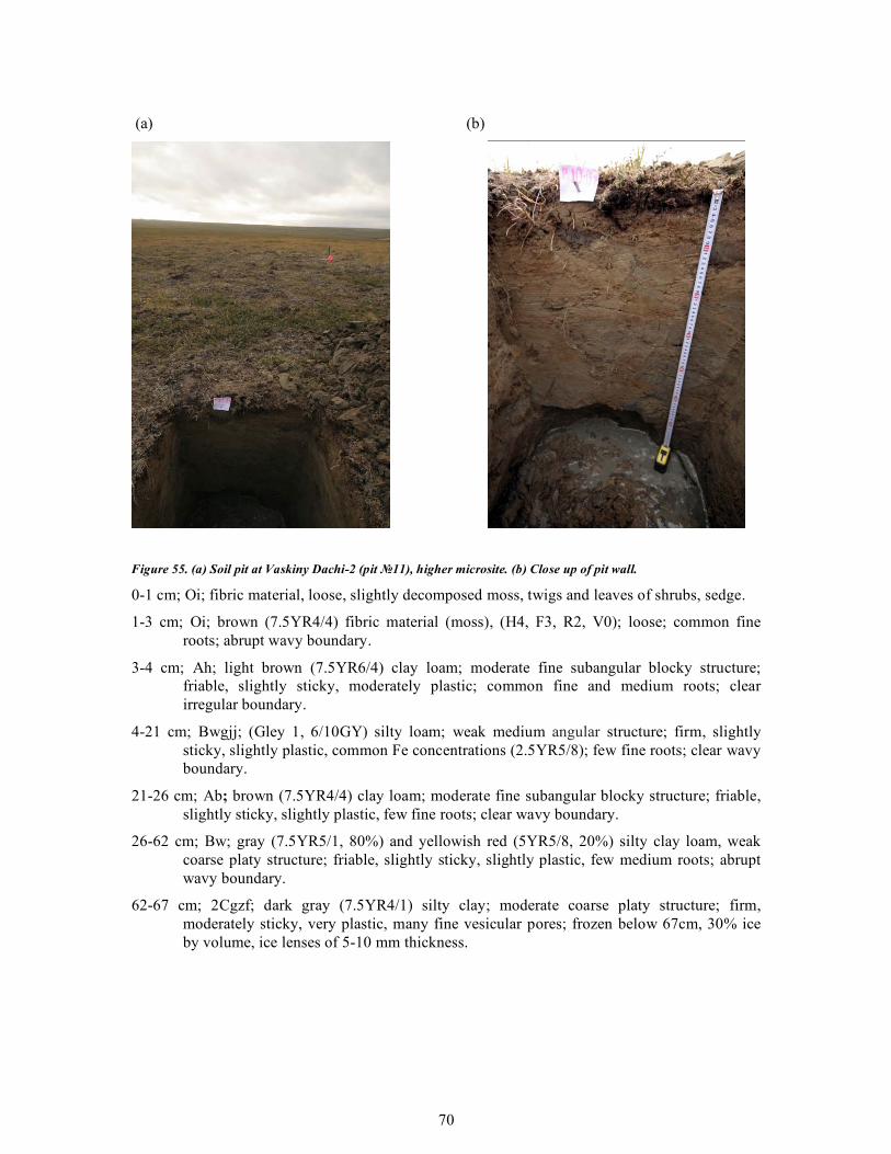
70
(a) (b)
Figure 55. (a) Soil pit at Vaskiny Dachi-2 (pit №11), higher microsite. (b) Close up of pit wall.
0-1 cm; Oi; fibric material, loose, slightly decomposed moss, twigs and leaves of shrubs, sedge.
1-3 cm; Oi; brown (7.5YR4/4) fibric material (moss), (H4, F3, R2, V0); loose; common fine roots; abrupt wavy boundary.
3-4 cm; Аh; light brown (7.5YR6/4) clay loam; moderate fine subangular blocky structure; friable, slightly sticky, moderately plastic; common fine and medium roots; clear irregular boundary.
4-21 cm; Bwgjj; (Gley 1, 6/10GY) silty loam; weak medium angular structure; firm, slightly sticky, slightly plastic, common Fe concentrations (2.5YR5/8); few fine roots; clear wavy boundary.
21-26 cm; Аb; brown (7.5YR4/4) clay loam; moderate fine subangular blocky structure; friable, slightly sticky, slightly plastic, few fine roots; clear wavy boundary.
26-62 cm; Bw; gray (7.5YR5/1, 80%) and yellowish red (5YR5/8, 20%) silty clay loam, weak coarse platy structure; friable, slightly sticky, slightly plastic, few medium roots; abrupt wavy boundary.
62-67 cm; 2Cgzf; dark gray (7.5YR4/1) silty clay; moderate coarse platy structure; firm, moderately sticky, very plastic, many fine vesicular pores; frozen below 67cm, 30% ice by volume, ice lenses of 5-10 mm thickness.
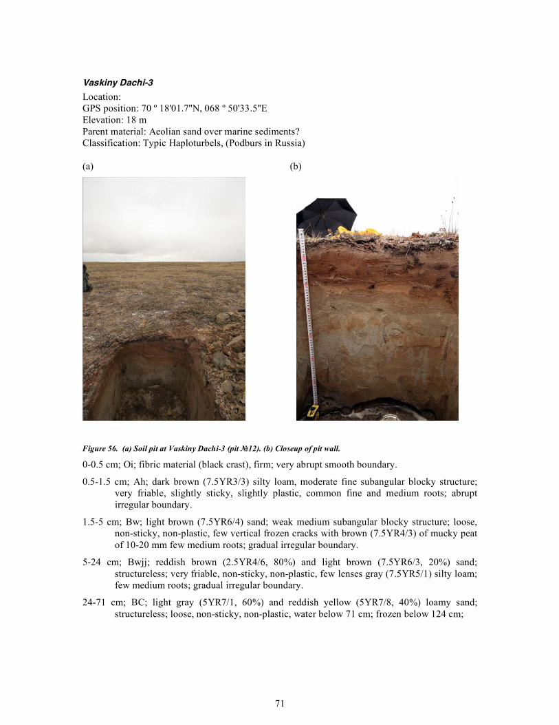
71
Vaskiny Dachi-3 Location: GPS position: 70 º 18'01.7''N, 068 º 50'33.5''E Elevation: 18 m Parent material: Aeolian sand over marine sediments? Classification: Typic Haploturbels, (Podburs in Russia) (a) (b)
Figure 56. (a) Soil pit at Vaskiny Dachi-3 (pit №12). (b) Closeup of pit wall.
0-0.5 cm; Oi; fibric material (black crast), firm; very abrupt smooth boundary.
0.5-1.5 cm; Аh; dark brown (7.5YR3/3) silty loam, moderate fine subangular blocky structure; very friable, slightly sticky, slightly plastic, common fine and medium roots; abrupt irregular boundary.
1.5-5 cm; Bw; light brown (7.5YR6/4) sand; weak medium subangular blocky structure; loose, non-sticky, non-plastic, few vertical frozen cracks with brown (7.5YR4/3) of mucky peat of 10-20 mm few medium roots; gradual irregular boundary.
5-24 cm; Bwjj; reddish brown (2.5YR4/6, 80%) and light brown (7.5YR6/3, 20%) sand; structureless; very friable, non-sticky, non-plastic, few lenses gray (7.5YR5/1) silty loam; few medium roots; gradual irregular boundary.
24-71 cm; BC; light gray (5YR7/1, 60%) and reddish yellow (5YR7/8, 40%) loamy sand; structureless; loose, non-sticky, non-plastic, water below 71 cm; frozen below 124 cm;
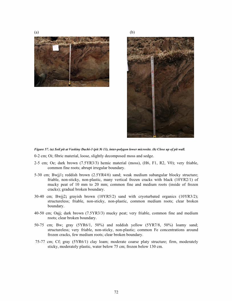
72
(a) (b)
Figure 57. (a) Soil pit at Vaskiny Dachi-3 (pit № 13), inter-polygon lower microsite. (b) Close up of pit wall.
0-2 cm; Oi; fibric material, loose, slightly decomposed moss and sedge.
2-5 cm; Oe; dark brown (7.5YR3/3) hemic material (moss), (H6, F1, R2, V0); very friable, common fine roots; abrupt irregular boundary.
5-30 cm; Bwjj1; reddish brown (2.5YR4/6) sand; weak medium subangular blocky structure; friable, non-sticky, non-plastic, many vertical frozen cracks with black (10YR2/1) of mucky peat of 10 mm to 20 mm; common fine and medium roots (inside of frozen cracks); gradual broken boundary.
30-40 cm; Bwjj2; grayish brown (10YR5/2) sand with cryoturbated organics (10YR3/2); structureless; friable, non-sticky, non-plastic, common medium roots; clear broken boundary.
40-50 cm; Oajj; dark brown (7.5YR3/3) mucky peat; very friable, common fine and medium roots; clear broken boundary.
50-75 cm; Bw; gray (5YR6/1, 50%) and reddish yellow (5YR7/8, 50%) loamy sand; structureless; very friable, non-sticky, non-plastic; common Fe concentrations around frozen cracks, few medium roots; clear broken boundary.
75-77 cm; Cf; gray (5YR6/1) clay loam; moderate coarse platy structure; firm, moderately sticky, moderately plastic, water below 75 cm; frozen below 130 cm.
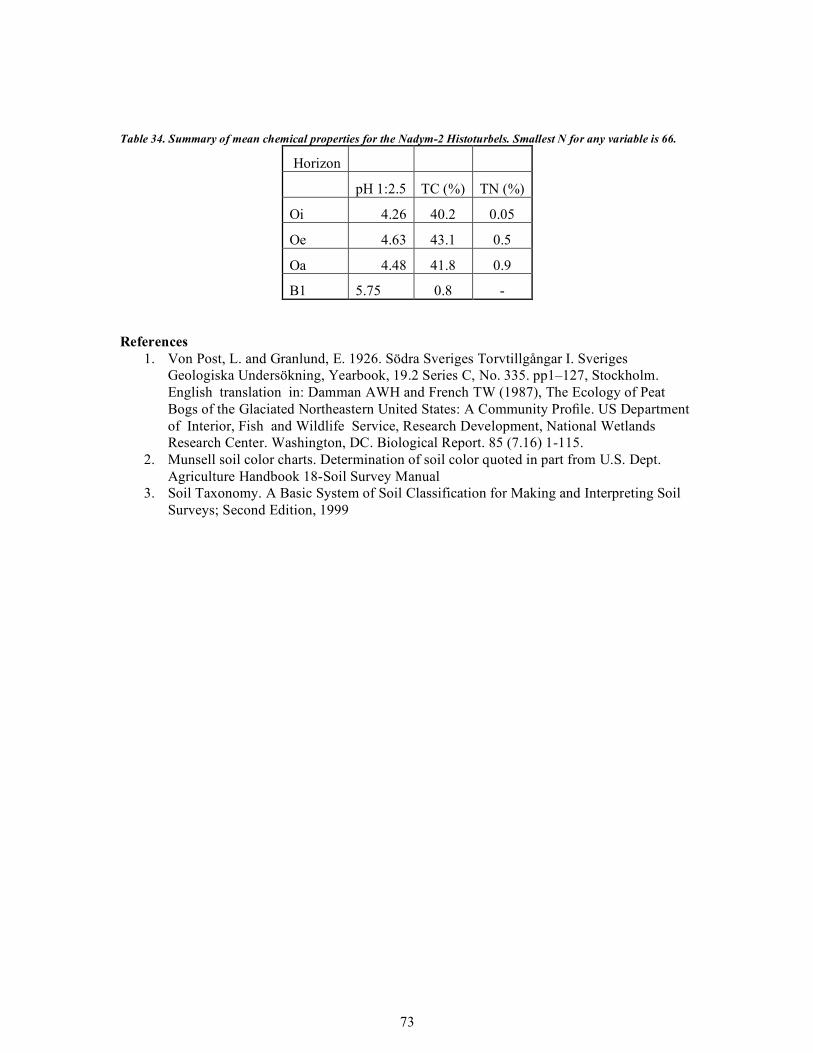
73
Table 34. Summary of mean chemical properties for the Nadym-2 Histoturbels. Smallest N for any variable is 66.
Horizon
pH 1:2.5 TC (%) TN (%)
Oi 4.26 40.2 0.05
Oe 4.63 43.1 0.5
Oa 4.48 41.8 0.9
В1 5.75 0.8 -
References 1. Von Post, L. and Granlund, E. 1926. Södra Sveriges Torvtillgångar I. Sveriges
Geologiska Undersökning, Yearbook, 19.2 Series C, No. 335. pp1–127, Stockholm. English translation in: Damman AWH and French TW (1987), The Ecology of Peat Bogs of the Glaciated Northeastern United States: A Community Profile. US Department of Interior, Fish and Wildlife Service, Research Development, National Wetlands Research Center. Washington, DC. Biological Report. 85 (7.16) 1-115.
2. Munsell soil color charts. Determination of soil color quoted in part from U.S. Dept. Agriculture Handbook 18-Soil Survey Manual
3. Soil Taxonomy. A Basic System of Soil Classification for Making and Interpreting Soil Surveys; Second Edition, 1999
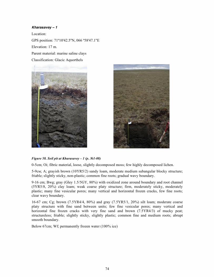
74
Kharasavey – 1
Location:
GPS position: 71º10'42.5''N, 066 º58'47.1''E
Elevation: 17 m.
Parent material: marine saline clays
Classification: Glacic Aquorthels
Figure 58. Soil pit at Kharasavey – 1 (р. №1-08)
0-5cm; Oi; fibric material, loose, slightly decomposed moss; few highly decomposed lichen.
5-9см; A; grayish brown (10YR5/2) sandy loam, moderate medium subangular blocky structure; friable; slightly sticky, non-plastic; common fine roots; gradual wavy boundary.
9-16 cm; Bwg; gray (Gley 1.5/5GY, 80%) with oxidized zone around boundary and root channel (5YR5/8, 20%) clay loam; weak coarse platy structure; firm, moderately sticky, moderately plastic; many fine vesicular pores; many vertical and horizontal frozen cracks, few fine roots; clear wavy boundary.
16-67 cm; Сg; brown (7.5YR4/4, 80%) and gray (7.5YR5/1, 20%) silt loam; moderate coarse platy structure with fine sand between units; few fine vesicular pores; many vertical and horizontal fine frozen cracks with very fine sand and brown (7.5YR4/3) of mucky peat; structureless; friable; slightly sticky, slightly plastic; common fine and medium roots; abrupt smooth boundary.
Below 67cm; Wf; permanently frozen water (100% ice)

75
Kharasavey – 2а
Location:
GPS position: 71º11'39.8''N, 066 º53'20.9''E
Elevation: 2 m.
Parent material: Aeolian (alluvium?) sand over marine saline clays
Classification: Glacic Aquiturbels
Figure 59. Soil pit at Kharasavey – 2a (р. №2-08)
0-4cm; Oi; fibric material, loose, slightly decomposed moss, twigs and leafs of shrubs, sedge.
4-5cm; Oa; reddish brown (5YR3/4), (H7, F1, R2) sapric material (moss); friable; common fine roots; abrupt wavy boundary.
5-9cm; Bw; light brown (7.5YR6/3) sand; structureless; loose; non-sticky, non-plastic; many 0.5-1cm. of organic streaks, dark brown (7.5YR6/3); common fine and medium roots; 1% medium pebbles in horizon; abrupt wavy boundary.
9-19cm; Bwgz; gray (Gley 1.5/5GY) silt loam with oxidized zone around boundary (5YR6/8) and black mottles around root channel (salt?); structureless; firm; slightly sticky, moderately plastic; many fine roots; clear irregular boundary.
19-51cm; Bwjj; yellowish-brown (10YR5/4) sand; structureless; loose; non-sticky, non-plastic; few fine roots; many fine vesicular pores; many medium plants remains; abrupt wavy boundary.
51-62 cm; C; dark gray (7.5YR4/1) silty clay; moderate coarse platy structure; firm; moderately sticky, very plastic; abrupt smooth boundary.
Below 62cm; Wf; permanently frozen water (100% ice)
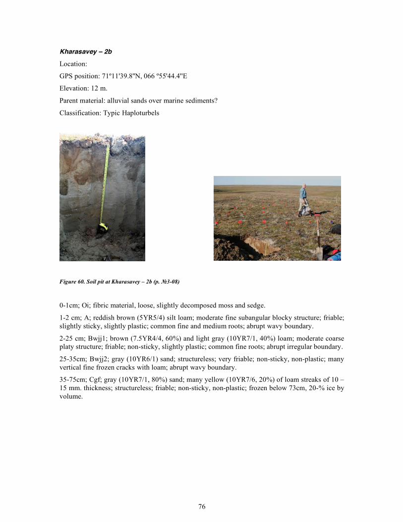
76
Kharasavey – 2b
Location:
GPS position: 71º11'39.8''N, 066 º55'44.4''E
Elevation: 12 m.
Parent material: alluvial sands over marine sediments?
Classification: Typic Haploturbels
Figure 60. Soil pit at Kharasavey – 2b (р. №3-08)
0-1cm; Oi; fibric material, loose, slightly decomposed moss and sedge.
1-2 cm; A; reddish brown (5YR5/4) silt loam; moderate fine subangular blocky structure; friable; slightly sticky, slightly plastic; common fine and medium roots; abrupt wavy boundary.
2-25 cm; Bwjj1; brown (7.5YR4/4, 60%) and light gray (10YR7/1, 40%) loam; moderate coarse platy structure; friable; non-sticky, slightly plastic; common fine roots; abrupt irregular boundary.
25-35cm; Bwjj2; gray (10YR6/1) sand; structureless; very friable; non-sticky, non-plastic; many vertical fine frozen cracks with loam; abrupt wavy boundary.
35-75cm; Cgf; gray (10YR7/1, 80%) sand; many yellow (10YR7/6, 20%) of loam streaks of 10 – 15 mm. thickness; structureless; friable; non-sticky, non-plastic; frozen below 73cm, 20-% ice by volume.
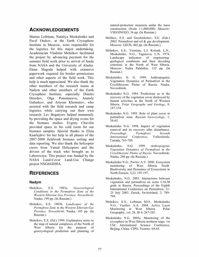
77
ACKNOWLEDGEMENTS Marina Leibman, Nataliya Moskalenko and Pavel Orekov, at the Earth Cryosphere Institute in Moscow, were responsible for the logistics for this major undertaking. Academician Vladimir Melnikov facilitated the project by advancing payment for the summer field work prior to arrival of funds from NASA and the University of Alaska. Elena Slagoda helped with extensive paperwork required for border permissions and other aspects of the field work. This help is much appreciated. We also thank the other members of the research teams at Nadym and other members of the Earth Cryosphere Institute, especially Dimitri Drozdov, Olga Ponomareva, Anatoly Gubarkov, and Artyom Khomutov, who assisted with the field research and camp logistics while carrying out their own research. Lev Bogatyrev helped immensely by providing the space and drying ovens for the biomass studies. Evgeny Chuvilin provided space in his cold room for our biomass samples. Special thanks to Elina Kaarlejärvi for her help in all phases of the 2007-2008 fieldwork biomass sorting and data reporting. We also thank the helicopter crews from Yamal Helicopters and the drivers of the truck who brought us to Laborovaya. This project was funded by the NASA Land-Cover Land-Use Change project NNG6GE00A.
REFERENCES Nadym Melnikov, E.S. 1983a. Geocryological
Conditions in the Permafrost Zone of the Western Siberian Gas Province. Novosibirsk: Nauka, 199 pp. (In Russian.)
Melnikov, E.S. 1983b. Landscapes of the Permafrost Zone in the Western Siberian Gas Province. Novosibirsk: Nauka, 185 pp. (In Russian.)
Melnikov, E.S. (Ed.) 1999. Explanatory notes to the map of natural complexes of the North of West Siberia for the purpose of geocryological prediction and planning of
natural-protection measures under the mass construction. (Scale 1:1,000,000). Moscow: VSEGINGEO, 36 pp. (In Russian.)
Melikov, E.S. and Grechishchev, S.E. (Eds.) 2002. Permafrost and oil & gas development. Moscow: GEOS, 402 pp. (In Russian.)
Melnikov, E.S., Veisman, L.I. Kritsuk, L.N., Moskalenko, N.G., Tagunova, L.N. 1974. Landscape indicators of engineering-geological conditions and their decoding criterions in the North of West Siberia. Moscow: Nedra Publisher, 132 pp. (In Russian.)
Moskalenko, N. G. 1999. Anthropogenic Vegetation Dynamics of Permafrost in the Cryolithozone Plains of Russia. Nauka, Novosibirsk.
Moskalenko N.G. 1984. Predictions as to the recovery of the vegetation cover destroyed by human activities in the North of Western Siberia. Polar Geography and Geology, 8: 147-154.
Moskalenko N.G. 1995. Role of plant cover in permafrost zone. Russian Geocryology, 1: 58-65.
Moskalenko N.G. 1998. Impact of vegetation removal and its recovery after disturbance. Proceedings Permafrost Seventh International Conference, Yellowknife, Canada, 763-769.
Moskalenko, N.G. 1999. Anthropogenic Vegetation Dynamics of Permafrost in the Cryolithozone Plains of Russia. Novosibirsk: Nauka, 280 pp. (In Russian.)
Moskalenko N.G., Pavlov A.V. 2000. Ecosystem monitoring of West Siberia North. Biodiversity and Dynamics of Ecosystems in North Eurasia, 1(2): 195-197.
Moskalenko, N.G. 2003. Interactions between vegetation and permafrost on some CALM grids in Russia. Proceedings of the Eighth International Conference on Permafrost, 21-25 July 2003, Zurich, Switzerland, 2: 789-794.
Melnikov, E.S., Leibman M.O., Moskalenko N.G., Vasiliev A.A. 2004. Active Layer Monitoring in West Siberia Polar Geography, vol. 28, № 4: 267-285.
Moskalenko N.G. 2005a. Monitoring of the cryosphere in West Siberia northern taiga. 1st CliC International Science Conference, Beijing, China. CIPO, Tromso: 64-65.
78
Moskalenko N.G. 2005b. Permafrost temperature regime of northern taiga landscapes in West Siberia. 2nd European Conference on Permafrost. Abstracts. Potsdam, Terra Nostra, Germany: 138-139.
Moskalenko, N.G. (ed.) 2006. Anthropogenic Changes of Ecosystems in West Siberian Gas Province. Moscow: RASHN, 358 pp. (In Russian).
Moskalenko N. Impact of climate changes on West Siberia northern taiga ecosystems. Proceedings of the VIII International Symposium on Cold Region Development. Tampere, Finland September 25-27, 2007: 98-99.
Pavlov, A.V., Moskalenko, N.G. 2002. The thermal regime of soils in the North of Western Siberia. Permafrost and Periglacial Processes, 13: 43-51.
Ponomareva, O.E. 2005. Monitoring the frost mound surface dynamics along a gas pipeline route Nadym-Punga, northern taiga zone of West Siberia. 2nd European Conference on Permafrost. Abstracts. Potsdam, Germany, 12-16 June: 190.
Ponomareva O. 2007. Impact of climate change on dynamics of processes in West Siberia. Proceedings of the VIII International Symposium on Cold Region Development. Tampere, Finland September 25-27: 99-100.
Laborovaya Bliss, L. C., and N. V. Mateveyeva. 1992.
Circumpolar arctic vegetation. Pages 59-89 in F. S. Chapin III, J. F. Reynolds, G. R. Shaver, and J. Svoboda, editors. Arctic ecosystems in a changing climate: an ecophysiological perspective. Academic Press, New York.
Botch, M. C., T. V. Gerasimenko, and Y. C. Tolchelnikov. 1971. Mires of the Yamal Peninsula. Botanchiski Zhurnal:1421-1434.
CAVM Team, D.A.Walker, W. A. Gould, L. C. Bliss, S. A. Edlund, M. K. Raynolds, S. C. Zoltai, F. J. A. Daniëls, C. Bay, M. Wilhelm, E. Einarsson, G. Gudjonsson, A. Elvebakk, B. E. Johansen, G. V. Ananjeva, D. S. Drozdov, A. E. Katenin, S. S. Kholod, L. A. Konchenko, Y. V. Korostelev, E. S. Melnikov, N. G. Moskalenko, A. N. Polezhaev, O. E. Ponomareva, E. B. Pospelova, I. N. Safronova, R. P. Shelkunova, B. A. Yurtsev, M. D. Fleming, C. J. Markon, D. F. Murray, and S. S. Talbot.
2003. Circumpolar Arctic Vegetation Map. Conservation of Arctic Flora and Fauna (CAFF) Map No. 1, U.S. Fish and Wildlife Service, Anchorage, AK.
Forbes, B.C. (1997) Tundra disturbance studies. IV. Species establishment on anthropogenic primary surfaces, Yamal Peninsula, northwest Siberia, Russia. Polar Geography 21:79-100.)
Ilyina, I. S., E. I. Lapshina, V. D. Makhno, L. I. Meltzer, and E. A. Romanova. 1976. Vegetation of the West Siberian Plain, In. 1:1,500,000. in I. S. Ilyina, editor. GUGC, Moscow.
Meltzer, L. I. 1984. Zonal division of tundra vegetation of the West Siberian plain. Pages 7-19 in I. A. V. Belov, editor. Vegetation of western Siberia and its mapping. Akademia Nauk, Novosibirsk.
Vilchek, G. E., and O. Y. Bykova. 1992. The origin of regional ecological problems within the northern Tyumen Oblast, Russia. Arctic and Alpine Research 24:99-107.
Yurtsev, B. A. 1994. Floristic division of the Arctic. Journal of Vegetation Science 5:765-776.
Vaskiny Dachi Leibman, M.O. 1994. Cryogenic landslides and
their interaction with linear constructions on Yamal Peninsula, Russia. In: D.W.Smith and D.C.Sego (eds.) Proc. of the 7th International Cold Regions Engineering Specialty Conference, Edmonton, Alberta, Canada: 865-869.
Leibman, M.O. 1995. Preliminary results of cryogenic landslides study on Yamal Peninsula, Russia. Permafrost and Periglacial Processes, 6: 259-264.
Leibman, M.O. 1998. Active layer depth measurements in marine saline clayey deposits of Yamal Peninsula, Russia: procedure and interpretation of results. Permafrost. Seventh International Conference, June 23-27, 1998, Proceedings, Yellowknife, Canada: 635-639.
Leibman, M.O. 2001. Procedures and results of active-layer measurements in marine saline deposits of Central Yamal. Earth Cryosphere V(3): 17-24
Leibman, M.O., Archegova, I.B., Gorlanova, L.A., Kizyakov, A.I. 2000. Stages of cryogenic landslides on Yugorsky and Yamal
79
Peninsulas. Earth Cryosphere, IV(4): 67-75 (In Russian).
Leibman, M.O., Egorov, I.P., (1996) Climatic and environmental controls of cryogenic landslides, Yamal, Russia. Landslides. Balkema Publishers, Rotterdam: 1941-1946.
Leibman, M.O., Kizyakov, A.I., Sulerzhitsky, L.D., Zaretskaya, N.E. 2003. Dynamics of the landslide slopes and mechanism of their development on Yamal peninsula, Russia. Proceedings of the International Conference on Permafrost, Zurich 21-25 July 2003. A.A.Balkema Publishers, Rotterdam, Netherlands I: 651-656.
Leibman, M.O., Lakhtina, O.V. , Miklyaev, S.M., Titova, I.R.. 1991. Peculiarities of cryogenic processes expansion and their role in relief formation at the Western Yamal. In: Denudation in Permafrost Zone. Moscow: Nauka, 92-99 (in Russian).
Leibman, M.O., Rivkin, F.M. & Saveliev, V.S. 1993a. Hydrogeological aspects of cryogenic slides on the Yamal Peninsula. International Permafrost Conference, Sixth, Beijing. Proceedings 1: 380-382.
Leibman, M.O., Rivkin, F.M., and Streletskaya, I.D. 1993b. Chemical and physical features of the active layer as related to landslides on Yamal Peninsula. Joint Russian-American Seminar on Cryopedology and Global Change, Pushchino, 1992. Post-Seminar Proceedings: 257-262.
Leibman, M.O., Streletskaya, I.D. 1996. Migration of chemical elements and ions in the active layer and upper part of permafrost in connection with thermodenudation processes on Yamal Peninsula. Proc. of the First conference of Russian geocryologists, book 2. Moscow: Faculty of Geology MSU: 390 -398 (In Russian).
Leibman, M.O., Streletskaya, I.D. 1997. Land-slide induced changes in the chemical composition of active layer soils and surface-water run-off, Yamal Peninsula, Russia. I.K.Iskandar, E.A.Wright, J.K.Radke, B.S.Sharratt, P.H.Groenevelt, and L.D.Hinzman (eds.) Proc.of the International Symposium on Physics, Chemistry, and Ecology of Seasonally Frozen Soils, Fairbanks, Alaska, June 10-12, 1997, CRREL Special Report 97-10, CRREL, Hanover: 120-126.
Leibman, M.O., Streletskaya, I.D., Konyakhin, M.A. 1997. Estimation of the dynamics of
the surface at Bovanenkovo gas field (Central Yamal) during the period 1949-1990. Geomorphologia, 2: 45-48 (In Russian).
Romanovskii, N.N., Gravis G.F., Melnikov E.S., Leibman M.O. (1996) Periglacial processes as geoindicators in the cryolithozone. In: A.R.Berger, W.J.Iams (eds.). Geoindicators. Assessing rapid environmental changes in earth systems. A.A.Balkema publisher, Rotterdam: 47-68.
Streletskii D.A., Streletskaya I.D., Rogov V.V. & Leibman M.O. 2003. Redistribution of ions within the active layer and upper permafrost, Yamal, Russia. In: M.Phillips, S.M. Springman, L.U. Arenson (Eds.) Permafrost: Proсeedings of the 8th Intern. Conference on Permafrost, Zurich, Switzerland, 20-25 July 2003. A.A. Balkema Publishers, 2, 1117-1122.
Ukraintseva, N.G. & Leibman, M.O. & Sreletskaya, I.D. 2000. Peculiarities of landslide process in saline frozen deposits of central Yamal, Russia. In: E. BROMHEAD, N. DIXON AND L-L IBSEN (eds), Landslides. Proc. VIII International Symposium on Landslides 3, London: Thomas Telford, 1495-1500.
Ukraintseva, N.G. & Streletskaya, I.D. 1999. Landscape indication of surface soil on West Yamal landslide slopes. In K.N. Dyakonov, I.I. Mamai (eds.), Lomonosov Moscow State University Landscape School: Traditions, Achievements, Future, 120-129. Moscow: RUSAKI (In Russian).
Ukraintseva, N.G. 1997. Willows tundra of Yamal as the indicator of salinity of superficial sediments. Results of basic research of Earth cryosphere in Arctic and Subarctic. Novosibirsk: Nauka Publisher, 182-187 (in Russian).
Ukraintseva, N.G., 1998. Distribution of shrub tundra on Yamal. Biogeography, materials of Moscow Center of Russian Geographical Society, Moscow, RGO Publisher, v.7, 46-53 (in Russian).
Ukraintseva, N.G., Leibman, M.O. 2000. Productivity of willow-shrub tundra in connection with landslide activity. In: '30th Arctic Workshop', INSTAAR, University of Colorado, Boulder, CO USA, March 15-19 2000, 150-152.
Ukraintseva, N.G., Leibman, M.O. 2007. The effect of cryogenic landslides (active-layer detachments) on fertility of tundra soils on
80
Yamal peninsula, Russia. In: V.Schaefer, R.Schuster & A.Turner (eds.) Conference Presentations: 1st North American Landslide Conference, June 3-8, 2007, Vail, Colorado. Association of Environmental & Engineering Geologists. Omnipress: 1605-1615.
Ukraintseva, N.G., Leibman, M.O., Streletskaya, I.D., Yermokhina, K.A., Smetanin, N.N. 2002. Monitoring of the landslide on saline frozen deposits in typical tundra subzone (Yamal, Bovanenkovo Gas-field area). Proc. of the International conference Ecology of northern teritories of Russia. Problems, prediction of situation, ways of development, solutions. Arkhangelsk, 17 - 22 June 2002,in 2 books, book 1: 832-837. Arkhangelsk: Institute of ecology of the North UrB RAS.
Ukraintseva, N.G., Streletskaya, I.D., Ermokhina, K.A. & Yermakov, S.Yu. 2003. Geochemical properties of plant-soil-permafrost system at landslide slopes, Yamal, Russia. Proceedings of the International Conference on Permafrost, Zurich 21-25 July 2003. A.A.Balkema Publishers, Rotterdam, Netherlands II: 1149-1154.
Kharasavey See page 12.
Soil Descriptions Von Post, L. and Granlund, E. 1926. Södra
Sveriges Torvtillgångar I. Sveriges Geologiska Undersökning, Yearbook, 19.2 Series C, No. 335. pp1–127, Stockholm. English translation in: Damman AWH and French TW (1987), The Ecology of Peat Bogs of the Glaciated Northeastern United States: A Community Profile. US Department of Interior, Fish and Wildlife Service, Research Development, National Wetlands Research Center. Washington, DC. Biological Report. 85 (7.16) 1-115.
Munsell soil color charts. Determination of soil color quoted in part from U.S. Dept. Agriculture Handbook 18-Soil Survey Manual.
Soil Taxonomy. A Basic System of Soil Classification for Making and Interpreting Soil Surveys; Second Edition, 1999.
Species List Elven et al. 2007: Checklist of the Panarctic
Flora (PAF). Vascular plants. -Draft. University of Oslo.
Ignatov M.S., Afonina O.M., Ignatova E.A. et al. Check-list of mosses of East Europe and North Asia // Arctoa. 2006. Vol. 15. P. 1-130.
Konstantinova N.A., Potemkin A.D. Liverworts of the Russia Arctic: an annotated check-list and bibliography // Arctoa. 1996. Vol. 6. P. 125-150.
Kristinsson, H., Zhurbenko, M. 2006: Panarctic lichen checklist (http://archive.arcticportal.org/276/01/Panarctic_lichen_checklist.pdf)
Biomass Sampling Procedures Epstein, H. E., et al. 2007 submitted. Phytomass
patterns across the full temperature gradient of the arctic tundra, Journal of Geophysical Research - Biogeosciences.
Kade, A., V. E. Romanovsky, and D. A. Walker. 2006. The N-factor of nonsorted circles along a climate gradient in Arctic Alaska. Permafrost and Periglacial Processes 17:279-289.
Walker, D.A., H.E. Epstein, J.G. Jia, A. Balsar, C. Copass, E.J. Edwards, W.A. Gould, J. Holllingsworth, J. Knudson, H. Meier, A. Moody, and M.K. Raynolds. 2003. Phytomass, LAI, and NDVI in northern Alaska: relationships to summer warmth, soil pH, plant functional types and extrapolation to the circumpolar Arctic. Journal of Geophysical Research, 108 (D2):8169, doi:10.1029/2001JD000986.
Walker, D. A., H. E. Epstein, W. A. Gould, C. L. Ping, V. E. Romanovsky, Y. Shur, C. T. Tarnocai, R. P. Daanen, G. Gonzalez, A. N. Kade, A. M. Kelley, W. B. Drantz, P. Kuss, N. V. Matveyeva, G. J. Miochaelson, C. A. Munger, D. J. Nickolsky, R. A. Peterson, M. K. Raynolds, and C. M. Vonlanthen. 2007 submitted. Biocomplexity of small patterned-ground features along the North American Arctic Transect. Journal of Geophysical Research – Biogeosciences.
Tree Biomass Equations Muukkonen, P. & Mäkipää, R. 2006. Biomass
equations for European trees: addendum. Silva Fennica 40(4): 763–773.
Zianis, D., Muukkonen, P., Mäkipää, R. & Mencuccini, M. 2005. Biomass and stem volume equations for tree species in Europe. Silva Fennica Monographs 4. 63 p.
81
Other Methods Papers Barbour, M. G., J. H. Burk, W. D. Pitts, F. S.
Gilliam, and M. W. Schwartz. 1996. Terrestrial Plant Ecology. Addison Wesley Longman, Menlo Park, CA.
Buckner, D. L. 1985. Point-intercept sampling in revegetation studies: maximizing objectivity and repeatability. Pages 110-113 in. ESCO Associates, Inc., paper presented at the American Society for Surface Mining and Reclamation meeting, Denver, CO, October 1985.
Cottam, C., and J. T. Curtis. 1956. The use of distance measures in phytosociologial sampling Ecology 37:451-460.
Mueller-Dombois, L. D., and H. Ellenberg. 1974. Aims and Methods of Vegetation Ecology. John Wiley and Sons, New York.
Shimwell, D. W. 1971. The Description and Classification of Vegetation. University of Washington Press, Seattle.

82
APPENDIX A: LIST OF PARTICIPANTS N: Nadym L: Laborovaya V: Vaskiny Dachi K: Kharasavey Dmitri S. Drozdov: N Earth Cryosphere Institute, SB RAS Vavilov Street 30/6, room 15 119991 Moscow, Russia +7-495-135-98-71 [email protected] Evgeny Elanchev: N Earth Cryosphere Institute, SB RAS Malygin Street 86 625026 Tyumen, Russia [email protected] Howard E. Epstein: N, L, V, K Department of Environmental Sciences University of Virginia P.O. Box 400123 Clark Hall, 211 Charlottesville, VA 22904-4123 Phone: +1 434-924-4308 Fax: +1 434-982-2137 Jozef Geml: K Biology and Wildlife Department University of Alaska Fairbanks PO Box 757000 Fairbanks, Alaska 99775-7000 [email protected] [email protected] Anatoly Gubarkov: L, V, K Tyumen State Oil and Gas University Volodarsky Street 38 625000 Tyumen, Russia [email protected] Elina Kaarlejärvi: N, L, V, K Arctic Centre University of Lapland Box 122 96101 Rovaniemi, Finland
+358-50-560-86-87 [email protected] Artyom Khomutov: L, V, K Earth Cryosphere Institute, SB RAS Malygin Street 86 625026 Tyumen, Russia [email protected] Patrick Kuss: N, L, V Institute of Plant Sciences University of Bern Altenbergrain 21 3013 Bern, Switzerland Phone: +41 31 631 4992 Fax: +41 31 631 4942 [email protected] Marina Leibman: L, V, K Earth Cryosphere Institute, SB RAS Vavilov Street 30/6 119991 Moscow, Russia +7-916-607-83-93 [email protected] George V. Matyshak: N, L, V, K Department of Soil Science Lomonosov Moscow State University Leninskie Gory 119992 Moscow, Russia +7-495-939-39-80 [email protected] Nataliya G. Moskalenko: N, L, V, K Earth Cryosphere Institute, SB RAS Vavilov Street 30/6, room 67 119991 Moscow, Russia +7-499-135-98-71 [email protected] Aleksander Nikitin: N Earth Cryosphere Institute, SB RAS Vavilov Street 30/6 119991 Moscow, Russia [email protected] Olga Opokina: N Earth Cryosphere Institute, SB RAS Malygin Street 86 625026 Tyumen, Russia +7-3452-688-787
83
[email protected] Pavel T. Orekhov: N, K Earth Cryosphere Institute, SB RAS Vavilov Street 30/6, room 67 119991 Moscow, Russia +7-499-135-98-71 [email protected] Olga E. Ponomareva: N Earth Cryosphere Institute, SB RAS Vavilov Street 30/6, room 67 119991 Moscow, Russia +7-499-135-98-71 [email protected]
Vladimir Romanovsky: N Department of Geology and Geophysics University of Alaska Fairbanks P.O. Box 755780 Fairbanks, Alaska 99775-5780 +1-907-474-7459 [email protected]
Donald A. Walker: N, L, V, K Institute of Arctic Biology Alaska Geobotany Center University of Alaska Fairbanks PO Box 757000 Fairbanks, Alaska 99775-7000 Phone: +1 907-474-2460 Fax: +1 907-474-7666 [email protected]
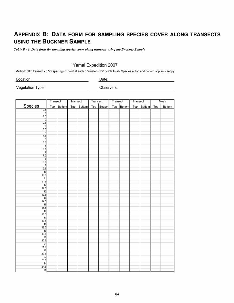
84
APPENDIX B: DATA FORM FOR SAMPLING SPECIES COVER ALONG TRANSECTS USING THE BUCKNER SAMPLE Table B - 1. Data form for sampling species cover along transects using the Buckner Sample
Yamal Expedition 2007
Method: 50m transect - 0.5m spacing - 1 point at each 0.5 meter - 100 points total - Species at top and bottom of plant canopy
Location: Date:
Vegetation Type: Observers:
Transect __ Transect __ Transect __ Transect __ Transect __ Mean
Species Top Bottom Top Bottom Top Bottom Top Bottom Top Bottom Top Bottom0.5
1
1.5
2
2.5
3
3.5
4
4.5
5
5.5
6
6.5
7
7.5
8
8.5
9
9.5
10
10.5
11
11.5
12
12.5
13
13.5
14
14.5
15
15.5
16
16.5
17
17.5
18
18.5
19
19.5
20
20.5
21
21.5
22
22.5
23
23.5
24
24.525

85
APPENDIX C: DATA FORMS FOR RELEVÉ DATA (SITE DESCRIPTION AND SPECIES COVER/ABUNDANCE)
Table C – 1. Relevé data form: Site description, and growth form cover values
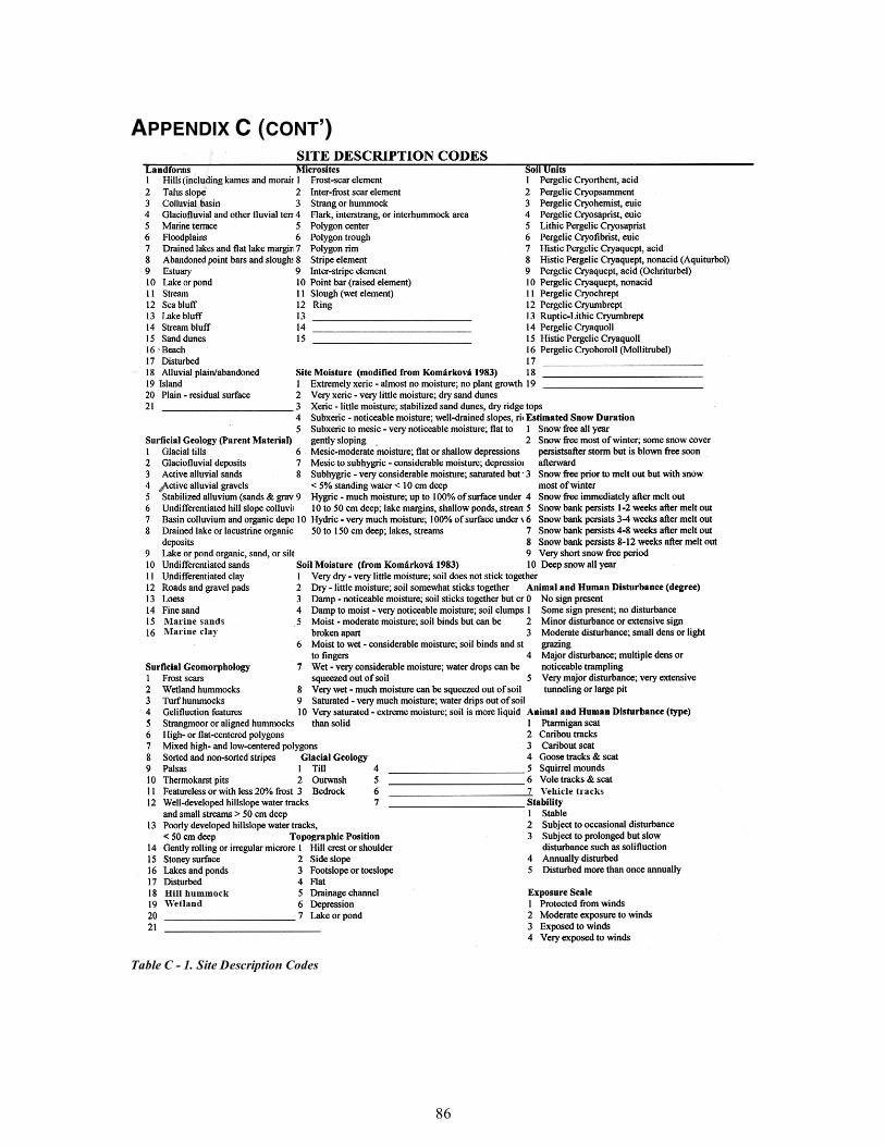
86
APPENDIX C (CONT’)
Table C - 1. Site Description Codes
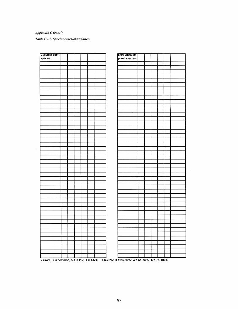
87
Appendix C (cont’)
Table C - 2. Species cover/abundance:
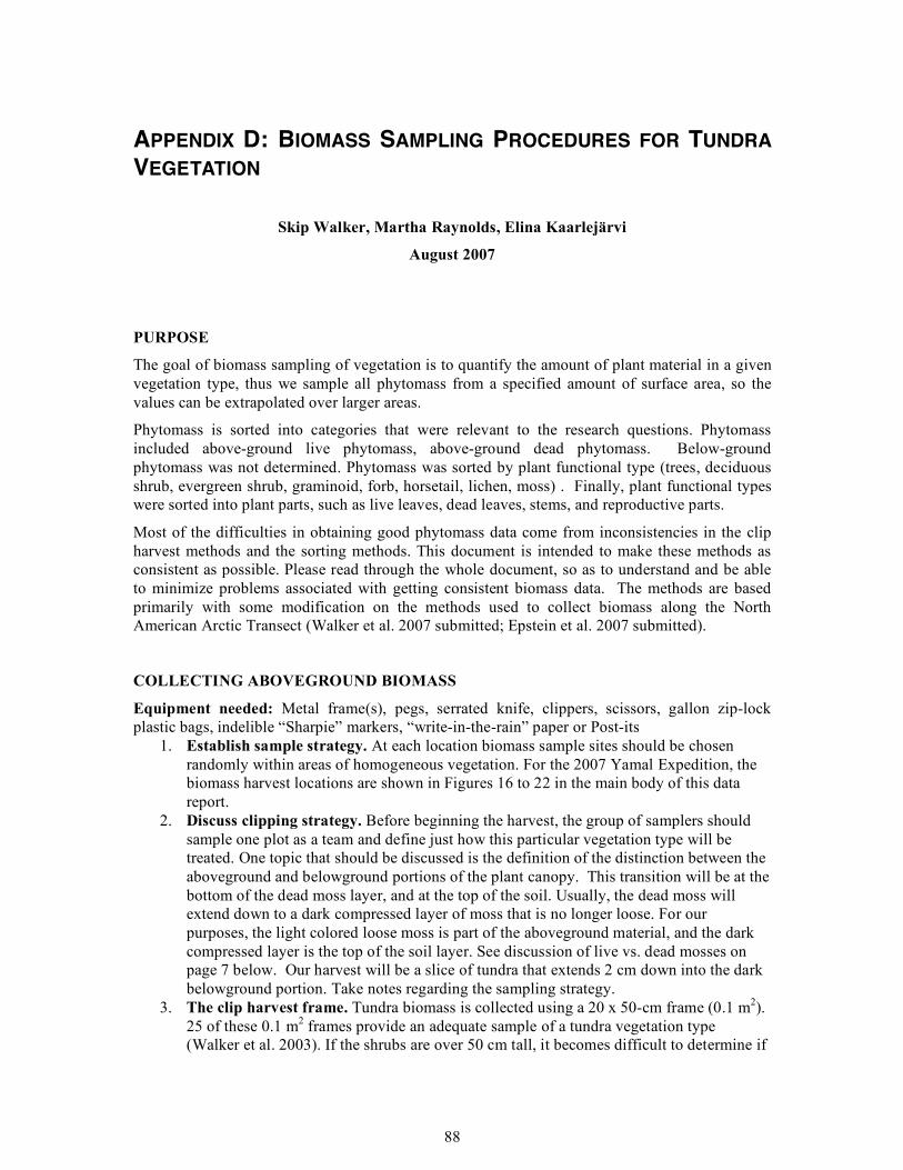
88
APPENDIX D: BIOMASS SAMPLING PROCEDURES FOR TUNDRA VEGETATION
Skip Walker, Martha Raynolds, Elina Kaarlejärvi
August 2007
PURPOSE
The goal of biomass sampling of vegetation is to quantify the amount of plant material in a given vegetation type, thus we sample all phytomass from a specified amount of surface area, so the values can be extrapolated over larger areas.
Phytomass is sorted into categories that were relevant to the research questions. Phytomass included above-ground live phytomass, above-ground dead phytomass. Below-ground phytomass was not determined. Phytomass was sorted by plant functional type (trees, deciduous shrub, evergreen shrub, graminoid, forb, horsetail, lichen, moss) . Finally, plant functional types were sorted into plant parts, such as live leaves, dead leaves, stems, and reproductive parts.
Most of the difficulties in obtaining good phytomass data come from inconsistencies in the clip harvest methods and the sorting methods. This document is intended to make these methods as consistent as possible. Please read through the whole document, so as to understand and be able to minimize problems associated with getting consistent biomass data. The methods are based primarily with some modification on the methods used to collect biomass along the North American Arctic Transect (Walker et al. 2007 submitted; Epstein et al. 2007 submitted).
COLLECTING ABOVEGROUND BIOMASS
Equipment needed: Metal frame(s), pegs, serrated knife, clippers, scissors, gallon zip-lock plastic bags, indelible “Sharpie” markers, “write-in-the-rain” paper or Post-its
1. Establish sample strategy. At each location biomass sample sites should be chosen randomly within areas of homogeneous vegetation. For the 2007 Yamal Expedition, the biomass harvest locations are shown in Figures 16 to 22 in the main body of this data report.
2. Discuss clipping strategy. Before beginning the harvest, the group of samplers should sample one plot as a team and define just how this particular vegetation type will be treated. One topic that should be discussed is the definition of the distinction between the aboveground and belowground portions of the plant canopy. This transition will be at the bottom of the dead moss layer, and at the top of the soil. Usually, the dead moss will extend down to a dark compressed layer of moss that is no longer loose. For our purposes, the light colored loose moss is part of the aboveground material, and the dark compressed layer is the top of the soil layer. See discussion of live vs. dead mosses on page 7 below. Our harvest will be a slice of tundra that extends 2 cm down into the dark belowground portion. Take notes regarding the sampling strategy.
3. The clip harvest frame. Tundra biomass is collected using a 20 x 50-cm frame (0.1 m2). 25 of these 0.1 m2 frames provide an adequate sample of a tundra vegetation type (Walker et al. 2003). If the shrubs are over 50 cm tall, it becomes difficult to determine if
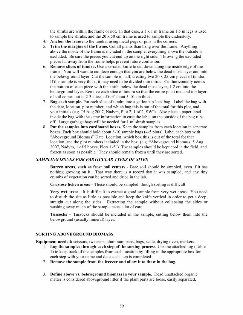
89
the shrubs are within the frame or not. In that case, a 1 x 1 m frame on 1.5 m legs is used to sample the shrubs, and the 20 x 50 cm frame is used to sample the understory.
4. Anchor the frame to the tundra, using metal pegs or pins in the corners. 5. Trim the margins of the frame. Cut all plants than hang over the frame. Anything
above the inside of the frame is included in the sample, everything above the outside is excluded. Be sure the pieces you cut end up on the right side. Throwing the excluded pieces far away from the frame helps prevent future confusion.
6. Remove slices of tundra. Use a serrated knife to cut down along the inside edge of the frame. You will want to cut deep enough that you are below the dead moss layer and into the belowground layer. Cut the sample in half, creating two 20 x 25-cm pieces of tundra. If the sample is very thick, it may need to be divided into thirds. Cut horizontally across the bottom of each piece with the knife, below the dead moss layer, 1-2 cm into the belowground layer. Remove each slice of tundra so that the entire plant mat and top layer of soil comes out in 2-3 slices of turf about 5-10 cm thick.
7. Bag each sample. Put each slice of tundra into a gallon zip-lock bag. Label the bag with the date, location, plot number, and which bag this is out of the total for this plot, and your initials (e.g. “5 Aug 2007, Nadym, Plot 2, 1 of 2, SW”). Also place a paper label inside the bag with the same information in case the label on the outside of the bag rubs off. Large garbage bags will be needed for 1 m2 shrub samples.
8. Put the samples into cardboard boxes. Keep the samples from each location in separate boxes. Each box should hold about 8-10 sample bags (4-5 plots). Label each box with “Aboveground Biomass” Date, Location, which box this is out of the total for that location, and the plot numbers included in the box. (e.g. “Aboveground biomass, 5 Aug 2007, Nadym, 1 of 5 boxes, Plots 1-5”). The samples should be kept cool in the field, and frozen as soon as possible. They should remain frozen until they are sorted.
SAMPLING ISSUES FOR PARTICULAR TYPES OF SITES
Barren areas, such as frost boil centers - Bare soil should be sampled, even if it has nothing growing on it. That way there is a record that it was sampled, and any tiny crumbs of vegetation can be sorted and dried in the lab.
Crustose lichen areas – These should be sampled, though sorting is difficult
Very wet areas - It is difficult to extract a good sample from very wet areas. You need to disturb the site as little as possible and keep the knife vertical in order to get a deep, straight cut along the sides. Extracting the sample without collapsing the sides or washing away much of the sample takes a lot of care.
Tussocks – Tussocks should be included in the sample, cutting below them into the belowground (usually mineral) layer.
SORTING ABOVEGROUND BIOMASS
Equipment needed: scissors, tweezers, aluminum pans, bags, scale, drying oven, markers. 1. Log the samples through each step of the sorting process. Use the attached log (Table
1) to keep track of the samples from each location by filling in the appropriate box for each step with your name and date each step is completed.
2. Remove the sample from the freezer and allow it to thaw in the bag.
3. Define above vs. belowground biomass in your sample. Dead unattached organic
matter is considered aboveground litter if the plant parts are loose, easily separated,

90
distinct and identifiable. Litter that has decomposed beyond this point is considered belowground biomass. Consult any field notes regarding the distinction between above and below ground biomass at this particular location. Remove the belowground biomass from your sample. It should be dried, labeled as “soil and roots” and saved along with the rest of the sample, but there is no need to weigh it.
4. Sorting categories. The sample will be sorted into the following categories: evergreen shrub
stem live foliar attached dead foliar reproductive
deciduous shrub stem live foliar attached dead foliar reproductive
graminoid live attached dead
forb equisetum bryophyte (mosses & liverworts):
live dead
lichen live dead algae litter (all unattached dead plant parts) soil and roots (belowground)
5. Put labels in the sorting tins with the plot number and the above plant categories. 6. Clip with scissors and sort the vascular plants into their specific categories. Cut off
vascular plants above the roots or base of green stems in herbaceous species. This is generally the same location as the above/belowground definition as above, but some plants may have roots in the dead moss layer. Include all attached dead. See below for issues associated with particular species.
7. Sort the lichens, equisetum and algae into their categories. These are usually loose and can be immediately separated. Keep your sample moist or the plants will crumble. If it has dried out, you can always wet it again. If you have a relatively intact moss mat, you may be able to separate litter from moss by turning it upside-down and brushing it gently.
8. Separate the live moss from the dead moss and sort into subcategories if needed. Be aware that many mosses are brown, so the live/dead distinction cannot be done solely on color (see details below)!
9. Sort the crumbs. At this stage, you will be left with a mix of plant pieces and litter. Remove the recognizable pieces of moss and lichen to their proper containers. There may be some live vascular leaves that were missed in the first sorting that should go in their respective containers. All the rest - the dead leaves and the crumbs - go into the litter category. If there is noticeable soil in your sample, you may need to sieve it or wash it to remove the soil.
91
10. Clayey samples. Samples from clayey soils, or prostrate shrub samples, may need to be washed after sorting to remove soil.
11. Dry the sorted samples. Once you have completely sorted a sample, put the containers into the drying oven until they are dry (1 day for small samples, 2 days for larger, wetter samples).
12. Weigh the samples. Once the samples are dry, weigh them and record the weights (Table 2).
13. Store the samples. Put the weighed material in bags labeled with the location, plot number, growth-form category, and the weight. Store all the individual sorted samples from a plot into the original large plastic sample bag for that plot. Place all the sorted aboveground biomass samples for each location in a single box for storage. Label the box “Aboveground biomass, Yamal expedition 2007, Nadym.” If more than one box is needed, label each box with the number of the box and the total number of the boxes (for example “Box 1 of 3”).
14. Time estimate: For a well-trained sorter, the average is 4-5 hours/sample though some samples can take twice that time.
Sorting considerations for each growth form:
Evergreen Shrubs: Separating Dryas leaves into live, dead, and litter is difficult. You will probably end up with some live leaves in the dead pile and vice-versa. Try to minimize this, but the differences will probably balance out. Many of the dead leaves fall off when the plants are handled. These should go into dead leaves, not litter, as they were on the plants when sampled. The Dryas leaves that are part of the litter are often hidden in the moss and lichen layer. Turning samples upside-down and brushing them can remove a lot of this litter. Dryas leaf stipules (leaf stems) go along with their leaves. Dead Dryas plants that have no live leaves go into litter.
Vaccinium vitis-idaea leaves lose their color when they freeze, so even the live leaves will look brownish; the leaves that are lighter brown and brittle go in the dead pile
Cassiope tetragona has leaves that are very hard to get off the stem when wet. Separate this species, dry the plants, and then take off the dead and live leaves.
Ledum - be sure to put the flower buds into the reproductive category.
Deciduous Shrubs: Deciduous leaves often lose their green color from being frozen and thawed. Most attached leaves on deciduous shrubs are live. There may be a few dead ones, especially on Salix pulchra or Salix phlebophylla.
Rubus chamaemorus is very low growing, but it is a deciduous shrub.
Graminoids: Any blade that has any green on it goes in the live pile. Make sure you dissect the ramets that look completely dead, because there are often live blades hidden in the center. Any blade that has no green on it goes in the dead pile. Graminoid reproductive parts go in with the “live graminoid”; there is no special reproductive category.
Differentiating between dead graminoid (still attached to the plant), and litter (unattached, but not decomposed) from very wet areas is difficult because leaves get separated from the plants as you scoop them up from the water.
Eriophorum vaginatum tussocks are formed from an assemblage of shoots growing off to all sides. The aboveground portion is the shoot, with its live and attached dead leaves. The belowground portion is composed of roots below the base of the shoot. In some
92
tussocks, old shoots may have decomposed to the point where they are no longer recognizable and distinct, in which case they are part of the underground peat category.
Forbs: All forb stems, leaves, flowers, etc. go into the “forb” pile.
Saxifraga oppositifolia – this forb often has large quantities of dead stem below the live. This issue is rare enough that the dead stem is just included in the single “forb” category. If there is no live part to the stem, it goes into the “litter” pile.
Lichens: Foliose lichens that are growing on mineral soil need to carefully cleaned of soil, either by brushing them off or washing them, otherwise the soil will outweigh the lichen.
It is not possible to separate crustose lichens from rhizinae (the little root-like hairs under the lichen), mycelium and mineral soil. Separate any plants that you can. All the rest of the crustose lichen should go in the belowground pile, as the non-lichen parts of the crumbs far outweigh the actual lichen. Compared to well vegetated areas, their weight is minimal.
Bryophytes: The most important sorting decision for mosses and liverworts is the distinction between live mosses, dead mosses and peat (belowground biomass). Live mosses are greenish, pliable when moist, the leaves are translucent and distinct. There are many brown mosses, but even these have leaves that look greenish under magnification. Dead mosses are darker, the stems more brittle, and the leaves no longer distinct and entire. For example, the live portions of the common feather-moss, Hylocomium splendens, can range from bright lime green to golden brown. Its branches often grow horizontally in the moss layer, with a live upper portion growing from a dead lower portion. The peat portion of mosses consists of densely packed dead stem bases. For unbranching (acrocarpous) mosses that form tight cushions, this may be everything below the green, live moss (i.e. there may be only live moss and peat, with no dead moss portion). For Sphagnum, there is a greenish live portion on top, then a loose dead portion, and often a packed peat portion at the base. Thin moss layers on soil sometimes cannot be separated from the soil, and have to be left with the belowground portion of the sample. When they can be separated, thin moss layers may need to be sifted or washed to remove clinging mineral soil.
References
Barbour, M. G., J. H. Burk, W. D. Pitts, F. S. Gilliam, and M. W. Schwartz. 1996. Terrestrial Plant Ecology. Addison Wesley Longman, Menlo Park, CA.
Buckner, D. L. 1985. Point-intercept sampling in revegetation studies: maximizing objectivity and repeatability. Pages 110-113 in. ESCO Associates, Inc., paper presented at the American Society for Surface Mining and Reclamation meeting, Denver, CO, October 1985.
CAVM Team, D.A.Walker, W. A. Gould, L. C. Bliss, S. A. Edlund, M. K. Raynolds, S. C. Zoltai, F. J. A. Daniëls, C. Bay, M. Wilhelm, E. Einarsson, G. Gudjonsson, A. Elvebakk, B. E. Johansen, G. V. Ananjeva, D. S. Drozdov, A. E. Katenin, S. S. Kholod, L. A. Konchenko, Y. V. Korostelev, E. S. Melnikov, N. G. Moskalenko, A. N. Polezhaev, O. E. Ponomareva, E. B. Pospelova, I. N. Safronova, R. P. Shelkunova, B. A. Yurtsev, M. D. Fleming, C. J. Markon, D. F. Murray, and S. S. Talbot. 2003. Circumpolar Arctic Vegetation Map. Conservation of Arctic Flora and Fauna (CAFF) Map No. 1, U.S. Fish and Wildlife Service, Anchorage, AK.
93
Cottam, C., and J. T. Curtis. 1956. The use of distance measures in phytosociologial sampling Ecology 37:451-460.
Epstein, H. E., et al. 2007 submitted. Phytomass patterns across the full temperature gradient of the arctic tundra, Journal of Geophysical Research - Biogeosciences.
Kade, A., V. E. Romanovsky, and D. A. Walker. 2006. The N-factor of nonsorted circles along a climate gradient in Arctic Alaska. Permafrost and Periglacial Processes 17:279-289.
Mueller-Dombois, L. D., and H. Ellenberg. 1974. Aims and Methods of Vegetation Ecology. John Wiley and Sons, New York.
Shimwell, D. W. 1971. The Description and Classification of Vegetation. University of Washington Press, Seattle.
Walker, D.A., H.E. Epstein, J.G. Jia, A. Balsar, C. Copass, E.J. Edwards, W.A. Gould, J.
Holllingsworth, J. Knudson, H. Meier, A. Moody, and M.K. Raynolds. 2003. Phytomass, LAI, and NDVI in northern Alaska: relationships to summer warmth, soil pH, plant functional types and extrapolation to the circumpolar Arctic. Journal of Geophysical Research, 108 (D2):8169, doi:10.1029/2001JD000986.
Walker, D. A., H. E. Epstein, W. A. Gould, C. L. Ping, V. E. Romanovsky, Y. Shur, C. T.
Tarnocai, R. P. Daanen, G. Gonzalez, A. N. Kade, A. M. Kelley, W. B. Drantz, P. Kuss, N. V. Matveyeva, G. J. Miochaelson, C. A. Munger, D. J. Nickolsky, R. A. Peterson, M. K. Raynolds, and C. M. Vonlanthen. 2007 submitted. Biocomplexity of small patterned-ground features along the North American Arctic Transect. Journal of Geophysical Research – Biogeosciences.
Walker, D. A., H. E. Epstein, E. Kaarlejaärvi, P. Kuss, M. O. Leibman, N. G. Moskalenko, and G. V. Matyshak. 2008. 2007 Expedition to Nadym, Laborovaya and Vaskiny Dachi, Yamal Peninsula region, Russia:
Overview of the expedition and results of the species cover and biomass studies Pages 28-30 in Yamal Land-Cover Land-Use Change Workshop Abstracts, Moscow, Russia, 28-30 Jan 2008.
Yurtsev, B. A. 1994. Floristic division of the Arctic. Journal of Vegetation Science 5:765-776.

94
Table D - 1. Form for above ground biomass sorting.
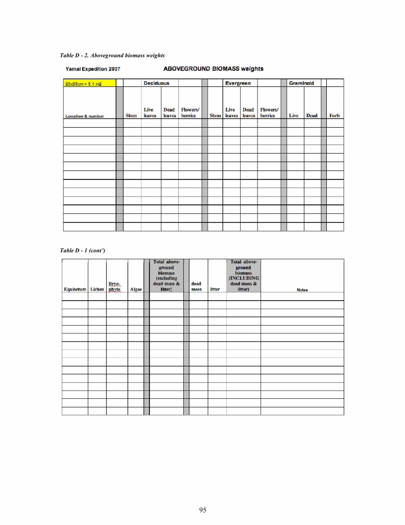
95
Table D - 2. Aboveground biomass weights
Table D - 1 (cont’)
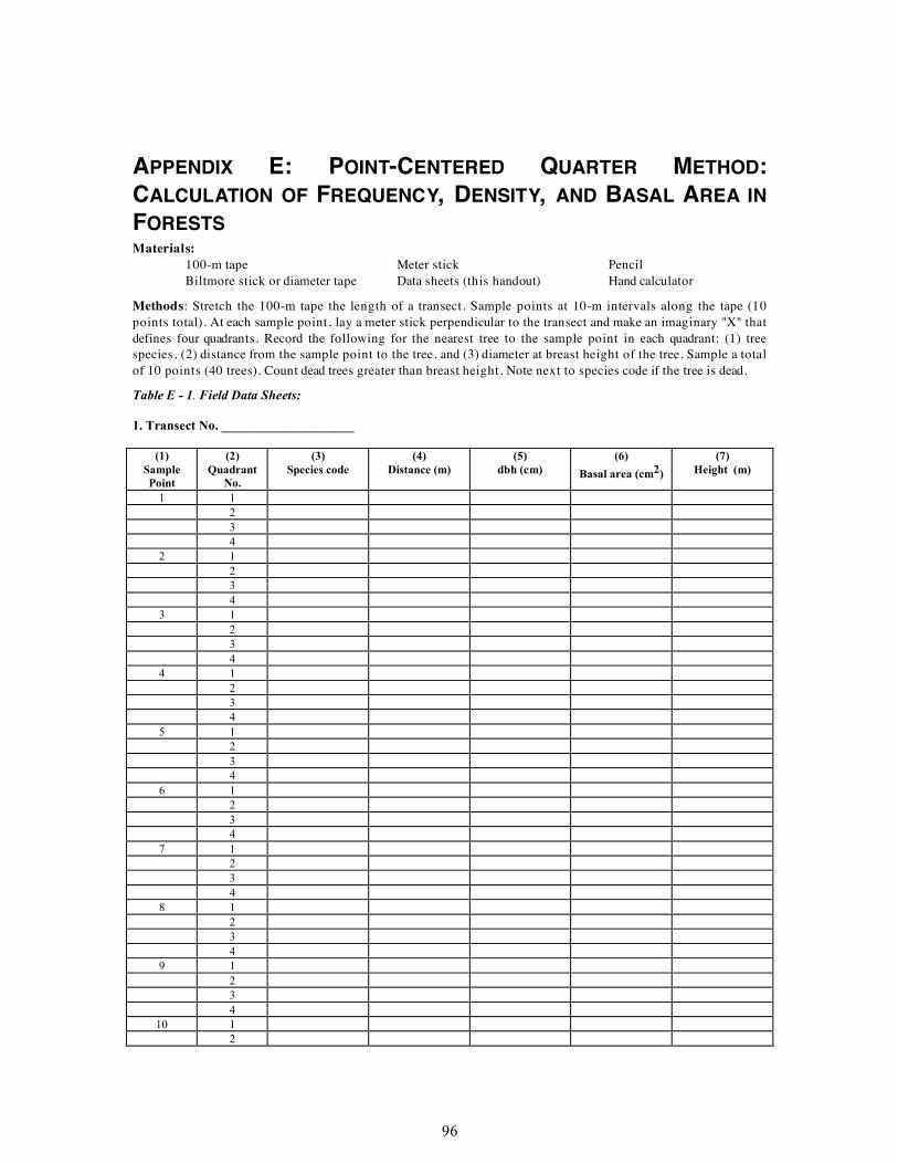
96
APPENDIX E: POINT-CENTERED QUARTER METHOD: CALCULATION OF FREQUENCY, DENSITY, AND BASAL AREA IN FORESTS Materials:
100-m tape Meter stick Pencil Biltmore stick or diameter tape Data sheets (this handout) Hand calculator
Methods: Stretch the 100-m tape the length of a transect. Sample points at 10-m intervals along the tape (10 points total). At each sample point, lay a meter stick perpendicular to the transect and make an imaginary "X" that defines four quadrants. Record the following for the nearest tree to the sample point in each quadrant: (1) tree species, (2) distance from the sample point to the tree, and (3) diameter at breast height of the tree. Sample a total of 10 points (40 trees). Count dead trees greater than breast height. Note next to species code if the tree is dead.
Table E - 1. Field Data Sheets: 1. Transect No. ____________________
(1) Sample Point
(2) Quadrant
No.
(3) Species code
(4) Distance (m)
(5) dbh (cm)
(6) Basal area (cm2)
(7) Height (m)
1 1 2 3 4 2 1 2 3 4 3 1 2 3 4 4 1 2 3 4 5 1 2 3 4 6 1 2 3 4 7 1 2 3 4 8 1 2 3 4 9 1 2 3 4
10 1 2
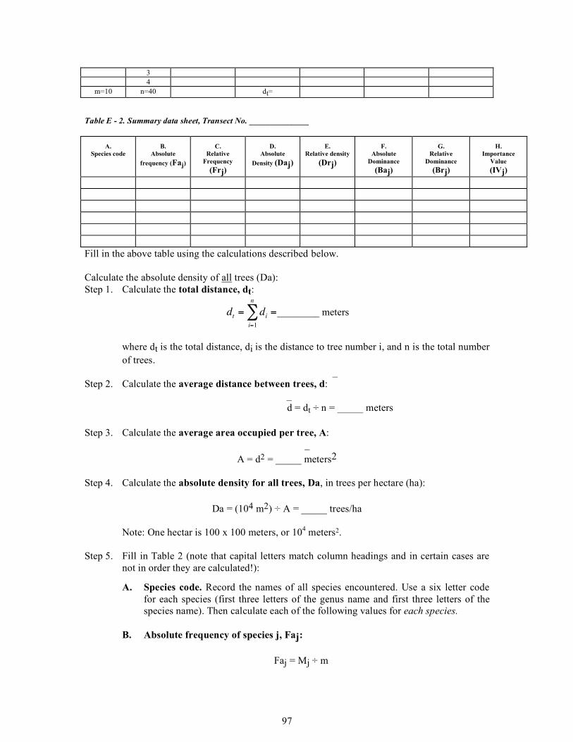
97
3 4
m=10 n=40 dt=
Table E - 2. Summary data sheet, Transect No. ______________
A.
Species code B.
Absolute frequency (Faj)
C. Relative
Frequency (Frj)
D. Absolute
Density (Daj)
E. Relative density
(Drj)
F. Absolute
Dominance (Baj)
G. Relative
Dominance (Brj)
H. Importance
Value (IVj)
Fill in the above table using the calculations described below. Calculate the absolute density of all trees (Da): Step 1. Calculate the total distance, dt:
!
dt
= di
i=1
n
" =_________ meters
where dt is the total distance, di is the distance to tree number i, and n is the total number
of trees. _ Step 2. Calculate the average distance between trees, d: _
d = dt ÷ n = _____ meters Step 3. Calculate the average area occupied per tree, A: _
A = d2 = _____ meters2 Step 4. Calculate the absolute density for all trees, Da, in trees per hectare (ha):
Da = (104 m2) ÷ A = _____ trees/ha Note: One hectar is 100 x 100 meters, or 104 meters2. Step 5. Fill in Table 2 (note that capital letters match column headings and in certain cases are
not in order they are calculated!):
A. Species code. Record the names of all species encountered. Use a six letter code for each species (first three letters of the genus name and first three letters of the species name). Then calculate each of the following values for each species.
B. Absolute frequency of species j, Faj:
Faj = Mj ÷ m
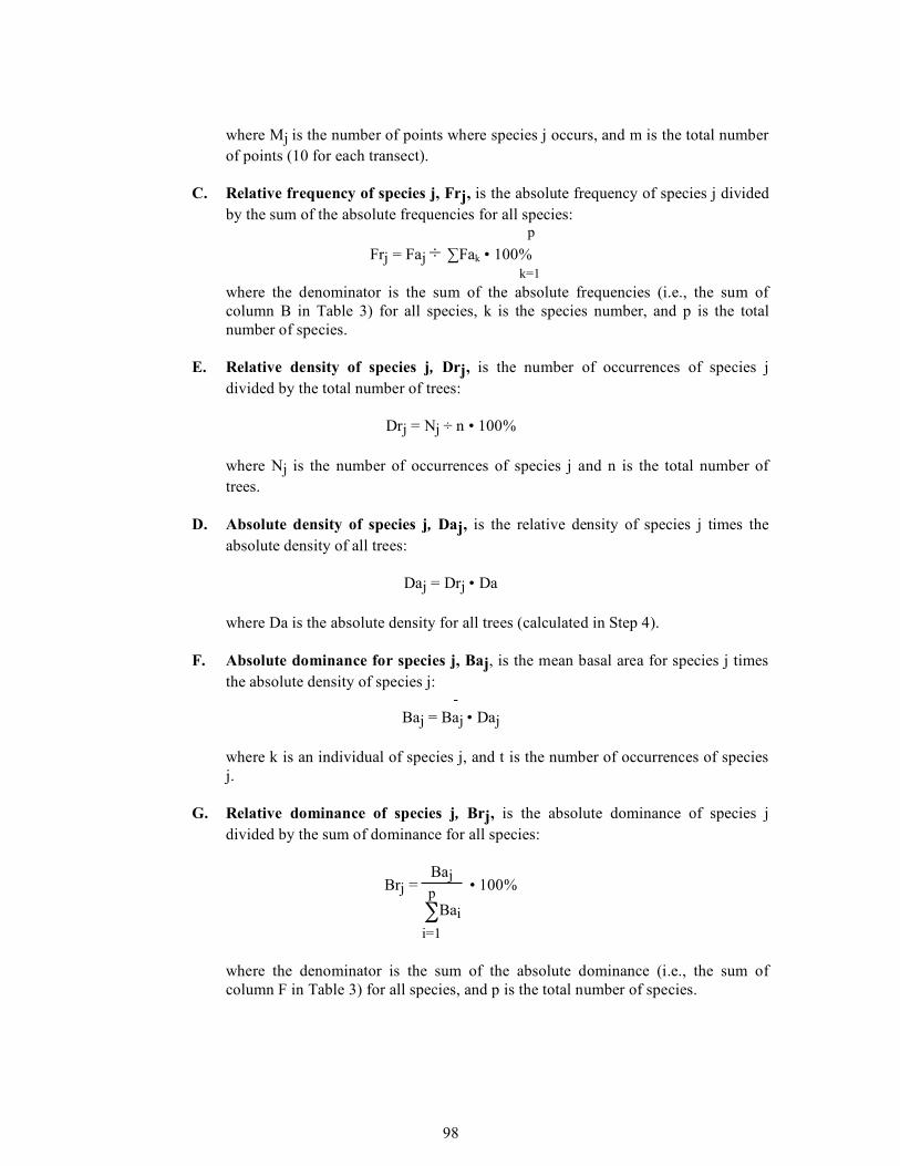
98
where Mj is the number of points where species j occurs, and m is the total number
of points (10 for each transect). C. Relative frequency of species j, Frj, is the absolute frequency of species j divided
by the sum of the absolute frequencies for all species: p
Frj = Faj ÷ ∑Fak • 100% k=1 where the denominator is the sum of the absolute frequencies (i.e., the sum of
column B in Table 3) for all species, k is the species number, and p is the total number of species.
E. Relative density of species j, Drj, is the number of occurrences of species j
divided by the total number of trees:
Drj = Nj ÷ n • 100%
where Nj is the number of occurrences of species j and n is the total number of trees.
D. Absolute density of species j, Daj, is the relative density of species j times the
absolute density of all trees:
Daj = Drj • Da where Da is the absolute density for all trees (calculated in Step 4). F. Absolute dominance for species j, Baj, is the mean basal area for species j times
the absolute density of species j: -
Baj = Baj • Daj
where k is an individual of species j, and t is the number of occurrences of species j.
G. Relative dominance of species j, Brj, is the absolute dominance of species j
divided by the sum of dominance for all species:
Brj = Baj
∑i=1
pBai
• 100%
where the denominator is the sum of the absolute dominance (i.e., the sum of
column F in Table 3) for all species, and p is the total number of species.

99
H. Importance value for species j, IVj, is the sum of the relative frequency, relative density, and relative dominance for the species:
IVj= Frj + Drj + Brj

100
APPE
NDIX
F: P
LOT
SOIL
AND
VEG
ETAT
ION
PHO
TOS
Key
:
ND
Nad
ym
LA L
abor
avay
a
V
D V
aski
ny D
achi
R
V R
elev
é

101
Fig
ure
F -
1. S
oils
– N
adym
1
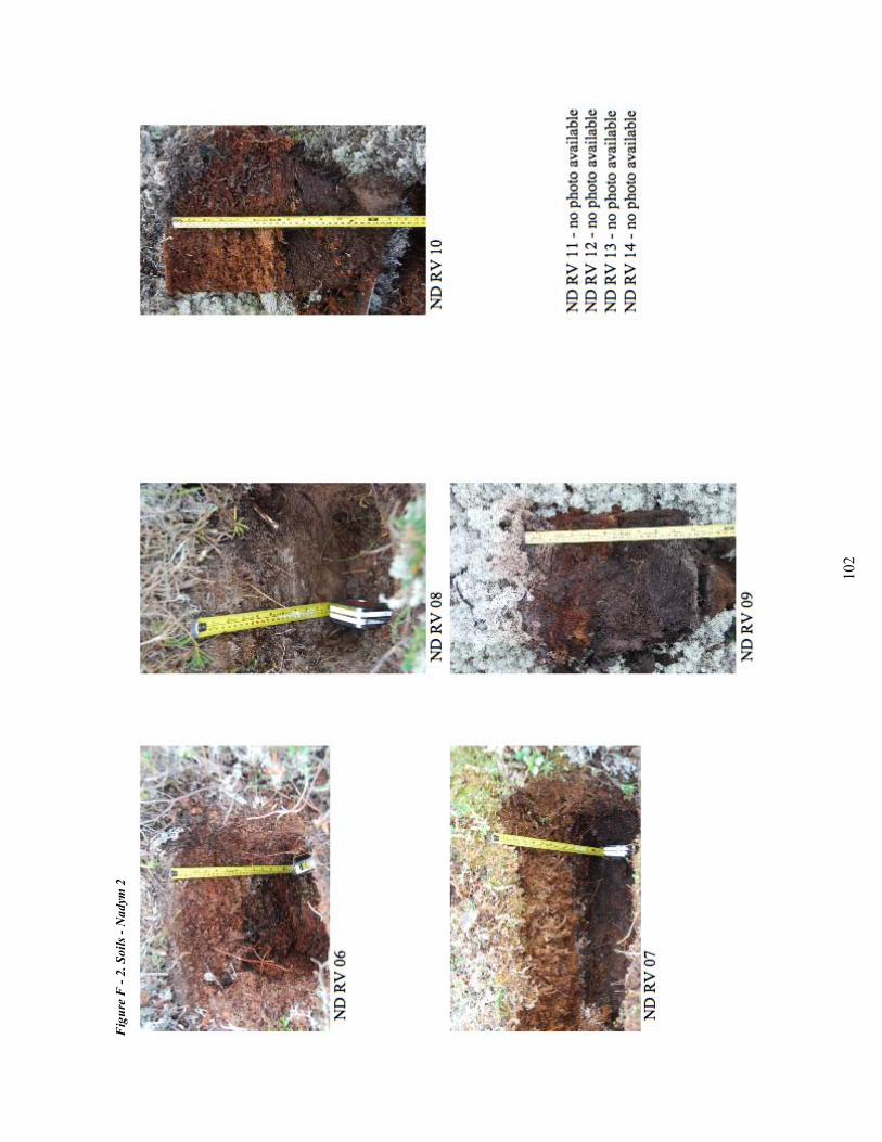
102
Fig
ure
F -
2. S
oils
- N
adym
2
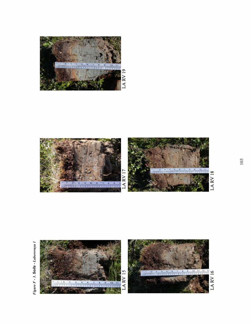
103
Fig
ure
F -
3. S
oils
- La
boro
vaya
1
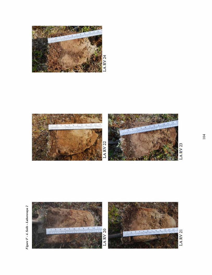
104
Fig
ure
F -
4. S
oils
- La
boro
vaya
2
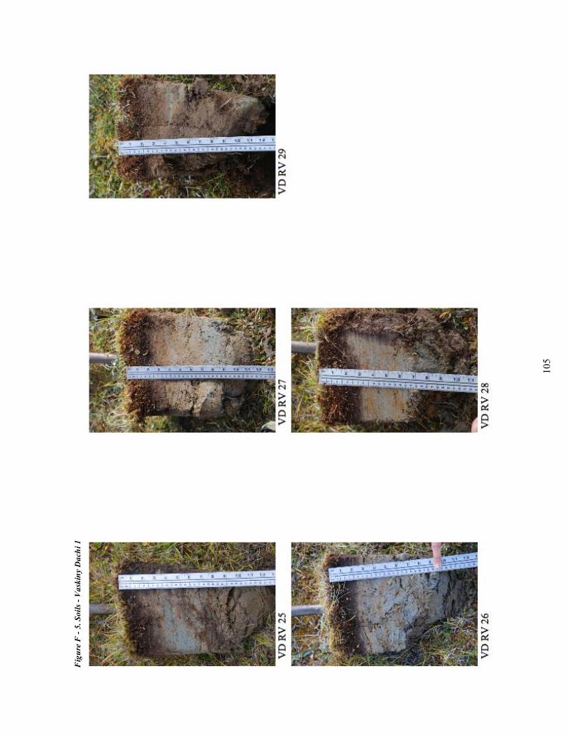
105
Fig
ure
F -
5. S
oils
- V
aski
ny D
achi
1
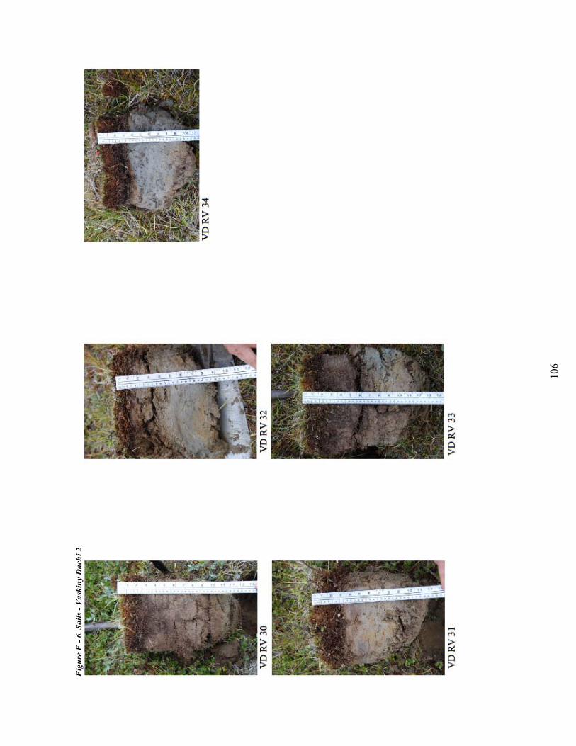
106
Fig
ure
F -
6. S
oils
- V
aski
ny D
achi
2
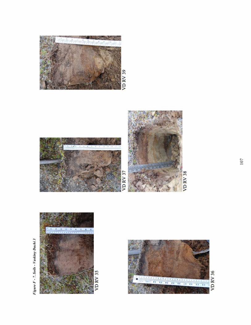
107
Fig
ure
F -
7. S
oils
- V
aski
ny D
achi
3
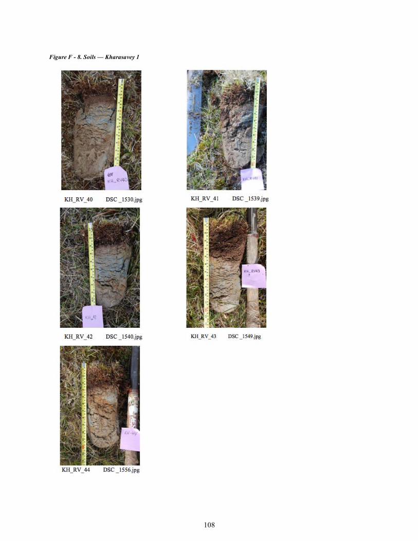
108
Figure F - 8. Soils — Kharasavey 1

109
Figure F - 9. Soils — Kharasavey-2a, -2b, and RV-49
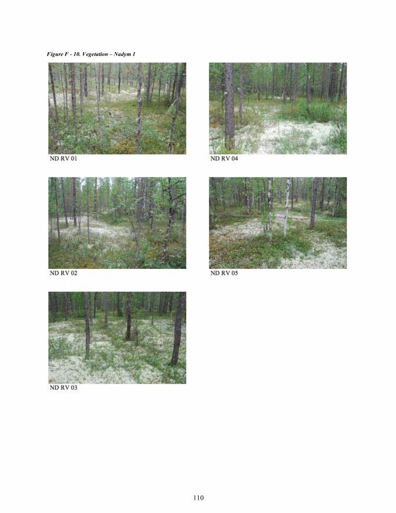
110
Figure F - 10. Vegetation – Nadym 1
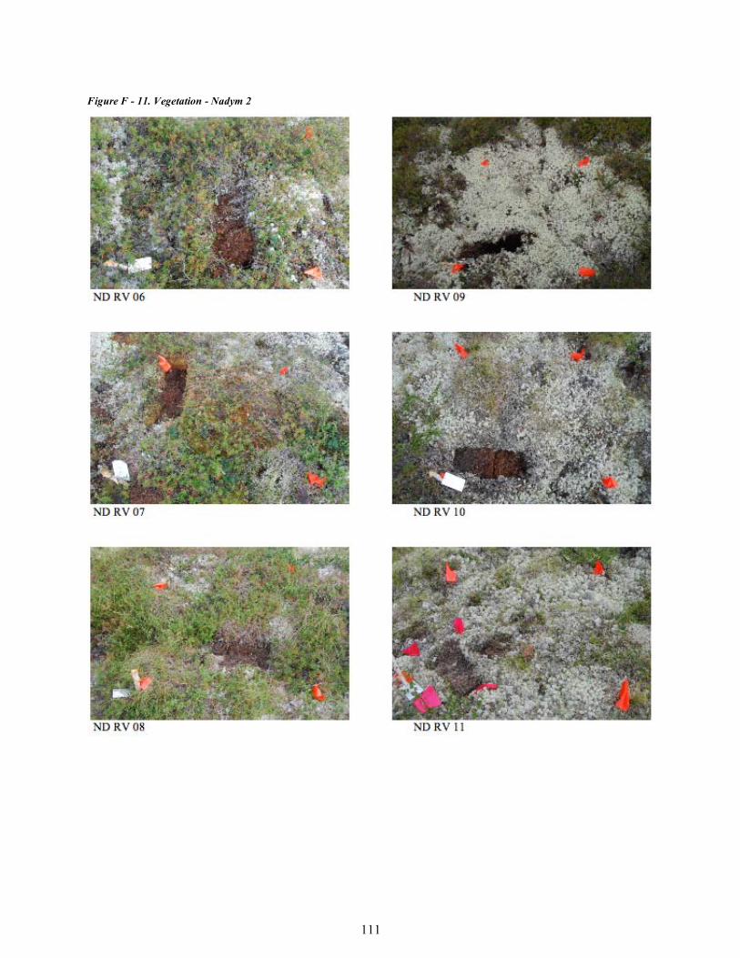
111
Figure F - 11. Vegetation - Nadym 2
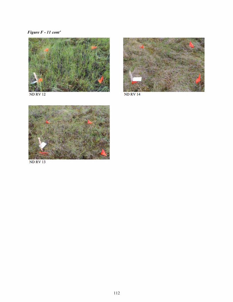
112
Figure F - 11 cont’
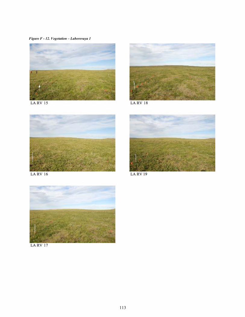
113
Figure F - 12. Vegetation – Laborovaya 1
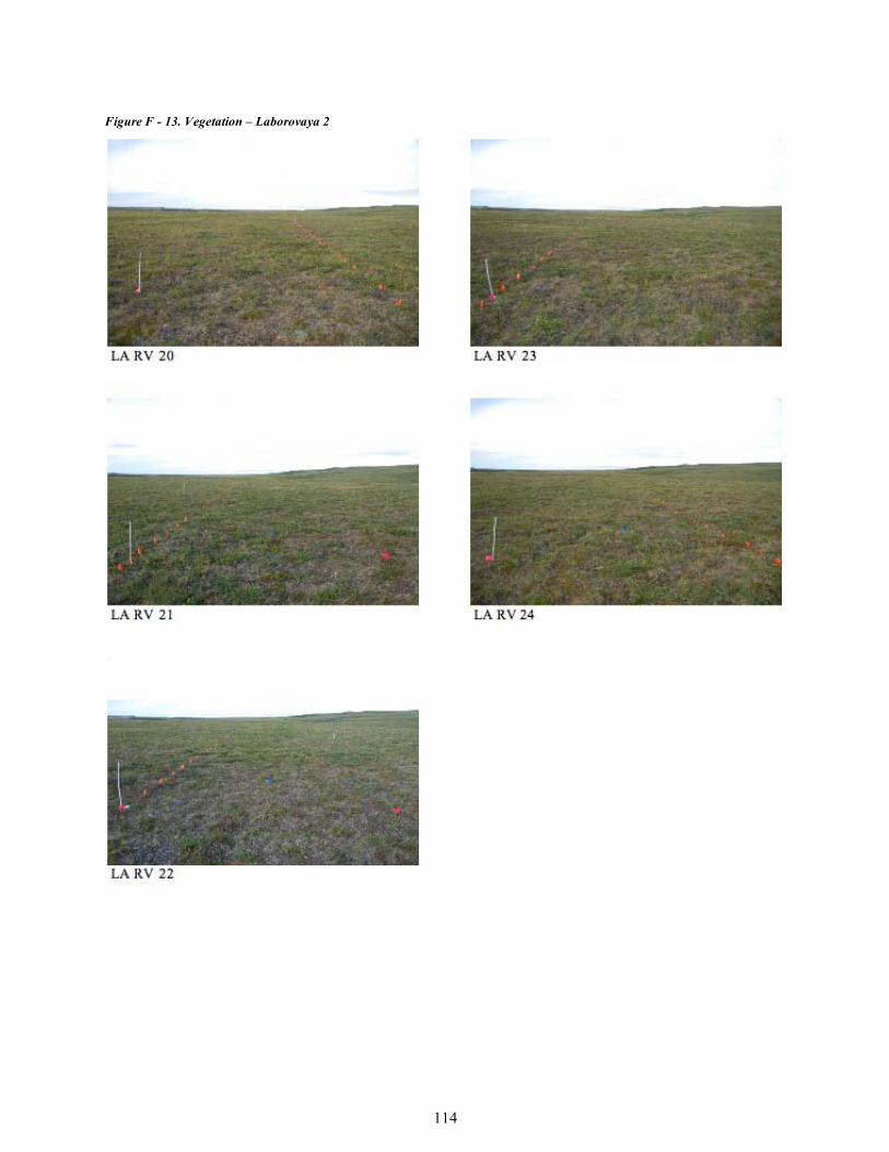
114
Figure F - 13. Vegetation – Laborovaya 2

115
Figure F - 14. Vegetation – Vaskiny Dachi 1
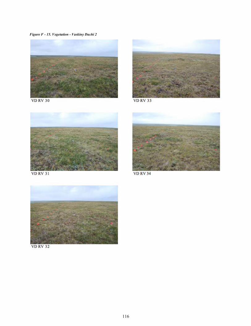
116
Figure F - 15. Vegetation - Vaskiny Dachi 2
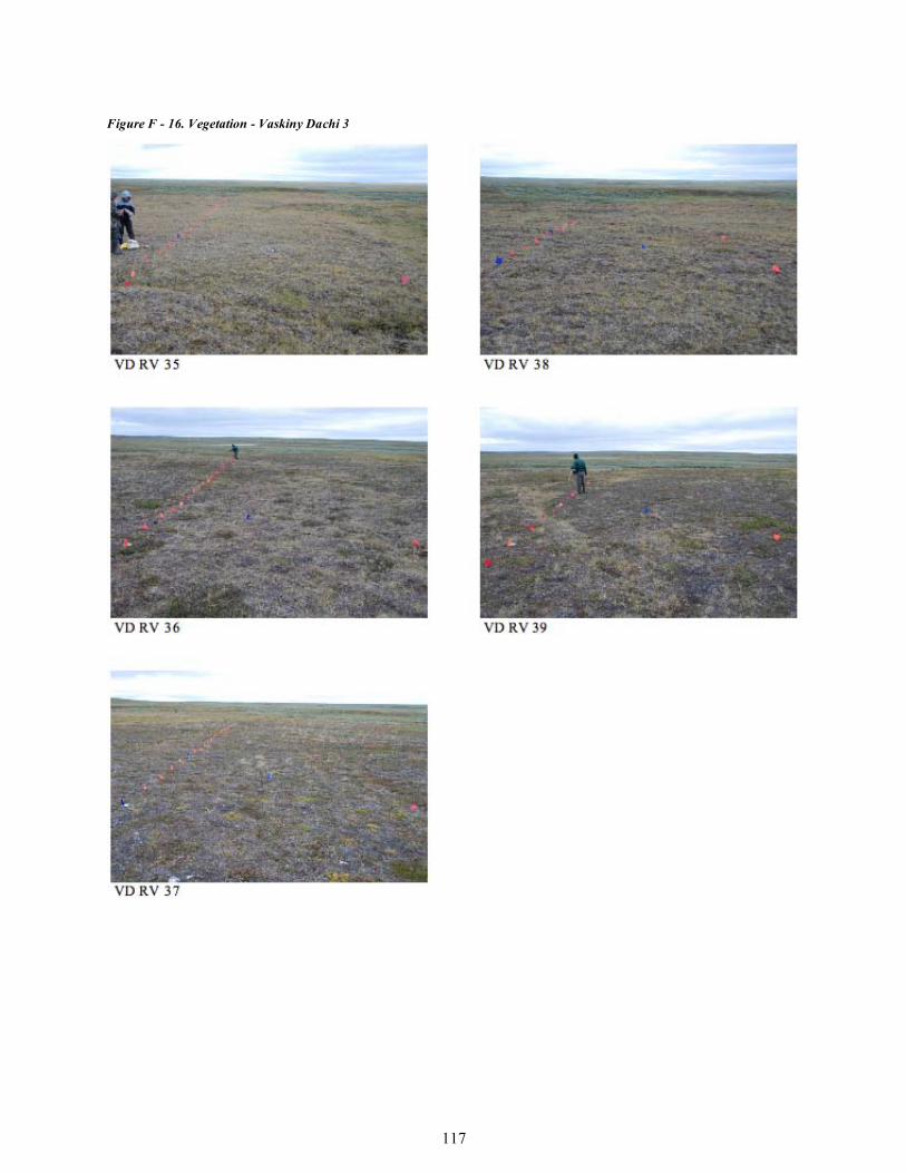
117
Figure F - 16. Vegetation - Vaskiny Dachi 3
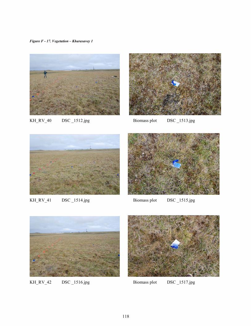
118
Figure F - 17. Vegetation – Kharasavey 1
KH_RV_40 DSC _1512.jpg Biomass plot DSC _1513.jpg
KH_RV_41 DSC _1514.jpg Biomass plot DSC _1515.jpg
KH_RV_42 DSC _1516.jpg Biomass plot DSC _1517.jpg
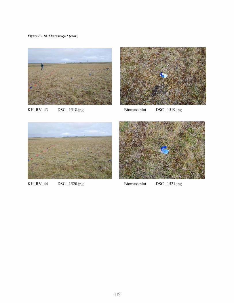
119
Figure F - 18. Kharasavey-1 (cont’)
KH_RV_43 DSC _1518.jpg Biomass plot DSC _1519.jpg
KH_RV_44 DSC _1520.jpg Biomass plot DSC _1521.jpg
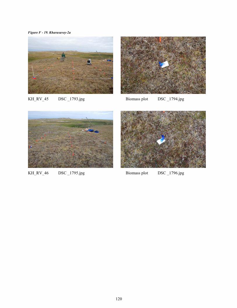
120
Figure F - 19. Kharasavey-2a
KH_RV_45 DSC _1793.jpg Biomass plot DSC _1794.jpg
KH_RV_46 DSC _1795.jpg Biomass plot DSC _1796.jpg
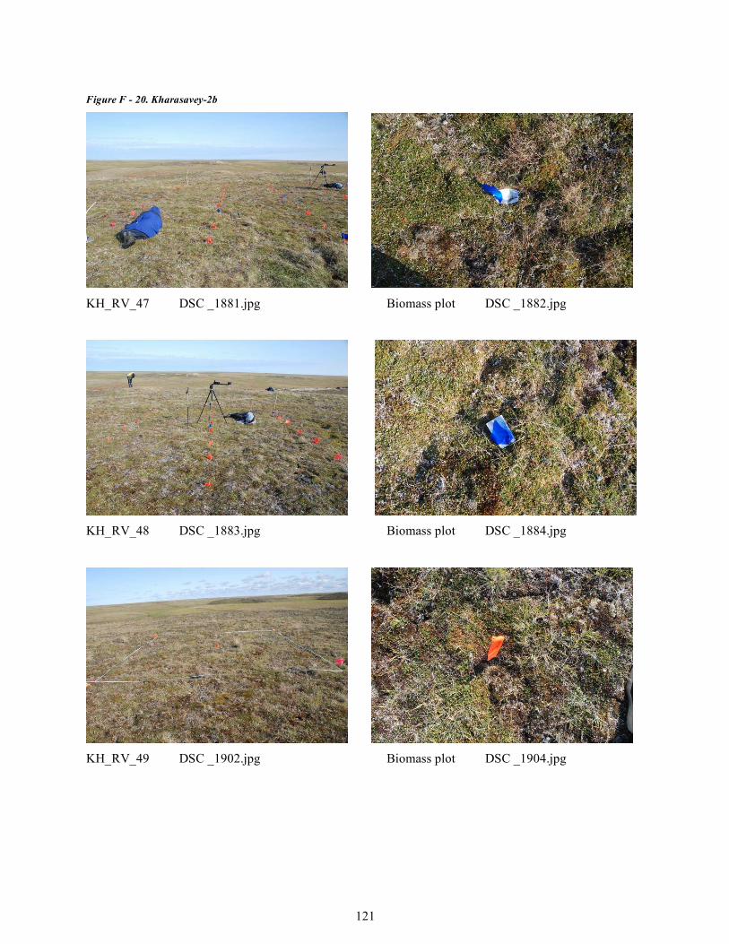
121
Figure F - 20. Kharasavey-2b
KH_RV_47 DSC _1881.jpg Biomass plot DSC _1882.jpg
KH_RV_48 DSC _1883.jpg Biomass plot DSC _1884.jpg
KH_RV_49 DSC _1902.jpg Biomass plot DSC _1904.jpg