Data Mining Taylor Statistics 202: Data...
56
Statistics 202: Data Mining c Jonathan Taylor Statistics 202: Data Mining Classification & Decision Trees Based in part on slides from textbook, slides of Susan Holmes c Jonathan Taylor October 19, 2012 1/1
Transcript of Data Mining Taylor Statistics 202: Data...

Statistics 202:Data Mining
c©JonathanTaylor
Statistics 202: Data MiningClassification & Decision Trees
Based in part on slides from textbook, slides of Susan Holmes
c©Jonathan Taylor
October 19, 2012
1 / 1

Statistics 202:Data Mining
c©JonathanTaylor
Classification
Problem description
We are given a data matrix XXX with either continuous ordiscrete variables such that each row Xi ∈ F and a set oflabels YYY ∈ L.
For a k-class problem, #L = k and we can think ofL = {1, . . . , k}.Our goal is to find a classifier
f : F → L
that allows us to predict the label of a new observationgiven a new set of features.
2 / 1

Statistics 202:Data Mining
c©JonathanTaylor
Classification
A supervised problem
Classification is a supervised problem.
Usually, we use a subset of the data, the training set tolearn or estimate the classifier yielding f = ftraining .
The performance of f is measured by applying it to eachcase in the test set and computing∑
j∈testL(ftraining (XXX j),YYY j)
3 / 1

Statistics 202:Data Mining
c©JonathanTaylor
Classification
4 / 1

Statistics 202:Data Mining
c©JonathanTaylor
Classification
Examples of classification tasks
Predicting whether a tumor is benign or malignant.
Classifying credit card transactions as fraudulent orlegitimate.
Predicting the type of a given tumor among several types.
Cateogrizing a document or news story as one of {finance,weather, sports, etc.}
5 / 1

Statistics 202:Data Mining
c©JonathanTaylor
Classification
Common techniques
Decision Tree based Methods
Rule-based Methods
Discriminant Analysis
Memory based reasoning
Neural Networks
Naıve Bayes
Support Vector Machines
6 / 1

Statistics 202:Data Mining
c©JonathanTaylor
Classification trees
7 / 1

Statistics 202:Data Mining
c©JonathanTaylor
Classification trees
8 / 1
Statistics 202:Data Mining
c©JonathanTaylor
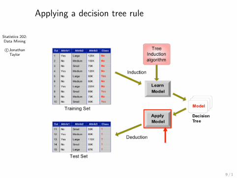
Applying a decision tree rule
9 / 1

Statistics 202:Data Mining
c©JonathanTaylor
Applying a decision tree rule
10 / 1

Statistics 202:Data Mining
c©JonathanTaylor
Applying a decision tree rule
11 / 1

Statistics 202:Data Mining
c©JonathanTaylor
Applying a decision tree rule
12 / 1

Statistics 202:Data Mining
c©JonathanTaylor
Applying a decision tree rule
13 / 1

Statistics 202:Data Mining
c©JonathanTaylor
Applying a decision tree rule
14 / 1

Statistics 202:Data Mining
c©JonathanTaylor
Applying a decision tree rule
15 / 1

Statistics 202:Data Mining
c©JonathanTaylor
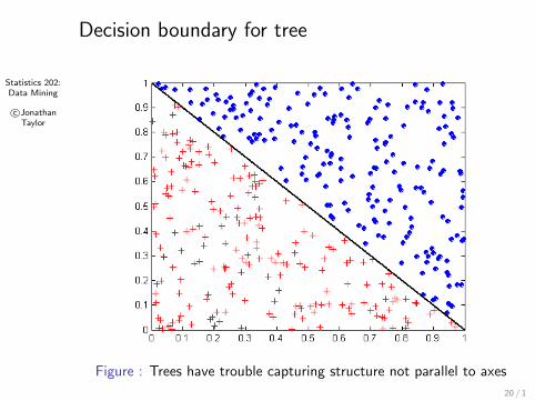
Decision boundary for tree
16 / 1

Statistics 202:Data Mining
c©JonathanTaylor
Decision tree for iris data using all features
17 / 1

Statistics 202:Data Mining
c©JonathanTaylor
Decision tree for iris data using petal.length,
petal.width
18 / 1

Statistics 202:Data Mining
c©JonathanTaylor
Regions in petal.length, petal.width plane
0 1 2 3 4 5 6 7 8Petal length
0.5
0.0
0.5
1.0
1.5
2.0
2.5
3.0
Peta
l w
idth
19 / 1
Statistics 202:Data Mining
c©JonathanTaylor
Decision boundary for tree
Figure : Trees have trouble capturing structure not parallel to axes
20 / 1

Statistics 202:Data Mining
c©JonathanTaylor
Learning the tree
21 / 1

Statistics 202:Data Mining
c©JonathanTaylor
Learning the tree
Hunt’s algorithm (generic structure)
Let Dt be the set of training records that reach a node t
If Dt contains records that belong the same class yt , thent is a leaf node labeled as yt .
If Dt = ∅, then t is a leaf node labeled by the defaultclass, yd .
If Dt contains records that belong to more than one class,use an attribute test to split the data into smaller subsets.Recursively apply the procedure to each subset.
This splitting procedure is what can vary for different treelearning algorithms . . .
22 / 1

Statistics 202:Data Mining
c©JonathanTaylor
Learning the tree
23 / 1

Statistics 202:Data Mining
c©JonathanTaylor
Learning the tree
Issues
Greedy strategy: Split the records based on an attribute testthat optimizes certain criterion.
What is the best split: What criterion do we use? Previousexample chose first to split on Refund . . .
How to split the records: Binary or multi-way? Previousexample split Taxable Income at ≥ 80K . . .
When do we stop? Should we continue until each node if possible? Previousexample stopped with all nodes being completely homogeneous. . .
24 / 1

Statistics 202:Data Mining
c©JonathanTaylor
Different splits: ordinal / nominal
Figure : Binary or multi-way?
25 / 1

Statistics 202:Data Mining
c©JonathanTaylor
Different splits: continuous
Figure : Binary or multi-way?
26 / 1

Statistics 202:Data Mining
c©JonathanTaylor
Choosing a variable to split on
Figure : Which should we start the splitting on?
27 / 1
Statistics 202:Data Mining
c©JonathanTaylor
Learning the tree
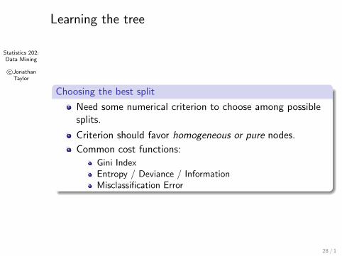
Choosing the best split
Need some numerical criterion to choose among possiblesplits.
Criterion should favor homogeneous or pure nodes.
Common cost functions:
Gini IndexEntropy / Deviance / InformationMisclassification Error
28 / 1

Statistics 202:Data Mining
c©JonathanTaylor
Choosing a variable to split on
29 / 1

Statistics 202:Data Mining
c©JonathanTaylor
Learning the tree
GINI Index
Suppose we have k classes and node t has frequenciespt = (p1,t , . . . , pk,t).
Criterion
GINI (t) =∑
(j ,j ′)∈{1,...,k}:j 6=j ′
pj ,tpj ′,t = 1−l∑
j=1
p2j ,t .
Maximized when pj ,t = 1/k with value 1− 1/k
Minimized when all records belong to a single class.
Minimizing GINI will favour pure nodes . . .
30 / 1

Statistics 202:Data Mining
c©JonathanTaylor
Learning the tree
Gain in GINI Index for a potential split
Suppose t is to be split into j new child nodes (tl)1≤l≤j .
Each child node has a count nl and a vector of frequencies(p1,tl , . . . , pk,tl ). Hence they have their own GINI index,GINI (tl).
The gain in GINI Index for this split is
Gain(GINI , t → (tl)1≤l≤j) = GINI (t)−∑j
l=1 nlGINI (tl)∑jl=1 nl
.
Greedy algorithm chooses the biggest gain in GINI indexamong a list of possible splits.
31 / 1
Statistics 202:Data Mining
c©JonathanTaylor
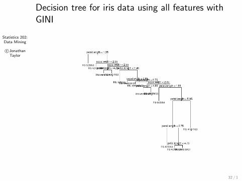
Decision tree for iris data using all features withGINI
32 / 1

Statistics 202:Data Mining
c©JonathanTaylor
Learning the tree
Entropy / Deviance / Information
Suppose we have k classes and node t has frequenciespt = (p1,t , . . . , pk,t).
Criterion
H(t) = −k∑
j=1
pj ,t log pj ,t
Maximized when pi ,t = 1/k with value log k
Minimized when one class has no records in it.
Minimizing entropy will favour pure nodes . . .
33 / 1

Statistics 202:Data Mining
c©JonathanTaylor
Decision tree for iris data using all features withEntropy
34 / 1

Statistics 202:Data Mining
c©JonathanTaylor
Learning the tree
Gain in entropy for a potential split
Suppose t is to be split into j new child nodes (tl)1≤l≤j .
Each child node has a count nl and a vector of frequencies(p1,tl , . . . , pk,tl ). Hence they have their own entropy H(tl).
The gain in entropy for this split is
Gain(H, t → (tl)1≤l≤j) = H(t)−∑j
l=1 nlH(tl)∑jl=1 nl
.
Greedy algorithm chooses the biggest gain in H among alist of possible splits.
35 / 1

Statistics 202:Data Mining
c©JonathanTaylor
Learning the tree
Misclassification Error
Suppose we have k classes and node t has frequenciespt = (p1,t , . . . , pk,t).
The mode isk(t) = argmax
kpk,t .
Criterion
Misclassification Error(t) = 1− pk(t),t
Not smooth in pt as GINI ,H, can be more difficult tooptimize numerically.
36 / 1

Statistics 202:Data Mining
c©JonathanTaylor
Different criteria: GINI , H , MC
37 / 1

Statistics 202:Data Mining
c©JonathanTaylor
Learning the tree
Misclassification Error
Example: suppose parent has 10 cases: {7D, 3R}A candidate split produces two nodes: {3D, 0R},{4D, 3R}.The gain in MC is 0, but gain in GINI is 0.42− 0.342 > 0.
Similarly, entropy will also show an improvement . . .
38 / 1
Statistics 202:Data Mining
c©JonathanTaylor
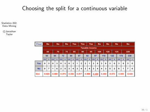
Choosing the split for a continuous variable
39 / 1

Statistics 202:Data Mining
c©JonathanTaylor
Learning the tree
Stopping training
As trees get deeper, or if splits are multi-way the numberof data points per leaf node drops very quickly.
Trees that are too deep tend to overfit the data.
A common strategy is to “prune” the tree by removingsome internal nodes.
40 / 1

Statistics 202:Data Mining
c©JonathanTaylor
Learning the tree
Figure : Underfitting corresponds to the left-hand side, overfit to theright
41 / 1
Statistics 202:Data Mining
c©JonathanTaylor
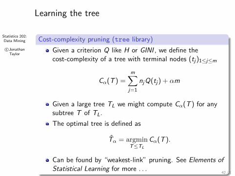
Learning the tree
Cost-complexity pruning (tree library)
Given a criterion Q like H or GINI , we define thecost-complexity of a tree with terminal nodes (tj)1≤j≤m
Cα(T ) =m∑j=1
njQ(tj) + αm
Given a large tree TL we might compute Cα(T ) for anysubtree T of TL.
The optimal tree is defined as
Tα = argminT≤TL
Cα(T ).
Can be found by “weakest-link” pruning. See Elements ofStatistical Learning for more . . .
42 / 1

Statistics 202:Data Mining
c©JonathanTaylor
Learning the tree
Pre-pruning (rpart library)
These methods stop the algorithm before it becomes afully-grown tree.
Examples
Stop if all instances belong to the same class (kind ofobvious).Stop if number of instances is less than some user-specifiedthreshold. Both tree, rpart have rules like this.Stop if class distribution of instances are independent ofthe available features (e.g., using χ2 test)Stop if expanding the current node does not improveimpurity measures (e.g., Gini or information gain). Thisrelates to cp in rpart.
43 / 1

Statistics 202:Data Mining
c©JonathanTaylor
Training and test error as a function of cp
44 / 1
Statistics 202:Data Mining
c©JonathanTaylor
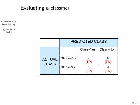
Evaluating a classifier
© Tan,Steinbach, Kumar Introduction to Data Mining 4/18/2004
Metrics for Performance Evaluation…
l Most widely-used metric:
PREDICTED CLASSPREDICTED CLASSPREDICTED CLASS
ACTUALCLASS
Class=Yes Class=No
ACTUALCLASS
Class=Yes a(TP)
b(FN)
ACTUALCLASS
Class=No c(FP)
d(TN)
45 / 1

Statistics 202:Data Mining
c©JonathanTaylor
Evaluating a classifier
Measures of performance
Simplest is accuracy
Accuracy =TP + TN
TP + TN + FP + FN
= SMC(Actual,Predicted)
= 1−Misclassification Rate
46 / 1
Statistics 202:Data Mining
c©JonathanTaylor
Evaluating a classifier
Accuracy isn’t everything
Consider an unbalanced 2-class problem with # 1’s=10, #0’s=9990.
Simply labelling everything 0 yields 99.9% accuracy.
But, this classifier misses all class 1.
47 / 1

Statistics 202:Data Mining
c©JonathanTaylor
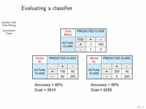
Evaluating a classifier
© Tan,Steinbach, Kumar Introduction to Data Mining 4/18/2004
Cost Matrix
PREDICTED CLASS PREDICTED CLASS PREDICTED CLASS
ACTUALCLASS
C(i|j) Class=Yes Class=No
ACTUALCLASS
Class=Yes C(Yes|Yes) C(No|Yes)ACTUALCLASS
Class=No C(Yes|No) C(No|No)
C(i|j): Cost of misclassifying class j example as class i
48 / 1

Statistics 202:Data Mining
c©JonathanTaylor
Learning the tree
Measures of performance
Classification rule changes to
Label(p,C ) = argmini∑j
C (i |j)pj
Accuracy is the same as cost if C (Y |Y ) = C (N|N) = c1,C (Y |N) = C (N|Y ) = c2.
49 / 1
Statistics 202:Data Mining
c©JonathanTaylor
Evaluating a classifier
© Tan,Steinbach, Kumar Introduction to Data Mining 4/18/2004
Computing Cost of Classification
Cost Matrix
PREDICTED CLASSPREDICTED CLASSPREDICTED CLASS
ACTUALCLASS
C(i|j) + -ACTUALCLASS + -1 100ACTUALCLASS
- 1 0
Model M1
PREDICTED CLASSPREDICTED CLASSPREDICTED CLASS
ACTUALCLASS
+ -ACTUALCLASS + 150 40ACTUALCLASS
- 60 250
Model M2
PREDICTED CLASSPREDICTED CLASSPREDICTED CLASS
ACTUALCLASS
+ -ACTUALCLASS + 250 45ACTUALCLASS
- 5 200
Accuracy = 80%Cost = 3910
Accuracy = 90%Cost = 4255
50 / 1
Statistics 202:Data Mining
c©JonathanTaylor
Evaluating a classifier
Measures of performance
Other common ones
Precision =TP
TP + FP
Specificity =TN
TN + FP= TNR
Sensitivity = Recall =TP
TP + FN= TPR
F =2 · Recall · Precision
Recall + Precision
=2 · TP
2 · TP + FN + FP
51 / 1
Statistics 202:Data Mining
c©JonathanTaylor
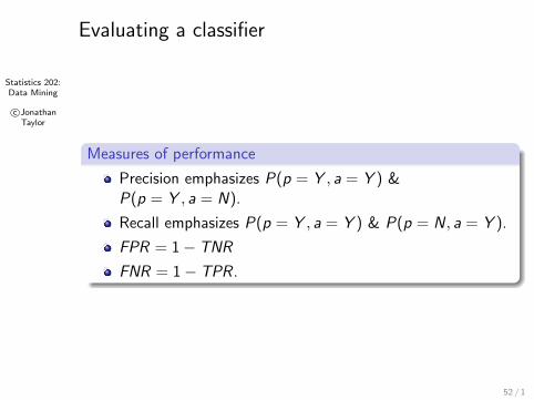
Evaluating a classifier
Measures of performance
Precision emphasizes P(p = Y , a = Y ) &P(p = Y , a = N).
Recall emphasizes P(p = Y , a = Y ) & P(p = N, a = Y ).
FPR = 1− TNR
FNR = 1− TPR.
52 / 1

Statistics 202:Data Mining
c©JonathanTaylor
Evaluating a classifier
Measure of performance
We have done some simple training / test splits to seehow well our classifier is doing.
More accurately, this procedure measures how well ouralgorithm for learning the classifier is doing.
How well this works may depend on
Model: Are we using the right type of classifiermodel?
Cost: Is our algorithm sensitive to the cost ofmisclassification?
Data size: Do we have enough data to learn a model?
53 / 1

Statistics 202:Data Mining
c©JonathanTaylor
Evaluating a classifier
© Tan,Steinbach, Kumar Introduction to Data Mining 4/18/2004
Learning Curve
l Learning curve shows how accuracy changes with varying sample size
l Requires a sampling schedule for creating learning curve:
l Arithmetic sampling(Langley, et al)
l Geometric sampling(Provost et al)
Effect of small sample size:- Bias in the estimate- Variance of estimate
Figure : As data increases, our estimate of accuracy improves, asdoes the variability of our estimate . . .
54 / 1

Statistics 202:Data Mining
c©JonathanTaylor
Evaluating a classifier
Estimating performance
Holdout: Split into test and training (e.g. 1/3 test, 2/3training).
Random subsampling: Repeated replicates of holdout,averaging results.
Cross validation: Partition data into K disjoint subsets. Foreach subset Si , train on all but Si , then test onSi .
Stratified sampling: May be helpful to sample so Y/N class isroughly equal in training data.
0.632 Bootstrap: Combine training error and bootstrap error. . .
55 / 1

Statistics 202:Data Mining
c©JonathanTaylor
56 / 1