Data Mining on NIJ dataData Mining on NIJ data

Sangjik Lee

Unstructured Data MiningUnstructured Data Mining

Text

Keyword Extraction

Structured Data Base

Data Mining

Image

Feature Extraction

Structured Data Base

Data Mining

Handwritten CEDAR Letter

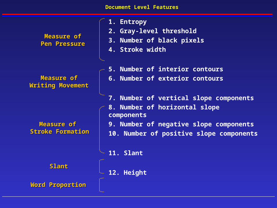
Document Level FeaturesDocument Level Features

1. Entropy

2. Gray-level threshold

3. Number of black pixels

4. Stroke width

5. Number of interior contours

6. Number of exterior contours

7. Number of vertical slope components

8. Number of horizontal slope components

9. Number of negative slope components

10. Number of positive slope components

11. Slant

12. Height

Measure ofMeasure ofPen PressurePen Pressure

Measure ofMeasure ofWriting MovementWriting Movement

Measure of Measure of Stroke FormationStroke Formation

SlantSlant

Word ProportionWord Proportion

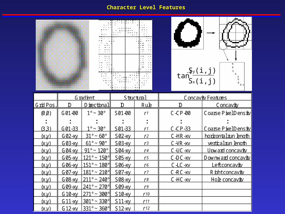
Character Level FeaturesCharacter Level Features

Sy(i,j)tan

Sx(i,j)-1

Grid Pos. ID Directional ID Rule ID Concavity

(0,0) G01-00 1° ~ 30° S01-00 r 1 C-CP-00 Coarse Pixel Density

: : : : : : :(3,3) G01-33 1° ~ 30° S01-33 r 1 C-CP-33 Coarse Pixel Density(x,y) G02-xy 31° ~ 60° S02-xy r 2 C-HR-xy horizontal run length(x,y) G03-xy 61° ~ 90° S03-xy r 3 C-VR-xy vertical run length(x,y) G04-xy 91° ~ 120° S04-xy r 4 C-UC-xy Upward concavity(x,y) G05-xy 121° ~ 150° S05-xy r 5 C-DC-xy Downward concavity(x,y) G06-xy 151° ~ 180° S06-xy r 6 C-LC-xy Left concavity(x,y) G07-xy 181° ~ 210° S07-xy r 7 C-RC-xy Right concavity(x,y) G08-xy 211° ~ 240° S08-xy r 8 C-HC-xy Hole concavity(x,y) G09-xy 241° ~ 270° S09-xy r 9(x,y) G10-xy 271° ~ 300° S10-xy r 10(x,y) G11-xy 301° ~ 330° S11-xy r 11(x,y) G12-xy 331° ~ 360° S12-xy r 12

Gradient Structural Concavity Features

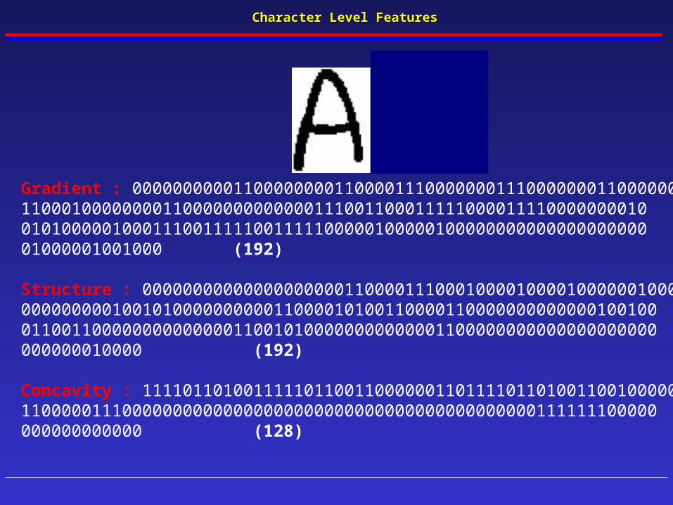
Gradient : 000000000011000000001100001110000000111000000011000000110001000000001100000000000001110011000111110000111100000000100101000001000111001111100111110000010000010000000000000000000001000001001000 (192)

Structure : 000000000000000000001100001110001000010000100000010000000000000100101000000000011000010100110000110000000000000100100011001100000000000000110010100000000000001100000000000000000000000000010000 (192)

Concavity : 11110110100111110110011000000110111101101001100100000110000011100000000000000000000000000000000000000000111111100000000000000000 (128)

Character Level FeaturesCharacter Level Features

Writer data Feature data (normalized)

Gen Age Han Edu Ethn Sch

M F <14 <24 <44 <64 <84 >85 L R H C H W B A O U F

0 1 0 0 1 0 0 0 0 1 0 1 0 0 0 1 0 0 1 .95 .49 .70 .71 .50 .10 .300 1 0 0 1 0 0 0 0 1 0 1 0 0 0 1 0 0 1 .94 .49 .75 .70 .50 .11 .300 1 0 0 1 0 0 0 0 1 0 1 0 0 0 1 0 0 1 .94 .49 .67 .74 .50 .10 .30

1 0 0 0 1 0 0 0 0 1 0 1 0 0 0 1 0 1 0 .93 .72 .33 .47 .50 .21 .281 0 0 0 1 0 0 0 0 1 0 1 0 0 0 1 0 1 0 .93 .74 .33 .48 .50 .22 .261 0 0 0 1 0 0 0 0 1 0 1 0 0 0 1 0 1 0 .93 .79 .36 .54 .50 .18 .27

1 0 0 0 1 0 0 0 0 1 0 1 0 0 0 1 0 0 1 .92 .30 .61 .66 .60 .11 .351 0 0 0 1 0 0 0 0 1 0 1 0 0 0 1 0 0 1 .94 .42 .72 .66 .60 .11 .321 0 0 0 1 0 0 0 0 1 0 1 0 0 0 1 0 0 1 .94 .40 .75 .67 .60 .12 .34

1 0 0 0 0 1 0 0 0 1 0 1 0 0 0 1 0 0 1 .96 .30 .60 .59 .50 .10 .211 0 0 0 0 1 0 0 0 1 0 1 0 0 0 1 0 0 1 .95 .32 .60 .59 .50 .09 .221 0 0 0 0 1 0 0 0 1 0 1 0 0 0 1 0 0 1 .95 .30 .66 .60 .50 .10 .21

dark blob hole slant width skew ht

int int int real int real int

Writer and Feature DataWriter and Feature Data

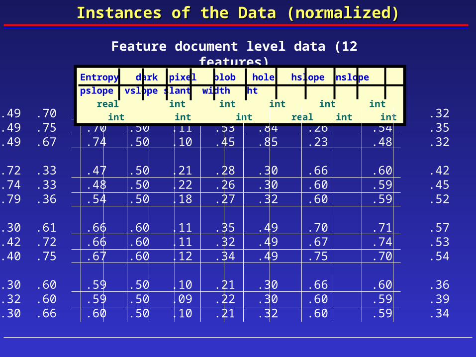
Instances of the Data (normalized)Instances of the Data (normalized)

Feature document level data (12 features)

.95 .49 .70 .71 .50 .10 .51 .92 .13 .47 .32 .21

.94 .49 .75 .70 .50 .11 .53 .84 .26 .54 .35 .18

.94 .49 .67 .74 .50 .10 .45 .85 .23 .48 .32 .22

.93 .72 .33 .47 .50 .21 .28 .30 .66 .60 .42 .10

.93 .74 .33 .48 .50 .22 .26 .30 .60 .59 .45 .10

.93 .79 .36 .54 .50 .18 .27 .32 .60 .59 .52 .09

.92 .30 .61 .66 .60 .11 .35 .49 .70 .71 .57 .10

.94 .42 .72 .66 .60 .11 .32 .49 .67 .74 .53 .10

.94 .40 .75 .67 .60 .12 .34 .49 .75 .70 .54 .11

.96 .30 .60 .59 .50 .10 .21 .30 .66 .60 .36 .10

.95 .32 .60 .59 .50 .09 .22 .30 .60 .59 .39 .10

.95 .30 .66 .60 .50 .10 .21 .32 .60 .59 .34 .09

Entropy dark pixel blob hole hslope nslope pslope vslope slant width ht

real int int int int int int int int real int int

White maleWhite female Black female Black male

Data Mining on sub-groupData Mining on sub-group

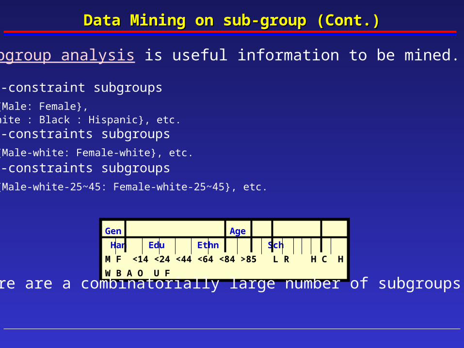
Data Mining on sub-group (Cont.)Data Mining on sub-group (Cont.)

Subgroup analysis is useful information to be mined.

• 1-constraint subgroups

{Male: Female}, {White : Black : Hispanic}, etc.• 2-constraints subgroups

{Male-white: Female-white}, etc. • 3-constraints subgroups

{Male-white-25~45: Female-white-25~45}, etc.

Gen Age Han Edu Ethn Sch

M F <14 <24 <44 <64 <84 >85 L R H C H W B A O U F

There are a combinatorially large number of subgroups.

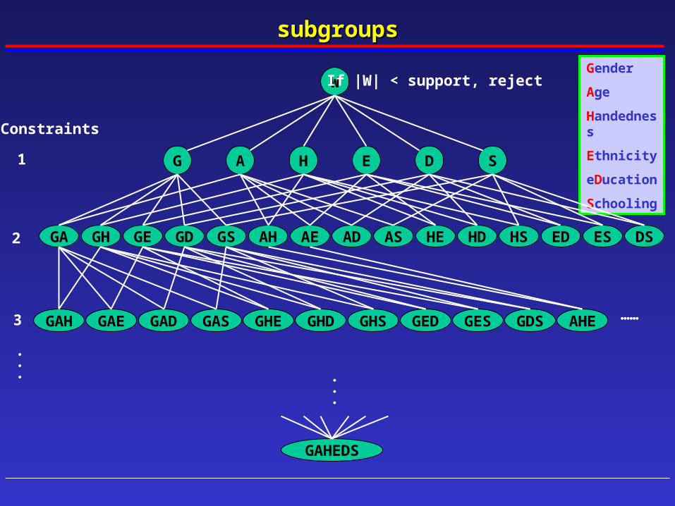
Gender

Age

Handedness

Ethnicity

eDucation

Schooling

G

W

SDEHA

If |W| < support, reject

Constraints

1

GA GH AH AE AD AS HE HD HS ED ES DSGSGDGE2

GAE GADGAH GAS GHE GHD GHS GED GES GDS AHE3 ……

.

.

.

GAHEDS

.

.

.

subgroupssubgroups

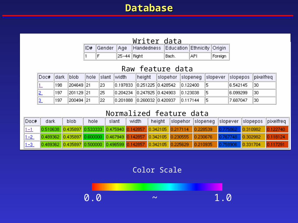
DatabaseDatabase

0.0 1.0~

Normalized feature data

Raw feature data

Writer data

Color Scale

Feature Database (White and Black)

12~24

25~44

45~64

>= 65

white black

Female

white black

Male

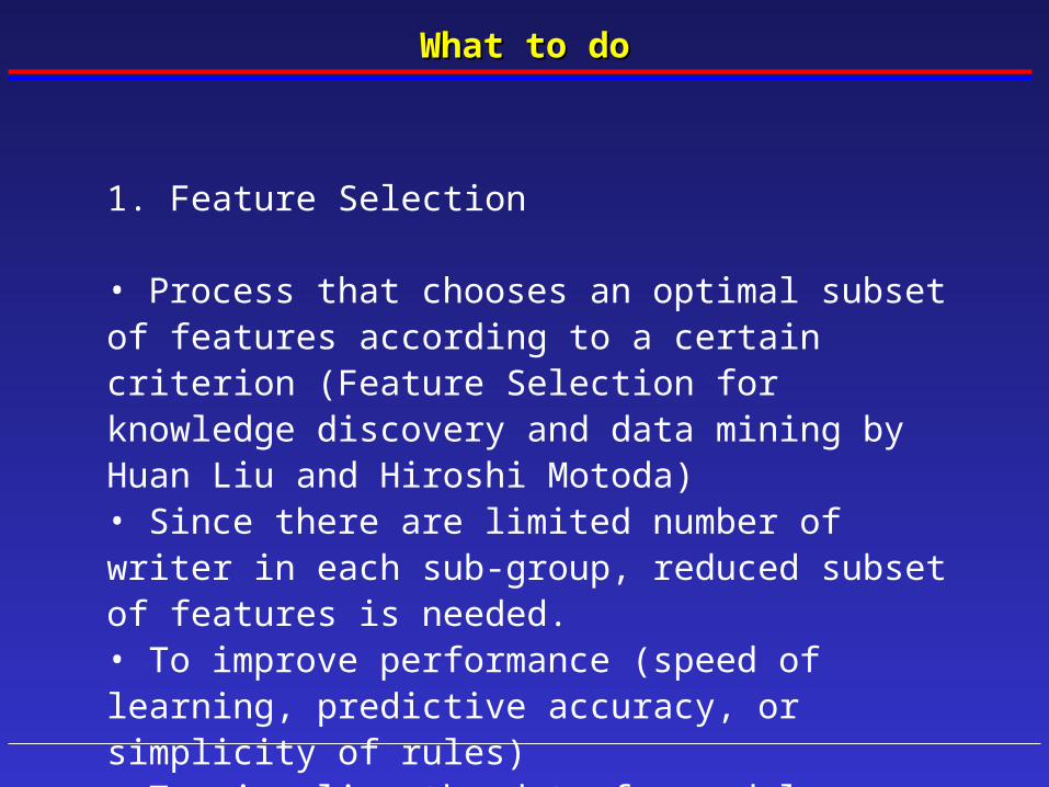
What to doWhat to do

1. Feature Selection

• Process that chooses an optimal subset of features according to a certain criterion (Feature Selection for knowledge discovery and data mining by Huan Liu and Hiroshi Motoda)• Since there are limited number of writer in each sub-group, reduced subset of features is needed. • To improve performance (speed of learning, predictive accuracy, or simplicity of rules)• To visualize the data for model selection• To reduce dimensionality and remove noise

Feature SelectionFeature Selection

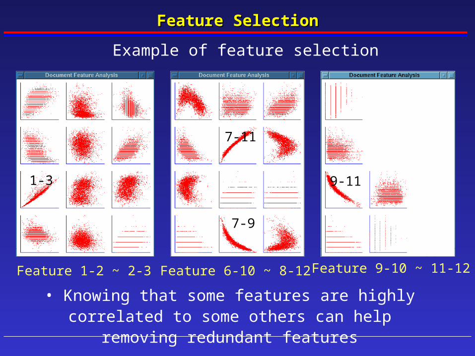
Example of feature selection

Feature 1-2 ~ 2-3 Feature 6-10 ~ 8-12

7-11

7-9

1-3

Feature 9-10 ~ 11-12

9-11

• Knowing that some features are highly correlated to some others can help removing redundant features

What to doWhat to do

2. Visualization of trend (if any) of writer sub-groups

• Useful tool so that we can quickly obtain an overall structural view of the trend of sub-group

• Seeing is Believing !

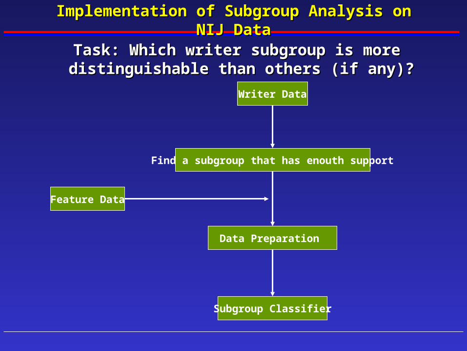
Implementation of Subgroup Analysis on NIJ DataImplementation of Subgroup Analysis on NIJ Data

Writer Data

Find a subgroup that has enouth support

Data Preparation

Subgroup Classifier

Feature Data

Task: Which writer subgroup is more Task: Which writer subgroup is more distinguishable than others (if any)?distinguishable than others (if any)?

The Result of Subgroup Classification ResultsThe Result of Subgroup Classification Results

Procedure for writer subgroup analysis

Find subgroup that has enough support Choose ‘the other’ (complement) groupMake data sets(4) for Artificial Neural NetworkTrain ANN and get the results from two test sets

Limit

3 categoris are used (gender, ethnicity and age)up to 2 constraints are consideredonly Document-level features are used

1

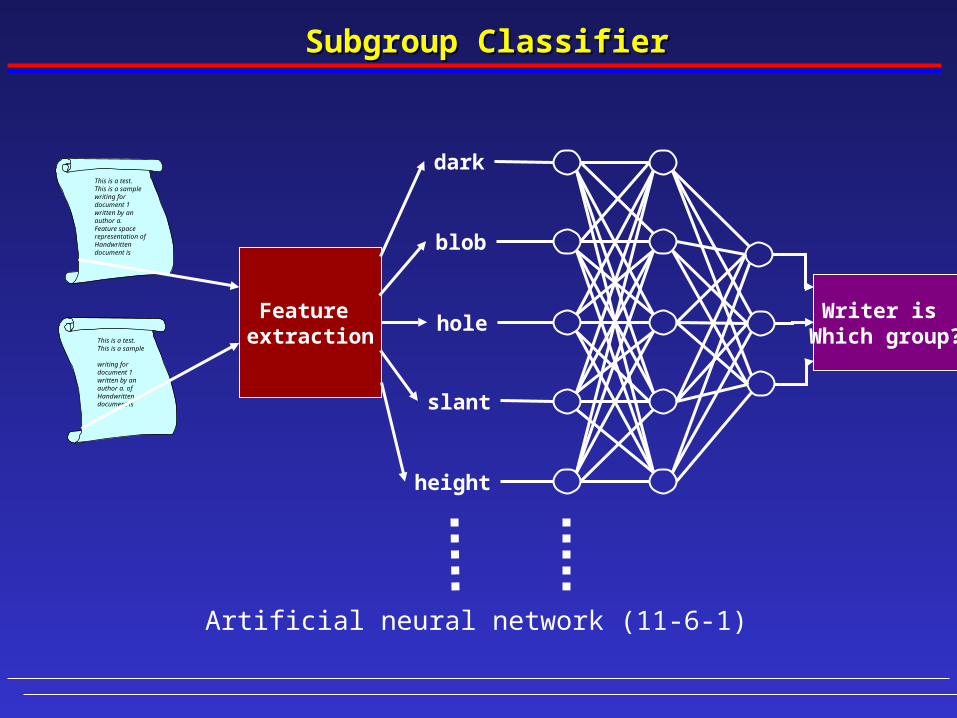
Subgroup ClassifierSubgroup Classifier

dark

blob

hole

slant

height

Artificial neural network (11-6-1)

This is a test.This is a sample writing fordocument 1 written by an author a.Feature space representation of Handwritten document is

This is a test.This is a sample

writing fordocument 1 written by an author a. of Handwritten document is

Feature extraction

Writer is Which group?

The Result of Subgroup Classification ResultsThe Result of Subgroup Classification Results

Error Rate (Test1) Error Rate (Test2) Average

Age1 25.6% 33.9% 29.8%Age2 31.5% 30.2% 30.9%Age3 44.9% 41.9% 43.4%Age4 28.7% 32.4% 30.6%Age5 19.1% 18.8% 19.0%White 29.8% 32.3% 31.1%Black 30.2% 31.7% 31.0%

Hispanic 25.2% 33.8% 29.5%Female2 32.4% 33.3% 32.9%Female3 30.0% 36.7% 33.4%Female4 25.5% 20.3% 22.9%Female5 15.0% 16.6% 15.8%

Female Black 29.7% 34.7% 32.2%Female White 32.6% 34.8% 33.7%

Male2 43.6% 31.9% 37.8%Male3 38.0% 40.0% 39.0%

Male White 32.7% 34.1% 33.4%

They’re distinguishable, but why...They’re distinguishable, but why...

• Need to explain why they’re distinguishable• ANN does a good job, but can’t explain clearly its output• 12 features are too many to explain and visualize• Only 2 (or 3) dimensions are visualizable• Question : Does a reasonable two or three dimensional representation of the data exist that may be analyzed visually?

Reference : Feature Selection for Knowledge Discovery and Data Mining

- Huan Liu and Hiroshi Motoda

Feature ExtractionFeature Extraction

• Common characteristic of feature extraction methods is that they all produce new features y based on the original features x.

• After feature extraction, representation of data is changed so that many techniques such as visualization, decision tree building can be conveniently used.

• Feature extraction started, as early as in 60’s and 70’s, as a problem of finding the intrinsic dimensionality of a data set - the minimum number of independent features required to generate the instances

Visualization PerspectiveVisualization Perspective

• Data of high dimensions cannot be analyzed visually

• It is often necessary to reduce it’s dimensionality in order to visualize the data

• The most popular method of determining topological dimensionality is the Karhunen-Loeve (K-L) method (also called Principal Component Analysis) which is based on the eigenvalues of a covariance matrix(R) computed from the data

Visualization PerspectiveVisualization Perspective

• The M eigenvectors corresponding to the M largest eigenvalues of R define a linear transformation from the N-dimensional space to an M-dimensional space in which the features are uncorrelated.

• This property of uncorrelated features is derived from a theorem stating that if the eigenvalues of a matrix are distinct, then the associated eigenvectors are linearly independent • For the purpose of visualization, one may take the M features corresponding to the M largest eigenvalues of R

Applied to the NIJ dataApplied to the NIJ data

1. Normalize each feature’s values into a range [0,1]2. Obtain the correlation matrix for the 12 original features3. Find eigenvalues of the correlation matrix4. Select the largest two eigenvalues should be chosen5. Output the chosen eigenvectors associated with the chosen eigenvalues. Here we obtain a 12 * 2 transformation matrix M6. Transform the normalized data Dold into data Dnew of

extracted features as follows:Dnew = Dold M

The resulting data is of 2-dimensional having the original class label attached to each instance

Applied to the NIJ dataApplied to the NIJ data

Applied to the NIJ dataApplied to the NIJ data

Sample Iris data (the original is 4-dimensional)