DATA MINING LECTURE 8 Clustering The k-means algorithm Hierarchical Clustering The DBSCAN algorithm.

DATA MININGLECTURE 8Clustering

The k-means algorithm

Hierarchical Clustering

The DBSCAN algorithm

What is a Clustering?• In general a grouping of objects such that the objects in a

group (cluster) are similar (or related) to one another and different from (or unrelated to) the objects in other groups

Inter-cluster distances are maximized

Intra-cluster distances are

minimized

Applications of Cluster Analysis

• Understanding• Group related documents for

browsing, genes and proteins that have similar functionality, stocks with similar price fluctuations, users with same behavior

• Summarization• Reduce the size of large data

sets

• Applications• Recommendation systems• Search Personalization

Discovered Clusters Industry Group

1 Applied-Matl-DOWN,Bay-Network-Down,3-COM-DOWN,

Cabletron-Sys-DOWN,CISCO-DOWN,HP-DOWN, DSC-Comm-DOWN,INTEL-DOWN,LSI-Logic-DOWN,

Micron-Tech-DOWN,Texas-Inst-Down,Tellabs-Inc-Down, Natl-Semiconduct-DOWN,Oracl-DOWN,SGI-DOWN,

Sun-DOWN

Technology1-DOWN

2 Apple-Comp-DOWN,Autodesk-DOWN,DEC-DOWN,

ADV-Micro-Device-DOWN,Andrew-Corp-DOWN, Computer-Assoc-DOWN,Circuit-City-DOWN,

Compaq-DOWN, EMC-Corp-DOWN, Gen-Inst-DOWN, Motorola-DOWN,Microsoft-DOWN,Scientific-Atl-DOWN

Technology2-DOWN

3 Fannie-Mae-DOWN,Fed-Home-Loan-DOWN, MBNA-Corp-DOWN,Morgan-Stanley-DOWN

Financial-DOWN

4 Baker-Hughes-UP,Dresser-Inds-UP,Halliburton-HLD-UP,

Louisiana-Land-UP,Phillips-Petro-UP,Unocal-UP, Schlumberger-UP

Oil-UP

Clustering precipitation in Australia

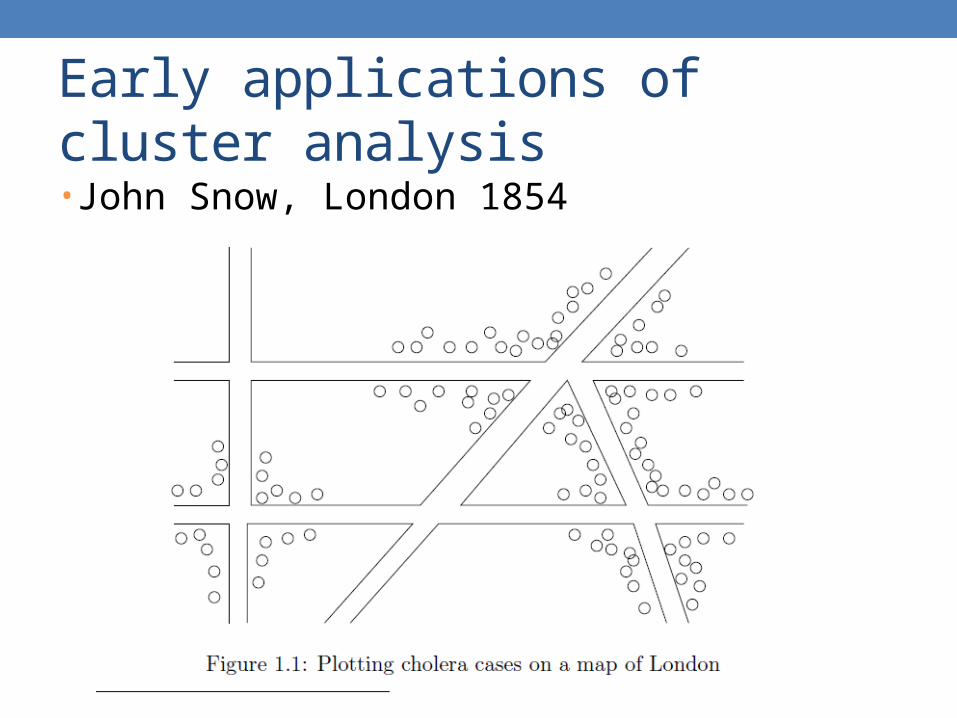
Early applications of cluster analysis

• John Snow, London 1854

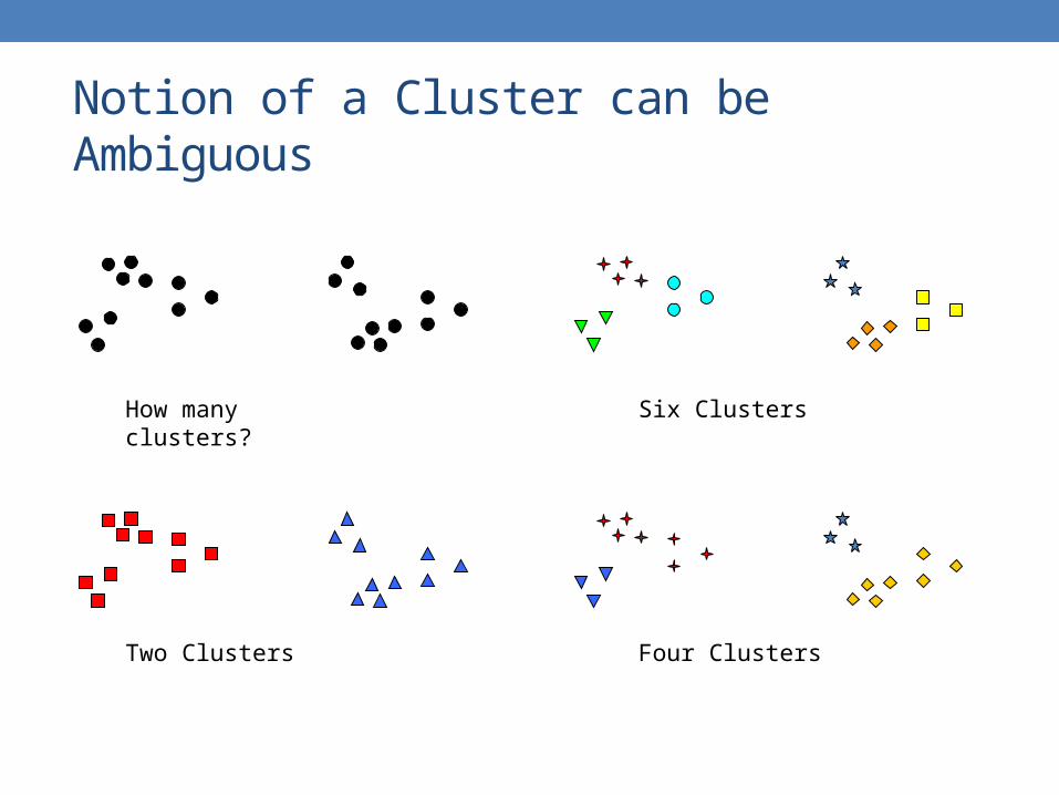
Notion of a Cluster can be Ambiguous

How many clusters?

Four Clusters Two Clusters

Six Clusters

Types of Clusterings

• A clustering is a set of clusters

• Important distinction between hierarchical and partitional sets of clusters

• Partitional Clustering• A division data objects into subsets (clusters) such

that each data object is in exactly one subset

• Hierarchical clustering• A set of nested clusters organized as a hierarchical

tree

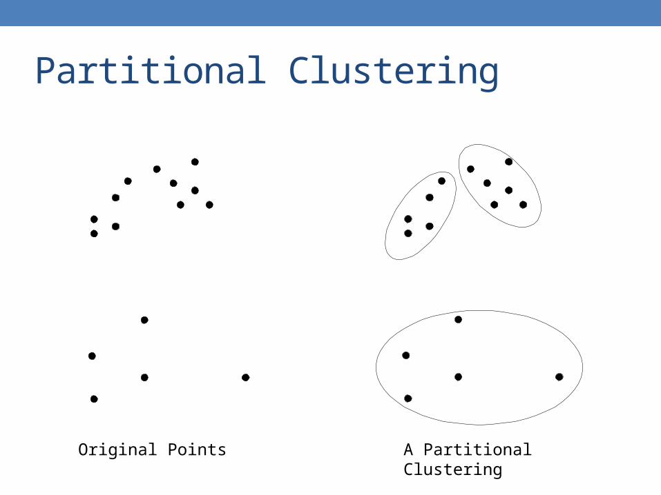
Partitional Clustering

Original Points A Partitional Clustering


p4p1

p3

p2

p4 p1

p3

p2

p4p1 p2 p3

p4p1 p2 p3

Traditional Hierarchical Clustering

Non-traditional Hierarchical Clustering

Non-traditional Dendrogram

Traditional Dendrogram

Other types of clustering• Exclusive (or non-overlapping) versus non-

exclusive (or overlapping) • In non-exclusive clusterings, points may belong to

multiple clusters.• Points that belong to multiple classes, or ‘border’ points

• Fuzzy (or soft) versus non-fuzzy (or hard)• In fuzzy clustering, a point belongs to every cluster

with some weight between 0 and 1• Weights usually must sum to 1 (often interpreted as probabilities)

• Partial versus complete• In some cases, we only want to cluster some of the

data

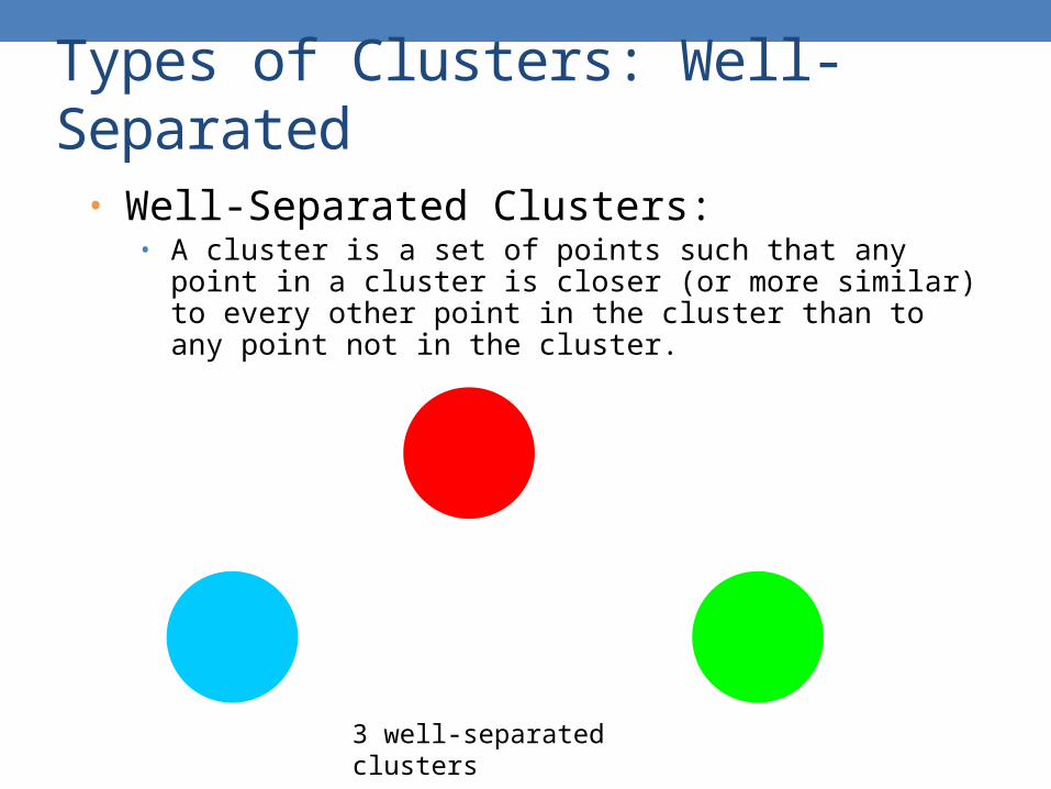
Types of Clusters: Well-Separated

• Well-Separated Clusters: • A cluster is a set of points such that any point in a cluster is

closer (or more similar) to every other point in the cluster than to any point not in the cluster.

3 well-separated clusters

Types of Clusters: Center-Based

• Center-based• A cluster is a set of objects such that an object in a cluster is

closer (more similar) to the “center” of a cluster, than to the center of any other cluster

• The center of a cluster is often a centroid, the minimizer of distances from all the points in the cluster, or a medoid, the most “representative” point of a cluster

4 center-based clusters

Types of Clusters: Contiguity-Based

• Contiguous Cluster (Nearest neighbor or Transitive)• A cluster is a set of points such that a point in a cluster is

closer (or more similar) to one or more other points in the cluster than to any point not in the cluster.

8 contiguous clusters

Types of Clusters: Density-Based

• Density-based• A cluster is a dense region of points, which is separated by

low-density regions, from other regions of high density. • Used when the clusters are irregular or intertwined, and when

noise and outliers are present.

6 density-based clusters

Types of Clusters: Conceptual Clusters

• Shared Property or Conceptual Clusters• Finds clusters that share some common property or represent

a particular concept. .

2 Overlapping Circles

Types of Clusters: Objective Function

• Clustering as an optimization problem• Finds clusters that minimize or maximize an objective function. • Enumerate all possible ways of dividing the points into clusters

and evaluate the `goodness' of each potential set of clusters by using the given objective function. (NP Hard)

• Can have global or local objectives.• Hierarchical clustering algorithms typically have local objectives• Partitional algorithms typically have global objectives

• A variation of the global objective function approach is to fit the data to a parameterized model. • The parameters for the model are determined from the data, and they

determine the clustering• E.g., Mixture models assume that the data is a ‘mixture' of a number of

statistical distributions.

Clustering Algorithms

• K-means and its variants

• Hierarchical clustering

• DBSCAN

K-MEANS

K-means Clustering

• Partitional clustering approach • Each cluster is associated with a centroid

(center point) • Each point is assigned to the cluster with the

closest centroid• Number of clusters, K, must be specified• The objective is to minimize the sum of

distances of the points to their respective centroid

K-means Clustering

• Problem: Given a set X of n points in a d-dimensional space and an integer K group the points into K clusters C= {C1, C2,…,Ck} such that

is minimized, where ci is the centroid of the points in cluster Ci

K-means Clustering

• Most common definition is with euclidean distance, minimizing the Sum of Squares Error (SSE) function• Sometimes K-means is defined like that

• Problem: Given a set X of n points in a d-dimensional space and an integer K group the points into K clusters C= {C1, C2,…,Ck} such that

is minimized, where ci is the mean of the points in cluster Ci

Sum of Squares Error (SSE)

Complexity of the k-means problem

• NP-hard if the dimensionality of the data is at least 2 (d≥2)• Finding the best solution in polynomial time is infeasible

• For d=1 the problem is solvable in polynomial time (how?)

• A simple iterative algorithm works quite well in practice

K-means Algorithm

• Also known as Lloyd’s algorithm.• K-means is sometimes synonymous with this algorithm

K-means Algorithm – Initialization

• Initial centroids are often chosen randomly.• Clusters produced vary from one run to another.

Two different K-means Clusterings

-2 -1.5 -1 -0.5 0 0.5 1 1.5 2

0

0.5

1

1.5

2

2.5

3

x

y

-2 -1.5 -1 -0.5 0 0.5 1 1.5 2

0

0.5

1

1.5

2

2.5

3

x

y

Sub-optimal Clustering

-2 -1.5 -1 -0.5 0 0.5 1 1.5 2

0

0.5

1

1.5

2

2.5

3

x

y

Optimal Clustering

Original Points

Importance of Choosing Initial Centroids

-2 -1.5 -1 -0.5 0 0.5 1 1.5 2

0

0.5

1

1.5

2

2.5

3

x

y

Iteration 1

-2 -1.5 -1 -0.5 0 0.5 1 1.5 2

0

0.5

1

1.5

2

2.5

3

x

y

Iteration 2

-2 -1.5 -1 -0.5 0 0.5 1 1.5 2

0

0.5

1

1.5

2

2.5

3

x

y

Iteration 3

-2 -1.5 -1 -0.5 0 0.5 1 1.5 2

0

0.5

1

1.5

2

2.5

3

x

y

Iteration 4

-2 -1.5 -1 -0.5 0 0.5 1 1.5 2

0

0.5

1

1.5

2

2.5

3

x

y

Iteration 5

-2 -1.5 -1 -0.5 0 0.5 1 1.5 2

0

0.5

1

1.5

2

2.5

3

x

y

Iteration 6

Importance of Choosing Initial Centroids

-2 -1.5 -1 -0.5 0 0.5 1 1.5 2

0

0.5

1

1.5

2

2.5

3

x

y

Iteration 1

-2 -1.5 -1 -0.5 0 0.5 1 1.5 2

0

0.5

1

1.5

2

2.5

3

x

y

Iteration 2

-2 -1.5 -1 -0.5 0 0.5 1 1.5 2

0

0.5

1

1.5

2

2.5

3

x

y

Iteration 3

-2 -1.5 -1 -0.5 0 0.5 1 1.5 2

0

0.5

1

1.5

2

2.5

3

x

y

Iteration 4

-2 -1.5 -1 -0.5 0 0.5 1 1.5 2

0

0.5

1

1.5

2

2.5

3

x

y

Iteration 5

Importance of Choosing Initial Centroids …

-2 -1.5 -1 -0.5 0 0.5 1 1.5 2

0

0.5

1

1.5

2

2.5

3

x

yIteration 1

-2 -1.5 -1 -0.5 0 0.5 1 1.5 2

0

0.5

1

1.5

2

2.5

3

x

y

Iteration 2

-2 -1.5 -1 -0.5 0 0.5 1 1.5 2

0

0.5

1

1.5

2

2.5

3

x

y

Iteration 3

-2 -1.5 -1 -0.5 0 0.5 1 1.5 2

0

0.5

1

1.5

2

2.5

3

x

y

Iteration 4

-2 -1.5 -1 -0.5 0 0.5 1 1.5 2

0

0.5

1

1.5

2

2.5

3

x

y

Iteration 5

Dealing with Initialization

• Do multiple runs and select the clustering with the smallest error

• Select original set of points by methods other than random . E.g., pick the most distant (from each other) points as cluster centers (K-means++ algorithm)

K-means Algorithm – Centroids• The centroid depends on the distance function

• The minimizer for the distance function

• ‘Closeness’ is measured by Euclidean distance (SSE), cosine similarity, correlation, etc.

• Centroid:• The mean of the points in the cluster for SSE, and cosine

similarity• The median for Manhattan distance.

• Finding the centroid is not always easy • It can be an NP-hard problem for some distance functions

• E.g., median form multiple dimensions

K-means Algorithm – Convergence

• K-means will converge for common similarity measures mentioned above.• Most of the convergence happens in the first few

iterations.• Often the stopping condition is changed to ‘Until

relatively few points change clusters’

• Complexity is O( n * K * I * d )• n = number of points, K = number of clusters,

I = number of iterations, d = dimensionality

• In general a fast and efficient algorithm

Limitations of K-means

• K-means has problems when clusters are of different • Sizes• Densities• Non-globular shapes

• K-means has problems when the data contains outliers.

Limitations of K-means: Differing Sizes

Original Points K-means (3 Clusters)

Limitations of K-means: Differing Density


Limitations of K-means: Non-globular Shapes


Overcoming K-means Limitations

Original Points K-means Clusters

One solution is to use many clusters.Find parts of clusters, but need to put together.

Overcoming K-means Limitations

Original Points K-means Clusters

Variations

• K-medoids: Similar problem definition as in K-means, but the centroid of the cluster is defined to be one of the points in the cluster (the medoid).

• K-centers: Similar problem definition as in K-means, but the goal now is to minimize the maximum diameter of the clusters (diameter of a cluster is maximum distance between any two points in the cluster).

HIERARCHICAL CLUSTERING

Hierarchical Clustering• Two main types of hierarchical clustering

• Agglomerative: • Start with the points as individual clusters• At each step, merge the closest pair of clusters until only one cluster (or

k clusters) left

• Divisive: • Start with one, all-inclusive cluster • At each step, split a cluster until each cluster contains a point (or there

are k clusters)

• Traditional hierarchical algorithms use a similarity or distance matrix• Merge or split one cluster at a time


• Produces a set of nested clusters organized as a hierarchical tree

• Can be visualized as a dendrogram• A tree like diagram that records the sequences of

merges or splits

1 3 2 5 4 60

0.05

0.1

0.15

0.2

1

2

3

4

5

6

1

23 4

5

Strengths of Hierarchical Clustering• Do not have to assume any particular number of clusters• Any desired number of clusters can be obtained by

‘cutting’ the dendogram at the proper level

• They may correspond to meaningful taxonomies• Example in biological sciences (e.g., animal kingdom,

phylogeny reconstruction, …)

Agglomerative Clustering Algorithm• More popular hierarchical clustering technique

• Basic algorithm is straightforward1. Compute the proximity matrix2. Let each data point be a cluster3. Repeat4. Merge the two closest clusters5. Update the proximity matrix6. Until only a single cluster remains

• Key operation is the computation of the proximity of two clusters

• Different approaches to defining the distance between clusters distinguish the different algorithms

Starting Situation • Start with clusters of individual points and a proximity matrix

p1

p3

p5

p4

p2

p1 p2 p3 p4 p5 . . .

.

.

. Proximity Matrix

...p1 p2 p3 p4 p9 p10 p11 p12

Intermediate Situation• After some merging steps, we have some clusters

C1

C4

C2 C5

C3

C2C1

C1

C3

C5

C4

C2

C3 C4 C5

Proximity Matrix

...p1 p2 p3 p4 p9 p10 p11 p12

Intermediate Situation• We want to merge the two closest clusters (C2 and C5) and

update the proximity matrix.

C1

C4

C2 C5

C3

C2C1

C1

C3

C5

C4

C2

C3 C4 C5

Proximity Matrix

...p1 p2 p3 p4 p9 p10 p11 p12

After Merging• The question is “How do we update the proximity matrix?”

C1

C4

C2 U C5

C3 ? ? ? ?

?

?

?

C2 U C5C1

C1

C3

C4

C2 U C5

C3 C4

Proximity Matrix

...p1 p2 p3 p4 p9 p10 p11 p12

How to Define Inter-Cluster Similarity

p1

p3

p5

p4

p2

p1 p2 p3 p4 p5 . . .

.

.

.

Similarity?

MIN MAX Group Average Distance Between Centroids Other methods driven by an objective

function– Ward’s Method uses squared error

Proximity Matrix

How to Define Inter-Cluster Similarity

p1

p3

p5

p4

p2

p1 p2 p3 p4 p5 . . .

.

.

.Proximity Matrix

MIN MAX Group Average Distance Between Centroids Other methods driven by an objective

function– Ward’s Method uses squared error

Single Link – Complete Link

• Another way to view the processing of the hierarchical algorithm is that we create links between the elements in order of increasing distance• The MIN – Single Link, will merge two clusters when a

single pair of elements is linked• The MAX – Complete Linkage will merge two clusters

when all pairs of elements have been linked.

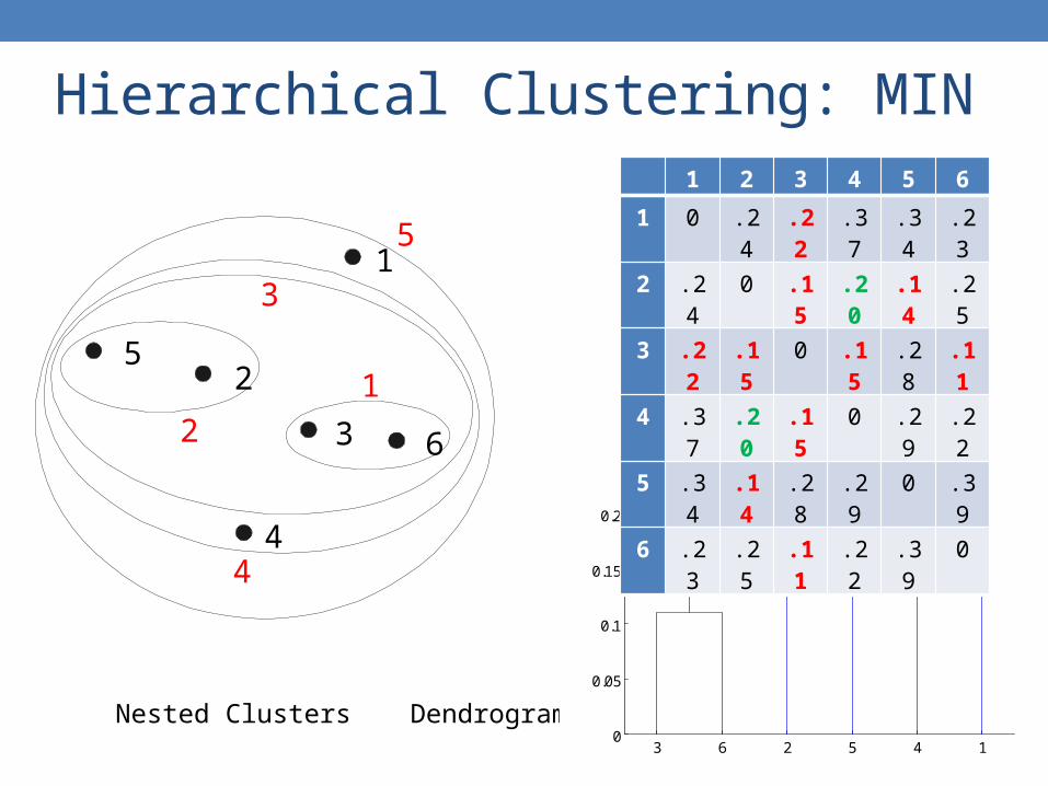
Hierarchical Clustering: MIN

Nested Clusters Dendrogram

1

2

3

4

5

6

1

2

3

4

5

3 6 2 5 4 10

0.05

0.1

0.15

0.2

1 2 3 4 5 6

1 0 .24 .22 .37 .34 .23

2 .24 0 .15 .20 .14 .25

3 .22 .15 0 .15 .28 .11

4 .37 .20 .15 0 .29 .22

5 .34 .14 .28 .29 0 .39

6 .23 .25 .11 .22 .39 0

1 2 3 4 5 6

1 0 .24 .22 .37 .34 .23

2 .24 0 .15 .20 .14 .25

3 .22 .15 0 .15 .28 .11

4 .37 .20 .15 0 .29 .22

5 .34 .14 .28 .29 0 .39

6 .23 .25 .11 .22 .39 0

1 2 3 4 5 6

1 0 .24 .22 .37 .34 .23

2 .24 0 .15 .20 .14 .25

3 .22 .15 0 .15 .28 .11

4 .37 .20 .15 0 .29 .22

5 .34 .14 .28 .29 0 .39

6 .23 .25 .11 .22 .39 0

1 2 3 4 5 6

1 0 .24 .22 .37 .34 .23

2 .24 0 .15 .20 .14 .25

3 .22 .15 0 .15 .28 .11

4 .37 .20 .15 0 .29 .22

5 .34 .14 .28 .29 0 .39

6 .23 .25 .11 .22 .39 0

1 2 3 4 5 6

1 0 .24 .22 .37 .34 .23

2 .24 0 .15 .20 .14 .25

3 .22 .15 0 .15 .28 .11

4 .37 .20 .15 0 .29 .22

5 .34 .14 .28 .29 0 .39

6 .23 .25 .11 .22 .39 0

1 2 3 4 5 6

1 0 .24 .22 .37 .34 .23

2 .24 0 .15 .20 .14 .25

3 .22 .15 0 .15 .28 .11

4 .37 .20 .15 0 .29 .22

5 .34 .14 .28 .29 0 .39

6 .23 .25 .11 .22 .39 0

Strength of MIN

Original Points Two Clusters

• Can handle non-elliptical shapes

Limitations of MIN


• Sensitive to noise and outliers

Hierarchical Clustering: MAX


3 6 4 1 2 50

0.05

0.1

0.15

0.2

0.25

0.3

0.35

0.4

1

2

3

4

5

6

1

2 5

3

4

1 2 3 4 5 6

1 0 .24 .22 .37 .34 .23

2 .24 0 .15 .20 .14 .25

3 .22 .15 0 .15 .28 .11

4 .37 .20 .15 0 .29 .22

5 .34 .14 .28 .29 0 .39

6 .23 .25 .11 .22 .39 0

1 2 3 4 5 6

1 0 .24 .22 .37 .34 .23

2 .24 0 .15 .20 .14 .25

3 .22 .15 0 .15 .28 .11

4 .37 .20 .15 0 .29 .22

5 .34 .14 .28 .29 0 .39

6 .23 .25 .11 .22 .39 0

1 2 3 4 5 6

1 0 .24 .22 .37 .34 .23

2 .24 0 .15 .20 .14 .25

3 .22 .15 0 .15 .28 .11

4 .37 .20 .15 0 .29 .22

5 .34 .14 .28 .29 0 .39

6 .23 .25 .11 .22 .39 0

1 2 3 4 5 6

1 0 .24 .22 .37 .34 .23

2 .24 0 .15 .20 .14 .25

3 .22 .15 0 .15 .28 .11

4 .37 .20 .15 0 .29 .22

5 .34 .14 .28 .29 0 .39

6 .23 .25 .11 .22 .39 0

1 2 3 4 5 6

1 0 .24 .22 .37 .34 .23

2 .24 0 .15 .20 .14 .25

3 .22 .15 0 .15 .28 .11

4 .37 .20 .15 0 .29 .22

5 .34 .14 .28 .29 0 .39

6 .23 .25 .11 .22 .39 0

Strength of MAX


• Less susceptible to noise and outliers

Limitations of MAX


•Tends to break large clusters

•Biased towards globular clusters

Cluster Similarity: Group Average• Proximity of two clusters is the average of pairwise proximity

between points in the two clusters.

• Need to use average connectivity for scalability since total proximity favors large clusters

||Cluster||Cluster

)p,pproximity(

)Cluster,Clusterproximity(ji

ClusterpClusterp

ji

jijjii

1 2 3 4 5 6

1 0 .24 .22 .37 .34 .23

2 .24 0 .15 .20 .14 .25

3 .22 .15 0 .15 .28 .11

4 .37 .20 .15 0 .29 .22

5 .34 .14 .28 .29 0 .39

6 .23 .25 .11 .22 .39 0

Hierarchical Clustering: Group Average


3 6 4 1 2 50

0.05

0.1

0.15

0.2

0.25

1

2

3

4

5

6

1

2

5

3

4

1 2 3 4 5 6

1 0 .24 .22 .37 .34 .23

2 .24 0 .15 .20 .14 .25

3 .22 .15 0 .15 .28 .11

4 .37 .20 .15 0 .29 .22

5 .34 .14 .28 .29 0 .39

6 .23 .25 .11 .22 .39 0

Hierarchical Clustering: Group Average

• Compromise between Single and Complete Link

• Strengths• Less susceptible to noise and outliers

• Limitations• Biased towards globular clusters

Cluster Similarity: Ward’s Method

• Similarity of two clusters is based on the increase in squared error (SSE) when two clusters are merged• Similar to group average if distance between points is

distance squared

• Less susceptible to noise and outliers

• Biased towards globular clusters

• Hierarchical analogue of K-means• Can be used to initialize K-means

Hierarchical Clustering: Comparison

Group Average

Ward’s Method

1

2

3

4

5

61

2

5

3

4

MIN MAX

1

2

3

4

5

61

2

5

34

1

2

3

4

5

61

2 5

3

41

2

3

4

5

6

12

3

4

5

Hierarchical Clustering: Time and Space requirements

• O(N2) space since it uses the proximity matrix. • N is the number of points.

• O(N3) time in many cases• There are N steps and at each step the size, N2,

proximity matrix must be updated and searched• Complexity can be reduced to O(N2 log(N) ) time for

some approaches

Hierarchical Clustering: Problems and Limitations• Computational complexity in time and space

• Once a decision is made to combine two clusters, it cannot be undone

• No objective function is directly minimized

• Different schemes have problems with one or more of the following:• Sensitivity to noise and outliers• Difficulty handling different sized clusters and convex shapes• Breaking large clusters

DBSCAN

DBSCAN: Density-Based Clustering• DBSCAN is a Density-Based Clustering algorithm

• Reminder: In density based clustering we partition points into dense regions separated by not-so-dense regions.

• Important Questions:• How do we measure density?• What is a dense region?

• DBSCAN:• Density at point p: number of points within a circle of radius Eps• Dense Region: A circle of radius Eps that contains at least MinPts

points

DBSCAN• Characterization of points

• A point is a core point if it has more than a specified number of points (MinPts) within Eps• These points belong in a dense region and are at the interior

of a cluster

• A border point has fewer than MinPts within Eps, but is in the neighborhood of a core point.

• A noise point is any point that is not a core point or a border point.

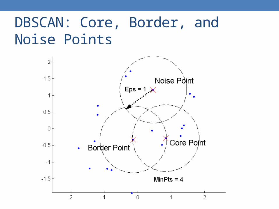
DBSCAN: Core, Border, and Noise Points

DBSCAN: Core, Border and Noise Points

Original PointsPoint types: core, border and noise

Eps = 10, MinPts = 4

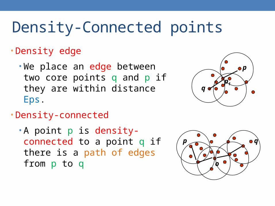
Density-Connected points• Density edge

• We place an edge between two core points q and p if they are within distance Eps.

• Density-connected

• A point p is density-connected to a point q if there is a path of edges from p to q

p

qp1

p q

o

DBSCAN Algorithm

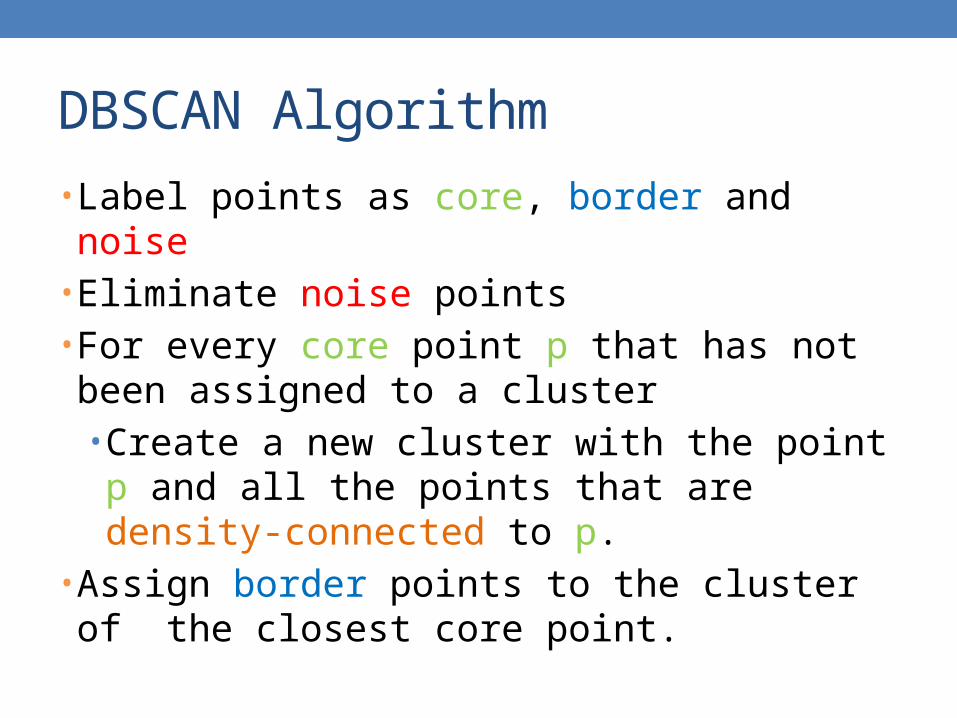
• Label points as core, border and noise• Eliminate noise points• For every core point p that has not been assigned to a cluster• Create a new cluster with the point p and all the points that are density-connected to p.

• Assign border points to the cluster of the closest core point.

DBSCAN: Determining Eps and MinPts• Idea is that for points in a cluster, their kth nearest neighbors are

at roughly the same distance• Noise points have the kth nearest neighbor at farther distance• So, plot sorted distance of every point to its kth nearest neighbor• Find the distance d where there is a “knee” in the curve

• Eps = d, MinPts = k

Eps ~ 7-10MinPts = 4

When DBSCAN Works Well

Original PointsClusters

• Resistant to Noise

• Can handle clusters of different shapes and sizes

When DBSCAN Does NOT Work Well

Original Points

(MinPts=4, Eps=9.75).

(MinPts=4, Eps=9.92)

• Varying densities

• High-dimensional data

DBSCAN: Sensitive to Parameters

Other algorithms• PAM, CLARANS: Solutions for the k-medoids problem• BIRCH: Constructs a hierarchical tree that acts a

summary of the data, and then clusters the leaves.• MST: Clustering using the Minimum Spanning Tree.• ROCK: clustering categorical data by neighbor and link

analysis• LIMBO, COOLCAT: Clustering categorical data using

information theoretic tools.• CURE: Hierarchical algorithm uses different

representation of the cluster• CHAMELEON: Hierarchical algorithm uses closeness and

interconnectivity for merging

DATA MINING LECTURE 8 Clustering The k-means algorithm Hierarchical Clustering The DBSCAN algorithm.

Documents

Transcript of DATA MINING LECTURE 8 Clustering The k-means algorithm Hierarchical Clustering The DBSCAN algorithm.