Data Mining in Forecasting PVT Correlations of Crude Oil Systems Based on Type-1 Fuzzy Logic Inference

Systems

1

2

3

4

5 6

Emad A. El-Sebakhy Information & Computer Science Department, College of Computer Sciences and Engineering,

King Fahd University of Petroleum & Minerals, Dhahran 31261, Saudi Arabia sebakhy@kfupm.edu.sa and eae6@cornell.edu 7

Abstract 8

9

10

11

12

13

14

15

16

17

18

19

20

21

22

23

24

25

26

Pressure-Volume-Temperature properties are very important in the reservoir engineering computations. There are many

empirical approaches for predicting various PVT properties using regression models. Last decade, researchers utilized neural

networks to develop more accurate PVT correlations. These achievements of neural networks open the door to data mining

techniques to play a major role in oil and gas industry. Unfortunately, the developed neural networks correlations are often

limited and global correlations are usually less accurate compared to local correlations. Recently, adaptive neuro-fuzzy

inference systems have been proposed as a new intelligence framework for both prediction and classification based on fuzzy

clustering optimization criterion and ranking. This paper proposes neuro-fuzzy inference systems for estimating PVT properties

of crude oil systems. This new framework is an efficient tool for modeling the kind of uncertainty associated with vagueness and

imprecision. It is a novel hybrid computational intelligence scheme that is able to forecast/classify an output in the uncertainty

situations. We briefly describe the learning steps and the use of the Takagi Sugeno and Kang model and Gustafson–Kessel

clustering algorithm with K-detected clusters from the given database. It has featured in a wide range of medical, power control

system, and business journals, often with promising results. A comparative study will be carried out to compare their

performance of this new framework with the most popular modeling techniques, such as, neural networks, nonlinear regression,

and the empirical correlations algorithms. The results show that the performance of neuro-fuzzy systems is accurate, reliable,

and outperform most of the existing forecasting techniques. Future work can be achieved by using neuro fuzzy systems for

clustering the 3D seismic data, identification of lithofacies types, and other reservoir characterization.

Keywords –Type1 neuro-fuzzy systems; Feedforward neural networks, Empirical correlations, PVT properties; Formation

volume factor; Bubble point pressure

1

1. Introduction 1

2

3

4

5

6

7

8

9

10

11

12

13

14

15

16

17

18

19

20

21

22

23

24

25

26

27

Knowing both chemical and physical properties of formation water is very important in various reservoir

engineering computations, especially in water flooding and production. Ideally, these properties should be obtained

experimentally. On some occasions, these properties are neither available nor reliable; then, empirically derived

correlations are used to predict brine Pressure-Volume-Temperature (PVT) properties. These correlations offer an

acceptable approximation of formation water properties. However, the success of such correlations in prediction

depends mainly on the range of data at which they were originally developed. These correlations were developed

using equation of state (EOS), linear/nonlinear statistical regression, or graphical techniques. The currently available

PVT simulator predicts the physical properties of reservoir fluids with vary degree of accuracy based on the type of

used model, the nature of fluid, and the prevailing conditions. Nevertheless, they all exhibit the significant

drawback of lacking the ability to forecast the quality of their answers. The equation of state is based on knowing

the detailed compositions of the reservoir fluids. The determination of such quantities is expensive and time

consuming.

The equation of state involves numerous numerical computations. On the other hand, PVT correlations are

based on easily measured field data: reservoir pressure, reservoir temperature, oil, and gas specific gravity. In the

petroleum process industries, reliable experimental data are always to be preferred over data obtained from

correlations. However, very often reliable experimental data are not available, and the advantage of a correlation is

that it may be used to predict properties for which very little experimental information is available. The importance

of accurate PVT data for material-balance calculations is well understood. It is crucial that all calculations in

reservoir performance, in production operations and design, and in formation evaluation be as good as the PVT

properties used in these calculations. The economics of the process also depends on the accuracy of such properties.

Reservoir fluid properties are very important in petroleum engineering computations, such as, material balance

calculations, well test analysis, reserve estimates, inflow performance calculations, and numerical reservoir

simulations. Ideally, these properties are determined from laboratory studies on samples collected from the bottom

of the wellbore or at the surface. Such experimental data are, however, very costly to obtain. Therefore, the

solution is to use the empirically derived correlations to predict PVT properties, see Osman et al. (2001). There are

many empirical correlations for predicting PVT properties, most of them were developed using equations of state

2

(EOS) or linear/non-linear multiple regression or graphical techniques or feedforward neural networks (FFN).

However, they often do not perform very accurately and suffer from a number of drawbacks, such as, FFN is a

black box modeling scheme that is based on the trial-and-error approach. In addition, FFN architectural parameters

have to be guessed in advance, such as, number and size of hidden layers and the type of transfer function(s) for

neurons in the various layers. Moreover, the training algorithm parameters were determined based on guessing

initial random weights, learning rate, and momentum. Although acceptable results may be obtained with effort, it is

obvious that potentially superior models can be overlooked.

1

2

3

4

5

6

7

8

9

10

11

12

13

14

15

16

17

18

19

20

21

22

23

24

25

26

The considerable amount of user intervention not only slows down model development, but also works against

the principle of ‘letting the data speak’. Furthermore, each correlation was developed for a certain range of

reservoir fluid characteristics and geographical area with similar fluid compositions and API oil gravity. Thus, the

accuracy of such correlations is critical and not often known in advance. Among those PVT properties is the bubble

point pressure (Pb), Oil Formation Volume Factor (Bob), which is defined as the volume of reservoir oil that would

be occupied by one stock tank barrel oil plus any dissolved gas at the bubble point pressure and reservoir

temperature. Precise prediction of Bo is very important in reservoir and production computations.

The development of correlations for PVT calculations has been the subject of extensive research, resulting in a

large volume of publications. Several graphical and mathematical correlations for determining both Pb and Bo have

been proposed during the last decade. These correlations are essentially based on the assumption that Pb and Bo are

strong functions of the solution gas-oil ratio (Rs), the reservoir temperature (Tf), the gas specific gravity (Gg), and

the oil specific gravity (G0), see El-Sebakhy et al. (2007), Goda et al. (2003), and Osman et al. (2001) for more

details.

The main objective of this paper is to investigate the feasibility of Type1 neuro fuzzy inference systems

(ANFIS) in estimating the PVT properties of crude oil systems, specifically develop a new intelligence system

framework for predicting both bubble point pressure and Oil Formation Volume Factor using different databases of

four input parameters, namely, solution gas-oil ratio (Rs), reservoir temperature (Tf), oil gravity (API), and gas

relative density. The rest of this paper is organized as follows. Section 2 provides a brief literature review and

related work. Section 3 provides both data acquisition and statistical quality measures. Section 4 consists of the

3

1

2

3

4

5

6

7

8

9

10

11

12

13

14

15

16

17

18

19

20

21

22

23

24

25

adaptive neuro-fuzzy inference systems methodology and architecture. The experimental set-up is discussed in

section 5. Section 6 shows the performance of the approach by giving the experimental results.

2. Literature Review

Last six decades, engineers realized the importance of developing and using empirical correlations for PVT

properties. Studies carried out in this field resulted in the development of new correlations.

2.1. Empirical Models and Evaluation Studies

There are numerous of empirical correlations published in literature, the most popular ones can be summarized

as, (a) in 1947, the author in Standing (1947) presented Standing empirical correlations for bubble point pressure

and for oil formation volume factor. These empirical correlations were based on laboratory experiments carried out

on 105 samples from 22 different crude oils in California, (b) in 1980, Glazo (1980) developed Glaso empirical

correlation for formation volume factor using 45 oil samples from North Sea hydrocarbon mixtures, and (c) in 1992,

the author in Al-Marhoun (1992) published his second Al-Marhoun empirical correlation for oil formation volume

factor based on database of 11,728 experimentally data points for formation volume factors at, above, and below

bubble point pressure. The data set represents samples from more than 700 reservoirs from all over the world,

mostly from Middle East and North America. The reader can consider other empirical correlations, see Al-

Shammasi (1997) and El-Sebakhy et al. (2007) for more empirical correlations. In this paper, we only concentrate

on the most common three empirical correlations, see Al-Marhoun (1992), Glazo (1980) and Standing (1947) for

the sake of simplicity to do our comparative studies with these three popular empirical correlations.

2.2. Modeling PVT Properties Based on Neural Networks

Artificial neural networks (ANNs) are parallel distributed information processing models that can recognize

highly complex patterns within available data. In recent years, neural network have gained popularity in petroleum

applications. Many authors discussed the applications of neural network in petroleum engineering such as Ali

(1994), Elsharkawy (1998), Gharbi et al. (1997 and 1997a), Kumoluyi et al. (1994), Mohaghegh (1994, 1995, and

2000), and Varotsis et al. (1999). The most common widely used neural network in literature is known as the

feedforward neural networks with backpropagation training algorithm, see Ali (1994), Duda et al. (2001), and

4

1

2

3

4

5

6

7

8

9

10

11

12

13

14

15

16

17

18

19

20

21

22

23

24

25

26

27

Osman et al. (2001). This type of neural networks is excellent computational intelligence modeling scheme in both

prediction and classification tasks. Few studies were carried out to model PVT properties using neural networks.

Recently, feedforward neural network serves the petroleum industry in predicting PVT correlations; see the work of

Gharbi et al. (1997 and 1997a) and Osman et al. (2001).

The author in Al-Shammasi (1997 and 2001) presented neural network models and compared their performance

to numerical correlations. He concluded that statistical and trend performance analysis showed that some of the

correlations violate the physical behavior of hydrocarbon fluid properties. In addition, he pointed out that the

published neural network models missed major model parameters to be reproduced. He uses two hidden layers

(2HL) neural networks (4-5-3-1) structure (neural network has the architecture: four input variables, two hidden

layers (the first hidden layer has five hidden nodes and the second hidden layer has three hidden nodes), and one

output variable in the output layer for predicting both properties: bubble point pressure and oil formation volume

factor. He evaluates published correlations and neural-network models for bubble point pressure and oil formation

volume factor for their accuracy and flexibility in representing hydrocarbon mixtures from different locations

worldwide. Comparative studies between the feedforward neural networks performance and the four empirical

correlations: Standing, Al-Mahroun, Glaso, and Vasquez and Beggs empirical correlation were carried out in

Gharbi et al. (1997 and 1997a) and Osman et al. (2001). The performance results were explained in details in Al-

Marhounm (1988), El-Sebakhy et al. (2007), and Osman et al. (2001). The authors in Gharbi et al. (1997 and 1997a)

published neural network models for estimating bubble point pressure and oil formation volume factor for Middle

East crude oils based on the neural system with log sigmoid activation function to estimate the PVT data for Middle

East crude oil reservoirs, while in Gharbi et al. (1997a), the authors developed a universal neural network for

predicting PVT properties for any oil reservoir. In Gharbi et al. (1997), two neural networks are trained separately

to estimate the bubble point pressure and oil formation volume factor, respectively. The input data were solution

gas-oil ratio, reservoir temperature, oil gravity, and gas relative density. They used two hidden layers (2HL) neural

networks: The first neural network, (4-8-4-2) to predict the bubble point pressure and the second neural network,

(4-6-6-2) to predict the oil formation volume factor. Both neural networks were built using a data set of size 520

observations from Middle East area. The input data set is divided into a training set of 498 observations and a

testing set of 22 observations.

5

1

2

3

4

5

6

7

8

9

10

11

12

13

14

15

17

18

20

21

22

23

24

25

26

The authors in Gharbi et al. (1997a) follow the same criterion of Gharbi et al. (1997), but on large scale

covering additional area: North and South America, North Sea, South East Asia, with the Middle East region. They

developed a one hidden layer neural network using a database of size 5434 representing around 350 different crude

oil systems. This database was divided into a training set with 5200 observations and a testing set with other 234

observations. The results of their comparative studies were shown that the FFN outperforms the conventional

empirical correlation schemes in the prediction of PVT properties with reduction in the average absolute error and

increasing in correlation coefficients. The reader can take a look at Al-Shammasi (1997) and El-Sebakhy et

al. (2007) for more utilization of other type of neural networks in predicting the PVT properties, for instance, radial

basis functions and abductive networks.

3. Data Acquisition and Statistical Quality Measures

3.1. The Acquired Databases

To demonstrate the usefulness of the Type1 Fuzzy modeling scheme, the developed calibration model based on

three distinct databases (i) database with 160 observations and (ii) database with 283 observations will be used to

predict both Pb and Bob, and (iii) the world wide database with 782 observations. The complete databases are utilized

before in distinct published research articles, the detail of these databases were explained below:

1. The first database was drawn from the article of Al-Marhounm (1988). This database has 160 data drawn from 16

69 Middle Eastern reservoirs, which published correlations for estimating bubble point pressure and oil

formation volume factor for Middle East oils.

2. The second database was drawn from articles by Al-Marhoun et al. (2002) and Osman et al. (2002 and 2005). 19

This database has 283 data points collected from different Saudi fields to predict the bubble point pressure, and

the oil formation volume factor at the bubble-point pressure for Saudi crude oils. The models were based on

neural networks with 142 training set to build FFN calibration model to predict the bubble point pressure, and

the oil formation volume factor, 71 to cross-validate the relationships established during the training process

and adjust the calculated weights, and the remaining 70 to test the model to evaluate its accuracy. The results

show that the developed Bo model provides better predictions and higher accuracy than the published

correlations.

6

3. The third database was obtained from the works of Goda et al. (2003) and Osman et al. (2001), where the 1

authors used feedforward learning scheme with log sigmoid transfer function in order to estimate the formation 2

volume factor at the bubble point pressure. This database contains 782 observations after deleting the redundant 3

21 observations from the actual 803 data points. This data set is gathered from Malaysia, Middle East, Gulf of 4

Mexico, and Colombia. The authors in Goda et al. (2003) and Osman et al. (2001) designed a one hidden layer 5

(1HL) feedforward neural network (4-5-1) with the backpropagation learning algorithm using four input 6

neurons covering the input data of gas-oil ratio, API oil gravity, relative gas density, and reservoir temperature, 7

one hidden layer with five neurons, and single neuron for the formation volume factor in the output layer. 8

To evaluate the performance of each Type1 fuzzy inference system, feedforward neural network with

backpropagation learning scheme, and the most common three empirical correlations in literature using the above

defined three distinct databases. We use the stratified criterion to divide the provided database by selecting 70% of

the it for building the calibration type1 fuzzy model (internal validation) and 30% of the data for testing/ validation

(external validation or cross-validation criterion). We repeat both internal and external validation processes for 1000

times to have a fair partition through the entire process operations.

9

10

11

12

13

14

15

16

17

18

19

20

21

22

23

24

25

26

3.2. Background and Implementation Process

During the implementation, the user should be aware of the input domain values to make sure that the input

data values fall in a natural domain. This step called the quality control and it is really an important step to have

very accurate and reliable results at the end. The following is the most common domains for the input/output

variables, gas-oil ratio, API oil gravity, relative gas density, reservoir temperature; bubble point pressure, and oil

formation volume factor that are used in the both input and output layers of modeling schemes for PVT analysis:

• Gas oil ratio with range between 26 and 1602, scf/stb.

• Oil formation volume factor which varies from 1.032 to 1.997, bbl/stb.

• Bubble point pressure, starting from 130, ending with 3573, psia.

• Reservoir temperature with its range from 74° F to 240° F.

• API gravity which changes between 19.4 and 44.6.

• Gas relative density, change from 0.744 to 1.367.

7

1

2

3

4

5

6

7

8

9

10

11

12

13

14

15

16

17

18

19

20

21

22

23

24

25

26

In this study, we utilize the data provided in Al-Marhoun et al. (2002) and Osman et al. (2002 and 2005) in

both internal and external validation process by dividing the 382 data points to 267 for building the calibration

model and the remaining 115 for cross-validation process to evaluate its accuracy and trend stability. Next, we

investigate the capability of the established calibration neuro-fuzzy type1 inference relationships to forecast both

bubble point pressure and Oil Formation Volume Factor for new unseen databases based on the same four input

parameters, namely, solution gas-oil ratio, reservoir temperature, oil gravity, and gas relative density. For both

internal and external validation processes, different quality control and statistical measures were calculated to

compare between the new intelligence framework, the feedforward neural networks with backpropagation learning

algorithm, and the most popular empirical correlations (Standing, Al-Mahroun, and Glaso empirical correlation)

performance. We repeat the same process with the other two databases as well. The obtained results of the entire

process were shown in Tables 1 through 6, respectively.

3.3. The Most Common Statistical Quality Measures

To compare the performance and accuracy of the new intelligence framework to other empirical correlations,

statistical error analysis and quality measures are performed. The most common statistical quality measures that are

utilized in both petroleum engineering and data mining journals were namely, the average percent relative error

(Er), average absolute percent relative error (Ea), minimum and maximum absolute percent error (Emin and (Ermax))

root mean square errors (Erms), standard deviation (SD), and correlation coefficient (R2), see Duda et al. (2001) and

Osman et al. (2001) for more details about their corresponding mathematical formulae.

As it is shown below in the empirical study section, the results show that the Type1 neuro-fuzzy inference

intelligence system scheme is faster and more stable than both empirical correlations and other forecasting schemes

reported in the petroleum engineering literatures. Moreover, the new data mining modeling scheme outperforms

both feedforward neural network and all the most common existing correlations models in terms of root mean

squared error, absolute average percent error, standard deviation, and correlation coefficient.

4. Neuro-Fuzzy Inference Systems

Fuzzy logic is an application of recognized softcomputing techniques. It is a design method that can be

effectively applied to problems that, because of complex, nonlinear, or ambiguous models, cannot be easily solved

8

1

2

3

4

5

6

7

8

9

10

11

12

13

using traditional engineering analytical techniques. Fuzzy logic comprises of fuzzy sets, which are a way of

representing non-statistical uncertainty and approximate reasoning, which includes the operations used to make

inferences. Fuzzy theory is a theoretical framework having fuzzy sets and fuzzy logic as its core; it started with the

fuzziness concept and its expression in the form of fuzzy, LeCun et al. (1995), and Liu et al. (2003).

The fuzzy theory has found many applications in a variety of fields such as plant process control,

autoimmunization, pattern recognition and decision-making. It is an excellent tool for modeling the kind of

uncertainty associated with vagueness, with imprecision, and/or with a lack of information regarding a particular

element of the problem at hand. Fuzzy systems perform well on uncertain information, very similar to the way

human reasoning does. Moreover, the information in prediction or pattern classification problems is imprecise rather

than precise in nature, and fuzzy set theory allows us to properly model this vague information. All the basic

concepts, such as, concepts of fuzzy set theory, including fuzzy relations, fuzzification and defuzzification,

construction of membership functions, and fuzzy arithmetic are shown in details in LeCun et al. (1995), and

Taghavi (2005). Amabeoku et al. (2005) and Taghavi (2005) propose the Fuzzy sets are defined through their

membership functions, μ which map the elements of the considered universe to the unit interval [0 . The

membership of an element

1],14

x in the crisp set A is represented by the characteristic function Aμ of A , that is, 15

1 if( )

0 ifA

x Ax

x Aμ

; ∈⎧= ⎨ ; ∉⎩ .

16

Figure1. Type-1 FLS with crisp inputs and output

9

1

2

3

4

5

6

7

8

9

10

11

12

13

14

15

16

17

18

19

20

21

22

Generally, the rule-based fuzzy modeling technique can be classified into three categories, namely the

linguistic (Mamdani-type), the relational equation, and the Takagi, Sugeno and Kang (TSK), see Cuddy et

al. (1998), Hambalek et al. (2003), Jong-Se et al. (2004), LeCun et al. (1995), Liu et al. (2003), and McCain et

al. (1998). In linguistic models, both the antecedent and the consequence are fuzzy sets, while in the TSK model the

antecedent consists of fuzzy sets but the consequence is made up of linear equations. Fuzzy relational equation

models aim at building the fuzzy relation matrices according to the input-output process data determined. We are

going to focus on the use of the neuro-fuzzy systems with the TSK model for predicting the PVT correlations of

crude oil systems, because of TSK needs less rules and its parameters can be estimated from numerical data using

optimization methods such as least-square algorithms, see Abdulraheem et al. (2007), LeCun et al. (1995), and

Liu et al. (2003).

4.1. Adaptive Neuro-Fuzzy Inference Systems

The neuro-fuzzy inference system Type1 is a hybrid forecasting/classification framework, which learns the

rules and membership functions from data. It is a network of nodes and directional links. Associated with the

network is a learning rule, for instance, backpropagation. It’s called adaptive because some, or all, of the nodes have

parameters which affect the output of the node. These networks are learning a relationship between inputs and

outputs. This type of networks cover number of different approaches, namely, Mamdani type and the Takagi-

Sugeno-Kang type, see Abdulraheem et al. (2007), Amabeoku et al. (2005), Cuddy et al. (1998), Hambalek et

al. (2003), Jong-Se et al. (2004), McCain et al. (1998), and Standing (1947)] for more details.

The basic architecture of a type-1 FLS with crisp inputs and output is shown in Figure 1. The TSK fuzzy

modeling method was proposed by Takagi and Sugeno as a framework for generating fuzzy if then rules from

numerical data. A TSK fuzzy model consists of a set of fuzzy rules, each describing a local linear input-output

relationship:

1 1 2 2if is and is and if isi i i p ipREL x A x A … x A: , , , 0 1 1then 1 2i i i ip py a a x … a x i … n= + + + ; = , , , ;23

where iREL is the rule; thi 1 px … x, ,

i

are the input variables; are the fuzzy sets assigned to

corresponding input variables;

1iA … A, , ip24

y represents the value of the local output; and are the model thi 0ia … a, , ip25

10

consequent parameters. The final global output of the TSK fuzzy model for a crisp input vector 1( )px … x= , ,x is

calculated using fuzzy mean-weight formula

1

( ) ( )1

1 1y

n n

i i i i ii i

x y xβ β−

= =

⎡ ⎤= ⎢ ⎥⎣ ⎦∑ ∑

, where ( )i ixβ represents the degrees of firing

(DOF) of the fuzzy rule that is defined as

2

( ) ( )1 1i i Ax Min x …β μ

i ipA pxμ⎧ ⎫⎪ ⎪⎛ ⎞⎨ ⎬⎜ ⎟

⎝ ⎠⎪ ⎪⎩ ⎭,= , . The construction of TSK fuzzy model

from numerical data proceeds in three steps: fuzzy clustering, setting the membership functions, and parameter

estimation, see Al-Marhoun et al. (2002), El-Sebakhy et al. (2007a), Osman et al. (2002 and 2005). The most

common architecture of the Type1 neuro-fuzzy inference systems in literature is shown in Figure 2.

3

4

5

6

Layer 2 Layer 5Layer 3 Layer 4 LaLayer 1

N1

∑y

N3

N2

N4

1

x2

x1

yer 6x1 x2

A1 1∏

2∏

3∏

4∏

A2

B1

B2

2

3

4

Figure 2. Adaptive neuro fuzzy Architecture for a two rule Sugeno system

4.2. Fuzzy Clustering and Partitioning Based on Gustafson Kessel Scheme 7

8 Fuzzy clustering partitioning of the input–output space is performed in the first step, using the selected

clustering method. The clustering method utilizes training data, 1{( )}i ipx … x y= , , ;D , of n input

vectors of dimension

1i …= , ,n9

p and one output. Each obtained cluster represents a certain operating region of the system,

where input–output data values are highly concentrated. The learning data, divided into these information clusters,

are then interpreted as rules. The most popular fuzzy clustering methods in the machine learning and data mining

literature are fuzzy c-means (FCM) and Gustafson–Kessel (GK), see Goda et al. (2003), LeCun et al. (1995), Liu et

al. (2003), and Taghavi (2005) for more details.

10

11

12

13

14

11

Let xj be the input vector for the jth observation over different samples, and let vi be the ith cluster centroid

(prototype). Then a typical distance norm between xj and vi is

1

( ) (22 ,T

ij j i j i j iA)D x v x v A x v= − = − − where A is a

symmetric and positive definite matrix and V = [v1,v2,...,vk] is a vector of the centroids of the fuzzy clusters

C1,C2,...,Ck. Use of the matrix Ai makes it possible for each cluster to adapt the distance norm to the geometrical

structure of the data at each iteration. Therefore, different norms can be induced by the choice of the matrix A. The

Euclidean norm is induced when A = I, where I is an identity matrix. The Mahalonobis distance (norm) is induced

when A = M–1, where M–1 is the inverse of the covariance matrix of patterns in the system. Although many clustering

methods have been studied in the literature, a common limitation of conventional methods is to use a fixed distance

norm for finding clusters; this fixed norm imposes a fixed geometrical structure and finds clusters of that shape even

if they are not present. The Euclidean norm-based methods find only spherical shape of clusters and the

Mahalanobis norm-based methods find only ellipsoidal ones even if those shapes of clusters are not present in a

dataset. Based on the norm-inducing matrices, the objective of the GK method is obtained by minimizing the

function Jm, that is,

2

3

4

5

6

7

8

9

10

11

12

13

j ijA( ) 2

1 1, , : ,

i

k n m

m ii j

J U V A X Dμ⎛ ⎞⎜ ⎟⎝ ⎠

= =

= ∑ ∑ 14

)where ( 1 1, ,..., kA A A A= is a k-tuple of the norm-inducing matrices, U, where is a fuzzy partition matrix

of X satisfying the following constraints:

( )*ij k n

U μ=15

16

- [ ]0,1 ,1 , 1ij i k j nμ ∈ ≤ ≤ ≤ ≤ , , and 1

1 for 1k

iji

j nμ=

= ≤ ≤∑17

- , where 1

0 , 1n

ijj

n i kμ=

< ≤ ≤ ≤∑ [ )1, is a weighting exponent that controls the membership degree ij

m ∈ ∞ μ of

each data point xj to the cluster Ci.

18

19

20 The choice of appropriate m value is of importance because the final clusters may vary depending on the m

value selected. As m 1, J1 produces a hard partition where µij {0,1}. As m approaches infinity, J∞ produces a

maximum fuzzy partition where µij = 1/c. To obtain a feasible solution by minimizing the additional constraint

is required for Ai, that is,

21

22 mJ

( )det ; 0; 1 , i i iA i kρ ρ= > ≤ ≤ where iρ is a cluster volume for each cluster. This constraint

guarantees that Ai is positive-definite, indicating that Ai can be varied to find the optimal shape of cluster with its

23

24

12

volume fixed. Using the Lagrange multiplier method, minimization of the function with respect to Ai, then we

obtain

mJ1

( ) 1/ -1det p

i i i iA F Fρ= ⎡ ⎤⎣ ⎦ , where the fuzzy covariance matrix of cluster Ci is defined as: 2

m( ) ( )( ) ( )1

1 1

n nm T

i ij j i j i ijj j

F x v x vμ μ−

= =

⎡ ⎤ ⎡ ⎤= − −⎢ ⎥ ⎢ ⎥⎣ ⎦ ⎣ ⎦∑ ∑ . 3

4

5

The set of fuzzy covariance matrices is represented as a k-tuple of F = (F1, F2,..., Fk). Generally, to show that Ai

satisfies the constraint of a symmetric and positive-definite matrix, assume that there are p linearly independent data

points pRξ ∈ in the dataset. Then, the matrices Tξξ are symmetric and positive semi-definite and also their

weighted sum (Fi), and hence Ai is symmetric and positive-definite, see Bezdek et al. (1999) and Dumitrescu et

al. (2000) for more details. There is no general agreement on what value to use for

6

7

iρ ; without any prior

knowledge, a rule of thumb is that many investigators use 1 for

8

iρ in practice, see Bezdek et al. (1999). Moreover,

based on the notion that

9

iρ represents the cluster volume for each cluster, in the present study we estimated iρ as 10

( )det i iF⎡ ⎤⎣ ⎦ρ =11 by exploiting the definition on the volume of fuzzy cluster Ci [37] making the Gustafson–Kessel

method to be fully operational. Therefore, under this formulation, the fixed norm 12

13

14

22iijA Aj iD x v= − calculated for the

distance between xj and vi is replaced in the Gustafson–Kessel scheme with the distance,

( ) ( ) ( ) ( )1 1

2 21/ 2 1/ 2 / 22iijA

<

( )0U

det det deti i

p p pi i j i i j iF F

D F F x v F x v− −

+= − = −⎡ ⎤ ⎡ ⎤ ⎡ ⎤⎣ ⎦ ⎣ ⎦ ⎣ ⎦15

16

17

18

19

20

By using the GK clustering algorithm with clusters on the data set , we compute the fuzzy partition

matrix, U . The process of this fuzzy clustering is an iterative process as it is shown below: For data set, , choose

the number of clusters 1 , the weighting exponent and the termination tolerant . Initialize

the partition matrix randomly.

K D

D

0K n< 1m > ε >

At the end of the iterative procedure, the membership values, kiμ and cluster centers are obtained. The

detected fuzzy clusters in the input-output product space give information on how the data points are structured in

the input space. This information, which is captured in the cluster centers and eigen values of the fuzzy covariant

kV21

22

23

13

matrices, is projected into the input axes to induce the antecedent fuzzy sets. If are the input space

coordinates of the cluster center, then the antecedent fuzzy sets of the TSK model are defined by the triangular

membership as

1iv … v, , ip1

2 thi

( ) 0 1 1i kp

ipA i ip

x Vbx M ax k … K−⎡ ⎤= , − ; = , , ,⎢ ⎥⎣ ⎦

3

4

5

μ with the center coordinates and the parameters

controlling respectively the mean and the spread of the membership function; Amabeoku et al. (2005), LeCun et

al. (1995), and McCain et al. (1998). Finally, the parameters are estimated using the least-square approximation.

ipv ipb

Step 1: Compute cluster means: 6

( )

( )

1

( ) 1m1

1

1ki

ki

n mli

l ik n

l

i

xV k

μ

μ

⎡ ⎤−⎢ ⎥⎣ ⎦

=

⎡ ⎤−⎢ ⎥⎣ ⎦

=

= ; =∑

∑… K, , ,

7

( )i kxμ where kiμ is the triangular/Gauessian bell membership function defined above, . 8

Step 2: Compute cluster covariance: 9

( ) ( )

( )

m1

1m1

1

1 .ki

ki

n Tl lk k

ik n

l

i

x VF k … K,

μ

μ

⎡ ⎤ ⎡ ⎤−⎢ ⎥ ⎢ ⎥⎣ ⎦ ⎣ ⎦

=

⎡ ⎤−⎢ ⎥⎣ ⎦

=

−= ; = ,∑

∑ 10

Step 3: Compute the distances: 11

( ) 12 1( 1)det 1T

T nki k k kkD F i …F

⎡ ⎤−+⎢ ⎥⎢ ⎥⎣ ⎦

= ; =H H n, , , 12

where ( )lk k kx V⎡ ⎤

⎢ ⎥⎣ ⎦

= −H for . 1k … K= , ,13

Step 4: Update the partition matrix ikμ as follows: 14

( ))(

( ) [ ] ( )

2 1

( )1

0 a

n

ki=

; >

∑n

l lki ki

i 1

1 if 0

0 if nd 0 1 with 1

kim

kslski

ki

DD D

D

μ

μ μ

/ −

=

⎧ ; > ;⎪⎪

= ⎨⎪⎪ ; ∈ , = ,⎩

∑

15

for ; until 1k …= , , K i 1 … n= , , ( ) ( )1l lU U ε−− < , where is the clustering distance defined in step3 and ikD16

ikμ is the triangular/Gauessian bell membership function defined above. 17

18

14

Let X denote the matrix whose row is the input vector thi ix and let Y denote the column vector with iy as

its component. Let denote the n×n real diagonal matrix that represents normalized firing strength of

the rule for the observation or sample, W x

1

2 thi

k

( )k iW x

thith( ) ( (

1k i j x

=)

K

k ij

xβ )1

iβ−

⎡ ⎤= ⎢ ⎥

⎣ ⎦

thi

∑ where . Suppose

that denote the vector of consequent parameters of the rule. In order to estimate the off-set

term, , a unitary column I is appended to the matrix,

1k … K= , , ; 1i = ,...,n3

4 0i ia … a⎡⎢⎣ , , in

⎤⎥⎦Θ ≡

0ia X , to produce the extended matrix [ ]eX

1

i eX−⎡ ⎤

⎢ ⎥⎣ ⎦. . .

X≡

e W. .

I,

T TiX Y

.

Therefore, the unknown parameters are calculated via least-square criterion, .

Therefore, the end, the output of the Type1 neuro-fuzzy logic inference systems model is approximated by

5

6

7

8

9

10

11

12

13

14

15

16

17

18

19

20

21

22

23

iΘ i eX WΘ =

iΘ .Y X≈ .

5. The Empirical Study, Discussion and Comparative Studies

We have done the quality control check on all these data sets and clean it from redundant data and un-useful

observations. To evaluate performance of each modeling scheme, entire database is divided using the stratified

criterion. Therefore, we use 70% of the data for building Type1 Fuzzy learning model (internal validation) and 30%

of the data for testing/validation (external validation or cross-validation criterion). Both internal and external

validation processes are repeated 1000 times. Therefore, data were divided into two/three groups for training and

cross validation check. Therefore, of the 782 data points, 382 were used to train the neural network models, the

remaining 200 to cross-validate the relationships established during training process and 200 to test model to

evaluate its accuracy and trend stability. For testing data, statistical summary to investigate different quality

measures corresponding to Type1 Fuzzy scheme, feedforward neural networks system, and the most popular

empirical correlations in literatures to predict both bubble point pressure and Oil Formation Volume Factor.

Generally, after training the Type1fuzzy inference systems, the calibration model becomes ready for testing and

evaluation using the cross-validation criterion. Comparative studies were carried out to compare the performance

and accuracy of the new Type1 Fuzzy model versus both the standard neural networks and the three common

published empirical correlations, namely, Standing, Al-Mahroun, and Glaso empirical correlations.

15

5.1. Parameters Initialization 1

2

3

4

5

6

7

8

9

10

11

12

13

14

15

16

17

18

19

20

21

22

23

24

25

26

In this study, we follow the same procedures in Al-Marhoun et al. (2002), Osman et al. (2001 and 2002) a single

hidden layer feedforward neural network based on back propagation (BP) learning algorithm with both linear and

sigmoid activation functions. The initial weights were generated randomly and the learning technique is achieved

based on 1000 epoch or 0.001 goal error and 0.01 learning rate. Each layer contains neurons that are connected to

all neurons in the neighboring layers. The connections have numerical values (weights) associated with them, which

will be adjusted during the training phase. Training is completed when the network is able to predict the given

output. For the two models, the first layer consists of four neurons representing the input values of reservoir

temperature, solution gas oil ratio, gas specific gravity and API oil gravity. The second (hidden) layer consists of

seven neurons for the Pb Model, and eight neurons for the Bo model. The third layer contains one neuron

representing the output values of either Pb or Bob. Simplified schematic of the used neural networks for Pb and Bo

models are illustrated in Al-Marhoun et al. (2002) and Osman et al. (2002). It gives the ability to monitor the

generalization performance of the network and prevent the network to over fit the training data based on repeating

the computations for 1000 times and take the average over all runs.

The implementation process started by feeding the nuero-fuzzy inference system shown in Figure 2 by the

available input data sets, one observation at a time, then the rules and membership functions have to be developed

from the available input data. We have tried both triangular and Gaussian Bell membership functions with both grid

partition and subtractive clustering with radius 0.1 based on two different learning criteria, such as, backpropagation

and least squares. A combination of both least squares method and back propagation gradient descent method were

used for training fuzzy inference system membership function parameters and is applied to emulate a given training

data set. The resulted weights for the Bo and Pb models are given below in different Tables and graphs. Moreover,

the relative importance of each input property are identified during the training process and given for Bo and Pb

models as it is shown below.

5.2. Discussion and Comparative Studies

One can investigate other common empirical correlations besides these chosen empirical correlations, see El-

Sebakhy et al. (2007) and Osman et al. (2001) for more details about these empirical correlations mathematical

16

1

2

3

4

5

6

formulas. The results of comparisons in the testing (external validation check were summarized in Tables 1 through

6, respectively. We observe from these results that the type1 Fuzzy intelligence modeling scheme outperforms both

neural and the most common published empirical correlations. The proposed model showed a high accuracy in

predicting the Bo values with a stable performance, and achieved the lowest absolute percent relative error, lowest

minimum error, lowest maximum error, lowest root mean square error, and the highest correlation coefficient

among other correlations for the used three distinct data sets.

1 1.1 1.2 1.3 1.4 1.5 1.6 1.7 1.8 1.9 21

1.5

2

Pred

icte

d B

ob

Training Performance: RMSE = 0.0056024

Actual Bob

R2 = 1

1 1.1 1.2 1.3 1.4 1.5 1.6 1.7 1.8 1.9 21

1.5

2

Pre

dict

ed B

ob

Testing Performance: RMSE = 0.014549

Actual Bob

R2 = 0.997

Figure 3: Cross plot of type1 fuzzy inference systems modeling scheme for Bo based on dataset by Al-

Marhounm (1988).

17

0 500 1000 1500 2000 2500 3000 3500 40000

1000

2000

3000

4000

Pred

icte

d Pb

Training Performance: RMSE = 18.9876

Actual Pb

R2 = 1

0 500 1000 1500 2000 2500 3000 3500 4000-2000

0

2000

4000

Pre

dict

ed P

b

Testing Performance: RMSE = 411.7358

Actual Pb

R2 = 0.943

Figure 4: Cross plot of type1 fuzzy inference systems modeling scheme for Pb based on dataset by Al-

Marhounm (1988).

1 1.1 1.2 1.3 1.4 1.5 1.6 1.7 1.8 1.91

1.5

2

Pred

icte

d Bo

b

Training Performance: RMSE = 0.0064111

Actual Bob

R2 = 0.999

1 1.1 1.2 1.3 1.4 1.5 1.6 1.7 1.8 1.91

1.5

2

Pre

dict

ed B

ob

Testing Performance: RMSE = 0.011891

Actual Bob

R2 = 0.997

Figure 5: Cross plot of type1 fuzzy inference systems modeling scheme for Bo based on data of Al-

Marhoun et al. (2002) and Osman et al. (2002 and 2005).

18

0 500 1000 1500 2000 2500 3000 35000

1000

2000

3000

4000

Pre

dict

ed P

b

Training Performance: RMSE = 45.1691

Actual Pb

R2 = 0.999

0 500 1000 1500 2000 2500 3000 35000

1000

2000

3000

4000

Pred

icte

d Pb

Testing Performance: RMSE = 85.5766

Actual Pb

R2 = 0.995

Figure 6: Cross Plot of type1 fuzzy inference systems modeling scheme for Pb based on data of Al-

Marhoun et al. (2002) and Osman et al. (2002 and 2005).

1 1.2 1.4 1.6 1.8 2 2.2 2.4 2.6 2.8 31

1.5

2

2.5

3

Pre

dict

ed B

ob

Training Performance: RMSE = 0.047403

Actual Bob

R2 = 0.9978

1 1.2 1.4 1.6 1.8 2 2.2 2.4 2.6 2.8 31

1.5

2

2.5

3

Pre

dict

ed B

ob

Testing Performance: RMSE = 0.077422

Actual Bob

R2 = 0.9971

Figure 7: Cross plot of type1 fuzzy inference systems modeling scheme for Bo based on data of Goda et

al. (2003) and Osman et al. (2001).

19

0 1000 2000 3000 4000 5000 6000 7000 80000

2000

4000

6000

8000

Pre

dict

ed P

b

Training Performance: RMSE = 301.8642

Actual Pb

R2 = 0.9792

0 1000 2000 3000 4000 5000 6000 70000

5000

10000

Pred

icte

d P

b

Testing Performance: RMSE = 436.1069

Actual Pb

R2 = 0.9781

Figure 8: Cross plot of type1 fuzzy inference systems modeling scheme for Pb based on data of Goda et

al. (2003) and Osman et al. (2001).

Figures 3-8 illustrate six scatter plots of the predicted results versus the experimental data for both Pb and Bo

values using the provided three distinct data sets. These cross plots indicates the degree of agreement between the

experimental and the predicted values based on the high quality performance of the Type1 Fuzzy modeling scheme.

The reader can compare theses patterns with the corresponding ones of the published neural networks modeling and

common empirical correlations in Al-Marhoun et al. (2002) and Osman et al. (2001 and 2002).

1

2

3

4

5

6

7

8

9

10

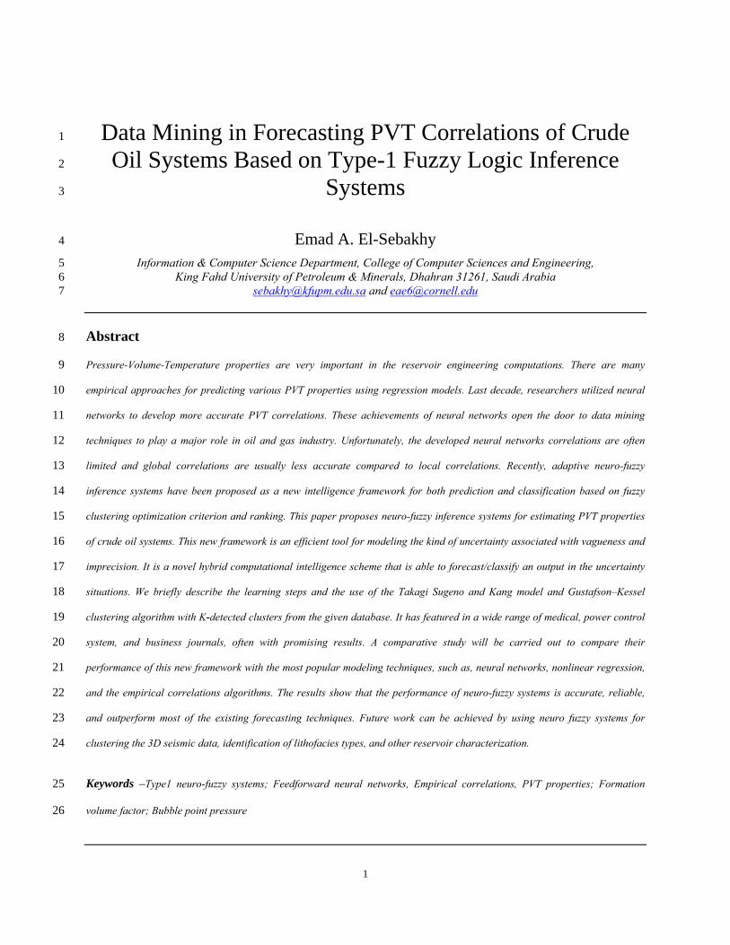
As it is shown in Figures 9 through 10, four scatter plots are drawn for the used three distinct databases. These

graphs show the measurements of both absolute percent relative error (EA) and correlation coefficient (R2) for type1

fuzzy logic inference systems scheme, feedforward neural networks (the used computational intelligence schemes)

and three empirical correlations. Each modeling scheme is represented by a symbol; the good forecasting scheme

should have the highest correlation and lowest absolute percent relative error.

20

Table 1 Testing results (Al-Marhoun (1988), El-Sebakhy et al. (2007), and Osman et al. (2001) data): Statistical quality measures when estimate Bo.

Correlation Er EA Emin Emax SD R2 Standing (1947) -0.170 2.724 0.008 20.180 2.5823 0.974

Glaso (1980) 1.8186 3.374 0.003 17.776 2.673 0.972 Al-Marhoun (1992) -0.115 2.205 0.003 13.179 1.2842 0.981

ANN System 0.3024 1.789 0.008 11.775 0.89835 0.988 Type1 Fuzzy Sys. 0.1501 1.322 0.002 7.4513 0.7876 0.997

Table 2 Testing results (Al-Marhoun (1988), El-Sebakhy et al. (2007), and Osman et al. (2001) data): Statistical quality measures when estimate Pb.

Correlation Er EA Emin Emax SD R2 Standing (1947) 67.60 67.73 0.1620 102.08 25.159 0.867

Glaso (1980) -1.616 18.52 0.1056 138.96 25.171 0.945 Al-Marhoun (1992) 8.008 20.01 0.0254 109.12 12.839 0.906

ANN System 8.129 21.02 0.0182 145.29 14.871 0.943 Type1 Fuzzy Sys. 7.432 14.22 0.0093 101.23 11.337 0.952

1 2

3

4

5

6

7

8

By looking at these scatter plots; we observed for example, in estimating Bo based on the data set used in

Abdulraheem et al. (2007), the symbol corresponding to Type1 fuzzy has the smallest absolute percent relative

error, EA = 1.3218%, the largest correlation coefficient, R2 = 0.9970, and the smallest standard deviation, SD =

0.7876, while neural network is below type1 fuzzy logic inference systems scheme with EA = 1.7886%, R2 =

0.9878, and SD = 0.89835. The other empirical correlations indicates higher error values with lower correlation

coefficients, for instance, Al-Marhoun (1992) has EA = 2.2053%, R2 = 0.9806, and SD = 1.2842; Standing has EA =

2.7238%, R2 = 0.9742, and SD = 2.673; and Glaso Correlation with EA = 3.3743%, R2 = 0.9715, and SD = 2.583.

Table 3 Testing results (Al-Marhoun et al. (2002) and Osman et al. (2002 and 2005) dataset): Statistical quality measures when estimate Bo.

Correlation Er EA Emin Emax SD R2 Standing (1947) -1.054 1.6833 0.066 7.7997 2.1021 0.9947

Glaso (1980) 0.4538 1.7865 0.0062 7.3839 2.1662 0.9920 Al-Marhoun (1992) -0.392 0.8451 0.0003 3.5546 1.1029 0.9972

ANN System 0.217 0.5116 0.0061 2.6001 0.6626 0.9977 Type1 Fuzzy Sys. 0.016 0.3247 0.0011 2.3365 0.3856 0.997

21

Table 4 Testing results (Al-Marhoun et al. (2002) and Osman et al. (2002 and 2005) dataset): Statistical quality measures when estimate Pb.

Correlation Er EA Emin Emax SD R2 Standing (1947) -8.441 10.4562 0.2733 47.0213 11.841 0.8974

Glaso (1980) -18.48 20.7569 2.0345 63.7634 16.160 0.9837 Al-Marhoun (1992) 0.941 8.1028 0.0935 38.085 11.41 0.9905

ANN System -0.222 5.8915 0.2037 38.1225 8.678 0.9930 Type1 Fuzzy Sys. -0.456 3.186 0.0012 24.347 4.82 0.995

Table 5 Testing results (Goda et al. (2003) and Osman et al. (2001) dataset): Statistical quality measures when estimate Bo.

Correlation Er EA Emin Emax SD R2 Standing (1947) -2.628 2.7202 0.0167 13.2922 5.7655 0.9953 Glaso (1980) -0.5529 0.9821 0.0086 6.5123 5.2274 0.9959

Al-Marhoun (1992) -0.4514 2.0084 0.0322 11.0755 5.0028 0.9935 ANN System 0.3251 1.4592 0.0083 5.3495 4.7402 0.9968

Type1 Fuzzy Sys. 0.0621 0.2456 0.0043 2.4013 4.5873 0.9971

Table 6 Testing results (Goda et al. (2003) and Osman et al. (2001) dataset): Statistical quality measures when estimate Pb.

Correlation Er EA Emin Emax SD R2 Standing (1947) 12.811 24.684 0.62334 59.038 13.696 0.8657

Glaso (1980) -18.887 26.551 0.28067 98.78 25.27 0.9675 Al-Marhoun (1992) 5.1023 8.9416 0.13115 87.989 25.015 0.9701

ANN System 4.9205 6.7495 0.16115 65.3839 22.73 0.9765 Type1 Fuzzy System 3.2218 4.0651 0.1178 52. 1921 15.821 0.9781

Similarly, for the bubble point pressure, Pb based on the used data sets used in Al-Marhoun et al. (2002), El-

Sebakhy et al. (2007), Goda et al. (2003), and Osman et al. (2001 and 2002), we observed that the symbol

corresponding to Type1 Fuzzy scheme has the smallest absolute percent relative error, EA = 14.224%, the largest

correlation coefficient, R2 = 0.9520, and the smallest standard deviation, SD = 11.337, while neural network is

below Type1 Fuzzy with EA = 21.017%, R2 = 0.943, and SD = 14.871. The other correlations indicates higher

error values with lower correlation coefficients, for instance, Al-Marhoun (1992) has EA = 20.011%, R2 = 0.906,

and SD = 12.839; Standing has EA = 67.73%, R2 = 0.867, and SD = 25.171; and Glaso empirical correlation with

EA = 18.523%, R2 = 0.945, and SD = 25.159. Overall computations, we observed that the new intelligence system

framework has a reasonable value of the relative errors, Er, especially, by looking at Tables 5 and 6, the Type1

neuro-fuzzy system has the smallest Er values compared to the other published techniques. This indicator can be

used as a very good indicator to say that the performance of the new framework is the one with the least bias.

1

2

3

4

5

6

7

8

9

10

11

22

Figure 9: Average Absolute relative errors and Correlation coefficients when we run the provided data sets under type1 fuzzy inference systems, neural network, and three empirical correlations for predicting Bob.

1

2

3

4

5

6

7

The same implementations processes may be repeated for the other statistical quality measures, but for the sake

of simplicity, we did not include it in this context. Finally, we conclude that developed type1 fuzzy inference

systems modeling scheme has better and reliable performance compared to the most published modeling schemes

and empirical correlations. The bottom line is that, the developed type1 fuzzy inference systems modeling scheme

outperforms both the standard feedforward neural networks and the most common published empirical correlations

in predicting both Pb and Bo using the four input variables: solution gas-oil ratio, reservoir temperature, oil gravity,

and gas relative density.

23

Figure 10: Average Absolute relative errors and Correlation coefficients when we run the provided data sets

under type1 fuzzy inference systems, neural network, and three empirical correlations for predicting Pb.

6. Conclusion and Recommendation 1

2

3

4

5

6

7

8

9

In this study, three distinct published data sets were used in investigating the capability of the type1 fuzzy

inference systems scheme as a new framework for predicting the PVT properties of oil crude systems. Based on the

obtained results and comparative studies, the conclusions and recommendations can be drawn as follows:

A new computational intelligence modeling scheme based on the type1 fuzzy inference systems scheme to

predict both bubble point pressure and oil formation volume factor using the four input variables: solution gas-oil

ratio, reservoir temperature, oil gravity, and gas relative density. As it is shown in the petroleum engineering

communities, these two predicted properties were considered the most important PVT properties of oil crude

systems.

24

- The developed type1 fuzzy inference systems scheme outperforms both the standard feedforward neural 1

networks and the most common published empirical correlations. Thus, the developed type1 fuzzy logic 2

inference systems scheme has better, efficient, and reliable performance compared to the most published 3

correlations. 4

- The developed type1 fuzzy inference systems scheme showed a high accuracy in predicting the Bo values with a 5

stable performance, and achieved the lowest absolute percent relative error, lowest minimum error, lowest 6

maximum error, lowest RMSE and the highest R2 among other correlations for the used three distinct data sets. 7

- The developed type1 fuzzy inference intelligence framework performance showed the smallest standard 8

deviation values all over the entire datasets utilized in the manipulation process, which indicates that the new 9

framework is more stable and robust than the most published techniques. Since the initial topology of the new

framework take into consideration the entire input domain in both GK clustering and membership functions.

Therefore, there is no any risk of over-fitting and complexity problems and then there is no lack of robustness

in prediction.

10

11

12

13

15

16

18

19

20

21

22

23

24

25

26

- The new intelligence system framework has a reasonable value of the relative errors, Er, especially, by looking 14

at Tables 5 and 6, the Type1 neuro-fuzzy system has the smallest Er values compared to the other published

techniques. This indicator indicates that the performance of the new framework is the one with the least bias.

- The type1 fuzzy inference modeling scheme is flexible, reliable, and shows a bright future in implementing it 17

for the oil and gas industry, especially permeability and porosity prediction, history matching, rock mechanics

properties, flow regimes and liquid-holdup multiphase follow, 3D seismic data, and faceis classification.

NOMENCLATURE

Bob = OFVF at the bubble- point pressure, RB/STB

Rs = oil solution gas oil ratio, SCF/STB

T = reservoir temperature, degrees Fahrenheit

γo = oil relative density (water=1.0)

γg = gas relative density (air=1.0)

Er = average percent relative error

25

Ei = percent relative error 1

2

3

4

5

6

7

8

9

10

11

12

13

14

15

16

17

18

19

20

21

22

23

Ea = average absolute percent relative error

Emax = Maximum absolute percent relative error

Emin = Minimum absolute percent relative error

RMS = Root Mean Square error

Acknowledgement

The author wishes to thank King Fahd University of Petroleum and Minerals, Mansoura University, and Cornell

University for the facilities utilized to perform the present work and for their support.

References

Abdulraheem A., El-Sebakhy E. A., Ahmad M., Vantala A., Korvin G., and Raharja I. P., 2007. “The Capability of

Neuro-Fuzzy` Systems in Predicting Permeability and Porosity from Well-Log”. SPE105350, the SPE 15th

Middle East Oil Show held in Bahrain, 11–14 March.

Ali J. K., 1994. “Neural Networks: A New Tool for the Petroleum Industry”. SPE 27561 presented at the 1994

European Petroleum Computer Conference, Aberdeen, U.K., March 15-17.

Al-Marhoun M., “PVT Correlations for Middle East Crude Oils,” Journal of Petroleum Technology, pp 650-666,

1988.

Al-Marhoun M. A., 1992. “New Correlation for formation Volume Factor of oil and gas Mixtures,” JCPT , March

22.

Al-Marhoun M.A. and Osman E. A., 2002. “Using Artificial Neural Networks to Develop New PVT Correlations

for Saudi Crude Oils”. SPE 78592, presented at the 10th Abu Dhabi International Petroleum Exhibition and

Conference (ADIPEC), Abu Dhabi, UAE, October 8-11.

Al-Shammasi A. A., 1997. “Bubble Point Pressure and Oil Formation Volume Factor Correlations”. SPE 53185

presented at the 1997 SPE Middle East Oil Show and Conference, Bahrain, March 15–18.

26

1

2

3

4

5

6

7

8

9

10

11

12

13

14

15

16

17

18

19

20

21

22

23

24

25

26

27

Al-Shammasi A. A., 2001. “A Review of Bubble point Pressure and Oil Formation Volume Factor Correlations”.

SPE Reservoir Evaluation & Engineering, 146-160. This paper (SPE 71302) was revised for publication of

paper SPE 53185.

Amabeoku M., Lin O., Khalifa C., Cole A. A., Dahan J., Jarlow M. J., and Ajufo A., (2005). “Use of Fuzzy-Logic

Permeability Models to Facilitate 3D Geocellular Modeling and Reservoir Simulation: Impact on Business”.

Presented at the International Petroleum Technology Conf., 21-23 November, Doha, Qatar.

Bezdek, J., Keller, J., Krisnapuram, R., Pal, N.R., (2005). Fuzzy Models and Algorithms for Pattern Recognition

and Image Processing. Boston Kluwer Academy Publishers.

Cuddy S. J., (1998). “Litho-Facies and Permeability Prediction from Electrical Logs using Fuzzy Logic”.

SPE49470 Presented at 8th Abu Dhabi International Petroleum Exhibition and Conference, (1998).

Duda R. O., Hart P. E., and Stock D. G., (2001). , “Pattern Classification, 2nd E, John Wiley and Sons, New York.

Dumitrescu, D., Lazzerini, B., Jain, L., (2000). Fuzzy Sets and Their Applications to Clustering and Training,

(2000) , Florida CRC Press.

El-Sebakhy E. A., El-Shaltami T. R., Al-Bukhitan S. Y., Shabaan Y. M., Raharja I. P., and Khaeruzzaman Y.,

(2007). “Support Vector Machines Framework for Predicting the PVT Properties of Crude Oil Systems”, the

SPE 15th Middle East Oil Show held in Bahrain, 11–14 March 2007. SPE105698.

El-Sebakhy E. A., Shabaan Y. M., Raharja I. P., and Khaeruzzaman Y., (2007).“Neuro-Fuzzy Inference Systems in

Identifying Flow-Regimes and Liquid-Holdup in Horizontal Multiphase Flow”. ICMSAO’07. Second Int.

Conf. on Modeling, Simulation and Applied Optimization. March 24–27. The PI, Abu Dhabi, UAE.

Elsharkawy A. M., (1998). “Modeling the Properties of Crude Oil and Gas Systems Using RBF Network”. SPE

49961 presented at the SPE Asia Pacific Oil and Gas Conference, Perth, Australia, October 12-14.

Glazo O., 1980. “Generalized Pressure-Volume Temperature Correlations,” JPT May, 785.

Goda H. M., Shokir E. M., Fattah K. A., and Sayyouh M. H., 2003. ” Prediction of the PVT Data Using Neural

Network Computing Theory”. SPE 85650, the 27th Annual SPE International Conference and Exhibition,

Abuja, Nigeria, August 4-6.

Gharbi R. B. and Elsharkawy A. M., 1997. “Neural-Network Model for Estimating the PVT Properties of Middle

East Crude Oils”. SPE 37695 presented at the 1997 SPE Middle East Oil Conference, Bahrain, 15–18.

27

1

2

3

4

5

6

7

8

9

10

11

12

13

14

15

16

17

18

19

20

21

22

23

24

25

26

Gharbi R. B. and Elsharkawy A.M., (1997). “Universal Neural-Network Model for Estimating the PVT Properties

of Crude Oils,” SPE 38099 presented at the 1997 SPE Asia Pacific Oil & Gas Conference, Kuala Lumpur,

Malaysia, April 14-16.

Hambalek N. and Reinaldo G., (2003). “Fuzzy logic applied to lithofacies and permeability forecasting”. SPE

(81078) presented at SPE Latin America and Caribbean Petroleum Engineering Conf., Spain, Trinidad, West

Indies.

Jong-Se L. and Kim J., (2004) ”Reservoir Porosity and Permeability Estimation from Well Logs Using Fuzzy

Logic and Neural Networks”. SPE 88476. Presented at SPE Asia Pacific Oil and Gas Conference and

Exhibition. Perth, Australia.

Kumoluyi A. O. and Daltaban T. S., 1994. “High Order Neural Network in Petroleum Engineering”. SPE 27905

presented at the 1994 SPE Western Regional Meeting, Longbeach, California, USA, March 23-25.

LeCun Y., Botou L., Jackel L., Drucker H., Cortes C., Denker J., Guyon I., Muller U., Sackinger E., Simard P., and

Vapnik V., 1995. “Learning algorithms for classification: A comparison on handwritten digit recognition,”

Neural Netw., pp. 261–276.

Liu C., Nakashima K., Sako H., and Fujisawa H., 2003. “Handwritten digit recognition: Bench-marking of state-of-

the-art techniques,” Pattern Recognition, vol. 36, pp. 2271–2285.

McCain W. D. Jr., Soto R. B., Valko, P. P., and Blasingame T. A., 1998. “Correlation Of Bubble point Pressures

For Reservoir Oils - A Comparative Study”. SPE 51086 presented at the 1998 SPE Eastern Regional

Conference and Exhibition held in Pittsburgh, PA, 9–11.

Mohaghegh S. and Ameri S., 1994. "An Artificial Neural Network As A Valuable Tool for Petroleum Engineers".

SPE 29220, unsolicited paper for Society of Petroleum Engineers.

Mohaghegh S., 1995. “Neural Networks: What it Can do for Petroleum Engineers," JPT, 42.

Mohaghegh S., 2000. "Virtual Intelligence Applications in Petroleum Engineering: Part 1 - Artificial Neural

Networks”. JPT, September.

Osman E. A., Abdel-Wahhab O. A., and Al-Marhoun M. A., 2001. “Prediction of Oil Properties Using Neural

Networks,” Paper SPE 68233.

28

29

1

2

3

4

5

6

7

8

9

10

11

Osman E. A. and Abdel-Aal R., 2002. "Abductive Netwoks: A New Modeling Tool for the Oil and Gas Industry".

SPE 77882, Asia Pacific Oil and Gas Conference and Exhibition Melbourne, Australia, 8–10 October.

Osman E. and Al-Marhoun M., 2005. “Artificial Neural Networks Models for Predicting PVT Properties of Oil

Field Brines". SPE 93765, 14th SPE Middle East Oil & Gas Show and Conference in Bahrain, March.

Standing M. B., 1974. “A Pressure Volume Temperature (PVT) Correlation for Mixtures of California Oils and

Gases,” Drill&Prod. Pract., API, pp 275-87.

Taghavi, A. A., 2005. “Improved Permeability Estimation through use of Fuzzy Logic in a Carbonate Reservoir

from Southwest Iran”. Presented at SPE Middle East Oil and Gas Show and Conf., Mar 12 - 15, Bahrain.

Varotsis N., Gaganis V., Nighswander J., and Guieze P., 1999. “A Novel Non-Iterative Method for the Prediction of

the PVT Behavior of Reservoir Fluids”. SPE 56745 presented at the SPE Annual Technical Conference and

Exhibition, Houston, Texas, October 3–6.