Data J I Social - Copernicus.org

ESSDD5, 1107–1157, 2012

The global carbonbudget 1959–2011

C. Le Quere et al.

Title Page

Abstract Instruments

Data Provenance & Structure

Tables Figures

J I

J I

Back Close

Full Screen / Esc

Printer-friendly Version

Interactive Discussion

Discussion

Paper

|D

iscussionP

aper|

Discussion

Paper

|D

iscussionP

aper|

Earth Syst. Sci. Data Discuss., 5, 1107–1157, 2012www.earth-syst-sci-data-discuss.net/5/1107/2012/doi:10.5194/essdd-5-1107-2012© Author(s) 2012. CC Attribution 3.0 License.

History of Geo- and Space

SciencesOpen

Acc

ess

Advances in Science & ResearchOpen Access Proceedings

Ope

n A

cces

s Earth System

Science

Data Ope

n A

cces

s Earth System

Science

Data

Discu

ssions

Drinking Water Engineering and Science

Open Access

Drinking Water Engineering and Science

DiscussionsOpe

n Acc

ess

Social

Geography

Open

Acc

ess

Discu

ssions

Social

Geography

Open

Acc

ess

CMYK RGB

This discussion paper is/has been under review for the journal Earth System ScienceData (ESSD). Please refer to the corresponding final paper in ESSD if available.

The global carbon budget 1959–2011

C. Le Quere1, R. J. Andres2, T. Boden2, T. Conway3, R. A. Houghton4,J. I. House5, G. Marland6, G. P. Peters7, G. van der Werf8, A. Ahlstrom9,R. M. Andrew7, L. Bopp10, J. G. Canadell11, P. Ciais10, S. C. Doney12, C. Enright1,P. Friedlingstein13, C. Huntingford14, A. K. Jain15, C. Jourdain1,*, E. Kato16,R. F. Keeling17, K. Klein Goldewijk25, S. Levis18, P. Levy14, M. Lomas19,B. Poulter10, M. R. Raupach11, J. Schwinger20, S. Sitch21, B. D. Stocker22,N. Viovy10, S. Zaehle23, and N. Zeng24

1Tyndall Centre for Climate Change Research, University of East Anglia, Norwich ResearchPark, Norwich, NR4 7TJ, UK2Carbon Dioxide Information Analysis Center (CDIAC), Oak Ridge National Laboratory,Oak Ridge, Tennessee, USA3National Oceanic & Atmosphere Administration, Earth System Research Laboratory(NOAA/ESRL), Boulder, Colorado 80305, USA4Woods Hole Research Centre (WHRC), Falmouth, Massachusetts 02540, USA5Cabot Institute, Dept of Geography, University of Bristol, UK6Research Institute for Environment, Energy, and Economics, Appalachian State University,Boone, North Carolina 28608, USA7Center for International Climate and Environmental Research – Oslo (CICERO), Norway8Faculty of Earth and Life Sciences, VU University Amsterdam, The Netherlands9Department of Physical Geography and Ecosystem Science, Lund University, Sweden

1107

http://www.earth-syst-sci-data-discuss.net

http://www.earth-syst-sci-data-discuss.net/5/1107/2012/essdd-5-1107-2012-print.pdf

http://www.earth-syst-sci-data-discuss.net/5/1107/2012/essdd-5-1107-2012-discussion.html

http://creativecommons.org/licenses/by/3.0/

ESSDD5, 1107–1157, 2012


C. Le Quere et al.

Title Page



Tables Figures

J I

J I

Back Close

Full Screen / Esc



Discussion

Paper

|D

iscussionP

aper|

Discussion

Paper

|D

iscussionP

aper|

10Laboratoire des Sciences du Climat et de l’Environnement, CEA-CNRS-UVSQ,CE Orme des Merisiers, 91191 Gif sur Yvette Cedex, France11Global Carbon Project, CSIRO Marine and Atmospheric Research, Canberra, Australia12Woods Hole Oceanographic Institution (WHOI), Woods Hole, MA 02543, USA13College of Engineering, Mathematics and Physical Sciences, University of Exeter, Exeter,EX4 4QF, UK14Centre for Ecology and Hydrology (CEH), Wallingford, OX10 8BB, UK15Department of Atmospheric Sciences, University of Illinois, USA16Center for Global Environmental Research (CGER), National Institute for EnvironmentalStudies (NIES), Japan17University of California, San Diego, Scripps Institution of Oceanography, La Jolla,California 92093-0244, USA18National Center for Atmospheric Research (NCAR), Boulder, Colorado, USA19Centre for Terrestrial Carbon Dynamics (CTCD), Sheffield University, UK20Geophysical Institute, University of Bergen & Bjerknes Centre for Climate Research,Bergen, Norway21College of Life and Environmental Sciences, University of Exeter, Exeter, EX4 4RJ, UK22Physics Institute, and Oeschger Centre for Climate Change Research, University of Bern,Switzerland23Max-Planck-Institut fur Biogeochemie, P.O. Box 600164, Hans-Knoll-Str. 10, 07745 Jena,Germany24Department of Atmospheric and Oceanic Science, University of Maryland, USA25PBL Netherlands Environmental Assessment Agency, The Hague/Bilthoven,The Netherlands*now at: Food and Agriculture Organization of the United Nations (FAO), Rome, Italy

Received: 20 November 2012 – Accepted: 21 November 2012 – Published: 2 December 2012

Correspondence to: C. Le Quere ([email protected])

Published by Copernicus Publications.

1108





ESSDD5, 1107–1157, 2012


C. Le Quere et al.

Title Page



Tables Figures

J I

J I

Back Close

Full Screen / Esc



Discussion

Paper

|D

iscussionP

aper|

Discussion

Paper

|D

iscussionP

aper|

Abstract

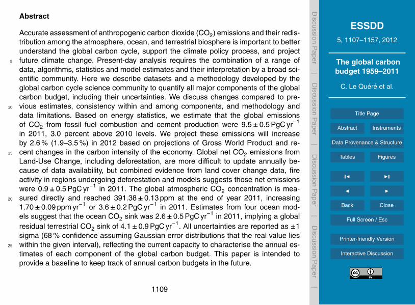
Accurate assessment of anthropogenic carbon dioxide (CO2) emissions and their redis-tribution among the atmosphere, ocean, and terrestrial biosphere is important to betterunderstand the global carbon cycle, support the climate policy process, and projectfuture climate change. Present-day analysis requires the combination of a range of5

data, algorithms, statistics and model estimates and their interpretation by a broad sci-entific community. Here we describe datasets and a methodology developed by theglobal carbon cycle science community to quantify all major components of the globalcarbon budget, including their uncertainties. We discuss changes compared to pre-vious estimates, consistency within and among components, and methodology and10

data limitations. Based on energy statistics, we estimate that the global emissionsof CO2 from fossil fuel combustion and cement production were 9.5±0.5 PgC yr−1

in 2011, 3.0 percent above 2010 levels. We project these emissions will increaseby 2.6 % (1.9–3.5 %) in 2012 based on projections of Gross World Product and re-cent changes in the carbon intensity of the economy. Global net CO2 emissions from15

Land-Use Change, including deforestation, are more difficult to update annually be-cause of data availability, but combined evidence from land cover change data, fireactivity in regions undergoing deforestation and models suggests those net emissionswere 0.9±0.5 PgC yr−1 in 2011. The global atmospheric CO2 concentration is mea-sured directly and reached 391.38±0.13 ppm at the end of year 2011, increasing20

1.70±0.09 ppm yr−1 or 3.6±0.2 PgC yr−1 in 2011. Estimates from four ocean mod-els suggest that the ocean CO2 sink was 2.6±0.5 PgC yr−1 in 2011, implying a globalresidual terrestrial CO2 sink of 4.1±0.9 PgC yr−1. All uncertainties are reported as ±1sigma (68 % confidence assuming Gaussian error distributions that the real value lieswithin the given interval), reflecting the current capacity to characterise the annual es-25

timates of each component of the global carbon budget. This paper is intended toprovide a baseline to keep track of annual carbon budgets in the future.

1109





ESSDD5, 1107–1157, 2012


C. Le Quere et al.

Title Page



Tables Figures

J I

J I

Back Close

Full Screen / Esc



Discussion

Paper

|D

iscussionP

aper|

Discussion

Paper

|D

iscussionP

aper|

All carbon data presented here can be downloaded from the Carbon Dioxide Infor-mation Analysis Center (doi:10.3334/CDIAC/GCP V2012).

1 Introduction

The concentration of carbon dioxide (CO2) in the atmosphere has increased from ap-proximately 278 parts per million (ppm) in 1750, the beginning of the Industrial Era, to5

391.4 at the end of 2011 (Conway and Tans, 2012). This increase was caused initiallymainly by the anthropogenic release of carbon to the atmosphere from deforestationand other land-use change activities. Emissions from fossil fuel combustion startedbefore the Industrial Revolution and became the dominant source of anthropogenicemissions to the atmosphere from around 1920 until present. Anthropogenic emis-10

sions occur on top of an active natural carbon cycle that circulates carbon between theatmosphere, ocean, and terrestrial biosphere reservoirs on time scales from days tomany millennia, while geologic reservoirs have even longer timescales (Archer et al.,2009).

The “global carbon budget” presented here refers to the direct and indirect anthro-15

pogenic perturbation of CO2 in the atmosphere. It quantifies the input of CO2 to theatmosphere by emissions from human activities, the growth of CO2 in the atmosphere,and the resulting changes in land and ocean carbon fluxes directly in response to in-creasing atmospheric CO2 levels and indirectly in response to climate and other anthro-pogenic changes. An understanding of this perturbation budget over time and the un-20

derlying variability and trends of the natural carbon cycle are necessary to understandand quantify climate-carbon feedbacks. This also allows potentially earlier detection ofany approaching discontinuities or tipping points of the carbon cycle in response toanthropogenic changes (Falkowski et al., 2000).

The components of the CO2 budget that are reported in this paper include separate25

estimates for (1) the CO2 emissions from fossil fuel combustion and cement produc-tion (EFF), (2) the CO2 emissions resulting from deliberate human activities on land,

1110





http://dx.doi.org/10.3334/CDIAC/GCP_V2012

ESSDD5, 1107–1157, 2012


C. Le Quere et al.

Title Page



Tables Figures

J I

J I

Back Close

Full Screen / Esc



Discussion

Paper

|D

iscussionP

aper|

Discussion

Paper

|D

iscussionP

aper|

including land use, land-use change and forestry (shortened to LUC hereafter; ELUC),(3) the growth rate of CO2 in the atmosphere (GATM), and (4) the uptake of CO2 by the“CO2 sinks” in the ocean (SOCEAN) and on land (SLAND). The CO2 sinks as defined hereinclude the response of the land and oceans to elevated CO2 and changes in climateand other environmental conditions. The emissions and their partitioning among the5

atmosphere, ocean and land are in balance:

EFF +ELUC = GATM +SOCEAN +SLAND (1)

Equation (1) subsumes, and partly omits, two kinds of processes. The first is the net in-put of CO2 to the atmosphere from the chemical oxidation of reactive carbon-containinggases, primarily methane (CH4), carbon monoxide (CO), and volatile organic com-10

pounds such as terpene and isoprene, which we quantify here for the first time. Thesecond is the anthropogenic perturbations to inland freshwaters, estuaries, and coastalareas carbon cycling, that modify both lateral fluxes transported from land ecosystemsto the open ocean, and “vertical” CO2 fluxes of rivers and estuaries outgassing, andthe air-sea CO2 net exchange of coastal areas (Battin et al., 2008; Aufdenkampe et15

al., 2011). These flows are omitted in absence of details on the natural versus an-thropogenic terms of these loops of the carbon cycle. The inclusion of these fluxes ofanthropogenic CO2 would affect the estimates of SLAND and perhaps SOCEAN in Eq. (1),but not GATM.

The global carbon budget has been assessed by the Intergovernmental Panel on20

Climate Change (IPCC) in all Assessment reports (Watson et al., 1990; Schimel et al.,1995; Prentice et al., 2001; Denman et al., 2007), and by others (Conway and Tans,2012). These included budget estimates for the decades of the 1980s, 1990s and, mostrecently, the period 2000–2005. The IPCC methodology has been adapted and used bythe Global Carbon Project (GCP, www.globalcarbonproject.org), who have coordinated25

a cooperative community effort for the annual publication of global CO2 budgets foryear 2005 (Raupach et al., 2007; including fossil emissions only), year 2006 (Canadellet al., 2007), year 2007 (published online), year 2008 (Le Quere et al., 2009), year 2009

1111





www.globalcarbonproject.org

ESSDD5, 1107–1157, 2012


C. Le Quere et al.

Title Page



Tables Figures

J I

J I

Back Close

Full Screen / Esc



Discussion

Paper

|D

iscussionP

aper|

Discussion

Paper

|D

iscussionP

aper|

(Friedlingstein et al., 2010), and most recently, year 2010 (Peters et al., 2012b). Eachof these papers updated previous estimates with the latest available information forthe entire time series. From 2008, these publications projected fossil fuel emissions forone additional year using the projected World Gross Domestic Product and estimatedimprovements in the carbon intensity of the economy.5

We adopt a range of ±1 standard deviation (sigma) to report the uncertainties inour annual estimates, representing a likelihood of 68 % that the true value lies withinthe provided range, assuming that the errors have a Gaussian distribution. This choicereflects the difficulty of characterising the uncertainty in the CO2 fluxes between theatmosphere and the ocean and land reservoirs individually, as well as the difficulty to10

update the CO2 emissions from LUC, particularly on an annual basis. A 68 % likelihoodprovides an indication of our current capability to quantify each term and its uncer-tainty given the available information. For comparison, the Fourth Assessment Reportof the IPCC (AR4) generally reported 90 % uncertainty for large datasets whose un-certainty is well characterised, or for long time intervals less affected by year-to-year15

variability. This includes, for instance, attribution statements associated with recordedwarming levels since the pre-industrial period. The 90 % number corresponds to theIPCC language of “very likely” or “very high confidence represents at least a 9 out of10 chance”; our 68 % value is near the 66 % which the IPCC reports as only “likely”.The uncertainties reported here combine statistical analysis of the underlying data and20

expert judgement of the likelihood of results lying outside this range. The limitations ofcurrent information are discussed in the paper.

All units are presented in petagrammes of carbon (PgC, 1015 gC), which is the sameas gigatonnes of carbon (GtC). Units of gigatonnes of CO2 (or billion tonnes of CO2)used in policy circles are equal to 3.67 multiplied by the value in units of PgC.25

This paper provides a detailed description of the datasets and methodology usedto compute the global CO2 budget and associated uncertainties for the period 1959–2011. It presents the global CO2 budget estimates by decade since the 1960s, includ-ing the last decade (2002–2011), the results for the year 2011, and a projection of

1112





ESSDD5, 1107–1157, 2012


C. Le Quere et al.

Title Page



Tables Figures

J I

J I

Back Close

Full Screen / Esc



Discussion

Paper

|D

iscussionP

aper|

Discussion

Paper

|D

iscussionP

aper|

EFF for year 2012. It is intended that this paper will be updated every year using theformat of “living reviews”, to help keep track of new versions of the budget that re-sult from new data, revision of data, and changes in methodology. Additional materialsassociated with the release of each new version will be posted at the Global Car-bon Project (GCP) website (http://www.globalcarbonproject.org/carbonbudget). With5

this approach, we aim to provide transparency and traceability in reporting indicatorsand drivers of climate change.

2 Methods

The original data and measurements to complete the global carbon budget are gener-ated by multiple organizations and research groups around the world. The effort pre-10

sented here is thus mainly one of synthesis, where results from individual groups arecollated, analysed and evaluated for consistency. Descriptions of the measurements,models, and methodologies follow below and in depth descriptions of each componentare described elsewhere (e.g. Andres et al., 2012; Houghton et al., 2012).

2.1 CO2 emissions from fossil fuel combustion and cement production (EFF)15

2.1.1 Fossil fuel and cement emissions and their uncertainty

The calculation of global and national CO2 emissions from fossil fuel combustion, in-cluding gas flaring and cement production (EFF), relies primarily on energy data, specif-ically data on hydrocarbon fuels, collated and archived by several organisations (An-dres et al., 2012), including the Carbon Dioxide Information Analysis Center (CDIAC),20

the International Energy Agency (IEA), the United Nations (UN), and the United StatesDepartment of Energy (DoE) Energy Information Administration (EIA). We use theemissions estimated by the CDIAC (http://cdiac.ornl.gov) which are based primarilyon energy data provided by the UN Statistics Division (UN, 2012a, b) (Table 1), andare typically available 2–3 yr after the close of a given year. CDIAC also provides the25

1113





http://www.globalcarbonproject.org/carbonbudget

http://cdiac.ornl.gov

ESSDD5, 1107–1157, 2012


C. Le Quere et al.

Title Page



Tables Figures

J I

J I

Back Close

Full Screen / Esc



Discussion

Paper

|D

iscussionP

aper|

Discussion

Paper

|D

iscussionP

aper|

only dataset that extends back in time to 1751 with consistent and well-documentedemissions from all fossil fuels, cement production, and gas flaring for all countries (andtheir uncertainty); this makes the dataset a unique resource for research of the carboncycle during the fossil fuel era. For this paper, we use CDIAC emissions data up to pe-riod 1959–2009, and preliminary estimates based on the BP annual energy review for5

emissions in 2010 and 2011 (BP, 2012). BP’s sources for energy statistics overlap withthose of the UN data but are compiled more rapidly, using a smaller group of mostlydeveloped countries and assumptions for missing data. The preliminary estimates arereplaced by the more complete CDIAC data when available. Past experience showsthat projections based on the BP data provide reliable estimates for the two most re-10

cent years when full data are not yet available from the UN (see Sect. 3.2).Emissions from cement production are based on cement data from the US Geolog-

ical Survey (Van Oss, 2011) up to year 2009, and from preliminary data for 2010 and2011 (US Geological Survey, 2012). Emission estimates from gas flaring are calcu-lated in a similar manner as those from solid, liquid, and gaseous fuels, and rely on the15

UN Energy Statistics to supply the amount of flared fuel. For emission years 2010 and2011, flaring estimates are assumed constant from the emission year 2009 UN-baseddata. The basic data on gas flaring have large uncertainty. Fugitive emissions of CH4from the so-called upstream sector (coal mining, oil extraction, gas extraction and dis-tribution) are not included in the accounts of CO2 emissions except to the extent that20

they get captured in the UN energy data and counted as gas “flared or lost”. The UNdata are not able to distinguish between gas that is flared or vented.

When necessary, fuel masses/volumes are converted to fuel energy content usingcoefficients provided by the UN and then to CO2 emissions using conversion factorsthat take into account the relationship between carbon content and heat content of25

the different fuel types (coal, oil, gas, gas flaring) and the combustion efficiency (toaccount, for example, for soot left in the combustor or fuel otherwise lost or dischargedwithout oxidation). In general, CO2 emissions for equivalent energy consumptions areabout 30 % higher for coal compared to oil, and 70 % higher for coal compared to gas

1114





ESSDD5, 1107–1157, 2012


C. Le Quere et al.

Title Page



Tables Figures

J I

J I

Back Close

Full Screen / Esc



Discussion

Paper

|D

iscussionP

aper|

Discussion

Paper

|D

iscussionP

aper|

(Marland et al., 2007). These calculations are based on the mass flows of carbon andassume that the carbon discharged as CO or CH4 will soon be oxidized to CO2 in theatmosphere and hence counts the carbon mass with CO2 emissions.

Emissions are estimated for 1959–2011 for 129 countries and regions. The disag-gregation of regions (e.g. the former Soviet Union prior to 1992) is based on the shares5

of emissions in the first year after the countries are disaggregated.Estimates of CO2 emissions show that the global total of emissions is not equal to

the sum of emissions from all countries. This is largely attributable to combustion offuels used in international shipping and aviation, where the emissions are included inthe global totals but are not attributed to individual countries. In practice, the emissions10

from international bunker fuels are calculated based on where the fuels were loaded,but they are not included with national emissions estimates. Smaller differences alsooccur because globally the sum of imports in all countries is not equivalent to the sumof exports, because of differing treatment of oxidation of non-fuel uses of hydrocarbons(e.g. as solvents, lubricants, feedstocks, etc.).15

The uncertainty of the annual fossil fuel and cement emissions for the globe hasbeen estimated at ±5 % (scaled down from the published 10 % at ±2 sigma to the useof ±1 sigma bounds reported here) (Andres et al., 2012). This includes an assessmentof the amounts of fuel consumed, the carbon contents of fuels, and the combustionefficiency. While in the budget we consider a fixed uncertainty of 5 % for all years, in20

reality the uncertainty, as a percentage of the emissions, is growing with time becauseof the larger share of global emissions from non-Annex B countries with weaker statis-tical systems (Marland et al., 2009). For example, the uncertainty in Chinese emissionsestimates has been estimated at around ±10 % (±1 sigma; Gregg et al., 2008). Gener-ally, emissions from mature economies with good statistical bases have an uncertainty25

of only a few percent (Marland, 2008).

1115





ESSDD5, 1107–1157, 2012


C. Le Quere et al.

Title Page



Tables Figures

J I

J I

Back Close

Full Screen / Esc



Discussion

Paper

|D

iscussionP

aper|

Discussion

Paper

|D

iscussionP

aper|

2.1.2 Emissions embodied in goods and services

National emissions inventories take a territorial (production) perspective by “in-clude[ing] all greenhouse gas emissions and removals taking place within national(including administered) territories and offshore areas over which the country has juris-diction” (from the Revised 1996 IPCC Guidelines for National Greenhouse Gas Inven-5

tories). That is, emissions are allocated to the country where and when the emissionsactually occur. The emission inventory of an individual country does not include theemissions from the production of goods and services produced in other countries (e.g.food and clothes) that are used for national consumption. The difference between thestandard territorial emission inventories and consumption-based emission inventories10

is the net transfer (exports minus imports) of emissions from the production of interna-tionally traded goods and services. Complementary emission inventories that allocatedemissions to the final consumption of goods and services (e.g. Davies et al., 2011) pro-vide additional information that can be used to understand emission drivers, quantifyemission leakages between countries, and potentially design more effective and effi-15

cient climate policy.We estimate consumption-based emissions by enumerating the global supply chain

using a global model of the economic relationships between sectors in every coun-try (Peters et al., 2011a). Due to availability of the input data, detailed estimates aremade for the years 1997, 2001, 2004, and 2007 (Peters et al., 2011a) using economic20

and trade data from the Global Trade and Analysis Project (GTAP; Narayanan et al.,2012). The results cover 57 sectors and up to 129 countries and regions. The resultsare extended into an annual time-series from 1990 to the latest year of the fossil-fuelemissions or GDP data (2010 in this budget), using GDP data by expenditure (fromthe UN Main Aggregates database, UN, 2012c) and time series of trade data from25

GTAP (Peters et al., 2012b). We do not provide an uncertainty estimate for these emis-sions, but based on model comparisons and sensitivity analysis, they are unlikely tobe significantly larger than for the territorial emission estimates (Peters et al., 2011b).

1116





ESSDD5, 1107–1157, 2012


C. Le Quere et al.

Title Page



Tables Figures

J I

J I

Back Close

Full Screen / Esc



Discussion

Paper

|D

iscussionP

aper|

Discussion

Paper

|D

iscussionP

aper|

Uncertainty is expected to increase for more detailed results (Peters et al., 2011b) (e.g.the results for Annex B will be more accurate than the sector results for an individualcountry).

It is important to note that the consumption-based emissions defined here considerdirectly the carbon embodied in traded goods and services, but not the trade in unox-5

idised fossil fuels (coal, oil, gas). In our consumption-based inventory, emissions fromtraded fossil fuels accrue to the country where the fuel is burned or consumed, not theexporting country from which it was extracted.

The consumption-based emission inventories in this carbon budget have several im-provements over previous years. The detailed estimates for 2004 and 2007 are based10

on an updated version of the GTAP database (Narayanan et al., 2012). We estimatethe sector level CO2 emissions using our own calculations based on the GTAP dataand methodology, but scale the national totals to match the CDIAC estimates fromthe carbon budget. We do not include international transportation in our estimates.The time-series of trade data provided by GTAP covers the period 1995–2009 and our15

methodology uses the trade shares of this dataset. For the period 1990–1994 we as-sume the trade shares of 1995, while in 2010 we assume the trade shares of 2008since 2009 was heavily affected by the global financial crisis. We identified errors in thetrade shares of Taiwan and Netherlands in 2008 and 2009, and for these two countries,the trade shares for 2008–2010 are based on the 2007 trade shares.20

This data does not contribute to the global average terms in Eq. (1), but are rele-vant to the anthropogenic carbon cycle as they reflect the movement of carbon acrossthe Earth’s surface in response to human needs (both physical and economic). Fur-thermore, if national and international climate policies continue to develop in an un-harmonised way, then the trends reflected in these data will need to be accommodated25

by those developing policies.

1117





ESSDD5, 1107–1157, 2012


C. Le Quere et al.

Title Page



Tables Figures

J I

J I

Back Close

Full Screen / Esc



Discussion

Paper

|D

iscussionP

aper|

Discussion

Paper

|D

iscussionP

aper|

2.1.3 Emissions projections for the current year

Energy statistics are normally available around June for the previous year. We use theclose relationship between the growth in world Gross Domestic Product (GDP) and thegrowth in global emissions (Raupach et al., 2007) to project emissions for the currentyear. This is based on the so-called Kaya (also called IPAT) identity, whereby EFF is5

decomposed by the product of GDP and the fossil fuel carbon intensity of the economy(IFF) as follows:

EFF = GDP · IFF (2)

taking a time derivative of this equation gives:

dEFF

dt=

d(GDP · IFF)

dt(3)10

and applying the rules of calculus, assuming that GDP and IFF are independent:

dEFF

dt=

dGDPdt

· IFF +GDP ·dIFF

dt(4)

finally, dividing Eq. (4) by Eq. (2) gives:

1EFF

dEFF

dt=

1GDP

dGDPdt

+1IFF

dIFFF

dt(5)

where the left hand term is the relative growth rate of EFF, and the right hand terms15

are the relative growth rates of GDP and IFF, respectively, which can simply be addedlinearly to give overall growth rate. The growth rates are reported in percent below bymultiplying each term by 100. Because preliminary estimates of annual change in GDPare made well before the end of a calendar year, making assumptions on the growthrate of IFF allows us to make projections of the annual change in CO2 emissions well20

before the end of a calendar year.1118





ESSDD5, 1107–1157, 2012


C. Le Quere et al.

Title Page



Tables Figures

J I

J I

Back Close

Full Screen / Esc



Discussion

Paper

|D

iscussionP

aper|

Discussion

Paper

|D

iscussionP

aper|

2.1.4 Growth rate in emissions

We report the annual growth rate in emissions for adjacent years in percent by calcu-lating the difference between the two years and then comparing to the emissions in thefirst year: [(EFF(t0 +1)−EFF(t0))/EFF(t0)] ·100. This is the simplest method to charac-terise a one-year growth compared to the previous year. This has strong links with the5

more general way in which society presents economic change in journalistic circles,most often a comparison of present-day economic activity compared to the previousyear.

The growth rate of EFF over time periods of greater than one year can be re-writtenusing its logarithm equivalent as follows:10

1EFF

dEFF

dt=

d(lnEFF)

dt(6)

Here we calculate growth rates in emissions for multi-year periods (e.g. a decade)by fitting a linear trend to ln (EFF) in Eq. (6), reported in percent per year. We fit thelogarithm of EFF rather than EFF directly because this method ensures that computedgrowth rates satisfy Eq. (6). This method differs from previous papers (Raupach et al.,15

2007; Canadell et al., 2007; Le Quere et al., 2009) who computed the fit to EFF anddivided by average EFF directly, but the difference is very small (<0.05 %) in the caseof EFF.

2.2 CO2 emissions from land-use, land-use change and forestry (ELUC)

Net LUC emissions reported in our annual budget (ELUC) include CO2 fluxes from af-20

forestation, deforestation, logging (forest degradation and harvest activity), shifting cul-tivation (cycle of cutting forest for agriculture then abandoning), regrowth of forests fol-lowing wood harvest or abandonment of agriculture, fire-based peatland emissions andother land management practices (Table 2). Our annual estimate combines informationfrom a bookkeeping model (Sect. 2.2.1) primarily based on forest area change and25

1119





ESSDD5, 1107–1157, 2012


C. Le Quere et al.

Title Page



Tables Figures

J I

J I

Back Close

Full Screen / Esc



Discussion

Paper

|D

iscussionP

aper|

Discussion

Paper

|D

iscussionP

aper|

biomass data from the Forest Resource Assessment (FRA) of the Food and AgricultureOrganisation (FAO) (Houghton, 2003) published at intervals of five years, with annualemissions estimated from satellite-based fire activity in deforested areas (Sect. 2.2.2;van der Werf et al., 2010). The bookkeeping model is used mainly to quantify the meanELUC over the time period of the available data, and the satellite-based method to dis-5

tribute these emissions annually. The satellite-based emissions are available from year1997 onwards only. We also use independent estimates from Dynamic Global Vegeta-tion Models (Sect. 2.2.3) to help quantifying the uncertainty in global ELUC.

2.2.1 Bookkeeping method

ELUC calculated using a bookkeeping method (Houghton, 2003) keeps track of the10

carbon stored in vegetation and soils before deforestation or other land-use change,and the changes in forest age classes, or cohorts, of disturbed lands after land-usechange. It tracks the CO2 emitted to the atmosphere over time due to decay of soil andvegetation carbon in different pools, including wood products pools after logging anddeforestation. It also tracks the regrowth of vegetation and build-up of soil carbon pools15

following land-use change. It considers transitions between forests, pastures and crop-land, shifting cultivation, degradation of forests where a fraction of the trees is removed,abandonment of agricultural land, and forest management such as logging and firemanagement. In addition to tracking logging debris on the forest floor, the bookkeepingmodel tracks the fate of carbon contained in harvested wood products that is eventually20

emitted back to the atmosphere as CO2, although a detailed treatment of the lifetime ineach product pool is not performed (Earles et al., 2012). Harvested wood products arepartitioned into three pools with different turnover times. All fuel-wood is assumed to beburned in the year of harvest (1.0 yr−1). Pulp and paper products are oxidized at a rateof 0.1 yr−1. Timber is assumed to be oxidized at a rate of 0.01 yr−1, and elemental car-25

bon decays at 0.001 yr−1. The general assumptions about partitioning wood productsamong these pools are based on national harvest data.

1120





ESSDD5, 1107–1157, 2012


C. Le Quere et al.

Title Page



Tables Figures

J I

J I

Back Close

Full Screen / Esc



Discussion

Paper

|D

iscussionP

aper|

Discussion

Paper

|D

iscussionP

aper|

The primary land-cover change and biomass data for the bookkeeping model anal-ysis is the FAO FRA 2010 (FAO, 2010) (Table 1), which is based on countries’ self-reporting of statistics on forest cover change and management partially combined withsatellite data in more recent assessments. Changes in land cover other than forest arebased on annual, national changes in cropland and pasture areas reported by the FAO5

Statistics Division (FAOSTAT, 2010). The LUC data set is non-spatial and aggregatedby regions. The carbon stocks on land (biomass and soils), and their response func-tions subsequent to LUC, are based on averages per land cover type, per biome andper region. Similar results were obtained using forest biomass carbon density basedon satellite data (Baccini et al., 2012). The bookkeeping model does not include land10

ecosystems’ transient response to changes in climate, atmospheric CO2 and other en-vironmental factors, but the growth/decay curves are based on contemporary data thatwill implicitly reflect the effects of CO2 and climate at that time.

2.2.2 Fire-based method

LUC CO2 emissions calculated from satellite-based fire activity in deforested areas15

(van der Werf et al., 2010) provide information that is complementary to the bookkeep-ing approach. Although they do not provide a direct estimate of ELUC as they do notinclude processes such as respiration, wood harvest, wood products or forest regrowth,they do provide insight on the year-to-year variations in ELUC that result from the inter-actions between climate and human activity (e.g. there is more burning and clearing20

of forests in dry years). The “deforestation fire emissions” assumes an important roleof fire in removing biomass in the deforestation process, and thus can be used to in-fer direct CO2 emissions from deforestation using satellite-derived data on fire activityin regions with active deforestation (legacy emissions such as decomposition from onground debris or soils are missed by this method). The method requires information25

on the fraction of total area burned associated with deforestation versus other types offires, and can be merged with information on biomass stocks and the fraction of thebiomass lost in a deforestation fire to estimate CO2 emissions. The satellite-based fire

1121





ESSDD5, 1107–1157, 2012


C. Le Quere et al.

Title Page



Tables Figures

J I

J I

Back Close

Full Screen / Esc



Discussion

Paper

|D

iscussionP

aper|

Discussion

Paper

|D

iscussionP

aper|

emissions are limited to the tropics, where fires result mainly from human activities.Tropical deforestation is the largest and most variable single contributor to ELUC.

Here we used annual estimates from the Global Fire Emissions Database (GFED3),available from http://www.globalfiredata.org. Burned area from Giglio et al. (2010) ismerged with active fire retrievals to mimic more sophisticated assessments of defor-5

estation rates in the pan-tropics (van der Werf et al., 2010). This information is usedas input data in a modified version of the satellite-driven CASA biogeochemical modelto estimate carbon emissions, keeping track of what fraction was due to deforestation(van der Werf et al., 2010). The CASA model uses different assumptions to computedelay functions compared to the bookkeeping model, and does not include historical10

emissions or regrowth from land use change prior to the availability of satellite data.Comparing coincident CO emissions and their atmospheric fate with satellite-derivedCO concentrations allows for some validation of this approach (e.g. van der Werf et al.,2008).

In this paper, we only use emissions based on deforestation fires to quantify the15

interannual variability in ELUC. We calculate the anomaly in these emissions over the1997–2011 time period, and add this to average ELUC estimated using the bookkeepingmethod. We thus assume that all land management activities apart from deforestationdo not vary significantly on a year-to-year basis. Other sources of interannual variability(e.g. the impact of climate variability on regrowth) are accounted for in SLAND.20

2.2.3 Dynamic Global Vegetation Models (DGVMs) and uncertainty assessmentfor LUC

Net LUC CO2 emissions have also been estimated using DGVMs that explicitly rep-resent some processes of vegetation growth, mortality and decomposition associatedwith natural cycles and also provide a response to prescribed land-cover change and25

climate and CO2 drivers (Table 2). The DGVMs calculate the dynamic evolution ofbiomass and soil carbon pools that are affected by environmental variability and changein addition to LUC transitions each year. They are independent from the other budget

1122





http://www.globalfiredata.org

ESSDD5, 1107–1157, 2012


C. Le Quere et al.

Title Page



Tables Figures

J I

J I

Back Close

Full Screen / Esc



Discussion

Paper

|D

iscussionP

aper|

Discussion

Paper

|D

iscussionP

aper|

terms except for their use of atmospheric CO2 concentration to calculate the fertiliza-tion effect of CO2 on primary production. The DGVMs do not provide exactly ELUC asdefined in this paper because they represent fewer processes resulting directly fromhuman activities on land, but include the vegetation and soil response to increasing at-mospheric CO2 levels, to climate variability and change (in three models), in addition to5

atmospheric N deposition in the presence of nitrogen limitation (in one model; Table 2).Nevertheless all methods represent deforestation, afforestation and regrowth, three ofthe most important components of ELUC, and thus the model spread can help quantifythe uncertainty in ELUC.

The DGVMs used here prescribe land-cover change from the HYDE spatially gridded10

datasets updated to 2009 (Goldewijk et al., 2011; Hurtt et al., 2011), which is based onFAO statistics of change in agricultural area (FAOSTAT, 2010) with assumptions madeabout change in forest or other land cover as a result of agricultural area change. Thechanges in agricultural areas are then implemented within each model (for instance,an increased cropland fraction in a grid cell can either use pasture land, or forest, the15

latter resulting into deforestation). This differs with the data set used in the bookkeepingmethod (Houghton, 2003 and updates), which is based on forest area change statis-tics (FAO, 2010). The DGVMs also represent a different methodology of calculatingcarbon fluxes, and thus provide an independent assessment of LUC emissions to thebookkeeping results (Sect. 2.2.1).20

Differences between estimates thus originate from three main sources, firstly the landcover change data set, secondly different approaches in models, and thirdly differentprocess boundaries (Table 2). Four different DGVM estimates are presented here andused to explore the uncertainty in LUC annual emissions (Jain et al., 2012; Kato et al.,2012; Poulter et al., 2010; Stocker et al., 2011b; Table 3). While many published DGVM25

LUC emissions estimates exist, these model runs were driven by a consistent updatedHYDE LUC data set up to year 2009.

We examine the standard deviation of the annual estimates to assess the uncer-tainty in ELUC. The standard deviation across models in each year ranged from 0.09

1123





ESSDD5, 1107–1157, 2012


C. Le Quere et al.

Title Page



Tables Figures

J I

J I

Back Close

Full Screen / Esc



Discussion

Paper

|D

iscussionP

aper|

Discussion

Paper

|D

iscussionP

aper|

to 0.70 PgC yr−1, with an average of 0.42 PgC yr−1 from 1960 to 2009. One of the fourmodels (Jain et al., 2012) was used with three different LUC data sets (including HYDEand FAO FRA, 2005) (Jain et al., 2012; Meiyappan and Jain, 2012). The standarddeviation for decadal means in these three model runs was ±0.19 PgC yr−1 for 1990to 2005, and ranged from 0.06 to 0.70 PgC yr−1 for annual estimates with an aver-5

age of ±0.27 PgC yr−1 from 1960 to 2005. Assuming the two sources of uncertaintyare independent, we can combine them using standard error propagation rules. Tak-ing the quadratic sum of the mean annual standard deviation across the four DGVMs(0.42 PgC yr−1) and the standard deviation due to different land cover change data sets(0.27 PgC yr−1) we get a combined standard deviation of 0.5 PgC yr−1.10

We use the combined standard deviation ±0.5 PgC yr−1 as a quantitative measureof uncertainty for annual emissions, and to reflect our best value judgment that thereis at least 68 % chance (±1 sigma) that the true LUC emission lies within the givenrange, for the range of processes considered here. However, we note that missingprocesses such as the decomposition of drained tropical peatlands (Ballhorn et al.,15

2009; Hooijer et al., 2010) could introduce biases which are not quantified here, whilethe inclusion of the impact of climate variability on land processes by some DGVMs(Table 2) may inflate the standard deviation in annual estimates of LUC emissionscompared to our definition of ELUC. The uncertainty of ±0.5 PgC yr−1 is slightly lowerthan that of ±0.7 PgC yr−1 estimated in the 2010 CO2 budget release (Friedlingstein et20

al., 2010) based on expert assessment of the available estimates. A more recent expertassessment of uncertainty for the decadal mean based on a larger set of publishedmodel and uncertainty studies estimated ±0.5 PgC yr−1 (Houghton et al., 2012), whichpartly reflects improvements in data on forest area change using satellite data, andpartly more complete understanding and representation of processes in models. We25

adopt ±0.5 PgC yr−1 here for the decadal averages presented Table 4.

1124





ESSDD5, 1107–1157, 2012


C. Le Quere et al.

Title Page



Tables Figures

J I

J I

Back Close

Full Screen / Esc



Discussion

Paper

|D

iscussionP

aper|

Discussion

Paper

|D

iscussionP

aper|

2.3 Atmospheric CO2 growth rate (GATM)

2.3.1 Global atmospheric CO2 growth rate estimates

The atmospheric CO2 growth rate is provided by the US National Oceanic and Atmo-spheric Administration Earth System Research Laboratory (Conway and Tans, 2012),which is updated from Ballantyne et al. (2012). For the 1959–1980 period, the global5

growth rate is based on measurements of atmospheric CO2 concentration averagedfrom the Mauna Loa and South Pole stations, as observed by the CO2 Program atScripps Institution of Oceanography (Keeling et al., 1976) and other research groups.For the 1980–2011 time period, the global growth rate is based on the average of mul-tiple stations selected from the marine boundary layer sites (Ballantyne et al., 2012),10

after fitting each station with a smoothed curve as a function of time, and averagingby latitude band (Masarie and Tans, 1995). The annual growth rate is estimated fromatmospheric CO2 concentration by taking the average of the most recent November–February months (for Mauna Loa) and December–January months (for the globe) cor-rected for the average seasonal cycle and subtracting this same average one year ear-15

lier. The growth rate in units of ppm yr−1 is converted to fluxes by multiplying by a factorof 2.123 PgC per ppm (Enting et al., 1994) for comparison with the other components.

The uncertainty around the annual growth rate based on the multiple stations datasetranges between 0.11 and 0.72 PgC yr−1, with a mean of 0.61 PgC yr−1 for 1959–1980and 0.18 PgC yr−1 for 1980–2011, when a larger set of stations were available. It is20

based on the number of available stations, and thus takes into account both the mea-surement errors and data gaps at each station. This uncertainty is larger than the un-certainty of ±0.1 PgC yr−1 reported for decadal mean growth rate by the IPCC becauseerrors in annual growth rate are strongly anti-correlated in consecutive years leading tosmaller errors for longer time scales. The decadal change is computed from the differ-25

ence in concentration ten years apart based on measurement error of 0.35 ppm (basedon offsets between NOAA/ESRL measurements and those of the World Meteorologi-cal Organization World Data Center for Greenhouse Gases, NOAA/ESRL, 2012) for the

1125





ESSDD5, 1107–1157, 2012


C. Le Quere et al.

Title Page



Tables Figures

J I

J I

Back Close

Full Screen / Esc



Discussion

Paper

|D

iscussionP

aper|

Discussion

Paper

|D

iscussionP

aper|

start and end points (the decadal change uncertainty is the sqrt(2 · (0.35 ppm)2)/10 yrassuming that each yearly measurement error is independent). This uncertainty is alsoused in Table 4.

2.3.2 Contribution of anthropogenic CO and CH4 to the global anthropogenicCO2 budget5

Emissions of CO and CH4 to the atmosphere are assumed to be mainly balancedby natural land CO2 sinks for all biogenic carbon compounds, but small imbalances(omitted in Eq. 1) arise through anthropogenic emissions of fugitive fossil fuel CH4 andCO, and changes in oxidation rates, e.g. in response to climate variability. Emissionsof CO from combustion processes are included with EFF and ELUC (for example, CO10

emissions from fires associated with LUC are included in ELUC). However, fugitive an-thropogenic emissions of fossil CH4 (e.g. gas leaks) from the coal, oil and gas upstreamsectors are not counted in EFF because these leaks are not inventoried in the fossil fuelstatistics as they are not consumed as fuel.

In the absence of anthropogenic change, natural sources of CO and CH4 from wild-15

fires and CH4 wetlands are assumed to be balanced by CO2 uptake by photosynthesison continental and long time-scale (e.g. decadal or longer). Anthropogenic land usechange (e.g. biomass burning for forest clearing or land management, wetland man-agement) and the indirect anthropogenic effects of climate change on wildfires andwetlands result in an imbalance of sources and sinks of carbon. For the purposes of20

this study, we assume wildfire and wetland emissions of CO and CH4 are in balance,and that the non-industrial anthropogenic biogenic sources are captured within esti-mates of emissions of CO2 from LUC (included in Sect. 2.2). Peatland draining resultsin a reduction of CH4 emissions and an increase in CO2 (not included in modelled esti-mates presented here). Thus, none of the CO and CH4 sources above are included in25

the (anthropogenic) CO2 budget of this study.

1126





ESSDD5, 1107–1157, 2012


C. Le Quere et al.

Title Page



Tables Figures

J I

J I

Back Close

Full Screen / Esc



Discussion

Paper

|D

iscussionP

aper|

Discussion

Paper

|D

iscussionP

aper|

By contrast to biogenic sources, CO and CH4 emissions from fossil fuel use are notbalanced by any recent CO2 uptake by photosynthesis, and hence represent a netaddition of fossil carbon to the atmosphere. This is implicitly included in this study asestimates of CO2 emissions are based on the total carbon content of the fuel, and themeasured CO2 growth rate includes CO2 from CO.5

This is not the case for anthropogenic fossil CH4 emission from fugitive emissionsduring natural gas extraction and transport, and from the coal and oil industry (gasleaks). This emission of carbon to the atmosphere is not included in the fossil fuel CO2

emissions described in Sect. 2.1. This CH4 emission is estimated at 0.09 Pg C yr−1

(Kirschke et al., 2012). Fossil CH4 emissions are assumed to be oxidized with a lifetime10

of 12.4 yr, the e-folding time of an atmospheric perturbation removal (Prater et al.,2012). After one year, 92 % of these emissions remain in the atmosphere as CH4 andcontribute to the observed CH4 global growth rate, whereas the rest (8 %) get oxidizedinto CO2, and contribute to the CO2 growth rate. Given that anthropogenic fossil fuelCH4 emissions represent a fraction of 15 % of the total global CH4 source (Kirschke et15

al., 2012), we assumed that a fraction of 0.15 times 0.92 of the observed global growthrate of CH4 of 6 Tg C-CH4 yr−1 (units of C in CH4 form) during 2000–2009 is due tofossil CH4 sources. Therefore, annual fossil fuel CH4 emissions contribute 0.8 Tg C-CH4 yr−1 to the CH4 growth rate and 0.8 Tg C-CO2 yr−1 (units of C in CO2 form) to theCO2 growth rate. Summing up the effect of fossil fuel CH4 emissions from each previous20

year during the past 10 yr, a fraction of which is oxidized into CO2 in the current year,this defines a contribution of 5 Tg C-CO2 yr−1 to the CO2 growth rate. Thus the effect ofanthropogenic fossil CH4 fugitive emissions and their oxidation to anthropogenic CO2in the atmosphere can be assessed to have a negligible effect on the observed CO2growth rate, although they do contribute significantly to the global CH4 growth rate.25

1127





ESSDD5, 1107–1157, 2012


C. Le Quere et al.

Title Page



Tables Figures

J I

J I

Back Close

Full Screen / Esc



Discussion

Paper

|D

iscussionP

aper|

Discussion

Paper

|D

iscussionP

aper|

2.4 Ocean CO2 sink

A mean ocean CO2 sink of 2.2±0.4 PgC yr−1 for the 1990s was estimated by the IPCC(Denman et al., 2007) based on three data-based methods (Mikaloff Fletcher et al.,2006; Manning and Keeling, 2006; McNeil et al., 2003) (Table 1). Here we adopt thismean CO2 sink, and compute the trends in the ocean CO2 sink for 1959–2011 using a5

combination of global ocean biogeochemistry models. The models represent the phys-ical, chemical and biological processes that influence the surface ocean concentrationof CO2 and thus the air-sea CO2 flux. The models are forced by meteorological re-analysis data and atmospheric CO2 concentration available for the entire time period.They compute the air-sea flux of CO2 over grid boxes of 1 to 4 degrees in latitude and10

longitude.For 1959–2008, four model estimates were used (Le Quere et al., 2009). For years

2009 to 2011, we use the interannual variability estimated by the models availableto us. These include updates of three of the models used in Le Quere et al. (2009);Aumont and Bopp (2006); Doney et al. (2009); Buitenhuis et al. (2010) and one fur-15

ther model estimate updated from Assman et al. (2010). We do not recompute the1959–2008 trend to avoid introducing annual changes in the trend that are associatedwith the model ensemble rather than with real progress in knowledge or in the num-ber of models available. Instead, we compute the average model anomaly comparedto the average of 1999–2008, the ten-year period immediately preceding the end of20

the trend previously estimated and add this to the estimate presented in Le Quere etal. (2009). The standard deviation of the ocean model ensemble is generally about 0.1–0.2 PgC yr−1. We estimate that the uncertainty in the annual ocean CO2 sink is about±0.5 PgC yr−1, reflecting both the uncertainty in the mean sink and in the interannualvariability as assessed by models.25

1128





ESSDD5, 1107–1157, 2012


C. Le Quere et al.

Title Page



Tables Figures

J I

J I

Back Close

Full Screen / Esc



Discussion

Paper

|D

iscussionP

aper|

Discussion

Paper

|D

iscussionP

aper|

2.5 Terrestrial CO2 sink

The difference between the fossil fuel (EFF) and LUC net emissions (ELUC), the atmo-spheric growth rate (GATM) and the ocean CO2 sink (SOCEAN) is attributable to the netsink of CO2 in terrestrial vegetation and soils (SLAND), within the given uncertainties.Thus, this sink can be estimated either as the residual of the other terms in the mass5

balance budget but also directly calculated using DGVMs. Note the SLAND term doesnot include gross land sinks directly resulting from LUC (e.g. regrowth of vegetation)as these are estimated as part of the net land use flux (ELUC). The residual land sink(SLAND) is in part due to the fertilising effect of rising atmospheric CO2 on plant growth,N deposition and climate change effects such as prolonged growing seasons in north-10

ern temperate areas. This terrestrial sink was often referred as the “missing sink” priorto the 1990s, before atmospheric CO2 (Tans et al., 1990), δ13C (Quay et al., 1992) andO2 (Keeling et al., 1996) studies independently constrained the ocean and hence theland sinks.

2.5.1 Residual of the budget15

For 1959–2011, the terrestrial carbon sink was estimated from the residual of the otherbudget terms:

SLAND = EFF +ELUC − (GATM +SOCEAN) (7)

The uncertainty in SLAND is estimated annually from the quadratic sum of the uncer-tainty in the right-hand terms assuming the errors are not correlated. The uncertainty20

averages to ±0.8 PgC yr−1 over 1959–2011, increasing with time to ±0.93 PgC yr−1 in2011. SLAND estimated from the residual of the budget will include, by definition, all themissing processes and potential biases in the other component of Eq. (7).

1129





ESSDD5, 1107–1157, 2012


C. Le Quere et al.

Title Page



Tables Figures

J I

J I

Back Close

Full Screen / Esc



Discussion

Paper

|D

iscussionP

aper|

Discussion

Paper

|D

iscussionP

aper|

2.5.2 DGVMs

A comparison of the residual calculation of SLAND in Eq. (7) with outputs from DGVMssimilar to those described in Sect. 2.2.3, but designed to quantify SLAND rather thanELUC, provides an independent estimate of the consistency of SLAND with our under-standing of the functioning of the terrestrial vegetation in response to CO2 and climate5

variability. An ensemble of nine DGVMs are presented here, coordinated by the project“Trends and drivers of the regional-scale sources and sinks of carbon dioxide (Trendy)”(Sitch et al., 2012) (Table 3). These DGVMs were forced with changing climate and at-mospheric CO2 concentration, and a fixed contemporary cropland distribution. Thesemodels thus include all climate variability and CO2 effects over land, but do not include10

the trend in CO2 sink capacity associated with human activity directly affecting changesin vegetation cover and management. This effect has been estimated to have lead toa reduction in the terrestrial sink by 0.5 PgC yr−1 since 1750 (Gitz and Ciais, 2003) butit is neglected here. The models estimate the mean and variability of SLAND based onatmospheric CO2 and climate, and thus both terms can be compared to the budget15

residual.The standard deviation of the annual CO2 sink across the nine DGVMs ranges from

±0.8 to±1.8 PgC yr−1, with an average of ±1.1 PgC yr−1 for the period 1960 to 2009.When only the interannual variability is analysed as in Le Quere et al. (2009) by re-moving the mean sink of the 1990s from each estimate individually, the standard de-20

viation of the annual CO2 sink decreases to 0.80 PgC yr−1, an improvement from the0.95 PgC yr−1 presented in Le Quere et al. (2009) using an ensemble of five models.As this standard deviation across the DGVM models and around the mean trends is ofthe same magnitude as the combined uncertainty due to the other components (EFF,ELUC, GATM, SOCEAN), the DGVMs do not provide further constrains on the terrestrial25

CO2 sink compared to the residual of the budget (Eq. 7). However (1) they confirm thatthe sum of our knowledge on annual CO2 emissions and their partitioning is plausible,(2) they suggest that the uncertainty of ±0.8 PgC yr−1 for SLAND estimated from Eq. (7)

1130





ESSDD5, 1107–1157, 2012


C. Le Quere et al.

Title Page



Tables Figures

J I

J I

Back Close

Full Screen / Esc



Discussion

Paper

|D

iscussionP

aper|

Discussion

Paper

|D

iscussionP

aper|

is an appropriate reflection of current knowledge, and (3) they enable the attributionof the fluxes to the underlying processes and provide a breakdown of the regionalcontributions (not shown here).

3 Results

3.1 Global CO2 budget averaged over decades5

The global CO2 budget averaged over the last decade (2002–2011) is shown in Fig. 1.For this time period, 89 % of the total emissions (EFF +ELUC) were caused by fossil fuelcombustion and cement production, and 11 % by land-use change. The total emissionswere partitioned among the atmosphere (46 %), ocean (27 %) and land (28 %). Allcomponents except land-use change emissions have grown since 1959 (Figs. 2 and 3),10

with important interannual variability in the atmospheric growth rate and land CO2 sink(Fig. 3), and some decadal variability in all terms (Table 4).

Global CO2 emissions from fossil fuel combustion and cement production haveincreased every decade from an average of 3.1±0.2 PgC yr−1 in the 1960s to8.3±0.4 PgC yr−1 during 2002–2011 (Table 4). The growth rate in these emissions de-15

creased between the 1960s and the 1990s, from 4.5 % yr−1 in the 1960s, 2.9 % yr−1 inthe 1970s, 1.9 % yr−1 in the 1980s, 1.0 % yr−1 in the 1990s, and increased again sinceyear 2000 at an average of 3.1 % yr−1. In contrast, CO2 emissions from LUC haveremained constant at around 1.5±0.5 PgC yr−1 during 1960–1999, and decreased to1.0±0.5 PgC yr−1 since year 2000. The decreased emissions from LUC since 2000 is20

also reproduced by the DGVMs (Fig. 5).The growth rate in atmospheric CO2 increased from 1.7±0.1 PgC yr−1 in the

1960s to 4.3±0.1 PgC yr−1 during 2002—2011 with important decadal variations(Table 4). The ocean CO2 sink increased from 1.5±0.5 PgC yr−1 in the 1960sto 2.5±0.5 PgC yr−1 during 2002–2011, while the land CO2 sink increased from25

1131





ESSDD5, 1107–1157, 2012


C. Le Quere et al.

Title Page



Tables Figures

J I

J I

Back Close

Full Screen / Esc



Discussion

Paper

|D

iscussionP

aper|

Discussion

Paper

|D

iscussionP

aper|

1.3±0.8 PgC yr−1 in the 1960s to 2.6±0.8 PgC yr−1 during 2002–2011, also with im-portant decadal variations.

3.2 Global CO2 budget for year 2011 and emissions projection for 2012

Global CO2 emissions from fossil fuel combustion and cement production reached9.5±0.5 PgC in 2011 (Fig. 4; see also Peters et al., 2012a). The total emissions in5

2011 were distributed among coal (43 %), oil (34 %), gas (18 %), cement (4.9 %) andgas flaring (0.7 %). These first four categories increased by 5.4, 0.7, 2.2, and 2.7 %respectively over the previous year, without enough data to calculate the change forgas flaring. Using Eq. (5), we estimate that global CO2 emissions in 2012 will reach9.7±0.5 PgC, or 2.6 % above 2011 levels (likely range of 1.9–3.5, Peters et al., 2012a),10

and that emissions in 2012 will thus be 58 % above emissions in 1990. The expectedvalue is computed using the world GDP projection of 3.3 % made by the IMF (October2012) and a growth rate for IFF of −0.7 % which is the average from the previous 10 yr.The uncertainty range is based on 0.2 % for GDP growth (the range in IMF estimatespublished in January, April, July, and October 2012) and the range in IFF due to short15

term trends of −0.1 % yr−1 (2007–2011) and medium term trends of −1.2 % yr−1 (1990–2011); the combined uncertainty range is therefore 1.9 % (3.3–1.2–0.2) and 3.5 % (3.3–0.1+0.2). Projections made for the 2009, 2010, and 2011 CO2 budget compared wellto the actual CO2 emissions for that year (Table 5) and were useful to capture thecurrent state of the fossil fuel emissions.20

In 2011, global CO2 emissions were dominated by emissions from China (28 % in2011), the USA (16 %), the EU (27 member states; 11 %), and India (7 %). The per-capita CO2 emissions in 2011 were 1.4 tC person−1 yr−1 for the globe, and 4.7, 2.0, 1.8,and 0.5 tC person−1 yr−1 for the USA, China, the EU and India, respectively (Fig. 4e).

Territorial-based emissions in Annex B countries have remained stable from 1990–25

2000, while consumption-based emissions have grown at 0.5 % yr−1 (Fig. 4c). Innon-Annex B countries territorial-based emissions have grown at 4.4 % yr−1, while

1132





ESSDD5, 1107–1157, 2012


C. Le Quere et al.

Title Page



Tables Figures

J I

J I

Back Close

Full Screen / Esc



Discussion

Paper

|D

iscussionP

aper|

Discussion

Paper

|D

iscussionP

aper|

consumption-based emissions have grown at 4.0 % yr−1. In 1990, 65 % of globalterritorial-based emissions were emitted in Annex B countries, while in 2010 this hadreduced to 42 %. In terms of consumption-based emissions this split was 66 % in 1990and 46 % in 2010. The difference between territorial-based and consumption-basedemissions (the net emission transfer via international trade) from non-Annex B to An-5

nex B countries has increased from 0.04 PgC in 1990 to 0.38 PgC in 2010 (Fig. 4), withan average annual growth rate of 9 % yr−1. The increase in net emission transfers of0.33 PgC from 1990–2008 compares with the emission reduction of 0.2 PgC in AnnexB countries. These results clearly show a growing net emission transfer via interna-tional trade from non-Annex B to Annex B countries. In 2010, the biggest emitters from10

a territorial-based perspective were China (26 %), USA (17 %), EU (12 %), and India(7 %), while the biggest emitters from a consumption-based perspective were China(22 %), USA (18 %), EU (15 %), and India (6 %).

Global CO2 emissions from Land-Use Change activities were 0.9±0.5 PgC in 2011,with the decrease of 0.2 PgC yr−1 from the year 2010 estimate based on satellite-15

detected fire activity.Atmospheric CO2 growth rate was 3.6±0.2 PgC in 2011 (1.70±0.09 ppm; Fig. 3).

This is slightly below the 2000–2009 average of 4.0±0.1 PgC yr−1, though the interan-nual variability in atmospheric growth rate is large.

The ocean CO2 sink was 2.6±0.5 PgC yr−1 in 2011, a slight increase compared to20

the sink of 2.5±0.5 PgC yr−1 in 2010 and 2.3±0.5 PgC yr−1 in 2000–2009 (Fig. 3). Allfour models suggest that the ocean CO2 sink in 2011 was greater than the 2010 sink.

The terrestrial CO2 sink calculated as the residual from the carbon budget was4.1±0.9 PgC in 2011, well above the 2.7±0.9 PgC in 2010 and 2.4±0.9 PgC yr−1 in2000–2009 (Fig. 3). This large sink is consistent with enhanced CO2 sink during the25

wet and cold conditions associated with the strong La Nina condition that started inthe middle of 2010 and ended in March 2012, as discussed for previous events (Peylinet al., 2005; Tian et al., 1998). Results from DGVMs are available to year 2010 only(Fig. 5).

1133





ESSDD5, 1107–1157, 2012


C. Le Quere et al.

Title Page



Tables Figures

J I

J I

Back Close

Full Screen / Esc



Discussion

Paper

|D

iscussionP

aper|

Discussion

Paper

|D

iscussionP

aper|

4 Discussion

Each year when the global CO2 budget is published, each component for all previ-ous years is updated to take into account corrections that are due to further scrutinyand verification of the underlying data in the primary input data sets (Fig. 6). The up-dates have generally been relatively small and generally focused on the most recent5

past years, except for LUC between 2008 and 2009 when LUC emissions were reviseddownwards by 0.56 PgC yr−1, and after 1997 for this budget where we introduced an es-timate of interannual variability from management-climate interactions. The 2008/2009revision was the result of the release of FAO 2010, which contained a major update toforest cover change for the period 2000–2005 and provided the data for the following10

5 yr to 2010. Updates were at most 0.24 PgC yr−1 for the fossil fuel and cement emis-sions, 0.19 PgC yr−1 for the atmospheric growth rate, 0.20 PgC yr−1 for the ocean CO2sink. The update for the residual land CO2 sink was also large, with maximum value of0.71 PgC yr−1, directly reflecting the revision in other terms of the budget. Likewise, theland sink estimated by DGVMs has also reflected the increasing availability of model15

output to do these calculations.Our capacity to separate the CO2 budget components can be evaluated by compar-

ing the land CO2 sink estimated with the budget residual (SLAND), which includes errorsand biases from all components, with the land CO2 sink estimates by the DGVM en-semble, which are based on our understanding of processes of how the land responds20

to increasing CO2 and climate change and variability. The two estimates are generallyclose (Fig. 5), both for the mean and for the interannual variability. The DGVMs corre-late with the budget residual with r = 0.34 to 0.45 (median of r = 0.43), and r = 0.48 forthe model mean (Fig. 5). The DGVMs produce a decadal mean and standard deviationacross nine models of 2.6±0.8 PgC yr−1, nearly the same as the estimate produced25

with the budget residual (Table 4). Analysis of regional CO2 budgets would provide fur-ther information to quantify and improve our estimates, as has been undertaken by theREgional Carbon Cycle Assessment and Processes (RECCAP) exercise (Canadell etal., 2011).

1134





ESSDD5, 1107–1157, 2012


C. Le Quere et al.

Title Page



Tables Figures

J I

J I

Back Close

Full Screen / Esc



Discussion

Paper

|D

iscussionP

aper|

Discussion

Paper

|D

iscussionP

aper|

Annual estimations of each component of the global CO2 budgets have their limita-tions, some of which could be improved with better data and/or a better understandingof carbon dynamics. The primary limitations involve resolving fluxes on annual timescales and providing updated estimates for recent years for which data-based esti-mates are not yet available. Of the various terms in the global budget, only the fossil-5

fuel burning and atmospheric growth rate terms are based primarily on empirical inputswith annual resolution. The data on fossil fuel consumption and cement production arebased on survey data in all countries. The other terms can be provided on an annualbasis only through the use of models. While these models represent the current stateof the art, they provide only estimates of actual changes. For example, the decadal10

trends in ocean uptake and the interannual variations associated with El Nino/La Nino(ENSO) are not directly constrained by observations, although many of the processescontrolling these trends are sufficiently well known that the model-based trends stillhave value as benchmarks for further validation. Land-use emissions estimates andtheir variations from year to year have even larger uncertainty, and much of the un-15

derlying data are not available as an annual update. Efforts are underway to work withannually available satellite area change data or FAO reported data in combination withfire data and modelling to provide annual updates for future budgets. The best re-solved changes are in atmospheric growth (GATM), fossil-fuel emissions (EFF), and bydifference, the change in the sum of the remaining terms (SOCEAN+SLAND−ELUC). The20

variations from year to year in these remaining terms are largely model-based at thistime. Further efforts to increase the availability and use of annual data for estimatingthe remaining terms with annual to decadal resolution are especially needed.

Our approach also depends on the reliability of the energy and land cover changestatistics provided at the country level, and are thus potentially subject to biases. Thus25

it is critical to develop multiple ways to estimate the carbon balance at the global andregional level, including from the inversion of atmospheric CO2 concentration, the useof other oceanic and atmospheric tracers, and the compilation of emissions using alter-native statistics (e.g. sectors). Multiple approaches going from global to regional would

1135





ESSDD5, 1107–1157, 2012


C. Le Quere et al.

Title Page



Tables Figures

J I

J I

Back Close

Full Screen / Esc



Discussion

Paper

|D

iscussionP

aper|

Discussion

Paper

|D

iscussionP

aper|

greatly help improve confidence and reduce uncertainty in CO2 emissions and theirfate.

5 Conclusions

The estimation of global CO2 emissions and sinks is a major effort by the carbon cycleresearch community that requires a combination of measurements and compilation of5

statistical estimates and results from models. The delivery of an annual carbon bud-get serves two purposes. First, there is a large demand for up-to-date information onthe state of the anthropogenic perturbation of the climate system and its underpinningcauses. A broad stakeholder community relies on the datasets associated with the an-nual CO2 budget including scientists, policy makers, businesses, journalists, and the10

broader civil society increasingly engaged in the climate change debate. Second, overthe last decade we have seen rapid changes in the human and biophysical worlds (e.g.acceleration of fossil fuel emissions and the response of land and ocean carbon sinksto global climate phenomena), which require a more frequent assessment of what wecan learn regarding future dynamics and the needs for climate change mitigation. In15

very general terms, both the oceans and the land surface presently mitigate a largefraction of anthropogenic emissions. Any significant change in this situation is of greatimportance to climate policymaking, as it implies different emissions levels to achievewarming target aspirations such as remaining below the two-degrees of global warm-ing since pre-industrial periods. Better constraints of carbon cycle models against the20

contemporary datasets raises the hope that they will be more accurate at future pro-jection.

This all requires more frequent, robust, and transparent datasets and methods thatcan be scrutinized and replicated. After seven annual releases done by the GCP, theeffort is growing and the traceability of the methods has become increasingly complex.25

Here, we have documented in detail the datasets and methods used to compile the an-nual updates of the global carbon budget, explained the rationale for the choices made,

1136





ESSDD5, 1107–1157, 2012


C. Le Quere et al.

Title Page



Tables Figures

J I

J I

Back Close

Full Screen / Esc



Discussion

Paper

|D

iscussionP

aper|

Discussion

Paper

|D

iscussionP

aper|

the limitations of the information, and finally highlighted need for additional informationwhere gaps exist.

This paper via “living reviews” will help to keep track of new budget updates. Theevolution over time of the carbon budget is now a key indicator of the anthropogenicperturbation of the climate system and its annual delivery joins a set of climate indi-5

cators to monitor the evolution of human-induced climate change, such as the annualupdates on the global surface temperature, sea level rise, minimum Arctic sea ice ex-tent and others.

6 Data access

The accompanying database includes one excel file organised in seven spreadsheets:10

1. The global carbon budget (1959–2011).

2. Global CO2 emissions from fossil fuel combustion and cement production by fueltype, and the per-capita emissions (1959–2011).

3. Territorial-based (e.g. as reported to the UN Framework Convention on ClimateChange) country CO2 emissions from fossil fuel combustion and cement produc-15

tion (1959–2011).

4. Consumption-based country CO2 emissions from fossil fuel combustion and ce-ment production and emissions transfer from the international trade of goods andservices (1990–2010).

5. CO2 emissions from land-use change from the individual methods and models20

(1959–2011).

6. Ocean CO2 sink from the individual ocean models (1959–2011).

7. Terrestrial residual CO2 sink from the DGVMs (1959–2011).

1137





ESSDD5, 1107–1157, 2012


C. Le Quere et al.

Title Page



Tables Figures

J I

J I

Back Close

Full Screen / Esc



Discussion

Paper

|D

iscussionP

aper|

Discussion

Paper

|D

iscussionP

aper|

Acknowledgements. We thanks all people and institutions who provided data used in this car-bon budget, in particular, G. Hurt, L. Chini, and I. Harris. The observations and modelling anal-ysis were possible thanks to funding from multiple agencies around the world. The UK NaturalEnvironment Research Council provided funding to CLQ and the GCP though their InternationalOpportunities Fund specifically to support this publication (project NE/103002X/1). CLQ, PC,5

SZ, and JS thank the EU FP7 for funding through projects GEOCarbon (283080), COMBINE(226520) and CARBOCHANGE (264879). GPP acknowledges support from the NorwegianResearch Council (221355/E10). SCD acknowledges support from the US National ScienceFoundation (NSF AGS-1048827). JH was supported by a Leverhulme Research Fellowshipand the Cabot Institute, University of Bristol. RJA and TAB were sponsored by US Department10

of Energy, Office of Science, Biological and Environmental Research (BER) programs and per-formed at Oak Ridge National Laboratory (ORNL) under US Department of Energy contractDE-AC05-00OR22725. CH was supported by the Centre for Ecology and Hydrology “ScienceBudget”. EK was supported by the Global Environment Research Fund (S-10) of the Ministryof Environment of Japan. GrvdW was supported by the European Research Council. BDS was15

supported by the Swiss National Science Foundation. AA acknowledges the Mistra-SWECIAprogramme and the strategic research areas MERGE, BECC and LUCCI.

References

Ahlstrom, A., Miller, P. A., and Smith, B.: Too early to infer a global NPP decline since 2000,Geophys. Res. Lett., 39, L15403, doi:10.1029/2012GL052336, 2012.20

Andres, R. J., Boden, T. A., Breon, F.-M., Ciais, P., Davis, S., Erickson, D., Gregg, J. S., Ja-cobson, A., Marland, G., Miller, J., Oda, T., Olivier, J. G. J., Raupach, M. R., Rayner, P., andTreanton, K.: A synthesis of carbon dioxide emissions from fossil-fuel combustion, Biogeo-sciences, 9, 1845–1871, doi:10.5194/bg-9-1845-2012, 2012.

Archer, D., Eby, M., Brovkin, V., Ridgwell, A., Cao, L., Mikolajewicz, U., Caldeira, K. M., K.,25

Munhoven, G., Montenegro, A., and Tokos, K.: Atmospheric Lifetime of Fossil Fuel CarbonDioxide, Annu. Rev. Earth Pl. Sc., 37, 117–134, 2009.

Assmann, K. M., Bentsen, M., Segschneider, J., and Heinze, C.: An isopycnic ocean carboncycle model, Geosci. Model Dev., 3, 143–167, doi:10.5194/gmd-3-143-2010, 2010.

Aufdenkampe, A. K., Mayorga, E., Raymond, P. A., Melack, J. M., Doney, S. C., Alin, S. R.,30

Aalto, R. E., and Yoo, K.: Riverine coupling of biogeochemical cycles between land, oceansand atmosphere, Frontiers Ecology Environ., 9, 53–60, 2011.

1138





http://dx.doi.org/10.1029/2012GL052336

http://dx.doi.org/10.5194/bg-9-1845-2012

http://dx.doi.org/10.5194/gmd-3-143-2010

ESSDD5, 1107–1157, 2012


C. Le Quere et al.

Title Page



Tables Figures

J I

J I

Back Close

Full Screen / Esc



Discussion

Paper

|D

iscussionP

aper|

Discussion

Paper

|D

iscussionP

aper|

Aumont, O. and Bopp, L.: Globalizing results from ocean in situ iron fertilization studies, GlobalBiogeochem. Cy., 20, GB2017, doi:10.1029/2005GB002591, 2006.

Baccini, A., Goetz, S. J., Walker, W. S., Laporte, N. T., Sun, M., Sulla-Menashe, D., Hackler, J.,Beck, P. S. A., Dubayah, R., Friedl, M. A., Samanta, S., and Houghton, R. A.: Estimated car-bon dioxide emissions from tropical deforestation improved by carbon-density maps, Nature5

Clim. Change, 2, 182–186, 2012.Ballantyne, A. P., Alden, C. B., Miller, J. B., Tans, P. P., and White, J. W. C.: Increase in observed

net carbon dioxide uptake by land and oceans during the last 50 years, Nature, 488, 70–72,2012.

Ballhorn, U., Siegert, F., Mason, M., and Limin, S.: Derivation of burn scar depths and estimation10

of carbon emissions with LIDAR in Indonesian peatlands, P. Natl. Acad. Sci., 106, 21213–21218, doi:10.1073/pnas.0906457106, 2009.

Battin, T. J., Kaplan, L. A., Findlay, S., Hopkinson, C. S., Marti, E., Packman, A. I., Newbold,J. D., and Sabater, F.: Biophysical controls on organic carbon fluxes in fluvial networks, Nat.Geosci., 1, 95–100, 2008.15

Statistical Review of World Energy 2012: http://www.bp.com/sectionbodycopy.do?categoryId=7500&contentId=7068481, last access: October 2012.

Buitenhuis, E. T., Rivkin, R. B., Sailley, S., and Le Quere, C.: Biogeochemical fluxes throughmicrozooplankton, Global Biogeochem. Cy., 24, Gb4015, doi:10.1029/2009gb003601, 2010.

Canadell, J. G., Le Quere, C., Raupach, M. R., Field, C. B., Buitenhuis, E. T., Ciais, P., Conway,20

T. J., Gillett, N. P., Houghton, R. A., and Marland, G.: Contributions to accelerating atmo-spheric CO2 growth from economic activity, carbon intensity, and efficiency of natural sinks,P. Natl. Acad. Sci. USA, 104, 18866–18870, doi:10.1073/pnas.0702737104, 2007.

Canadell, J. G., Ciais, P., Gurney, K., Le Quere, C., Piao, S., Raupach, M. R., and Sabine, C.L.: An international effort to quantify regional carbon fluxes, EOS, 92, 81–82, 2011.25

Clark, D. B., Mercado, L. M., Sitch, S., Jones, C. D., Gedney, N., Best, M. J., Pryor, M., Rooney,G. G., Essery, R. L. H., Blyth, E., Boucher, O., Harding, R. J., Huntingford, C., and Cox, P.M.: The Joint UK Land Environment Simulator (JULES), model description – Part 2: Carbonfluxes and vegetation dynamics, Geosci. Model Dev., 4, 701–722, doi:10.5194/gmd-4-701-2011, 2011.30

Conway, T. J. and Tans, P. P.: Trends in atmospheric carbon dioxide: http://www.esrl.noaa.gov/gmd/ccgg/trends, last access: 16 November 2012.

Cox, P. M.: Description of the “TRIFFID” dynamic global vegetation model, Hadley Centre,Technical Note 24, 2001.

1139





http://dx.doi.org/10.1029/2005GB002591

http://dx.doi.org/10.1073/pnas.0906457106

http://www.bp.com/sectionbodycopy.do?categoryId=7500&contentId=7068481



http://dx.doi.org/10.1029/2009gb003601





http://www.esrl.noaa.gov/gmd/ccgg/trends



ESSDD5, 1107–1157, 2012


C. Le Quere et al.

Title Page



Tables Figures

J I

J I

Back Close

Full Screen / Esc



Discussion

Paper

|D

iscussionP

aper|

Discussion

Paper

|D

iscussionP

aper|

Davis, S. J., Peters, G. P., and Caldeira, K.: The supply chain of CO2 emissions, P. Natl. Acad.Sci. USA, 108, 18554–18559, 2011.

Denman, K. L., Brasseur, G., Chidthaisong, A., Ciais, P., Cox, P. M., Dickinson, R. E., Hauglus-taine, D., Heinze, C., Holland, E., Jacob, D., Lohmann, U., Ramachandran, S., Leite da SilvaDias, P., Wofsy, S. C., and Zhang, X.: Couplings Between Changes in the Climate System5

and Biogeochemistry, in: Climate Change 2007: The Physical Science Basis. Contribution ofWorking Group I to the Fourth Assessment Report of the Intergovernmental Panel on Cli-mate Change, edited by: Solomon, S., Qin, D., Manning, M., Chen, Z., Marquis, M., Averyt,K. B., Tignor, M., and Miller, H. L., Cambridge University Press, Cambridge, United Kingdomand New York, NY, USA.10

Doney, S. C., Lima, I., Feely, R. A., Glover, D. M., Lindsay, K., Mahowald, N., Moore, J. K.,and Wanninkhof, R.: Mechanisms governing interannual variability in upper-ocean inorganiccarbon system and air-sea CO2 fluxes: Physical climate and atmospheric dust, Deep-SeaRes. Pt. II, 56, 640–655, 2009.

Earles, J. M., Yeh, S., and Skog, K. E.: Timing of carbon emissions from global forest clearance,15

Nature Climate Change, 2, 682–685, 2012.Enting, I. G., Wigley, T. M. L., and Heimann, M.: Future emissions and concentrations of carbon

dioxide: Key ocean/atmosphere/land analyses, Melbourne, 1994.Falkowski, P., Scholes, R. J., Boyle, E., Canadell, J. G., Canfield, D., Elser, J., Gruber, N.,

Hibbard, K., Hogberg, P., Linder, S., Mackenzie, F. T., Moore III, B., Pedersen, T., Rosenthal,20

Y., Seitzinger, S., Smetacek, V., and Steffen, W.: The Global Carbon Cycle: A Test of OurKnowledge of Earth as a System, Science, 290, 291–296, 2000.

FAO: Global Forest Resource Assessment 2010, 378 pp., 2010.Food and Agriculture Organization Statistics Division: http://faostat.fao.org/, 2010.Friedlingstein, P., Houghton, R. A., Marland, G., Hackler, J., Boden, T. A., Conway, T. J.,25

Canadell, J. G., Raupach, M. R., Ciais, P., and Le Quere, C.: Update on CO2 emissions,Nat. Geosci., 3, 811–812, doi:10.1038/ngeo1022, 2010.

Giglio, L., Randerson, J. T., van der Werf, G. R., Kasibhatla, P. S., Collatz, G. J., Morton, D.C., and DeFries, R. S.: Assessing variability and long-term trends in burned area by mergingmultiple satellite fire products, Biogeosciences, 7, 1171–1186, doi:10.5194/bg-7-1171-2010,30

2010.Gitz, V. and Ciais, P.: Amplifying effects of land-use change on future atmospheric CO2 levels,

Global Biogeochem. Cy., 17, 1024, doi:10.1029/2002GB001963, 2003.

1140





http://faostat.fao.org/

http://dx.doi.org/10.1038/ngeo1022

http://dx.doi.org/10.5194/bg-7-1171-2010

http://dx.doi.org/10.1029/2002GB001963

ESSDD5, 1107–1157, 2012


C. Le Quere et al.

Title Page



Tables Figures

J I

J I

Back Close

Full Screen / Esc



Discussion

Paper

|D

iscussionP

aper|

Discussion

Paper

|D

iscussionP

aper|

Goldewijk, K. K., Beusen, A., van Drecht, G., and de Vos, M.: The HYDE 3.1 spatially explicitdatabase of human-induced global land-use change over the past 12,000 years, Global Ecol.Biogeogr., 20, 73–86, 2011.

Gregg, J. S., Andres, R. J., and Marland, G.: China: Emissions pattern of the world leader inCO2 emissions from fossil fuel consumption and cement production, Geophys. Res. Lett.,5

35, L08806, doi:10.1029/2007gl032887, 2008.Hooijer, A., Page, S., Canadell, J. G., Silvius, M., Kwadijk, J., Wosten, H., and Jauhiainen,

J.: Current and future CO2 emissions from drained peatlands in Southeast Asia, Biogeo-sciences, 7, 1505–1514, doi:10.5194/bg-7-1505-2010, 2010.

Houghton, R. A.: Revised estimates of the annual net flux of carbon to the atmosphere10

from changes in land use and land management 1850–2000, Tellus B, 55, 378–390,doi:10.1034/j.1600-0889.2003.01450.x, 2003.

Houghton, R. A., van der Werf, G. R., DeFries, R. S., Hansen, M. C., House, J. I., Le Quere,C., Pongratz, J., and Ramankutty, N.: Chapter G2 Carbon emissions from land use and land-cover change, Biogeosciences Discuss., 9, 835–878, doi:10.5194/bgd-9-835-2012, 2012.15

Hurtt, G. C., Chini, L. P., Frolking, S., Betts, R. A., Feddema, J., Fischer, G., Fisk, J. P., Hibbard,K., Houghton, R. A., Janetos, A., Jones, C. D., Kindermann, G., Kinoshita, T., Klein Goldewijk,K., Riahi, K., Shevliakova, E., Smith, S., Stehfest, E., Thomson, A., Thornton, P., van Vuuren,D. P., and Wang, Y. P.: Harmonization of land-use scenarios for the period 1500–2100: 600years of global gridded annual land-use transitions, wood harvest, and resulting secondary20

lands, Climatic Change, 109, 117–161, 2011.Jain, A. K., Meiyappan, P., Song, Y., and House, J. I.: Estimates of carbon emissions from

historical land-use and land-cover change, Glob. Change Biol., revised, 2012.Kato, E., Kinoshita, T., Ito, A., Kamamiya, M., and Yamagata, Y.: Evaluation of spatially ex-

plicit emission scenario of land-use change and biomass burning using a process-based25

biogeochemical model, Journal of Land Use Science, doi:10.1080/1747423X.2011.628705,in press, 2012.

Keeling, C. D., Bacastow, R. B., Bainbridge, A. E., Ekdhal, C. A., Guenther, P. R., and Water-man, L. S.: Atmospheric carbon dioxide variations at Mauna Loa Observatory, Hawaii, Tellus,28, 538–551, 1976.30

Keeling, R. F., Piper, S. C., and Heimann, M.: Global and hemispheric CO2 sinks deduced fromchanges in atmospheric O2 concentration, Nature, 381, 218–222, 1996.

Kirschke, S., Bousquet, P., Ciais, P., Saunois, M., Dlugokencky, E. J., Bergamaschi, P.,Bergmann, D., Blake, D. R., Bruhwiler, L., Cameron-Smith, P., Canadell, J. G., Castaldi, S.,

1141





http://dx.doi.org/10.1029/2007gl032887

http://dx.doi.org/10.5194/bg-7-1505-2010

http://dx.doi.org/10.1034/j.1600-0889.2003.01450.x

http://dx.doi.org/10.5194/bgd-9-835-2012

http://dx.doi.org/10.1080/1747423X.2011.628705

ESSDD5, 1107–1157, 2012


C. Le Quere et al.

Title Page



Tables Figures

J I

J I

Back Close

Full Screen / Esc



Discussion

Paper

|D

iscussionP

aper|

Discussion

Paper

|D

iscussionP

aper|

Chevallier, F., Feng, L., Fraser, A., Fraser, P. J., Heimann, M., Hodson, E. L., Houweling, S.,Josse, B., Krummel, P. B., Lamarque, J.-F., Le Quere, C., Montzka, S. A., Naik, V., O’Doherty,S., Palmer, P. I., Pison, I., Plummer, D., Poulter, B., Prinn, R. G., Rigby, M., Ringeval, B., San-tini, M., Schmidt, M., Shindell, D. T., Simpson, I. J., Spahni, R., Steele, L. P., Strode, S.A., Sudo, K., Szopa, S., van der Werf, G. R., Voulgarakis, A., van Weele, M., Weiss, R. F.,5

Williams, J. E., and Zeng, G.: Three decades of methane sources and sinks: budgets andvariations, Nat. Geosci., in review, 2012.

Krinner, G., Viovy, N., de Noblet-Ducoudre, N., Ogee, J., Polcher, J., Friedlingstein, P.,Ciais, P., Sitch, S., and Prentice, I. C.: A dynamic global vegetation model for stud-ies of the coupled atmosphere-biosphere system, Global Biogeochem. Cy., 19, Gb1015,10

doi:10.1029/2003gb002199, 2005.Lawrence, D. M., Oleson, K. W., Flanner, M. G., Thornton, P. E., Swenson, S. C., Lawrence,

P. J., Zeng, X., Yang, Z.-L., Levis, S., Sakaguchi, K., Bonan, G. B., and Slater, A. G.: Pa-rameterization improvements and functional and structural advances in version 4 of theCommunity Land Model, Journal of Advances in Modeling Earth Systems, 3, M03001,15

doi:10.1029/2012MS000165, 2011.Le Quere, C.: Closing the global budget for CO2, Glob. Change, 74, 28–31, 2009.Le Quere, C., Rodenbeck, C., Buitenhuis, E. T., Conway, T. J., Langenfelds, R., Gomez, A.,

Labuschagne, C., Ramonet, M., Nakazawa, T., Metzl, N., Gillett, N., and Heimann, M.: Satu-ration of the Southern Ocean CO2 sink due to recent climate change, Science, 316, 1735–20

1738, doi:10.1126/science.1136188, 2007.Le Quere, C., Raupach, M. R., Canadell, J. G., Marland, G., Bopp, L., Ciais, P., Conway, T. J.,

Doney, S. C., Feely, R. A., Foster, P., Friedlingstein, P., Gurney, K., Houghton, R. A., House,J. I., Huntingford, C., Levy, P. E., Lomas, M. R., Majkut, J., Metzl, N., Ometto, J. P., Peters, G.P., Prentice, I. C., Randerson, J. T., Running, S. W., Sarmiento, J. L., Schuster, U., Sitch, S.,25

Takahashi, T., Viovy, N., van der Werf, G. R., and Woodward, F. I.: Trends in the sources andsinks of carbon dioxide, Nat. Geosci., 2, 831–836, 2009.

Levy, P. E., Cannell, M. G. R., and Friend, A. D.: Modelling the impact of future changes inclimate, CO2 concentration and land use on natural ecosystems and the terrestrial carbonsink, Global Environ. Chang., 14, 21–30, doi:10.1016/j.gloenvcha.2003.10.005, 2004.30

Marland, G.: Uncertainties in accounting for CO2 from fossil fuels, J. Ind. Ecol., 12, 136–139,doi:10.1111/j.1530-9290.2008.00014.x, 2008.

1142





http://dx.doi.org/10.1029/2003gb002199

http://dx.doi.org/10.1029/2012MS000165

http://dx.doi.org/10.1126/science.1136188

http://dx.doi.org/10.1016/j.gloenvcha.2003.10.005

http://dx.doi.org/10.1111/j.1530-9290.2008.00014.x

ESSDD5, 1107–1157, 2012


C. Le Quere et al.

Title Page



Tables Figures

J I

J I

Back Close

Full Screen / Esc



Discussion

Paper

|D

iscussionP

aper|

Discussion

Paper

|D

iscussionP

aper|

Manning, A. C. and Keeling, R. F.: Global oceanic and land biotic carbon sinks from the Scrippsatmospheric oxygen flask sampling network, Tellus B, 58, 95–116, doi:10.1111/j.1600-0889.2006.00175.x, 2006.

Marland, G., Andres, R. J., Blasing, T. J., Boden, T. A., Broniak, C. T., Gregg, J. S., Losey, L.M., and Treanton, K.: Energy, industry and waste management activities: An introduction to5

CO2 emissions from fossil fuels, in: A report by the US Climate Change Science Programand the Subcommittee on Global Change Research, in The First State of the Carbon CycleReport (SOCCR): The North American Carbon Budget and Implications for the Global Car-bon Cycle, edited by: King, A. W., Dilling, L., Zimmerman, G. P., Fairman, D. M., Houghton,R. A., Marland, G., Rose, A. Z., and Wilbanks, T. J., Asheville, NC, 57–64, 2007.10

Marland, G., Hamal, K., and Jonas, M.: How Uncertain Are Estimates of CO2 Emissions?, J.Ind. Ecol., 13, 4–7, doi:10.1111/j.1530-9290.2009.00108.x, 2009.

Masarie, K. A. and Tans, P. P.: Extension and integratino of atmospheric carbon dioxide data intoa globally consistent measurement record, J. Geophys. Res.-Atmos., 100, 11593–11610,doi:10.1029/95jd00859, 1995.15

McNeil, B. I., Matear, R. J., Key, R. M., Bullister, J. L., and Sarmiento, J. L.: AnthropogenicCO2 uptake by the ocean based on the global chlorofluorocarbon data set, Science, 299,235–239, doi:10.1126/science.1077429, 2003.

Meiyappan, P. and Jain, A. K.: Three distinct global estimates of historical land-cover changeand land-use conversions for over 200 years, Front. Earth Sci., 6, 122–139, 2012.20

Mikaloff Fletcher, S. E., Gruber, N., Jacobson, A. R., Doney, S. C., Dutkiewicz, S., Gerber, M.,Follows, M., Joos, F., Lindsay, K., Menemenlis, D., Mouchet, A., Muller, S. A., and Sarmiento,J. L.: Inverse estimates of anthropogenic CO2 uptake, transport, and storage by the oceans,Global Biogeochem. Cy., 20, GB2002, doi:10.1029/2005GB002530, 2006.

National Accounts Main Aggregates Database: http://unstats.un.org/unsd/snaama/25

Introduction.asp, last access: November 2012.NOAA/ESRL calculation of global means: http://www.esrl.noaa.gov/gmd/ccgg/about/global

means.html, last access: November 2012.Peters, G. P., Andrew, R., and Lennos, J.: Constructing a multi-regional input-output table using

the GTAP database, Economic Systems Research, 23, 131–152, 2011a.30

Peters, G. P., Minx, J. C., Weber, C. L., and Edenhofer, O.: Growth in emission trans-fers via international trade from 1990 to 2008, P. Natl. Acad. Sci. USA, 108, 8903–8908,doi:10.1073/pnas.1006388108, 2011b.

1143





http://dx.doi.org/10.1111/j.1600-0889.2006.00175.x

http://dx.doi.org/10.1111/j.1600-0889.2006.00175.x

http://dx.doi.org/10.1111/j.1600-0889.2006.00175.x

http://dx.doi.org/10.1111/j.1530-9290.2009.00108.x

http://dx.doi.org/10.1029/95jd00859

http://dx.doi.org/10.1126/science.1077429

http://dx.doi.org/10.1029/2005GB002530

http://unstats.un.org/unsd/snaama/Introduction.asp



http://www.esrl.noaa.gov/gmd/ccgg/about/global_means.html




ESSDD5, 1107–1157, 2012


C. Le Quere et al.

Title Page



Tables Figures

J I

J I

Back Close

Full Screen / Esc



Discussion

Paper

|D

iscussionP

aper|

Discussion

Paper

|D

iscussionP

aper|

Peters, G. P., Andrew, R. M., Boden, T., Canadell, J. G., Ciais, P., Le Quere, C., Marland, G.,Raupach, M. R., and Wilson, C.: The challenge to keep global warming below 2 ◦C, NatureClimate Change, doi:10.1038/nclimate1783, in press, 2012a.

Peters, G. P., Marland, G., Le Quere, C., Boden, T. A., Canadell, J. G., and Raupach, M. R.:Correspondence: Rapid growth in CO2 emissions after the 2008–2009 global financial crisis,5

Nature Climate Change, 2, 2–4, 2012b.Peylin, P., Bousquet, P., Le Quere, C., Sitch, S., Friedlingstein, P., McKinley, G., Gruber, N.,

Rayner, P., and Ciais, P.: Multiple constraints on regional CO2 flux variations over land andoceans, Global Biogeochem. Cy., 19, GB1011, doi:10.1029/2003GB002214, 2005.

Poulter, B., AragAo, L., Heyder, U., Gumpenberger, M., Heinke, J., Langerwisch, F., Rammig,10

A., Thonicke, K., and Cramer, W.: Net biome production of the Amazon Basin in the 21stcentury, Glob. Change Biol., 16, 2062–2075, 2010.

Prater, M. J., Holmes, C. D., and Hsu, J.: Reactive greenhouse gas scenarios: Systematicexploration of uncertainties and the role of atmospheric chemistry, Geophys. Res. Lett., 39,L09803, doi:10.1029/2012GL051440, 2012.15

Prentice, I. C., Farquhar, G. D., Fasham, M. J. R., Goulden, M. L., Heimann, M., Jaramillo, V. J.,Kheshgi, H. S., Le Quere, C., Scholes, R. J., and Wallace, D. W. R.: The Carbon Cycle andAtmospheric Carbon Dioxide, in: Climate Change 2001: The Scientific Basis. Contribution ofWorking Group I to the Third Assessment Report of the Intergovernmental Panel on ClimateChange, edited by: Houghton, J. T., Ding, Y., Griggs, D. J., Noguer, M., van der Linden, P.20

J., Dai, X., Maskell, K., and Johnson, C. A., Cambridge University Press, Cambridge, UnitedKingdom and New York, NY, USA, 183–237, 2001.

Quay, P. D., Tilbrook, B., and Wong, C. S.: Oceanic Uptake of Fossil Fuel CO2: Carbon-13Evidence, Science, 256, 74–79, 1992.

Raupach, M. R., Marland, G., Ciais, P., Le Quere, C., Canadell, J. G., Klepper, G., and Field, C.25

B.: Global and regional drivers of accelerating CO2 emissions, P. Natl. Acad. Sci. USA, 104,10288–10293, doi:10.1073/pnas.0700609104, 2007.

Schimel, D., Alves, D., Enting, I., Heimann, M., Joos, F., Raynaud, D., Wigley, T., Prater, M.,Derwent, R., Ehhalt, D., Fraser, P., Sanhueza, E., Zhou, X., Jonas, P., Charlson, R., Rodhe,H., Sadasivan, S., Shine, K. P., Fouquart, Y., Ramaswamy, V., Solomon, S., Srinivasan, J.,30

Albritton, D., Derwent, R., Isaksen, I., Lal, M., and Wuebbles, D.: Radiative Forcing of Cli-mate Change, in: Climate Change 1995: The Science of Climate Change. Contribution ofWorking Group I to the Second Assessment Report of the Intergovernmental Panel on Cli-mate Change, edited by: Houghton, J. T., Meira Filho, L. G., Callander, B. A., Harris, N.,

1144





http://dx.doi.org/10.1038/nclimate1783

http://dx.doi.org/10.1029/2003GB002214

http://dx.doi.org/10.1029/2012GL051440


ESSDD5, 1107–1157, 2012


C. Le Quere et al.

Title Page



Tables Figures

J I

J I

Back Close

Full Screen / Esc



Discussion

Paper

|D

iscussionP

aper|

Discussion

Paper

|D

iscussionP

aper|

Kattenberg, A., and Maskell, K., Cambridge University Press, Cambridge, United Kingdomand New York, NY, USA, 1995.

Sitch, S., Smith, B., Prentice, I. C., Arneth, A., Bondeau, A., Cramer, W., Kaplan, J. O., Levis, S.,Lucht, W., Sykes, M. T., Thonicke, K., and Venevsky, S.: Evaluation of ecosystem dynamics,plant geography and terrestrial carbon cycling in the LPJ dynamic global vegetation model,5

Glob. Change Biol., 9, 161–185, doi:10.1046/j.1365-2486.2003.00569.x, 2003.Sitch, S., Friedlingstein, P., Gruber, N., Jones, S., Murray-Tortarolo, G., Ahlstrom, A., Doney,

S. C., Graven, H., Heinze, C., Huntingford, C., Levis, S., Levy, P. E., Lomas, M., Poulter, B.,Viovy, N., Zaehle, S., Zeng, N., Arneth, A., Bonan, G., Bopp, L., Canadell, J. G., Chevallier,F., Ciais, P., Ellis, R., Gloor, M., Peylin, P., Piao, S., Le Quere, C., Smith, B., Zhu, Z., and10

Myneni, R.: Trends and drivers of regional sources and sinks of carbon dioxide over the pasttwo decades, Biogeosciences Discuss., in review, 2012.

Smith, B., Prentice, I. C., and Sykes, M. T.: Representation of vegetation dynamics in themodelling of terrestrial ecosystems: comparing two contrasting approaches within Europeanclimate space, Global Ecol. Biogeogr., 10, 621–637, doi:10.1046/j.1466-822X.2001.t01-1-15

00256.x, 2001.Stocker, B. D., Strassmann, K., and Joos, F.: Sensitivity of Holocene atmospheric CO2 and

the modern carbon budget to early human land use: analyses with a process-based model,Biogeosciences, 8, 69–88, doi:10.5194/bg-8-69-2011, 2011a.

Stocker, B. D., Strassmann, K., and Joos, F.: Sensitivity of Holocene atmospheric CO2 and20

the modern carbon budget to early human land use: analyses with a process-based model,Biogeosciences, 8, 69–88, doi:10.5194/bg-8-69-2011, 2011b.

Strassmann, K. M., Joos, F., and Fischer, G.: Simulating effects of land use changes on carbonfluxes: past contributions to atmospheric CO2 increases and future commitments due tolosses of terrestrial sink capacity, Tellus, 60B, 583–603, 2008.25

Tans, P. P., Fung, I. Y., and Takahashi, T.: Observational contraints on the global atmosphericCO2 budget, Science, 247, 1431–1439, 1990.

Thomas, H., Prowe, A. E. F., Lima, I. D., Doney, S. C., Wanninkhof, R., Greatbatch, R. J.,Schuster, U., and Corbiere, A.: Changes in the North Atlantic Oscillation influence CO2 up-take in the North Atlantic over the past 2 decades, Global Biogeochem. Cy., 22, Gb4027,30

doi:10.1029/2007gb003167, 2008.Tian, H., Melillo, J. M., Kicklighter, D. W., McGuire, A. D., Helfrich, J. V. K., Moore III, B., and

Vorosmarty, C. J.: Effect of interannual climate variability on carbon storage in Amazonianecosystems, Nature, 396, 644–667, 1998.

1145





http://dx.doi.org/10.1046/j.1365-2486.2003.00569.x

http://dx.doi.org/10.1046/j.1466-822X.2001.t01-1-00256.x



http://dx.doi.org/10.5194/bg-8-69-2011

http://dx.doi.org/10.5194/bg-8-69-2011

http://dx.doi.org/10.1029/2007gb003167

ESSDD5, 1107–1157, 2012


C. Le Quere et al.

Title Page



Tables Figures

J I

J I

Back Close

Full Screen / Esc



Discussion

Paper

|D

iscussionP

aper|

Discussion

Paper

|D

iscussionP

aper|

Tjiputra, J. F., Roelandt, C., Bentsen, M., Lawrence, D. M., Lorentzen, T., Schwinger, J., Se-land, Ø., and Heinze, C.: Evaluation of the carbon cycle components in the Norwegian EarthSystem Model (NorESM), Geosci. Model Dev. Discuss., 5, 3035–3087, doi:10.5194/gmdd-5-3035-2012, 2012.

Trends in atmospheric carbon dioxide: http://www.esrl.noaa.gov/gmd/ccgg/trends, last access:5

July 2012.US Geological Survey: Minerals Commodities Summaries, in: US Geological Survey, 198 pp.,

2012.United Nations Statistics Division – Energy Statistics: http://unstats.un.org/unsd/energy/, last

access: October 2012a.10

United Nations Statistics Division – Industry Statistics: http://unstats.un.org/unsd/industry/default.asp, last access: October 2012b.

van der Werf, G. R., Dempewolf, J., Trigg, S. N., Randerson, J. T., Kasibhatla, P., Giglio, L.,Murdiyarso, D., Peters, W., Morton, D. C., Collatz, G. J., Dolman, A. J., and DeFries, R. S.:Climate regulation of fire emissions and deforestation in equatorial Asia, P. Natl. Acad. Sci.15

USA, 15, 20350–20355, 2008.van der Werf, G. R., Randerson, J. T., Giglio, L., Collatz, G. J., Mu, M., Kasibhatla, P. S., Morton,

D. C., DeFries, R. S., Jin, Y., and van Leeuwen, T. T.: Global fire emissions and the contribu-tion of deforestation, savanna, forest, agricultural, and peat fires (1997–2009), Atmos. Chem.Phys., 10, 11707–11735, doi:10.5194/acp-10-11707-2010, 2010.20

Van Oss, H. G.: 2009 Minerals Yearbook, in: US Geological Survey, July 2011, 16.01–16.36,2011.

Watson, R. T., Rodhe, H., Oeschger, H., and Siegenthaler, U.: Greenhouse Gases andAerosols, in: Climate Change: The IPCC Scientific Assessment, Intergovernmental Panelon Climate Change (IPCC), edited by: Houghton, J. T., Jenkins, G. J., and Ephraums, J. J.,25

Cambridge University Press, Cambridge, 1–40, 1990.Woodward, F. I. and Lomas, M. R.: Vegetation dynamics – simulating responses to climatic

change, Biological Rev., 79, 643–670, doi:10.1017/s1464793103006419, 2004.Zaehle, S., Ciais, P., Friend, A. D., and Prieur, V.: Carbon benefits of anthropogenic reactive

nitrogen offset by nitrous oxide emissions, Nat. Geosci., 4, 601–605, doi:10.1038/ngeo1207,30

2011.Zeng, N., Mariotti, A., and Wetzel, P.: Terrestrial mechanisms of interannual CO2 variability,

Global Biogeochem. Cy., 19, GB1016, doi:10.1029/2004gb002273, 2005.

1146





http://dx.doi.org/10.5194/gmdd-5-3035-2012




http://unstats.un.org/unsd/energy/

http://unstats.un.org/unsd/industry/default.asp



http://dx.doi.org/10.5194/acp-10-11707-2010

http://dx.doi.org/10.1017/s1464793103006419

http://dx.doi.org/10.1038/ngeo1207

http://dx.doi.org/10.1029/2004gb002273

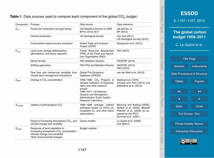
ESSDD5, 1107–1157, 2012


C. Le Quere et al.

Title Page



Tables Figures

J I

J I

Back Close

Full Screen / Esc



Discussion

Paper

|D

iscussionP

aper|

Discussion

Paper

|D

iscussionP

aper|

Table 1. Data sources used to compute each component of the global CO2 budget.

Component Process Data source Data reference

EFF Fossil fuel combustion and gas flaring UN Statistics Division to 2009BP for 2010–2011

UN (2012a, b)BP (2012)

Cement production US Geological Survey Van Oss (2011)US Geological Survey (2012)

Consumption-based country emissions Global Trade and AnalysisProject (GTAP)

Narayanan et al. (2012)

ELUC Land cover change (deforestation,afforestation, and forest regrowth)

Forest Resource Assessment(FRA) of the Food and Agricul-ture Organisation (FAO)

FAO (2010)

Wood harvest FAO Statistics Division FAOSTAT (2010)

Shifting agriculture FAO FRA and Statistics Division FAOSTAT (2010)FAO (2010)

Peat fires and interannual variability fromclimate-land management interactions

Global Fire EmissionsDatabase (GFED3)

van der Werf et al. (2010)

GATM Change in CO2 concentration 1959–1980: CO2 Program atScripps Institution of Oceanog-raphy and other researchgroups.1980–2011: US NationalOceanic and AtmosphericAdministration Earth SystemResearch Laboratory

Keeling et al. (1976)Conway and Tans (2012) andBallantyne et al. (2012)

SOCEAN Uptake of anthropogenic CO2 1990–1999 average: indirectestimates based on CFCs, at-mospheric O2, and other tracerobservations

Manning and Keeling (2006);McNeil et al. (2003); MikaloffFletcher et al. (2006) as as-sessed by the IPCCDenman et al. (2007)

Impact of increasing atmospheric CO2, andclimate change and variability

Ocean models Le Quere et al. (2009)and Table 3

SLAND Response of land vegetation to:Increasing atmospheric CO2 concentrationClimate change and variabilityOther environmental changes

Budget residual

1147





ESSDD5, 1107–1157, 2012


C. Le Quere et al.

Title Page



Tables Figures

J I

J I

Back Close

Full Screen / Esc



Discussion

Paper

|D

iscussionP

aper|

Discussion

Paper

|D

iscussionP

aper|

Table 2. Comparison of the processes included in the ELUC of the global carbon budget and theDGVMs. See Table 3 for model references.

CO2 budget VISIT ISAM-HYDE LPJmL LPJ-Bern

Deforestion, afforestation,forest regrowth after aban-donment of agriculture

yes yes yes yes yes

Wood harvest and forestdegradation

yes no yes no no

Shifting cultivation yes yes yes no no

Cropland harvest yes no no no yes

Peat fires from 1998 no no no no

Fire suppression for US only no no no no

Management-Climateinteractions

from 1998 no no no no

Climate change andvariability

no climate change ispresent but decadalmean response isused for regrowinguptake

climate variabilitypresent but notcorresponding toobserved years

yes yes

CO2 fertilisation no yes yes yes yes

Nitrogen dynamics no no yes no no

1148





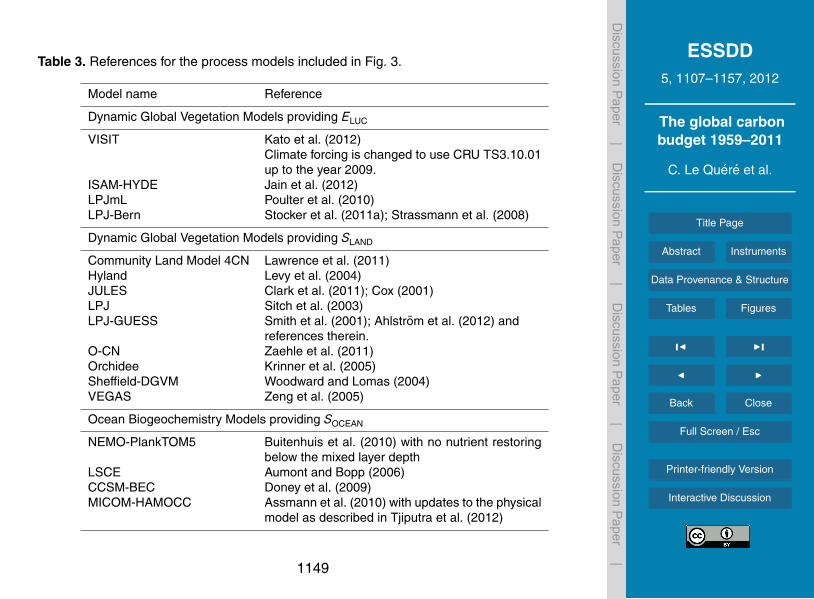
ESSDD5, 1107–1157, 2012


C. Le Quere et al.

Title Page



Tables Figures

J I

J I

Back Close

Full Screen / Esc



Discussion

Paper

|D

iscussionP

aper|

Discussion

Paper

|D

iscussionP

aper|

Table 3. References for the process models included in Fig. 3.

Model name Reference

Dynamic Global Vegetation Models providing ELUC

VISIT Kato et al. (2012)Climate forcing is changed to use CRU TS3.10.01up to the year 2009.

ISAM-HYDE Jain et al. (2012)LPJmL Poulter et al. (2010)LPJ-Bern Stocker et al. (2011a); Strassmann et al. (2008)

Dynamic Global Vegetation Models providing SLAND

Community Land Model 4CN Lawrence et al. (2011)Hyland Levy et al. (2004)JULES Clark et al. (2011); Cox (2001)LPJ Sitch et al. (2003)LPJ-GUESS Smith et al. (2001); Ahlstrom et al. (2012) and

references therein.O-CN Zaehle et al. (2011)Orchidee Krinner et al. (2005)Sheffield-DGVM Woodward and Lomas (2004)VEGAS Zeng et al. (2005)

Ocean Biogeochemistry Models providing SOCEAN

NEMO-PlankTOM5 Buitenhuis et al. (2010) with no nutrient restoringbelow the mixed layer depth

LSCE Aumont and Bopp (2006)CCSM-BEC Doney et al. (2009)MICOM-HAMOCC Assmann et al. (2010) with updates to the physical

model as described in Tjiputra et al. (2012)

1149





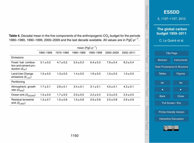
ESSDD5, 1107–1157, 2012


C. Le Quere et al.

Title Page



Tables Figures

J I

J I

Back Close

Full Screen / Esc



Discussion

Paper

|D

iscussionP

aper|

Discussion

Paper

|D

iscussionP

aper|

Table 4. Decadal mean in the five components of the anthropogenic CO2 budget for the periods1980–1989, 1990–1999, 2000–2009 and the last decade available. All values are in PgC yr−1.

mean (PgC yr−1)

1960–1969 1970–1989 1980–1989 1990–1999 2000–2009 2002–2011

Emissions

Fossil fuel combus-tion and cement pro-duction (EFF)

3.1±0.2 4.7±0.2 5.5±0.3 6.4±0.3 7.8±0.4 8.3±0.4

Land-Use Changeemissions (ELUC)

1.5±0.5 1.3±0.5 1.4±0.5 1.6±0.5 1.0±0.5 1.0±0.5

Partitioning

Atmospheric growthrate (GATM)

1.7±0.1 2.8±0.1 3.4±0.1 3.1±0.1 4.0±0.1 4.3±0.1

Ocean sink (SOCEAN) 1.5±0.5 1.7±0.5 2.0±0.5 2.2±0.4 2.3±0.5 2.5±0.5

Residual terrestrialsink (SLAND)

1.3±0.7 1.5±0.8 1.5±0.8 2.6±0.8 2.5±0.8 2.6±0.8

1150





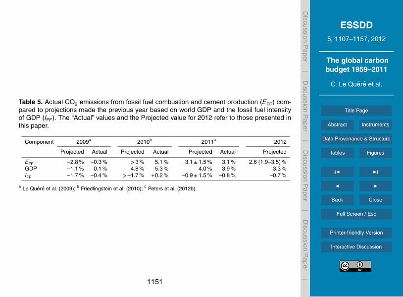
ESSDD5, 1107–1157, 2012


C. Le Quere et al.

Title Page



Tables Figures

J I

J I

Back Close

Full Screen / Esc



Discussion

Paper

|D

iscussionP

aper|

Discussion

Paper

|D

iscussionP

aper|

Table 5. Actual CO2 emissions from fossil fuel combustion and cement production (EFF) com-pared to projections made the previous year based on world GDP and the fossil fuel intensityof GDP (IFF). The “Actual” values and the Projected value for 2012 refer to those presented inthis paper.

Component 2009a 2010b 2011c 2012

Projected Actual Projected Actual Projected Actual Projected

EFF –2.8 % –0.3 % >3 % 5.1 % 3.1±1.5 % 3.1 % 2.6 (1.9–3.5) %GDP –1.1 % 0.1 % 4.8 % 5.3 % 4.0 % 3.9 % 3.3 %IFF –1.7 % –0.4 % >–1.7 % +0.2 % –0.9±1.5 % –0.8 % –0.7 %

a Le Quere et al. (2009); b Friedlingstein et al. (2010); c Peters et al. (2012b).

1151





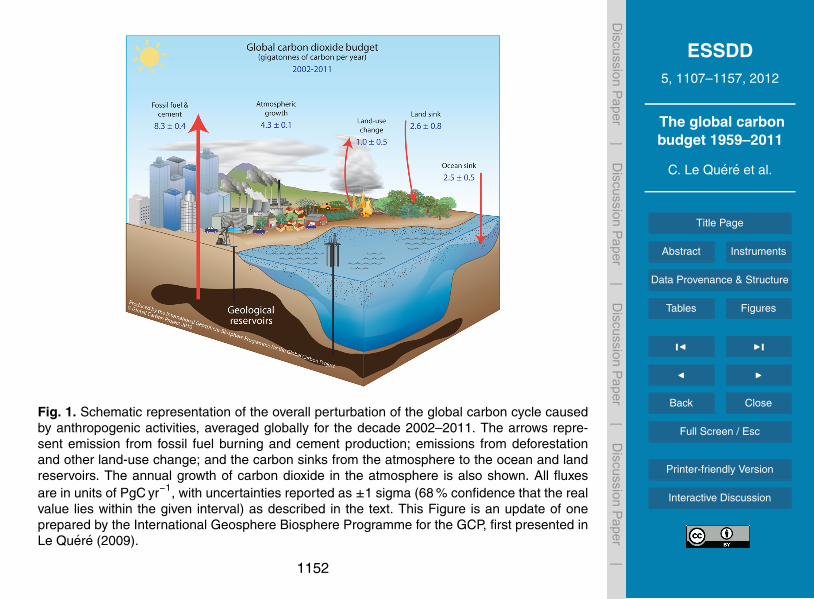
ESSDD5, 1107–1157, 2012


C. Le Quere et al.

Title Page



Tables Figures

J I

J I

Back Close

Full Screen / Esc



Discussion

Paper

|D

iscussionP

aper|

Discussion

Paper

|D

iscussionP

aper|

Fig. 1. Schematic representation of the overall perturbation of the global carbon cycle causedby anthropogenic activities, averaged globally for the decade 2002–2011. The arrows repre-sent emission from fossil fuel burning and cement production; emissions from deforestationand other land-use change; and the carbon sinks from the atmosphere to the ocean and landreservoirs. The annual growth of carbon dioxide in the atmosphere is also shown. All fluxesare in units of PgC yr−1, with uncertainties reported as ±1 sigma (68 % confidence that the realvalue lies within the given interval) as described in the text. This Figure is an update of oneprepared by the International Geosphere Biosphere Programme for the GCP, first presented inLe Quere (2009).

1152





ESSDD5, 1107–1157, 2012


C. Le Quere et al.

Title Page



Tables Figures

J I

J I

Back Close

Full Screen / Esc



Discussion

Paper

|D

iscussionP

aper|

Discussion

Paper

|D

iscussionP

aper|

Fig. 2. Combined components of the global carbon budget illustrated in Fig. 1 as a functionof time, for (top) emissions from fossil fuel combustion and cement production (EFF; grey) andemissions from land-use change (ELUC; brown), and (bottom) their partitioning among the atmo-sphere (GATM; light blue), land (SLAND; green) and oceans (SOCEAN; dark blue). All time-seriesare in PgC yr−1. Land-use change emissions include management-climate interactions fromyear 1997 onwards, where the line changes from dashed to full.

1153





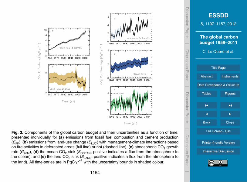
ESSDD5, 1107–1157, 2012


C. Le Quere et al.

Title Page



Tables Figures

J I

J I

Back Close

Full Screen / Esc



Discussion

Paper

|D

iscussionP

aper|

Discussion

Paper

|D

iscussionP

aper|

Fig. 3. Components of the global carbon budget and their uncertainties as a function of time,presented individually for (a) emissions from fossil fuel combustion and cement production(EFF), (b) emissions from land-use change (ELUC) with management-climate interactions basedon fire activities in deforested areas (full line) or not (dashed line), (c) atmospheric CO2 growthrate (GATM), (d) the ocean CO2 sink (SOCEAN, positive indicates a flux from the atmosphere tothe ocean), and (e) the land CO2 sink (SLAND, positive indicates a flux from the atmosphere tothe land). All time-series are in PgC yr−1 with the uncertainty bounds in shaded colour.

1154





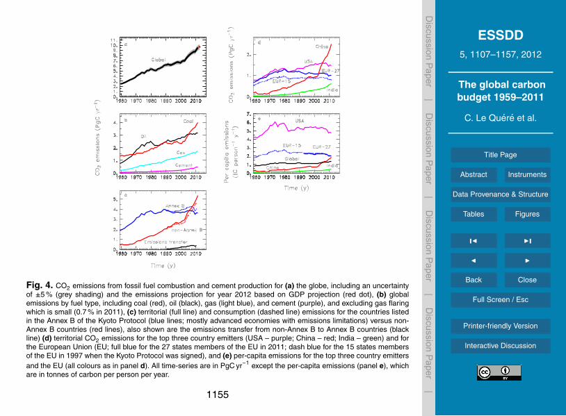
ESSDD5, 1107–1157, 2012


C. Le Quere et al.

Title Page



Tables Figures

J I

J I

Back Close

Full Screen / Esc



Discussion

Paper

|D

iscussionP

aper|

Discussion

Paper

|D

iscussionP

aper|

Fig. 4. CO2 emissions from fossil fuel combustion and cement production for (a) the globe, including an uncertaintyof ±5 % (grey shading) and the emissions projection for year 2012 based on GDP projection (red dot), (b) globalemissions by fuel type, including coal (red), oil (black), gas (light blue), and cement (purple), and excluding gas flaringwhich is small (0.7 % in 2011), (c) territorial (full line) and consumption (dashed line) emissions for the countries listedin the Annex B of the Kyoto Protocol (blue lines; mostly advanced economies with emissions limitations) versus non-Annex B countries (red lines), also shown are the emissions transfer from non-Annex B to Annex B countries (blackline) (d) territorial CO2 emissions for the top three country emitters (USA – purple; China – red; India – green) and forthe European Union (EU; full blue for the 27 states members of the EU in 2011; dash blue for the 15 states membersof the EU in 1997 when the Kyoto Protocol was signed), and (e) per-capita emissions for the top three country emittersand the EU (all colours as in panel d). All time-series are in PgC yr−1 except the per-capita emissions (panel e), whichare in tonnes of carbon per person per year.

1155





ESSDD5, 1107–1157, 2012


C. Le Quere et al.

Title Page



Tables Figures

J I

J I

Back Close

Full Screen / Esc



Discussion

Paper

|D

iscussionP

aper|

Discussion

Paper

|D

iscussionP

aper|

Fig. 5. Comparison of (top panel) CO2 emissions from land-use change (LUC), (middle panel)land CO2 sink (SLAND), and (bottom panel) ocean CO2 sink (SOCEAN) between the CO2 budgetvalues estimated here (black line), and those estimated from process models (Table 3; colouredlines). The thin dotted black lines in the top and middle panels are the model averages. TheLUC emissions from the CO2 budget estimate is dashed before year 1997 to highlight thestart of the satellite data from that year, as used to quantify the interannual variability frommanagement-climate interactions based on fire activities in deforested areas. For the oceanCO2 sink, the four models used in Le Quere et al. (2009) are shown in dark blue, while theupdated and models used to calculate interannual variability after 2008 are shown in pale blue.

1156





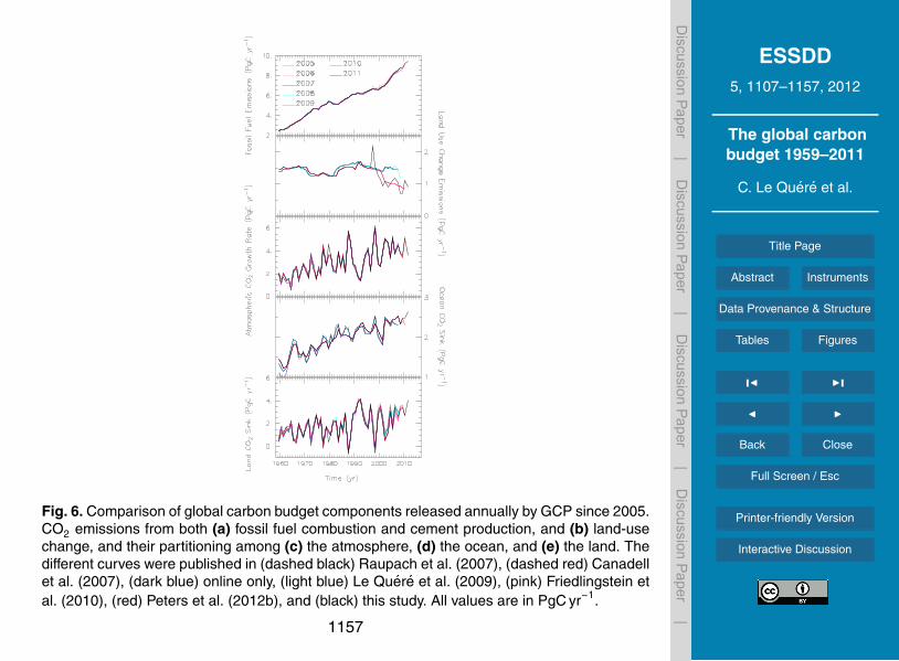
ESSDD5, 1107–1157, 2012


C. Le Quere et al.

Title Page



Tables Figures

J I

J I

Back Close

Full Screen / Esc



Discussion

Paper

|D

iscussionP

aper|

Discussion

Paper

|D

iscussionP

aper|

Fig. 6. Comparison of global carbon budget components released annually by GCP since 2005.CO2 emissions from both (a) fossil fuel combustion and cement production, and (b) land-usechange, and their partitioning among (c) the atmosphere, (d) the ocean, and (e) the land. Thedifferent curves were published in (dashed black) Raupach et al. (2007), (dashed red) Canadellet al. (2007), (dark blue) online only, (light blue) Le Quere et al. (2009), (pink) Friedlingstein etal. (2010), (red) Peters et al. (2012b), and (black) this study. All values are in PgC yr−1.

1157





Data J I Social - Copernicus.org

Documents

Transcript of Data J I Social - Copernicus.org