Data Evaluation for a Newly Developed Slack-Line Mooring ...

Data Evaluation for a Newly Developed Slack-Line Mooring Buoy Deployedin the Eastern Indian Ocean

IWAO UEKI

Research Institute for Global Change, Japan Agency for Marine-Earth Science and Technology, Yokosuka, Japan

NOBUHIRO FUJII

Marine Works Japan, Ltd., Yokohoma, Japan

YUKIO MASUMOTO AND KEISUKE MIZUNO

Research Institute for Global Change, Japan Agency for Marine-Earth Science and Technology, Yokosuka, Japan

(Manuscript received 17 August 2009, in final form 1 March 2010)

ABSTRACT

For the purpose of climate research and forecasting the Research Moored Array for African–Asian–

AustralianMonsoon Analysis and Prediction (RAMA) in the Indian Ocean has been planned. Development

of RAMA has been gradually accelerated in recent years as a multinational effort. To promote RAMA the

authors have developed a small size buoy system, which uses the slack-line mooring method, intended for the

easy handling of maintenance on a relatively small vessel. The authors have also conducted a field experiment

of the simultaneous deployment of new slack-line mooring and conventional taut-line mooring in the eastern

Indian Ocean. This paper describes the performance of the newly developed buoy system, especially the data

consistency against the taut-line mooring system, which is usually used for a tropical moored buoy array.

Although the slack-linemooringmethod has the advantage of downsizing the total mooring system, it also has

the disadvantage of having relatively large vertical shifts of installed sensors produced by a large migration of

the surface buoy. To offset this disadvantage to a certain extent, a data reconstruction method has been

developed and evaluated. Through the data comparison between both mooring systems, it is confirmed that

the reconstructed data of the newly developed buoy can basically capture the same features as that observed

with a conventional taut-line mooring system. The maximum mean difference of20.168C and the maximum

root-mean-square (RMS) difference of 0.588C for temperature appeared within the thermocline layer,

whereas themaximummean difference of 0.02 and themaximumRMSdifference of 0.09 for salinity appeared

within the mixed layer. Considering a distance of 8 n mi between the two moorings, these values are ac-

ceptable for regarding that the two moorings can observe same feature. Results of this study support the

introduction of various types of mooring systems for a multinational approach of RAMA and contribute to

the further progress of RAMA, climate research, and forecasting.

1. Introduction

The tropical buoy array, which consists of the Tropical

Atmosphere Ocean/Triangle Trans-Ocean Buoy Net-

work (TAO/TRITON) array in the Pacific, the Prediction

and Research Moored Array in the Tropical Atlantic

(PIRATA) in the Atlantic, and the Research Moored

Array for African–Asian–Australian Monsoon Analysis

and Prediction (RAMA) in the Indian Ocean, is an im-

portant component of several global earth observing

systems—such as the Global Ocean Observing System

(GOOS) and the Global Climate Observing System

(GCOS). These basin-scale tropical mooring arrays have

been designed to describe and monitor climate variability,

such as the El Nino–Southern Oscillation (ENSO) in the

Pacific. An advantage of using a mooring array is its ca-

pability to capture the short-term variability of the ocean

and the atmosphere associated with climate variability.

A highly developedmooring array is the TAO/TRITON

array in the Pacific. The data observed with TAO/

TRITONarray are used forENSOmonitoring, prediction,

Corresponding author address: Iwao Ueki, Japan Agency for

Marine-Earth Science and Technology, 2-15 Natsushima-cho,

Yokosuka 237-0061, Japan.

E-mail: [email protected]

JULY 2010 UEK I ET AL . 1195

DOI: 10.1175/2010JTECHO735.1

� 2010 American Meteorological SocietyUnauthenticated | Downloaded 12/25/21 10:26 AM UTC

and process study in associated mechanisms (McPhaden

et al. 1998; Kuroda and Amitani 2001). PIRATA, de-

veloped as a multinational array by Brazil, France, and

the United States, also provides useful information re-

garding the tropical Atlantic climate variability and its

prediction (Servain et al. 1998; Bourles et al. 2008).

Compared with arrays in the Pacific and the Atlantic,

RAMA in the Indian Ocean is still developing. The

Indian Ocean has important climate variability, such as

monsoon activity (Webster et al. 1998) and the Indian

Ocean Dipole (IOD) event (Saji et al. 1999; Webster

et al. 1999), which affects the local and world climate

through atmospheric teleconnections. RAMA is par-

ticularly effective for research and prediction of intra-

seasonal variability, such as theMadden–Julian oscillation

(MJO;Madden and Julian 1994; Lloyd and Vecchi 2010).

Despite the recognition of the societal and economic im-

pacts of climate variability in the Indian Ocean at pres-

ent, we do not have adequate observational data for

understanding the coupled ocean–atmosphere behavior.

The Climate Variability and Predictability (CLIVAR)/

GOOS Indian Ocean Panel (IOP) established an imple-

mentation plan for the sustained basin-scale IndianOcean

observing system (IndOOS), which consists of satellite-

based and in situ measurements (Meyers and Boscolo

2006; Masumoto et al. 2010). The satellite-based mea-

surements provide oceanic surface properties, such as

sea surface temperature, sea level, wind, rain, cloud, and

ocean color, whereas the in situ measurements provide

subsurface information. The in situ measurements cover

a variety of elements, such as the basin-scale mooring

array, Argo floats, surface drifters, expendable bathy-

thermograph (XBT) lines, and coastal tide gauge sta-

tions. RAMA, a component of IndOOS, is essential for

capturing the seasonal monsoon variability and intra-

seasonal disturbances. Simultaneous measurements for

oceanic and meteorological variables lead us to in-

vestigate the relationship and interaction between var-

iations in both the fields.

The main portion of the planned RAMA consists of

38 surface moorings, which measure subsurface tem-

perature, salinity, and mixed layer currents, and surface

meteorological variables. In addition to these surface

moorings, RAMA has eight subsurface acoustic Doppler

current profilers (ADCPs) and current-meter moorings

for subsurface and deep currents (Masumoto et al. 2005;

Sengupta et al. 2004;Murty et al. 2006). The array covers

major regions associated with the ocean–atmosphere

interaction in the Indian Ocean, such as the equatorial

waveguide; the Arabian Sea and the Bay of Bengal,

where intraseasonal and semiannual atmospheric forc-

ing is dominant; the eastern and western pole of IOD;

and the thermocline ridge near 108S. The array is de-

signed to capture the basin-scale pattern of oceanic and

atmospheric variability on intraseasonal to interannual

time scales. The mooring observations at fixed positions

are suitable for studying oceanic responses for atmo-

spheric disturbances such as theMJO, ocean–atmospheric

interactions, and mixed layer dynamics. In addition to

using the acquired data for studying the previously

mentioned scientific interest, the data are also used for

developing operational climate forecast models and

carrying out weather and climate prediction, ocean-

state monitoring, reanalysis, and satellite validation.

The lifetime of each mooring is basically 1 yr; there-

fore, annual replacement of the moorings is required.

By making reasonable assumptions, McPhaden et al.

(2006) estimated that a minimum of 142 days of ship

time per year is required tomaintain the completeRAMA

array. To solve this fundamental problem, a multina-

tional approach is required for securing financial resources

and ship time. At present, nations including Japan, the

TABLE 1. Observed parameters and depths of underwater sensors for m-TRITON and TRITONmoorings. Except temperature, salinity,

and pressure, each mooring has a current meter at a depth of 10 m.

m-TRITON TRITON

Level No. Depth (m) Parameter Depth (m) Parameter

1 1 Temperature, conductivity, pressure 1.5 Temperature, conductivity

2 10 Temperature, conductivity, pressure 25 Temperature, conductivity



5 60 Temperature, pressure 100 Temperature, conductivity




9 140 Temperature, pressure 250 temperature, conductivity

10 200 Temperature, pressure 300 Temperature, conductivity, pressure


12 500 Temperature, pressure 750 Temperature, conductivity, pressure

1196 JOURNAL OF ATMOSPHER IC AND OCEAN IC TECHNOLOGY VOLUME 27

Unauthenticated | Downloaded 12/25/21 10:26 AM UTC

United States, India, Indonesia, China, and France pro-

vide mooring equipment, ship time, logistic support, and

so on. The present status of RAMA is 54% complete,

with 25 of the 46 total mooring sites occupied at the end

of February 2010. The percentage increased gradually

compared with 47% at the end of 2008, reported by

McPhaden et al. (2009).

The Japan Agency for Marine-Earth Science and

Technology (JAMSTEC) deployed anADCP subsurface

mooring at 08908E in 2000 (Masumoto et al. 2005) and

two TRITON moorings at 58S, 958E and 1.58S, 908E in

2001 (Hase et al. 2008). These moorings became an ini-

tiation of the basin-scale IndianOceanmooring array. In

2005, JAMSTEC started a 5-yr program named the In-

dian Ocean Moored Buoy Network Initiative for Cli-

mate Studies (IOMICS) for promoting RAMA. In this

program, it is vital to develop a small size buoy system,

which will enable an easier mooring operation, reduce

maintenance costs, and enhance its capability for data

sampling and transmission. To reduce the surface buoy

size, the slack-linemooringmethod is adopted instead of

the taut-line mooring method for the TRITON buoy.

The two TRITON mooring sites described before were

replaced by the new buoy system named m-TRITON in

February 2008.

In this study, we evaluate the observed data acquired

by the newly developed m-TRITON buoy through a

field experiment for two types of mooringmethods—the

FIG. 1. Schematic representation of the m-TRITON mooring system.

FIG. 2. Schematic diagram of the difference between (left) taut-

line and (right) slack-linemoorings. Note that the shape ofmooring

lines for both buoys is not to scale to emphasize the different

concepts.



slack-line and taut-line methods—in the eastern equa-

torial Indian Ocean. The characteristics of RAMA as a

multinational effort and the installation of various types

of moorings will be considered. Therefore, consistency

in data quality among different mooring methods is cru-

cial. Section 2 describes the newly developedm-TRITON

buoy and the difference between slack-line and taut-line

moorings. Details of the field experiment and the be-

havior of the m-TRITON buoy are given in sections 3

and 4. In section 5, we discuss the interpolation method

used for the acquired data. Data evaluation through the

field experiment is described in section 6, and the results

are summarized in section 7.

2. Development of the m-TRITON buoy

To understand the mechanisms of the Indian Ocean’s

variation and the importance of its role with respect to

the global climate system, JAMSTEC has started two

surface moorings named TRITON at 1.58S, 908E and

58S, 958E in the eastern Indian Ocean since 2001 fol-

lowing the western Pacific TRITON moorings. The fo-

cus of the Indian Ocean TRITON moorings is the IOD

and oceanic response to atmospheric disturbances such

as MJO and monsoon. These TRITON moorings have

successfully provided information about the condition of

the eastern Indian Ocean, especially for the IOD event in

2006 and 2007 (Horii et al. 2007). Although the TRITON

buoy shows good performance as a climate-monitoring

buoy system, the relatively large buoy size (weight of

the surface float is 2400 kg and diameter is 2.4 m) re-

quires a large vessel for maintenance and hence a high

cost.

To promote the activities related to the Global Earth

Observation System of Systems (GEOSS), JAMSTEC

started the IOMICS program in 2005. One of the vital

portions of this program is the development of a new

buoy system. TheCLIVAR/GOOS IOP established some

recommendations for the development and maintenance

of the basin-scale mooring array in the Indian Ocean. In

the case of the observed variables, the required variables

are almost the same as for the present TRITONmoorings,

such as wind, air temperature, relative humidity, short-

wave radiation, barometric pressure, and precipitation

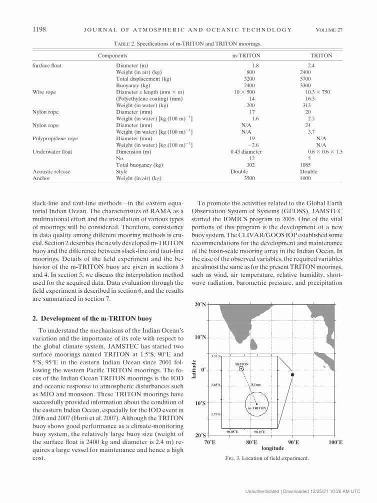
TABLE 2. Specifications of m-TRITON and TRITON moorings.

Components m-TRITON TRITON

Surface float Diameter (m) 1.8 2.4

Weight (in air) (kg) 800 2400

Total displacement (kg) 3200 5700

Buoyancy (kg) 2400 3300

Wire rope Diameter x length (mm 3 m) 10 3 500 10.3 3 750

(Polyethylene coating) (mm) 14 16.3

Weight (in water) (kg) 200 313

Nylon rope Diameter (mm) 17 20

Weight (in water) [kg (100 m)21] 1.6 2.5

Nylon rope Diameter (mm) N/A 24

Weight (in water) [kg (100 m)21] N/A 3.7

Polypropylene rope Diameter (mm) 19 N/A

Weight (in water) [kg (100 m)21] 22.6 N/A

Underwater float Dimension (m) 0.43 diameter 0.6 3 0.6 3 1.5

No. 12 5

Total buoyancy (kg) 302 1085

Acoustic release Style Double Double

Anchor Weight (in air) (kg) 3500 4000

FIG. 3. Location of field experiment.



for meteorological variables, and also the upper-ocean

temperature, salinity, and horizontal currents for the

physical oceanographic variables. However, the sam-

pling levels in the ocean are slightly different between

both, depending on the shallower mixed layer in the

Indian Ocean. The observed parameters and depths for

m-TRITON are partly modified according to the recom-

mendations, as listed in Table 1. Another key issue of

the recommendations is a multinational approach for

array maintenance. Although each mooring belonging

to RAMA will be deployed through national programs,

the coordination of these national efforts at an inter-

national level is essential for optimizing the utilization of

resources, such as ship time and mooring facilities, to

coordinate deployment schedules, maintainmeasurement

standards, and promote the free and open exchange of

data. We basically follow the recommendation on the

development of the m-TRITON mooring system. To

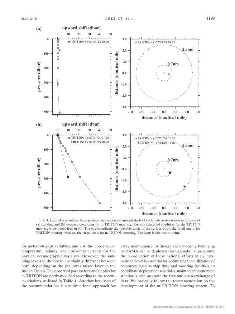
FIG. 4. Examples of surface buoy position and associated upward shifts of each underwater sensor in the case of

(a) standing and (b) declined conditions for m-TRITON mooring. The most declined condition for the TRITON

mooring is also described in (b). The circles indicate the movable circle of the surface buoy: the small one is for

TRITON mooring, whereas the large one is for m-TRITON mooring. The focus is the anchor point.



contribute to the multinational RAMA, our focus for

the new system development is concentrated on down-

sizing for the purpose of easy maintenance by smaller

vessels, which enables us to select from a wide range of

vessels for maintenance.

For this purpose, we have adopted a slack-linemooring

method for the m-TRITON system rather than the taut-

line mooring method used for the present TRITON sys-

tem. The basic concepts of our surface mooring are no

breaking off, no drifting with an anchor, and no sub-

merging the surface buoy. The slack-line mooring has a

relatively long mooring line, which is longer than the

water depth to reduce the tension along the mooring line.

A scope ratio, which is the ratio of the mooring line and

the water depth, of 1.3 is adopted for the m-TRITON

mooring system (Fig. 1). In the case of the same drag

force induced by currents, the tension along the moor-

ing line of a slack-linemooring is lower than that of taut-

line mooring because slack-line mooring allows a wider

range of surface buoy migration. Therefore, we can use

a small surface buoy, a thinner-diameter cable, and smaller

parts such as shackles, chains, and the anchor (Fig. 2).

The specifications of the m-TRITON and TRITON

mooring systems are listed in Table 2. Although the slack-

line mooring method has advantages for the downsizing

of the total system, it also has a disadvantage that un-

derwater sensors installed on the mooring line can ver-

tically move a large distance according to the larger

inclination of the mooring line as compared to that in

the case of the taut-line method. Therefore, we have to

observe the depth of each sensor and convert the ob-

served variables at each depth into those at the fixed

depth for the time series analysis. Because the data con-

version contains an error, which depends on the inter–

extrapolation method, verification is required.

3. Field experiment for data comparison

For the purpose of the verification of the performance

of a 1-yr mooring and data consistency between differ-

ent mooring methods, we conducted a field experiment

at 1.58S, 908E fromDecember 2006 to February 2008. In

the field experiment, two moorings by m-TRITON and

the present TRITON buoy were carried out. The dis-

tance between both moorings is approximately 8 n mi

(Fig. 3). The actual positions of both the moorings are

1842.989S, 90808.289E for m-TRITON and 1835.639S,90805.419E for TRITON.

In this study, we focus on the comparison between the

water temperature and salinity of both moorings. The

installed sensors for temperature and salinity are SBE-

37IM and SBE-39IM, manufactured by Sea-Bird Elec-

tronics, Inc, respectively. The nominal accuracies of

temperature and conductivity are 0.0028C and 0.0003

S m21, corresponding to a salinity of 0.002 at a conduc-

tivity level of around 6 S m21. Considering the calibra-

tion error of our sensor calibration system, the actual

accuracy of conductivity–salinity becomes (0.000 85 Sm21)/

(0.006) (Ando et al. 2005). These are the satisfactory

TABLE 3. Statistical values of the pressure observed with each

underwater sensor on m-TRITON mooring from 5 Dec 2006 to

6 Feb 2008.

Install

depth (m)

Statistical values of observed pressure (dbar)

Mean Std dev Min Max

10 9.73 0.13 8.47 10.18

20 19.66 0.18 18.13 20.40

40 39.66 0.35 36.04 40.61

60 59.21 0.52 53.22 60.25

80 78.13 0.76 69.37 79.63

100 99.14 1.02 87.90 100.58

120 118.72 1.29 104.66 120.41

140 138.60 1.56 121.56 140.49

200 198.25 2.38 172.79 200.73

310 307.49 4.09 264.50 311.65

510 503.55 7.91 455.85 511.71

FIG. 5. Time series of the surface buoy position (blue line) defined from the anchor point and

the observed pressure (red line) of the deepest sensor installed at 510 m.



temperature value of 0.028Cand salinity value of 0.02 for

the recommendation accuracy supposed by CLIVAR/

GOOS IOP. Each underwater sensor was installed at

the standard depth, which is different between both

moorings, of each mooring system as listed in Table 1.

The standard depth of the TRITON mooring was de-

signed to capture the thick mixed layer of the western

Pacific Ocean, and the same mooring was deployed in

the Indian Ocean. However, the standard depth of the

m-TRITON mooring is designed for maintaining con-

sistency, as in the case of RAMA. The data acquired by

the TRITON mooring is converted into values at the

standard depth of m-TRITON using a type of spline

interpolation method proposed by Akima (1970) for

comparison.

Although data comparison between both moorings

was planned for 1-yr moorings fromDecember 2006, the

TRITON buoy unfortunately drifted after July 2007

because of vandalism. Therefore, available data for the

comparison is approximately 6 months. The temporal

resolution of each underwater sensor is 10 min for the

internal record, and the hourly averaged data are trans-

mitted by the ARGOS satellite communication system.

Because the minimum requirement for temporal sam-

pling of the RAMAdata is hourly, we use the hourly data

for comparison.

4. Behavior of the m-TRITON mooring

The m-TRITONmooring for the field experiment has

a scope ratio of 1.3 for a water depth of 4700 m,meaning

that there is a total mooring line of 6100 m. Further, it

allows for a movable radius of 3900 m, corresponding to

approximately 2.1 n mi, for the surface buoy. The be-

havior of the surface buoy and each underwater sensor

are illustrated as examples of the standing and inclined

TABLE 4. List of CTD casts on buoy operation cruise around

1.58S, 908E.

Date Location Cruise code

14 Nov 2000 00859.959S, 90800.149E MR00-K07

14 Nov 2000 02800.019S, 90800.069E MR00-K07

23 Oct 2001 01840.339S, 89859.539E MR01-K05

23 Oct 2001 01859.969S, 89859.829E MR01-K05

30 Jul 2002 01835.959S, 90803.669E MR02-K04

30 Jul 2002 01839.259S, 90800.679E MR02-K04

30 Jul 2002 02800.019S, 90800.049E MR02-K04

12 Jul 2003 01840.059S, 90800.779E MR03-K03

12 Jul 2003 01835.299S, 90804.659E MR03-K03

13 Jul 2003 01859.819S, 89859.779E MR03-K03

10 Jul 2004 01840.339S, 89859.129E MR04–03

8 Aug 2005 01837.699S, 90802.139E MR05–03

10 Aug 2005 02800.079S, 89859.859E MR05–03

5 Dec 2006 01838.369S, 90800.409E MR06–05

8 Feb 2008 01840.799S, 90801.439E MR07–07

FIG. 6. (a) Temperature and (b) salinity profiles observed with 15 CTD casts conducted on the buoy operation

cruise from 2000 to 2007. The red line indicates the mean profile of all casts, and the closed circles on the y axes

represent the target depths for the buoy observation.



conditions in Fig. 4. For the standing condition, when the

surface buoy is located around the anchor point, each

underwater sensor is located at the appropriate depths,

which are the nominal install depths of 1, 10, 20, 40, 60,

80, 100, 120, 140, 200, 310, and 510 m. It should be noted

that the two deeper sensors are installed below the tar-

get depths of 300 and 500 m because of the consider-

ation for the upward shift of underwater sensors. On the

other hand, the positions of underwater sensors become

shallower with an increase in the depth for the inclined

condition. In the case of the most declined condition,

the upward shifts of each underwater sensor for the

m-TRITON mooring are approximately twice as large

as those for TRITON mooring.

The statistical values for the observed pressure of

each underwater sensor during the mooring period from

December 2006 to February 2008 are listed in Table 3.

It should be noted that a pressure value in decibars at

a certain depth in the upper layer of the eastern Equa-

torial Indian Ocean is approximately 0.6% larger than

a depth value in meters. Considering the marking error

for the installation depth of each sensor on a wire rope,

we can regard the maximum value of the observed pres-

sure as the realistic installation depth. Except for the

sensor installed at a depth of 510 m, differences between

the observed mean and the installed depth of each

sensor are within a few decibars. The values of standard

deviation increase with an increase in depth. Consider-

ing an accuracy of 1.5 dbar for the pressure measure-

ment, effects of slack-line mooring appeared below 80 m.

The percentage of pressure values within themean plus–

minus accuracy in the total period are more than 95%

above 80 m, around 90% in the thermocline layer from

80 to 140 m, and less than 65% below 140 m. These

values imply that an effect of slack-line mooring cannot

be ignored, especially in a deeper layer. For the deepest

sensor installed at 510 m, the mean observed pressure is

503.6 dbar with a standard deviation of 7.9 dbar and the

maximum upward shift indicates approximately 55 dbar.

This high variability is caused by the variation in a tilt of

the mooring line, and it is a characteristic of the slack-

line mooring method.

The relationship between the surface buoy position

defined from the anchor point and the deepest sensor

depth is shown in Fig. 5. The anchor point is detected by

acoustical triangulation after buoy deployment, and the

surface buoy position is calculated by the ARGOS sys-

tem. The observed pressure has the tendency to de-

crease when the surface buoy is away from the anchor

point. The lowest observed pressure under 480 dbar ap-

peared in January 2007, and the longest distance from the

anchor point to the surface buoy was recorded at that

FIG. 7. Profile of the vertical gradient for temperature calculated from 15 CTD casts: (a) mean and (b) std dev. (c),(d) As in (a),(b), but

for salinity.



time. Although a tilt of the mooring line is also affected

by the vertical structure of ocean currents, the upward

shifts of each underwater sensor are mainly governed by

the surface buoy position.

5. Reconstruction of standard-level data

As described in the previous section, the vertical po-

sitions of each sensor installed on the m-TRITON

mooring have a relatively large variation, especially the

deeper sensors, because of the adoption of the slack-line

mooring method. As a result, the observed temperature

and salinity include effects of sensor position shifts in

addition to temporal variation. It should be noted that

we concentrate on the effects of the vertical shifts of in-

stalled sensors because the horizontal gradients of tem-

perature and salinity are relatively small compared with

the vertical gradients of these variables, except the sa-

linity front caused by a low-salinity patch.

Before the development of the m-TRITON buoy, we

deployed TRITON buoys at the same sites from 2000

and conducted 15 CTD casts around 1.58S, 908E during

buoy operation cruises (Table 4). Although 15 casts are

insufficient to describe the nature of variability for the

temperature and salinity at the site, we can confirm the

basis of the vertical structure of temperature and salin-

ity from these vertically high-resolution data. Figure 6

shows the temperature and salinity profiles observed

with CTD casts around 1.58S, 908E. Although the ther-

moclines appeared to have a relatively wide range from

60 to 120 dbar, a large difference among the casts was

related to the variations in the mixed layer thickness and

sharpness of the thermocline. Compared with the value

in the case of the thermocline layer, the difference above

40 dbar and below 200 dbar was relatively small. With

respect to salinity profiles, there was a salinity maximum

between 60 and 120 dbar. Basically, a layer of uniform

salinity was recognized near the sea surface; however, its

thickness varied largely. Moreover, the shallow halo-

cline appeared when the sea surface salinity was low.

The vertical gradient of temperature and salinity cal-

culated from the CTD casts are also shown in Fig. 7.

In the case of temperature, large gradients appeared

around the thermocline, and the maximum values of the

mean and standard deviation of the 15 casts were20.738and 0.938C dbar21. Meanwhile, large gradients for sa-

linity appeared above and below the salinity maximum.

The maximum vertical gradient appeared at 92 dbar,

and the values of the mean and standard deviation of

the 15 casts in this case were 0.03 and 0.12 dbar21,

FIG. 8. (a) Temperature and (b) salinity profiles observed with the CTD cast and m-TRITON mooring after

deployment. The solid lines indicate the CTD cast data, and the blue and red circles indicate the raw and the

reconstructed standard-level data, respectively.



respectively. The accuracy of the pressure sensor in-

stalled in the m-TRITON mooring was 1.5 dbar; there-

fore, the observational error for temperature and salinity

can exceed 1.108C and 0.05 at the depth at which the

maximum vertical gradient appeared. In addition to this

observational error, the vertical shifts of the installed

sensors caused by the slack-line mooring method led to

an additional error, if we considered the nominal target

depth as the correct depth without any correction.

Although each underwater sensor measures pressure,

for convenient use of the observed temperature and

salinity, raw data should be reconstructed into standard-

level data by an appropriate procedure, which reduces

the misinterpretation of the observational error caused

by the effects of the vertical shifts of the installed sen-

sors. The standard levels are defined by the target depths

of 1, 10, 20, 40, 60, 80, 100, 120, 140, 200, 300, and 500 m

for temperature and 1, 10, 20, 40, and 100 m for salinity—

these levels are recommended by CLIVAR/GOOS IOP.

Basically, we applied the Akima spline method proposed

byAkima (1970) for the reconstruction. TheAkima spline

method is a continuously differentiable subspline inter-

polation. It is built from piecewise third-order poly-

nomials and has an advantage of avoiding the typical

spline overshooting that occurs when the behavior of

the spline points is nonpolynomic. Because all under-

water sensors measure pressure, we can acquire 12 sets

of (P, T) pairs and 5 sets of (P, S) pairs. From these pairs

we get temperature and salinity profiles by applying the

Akima spline method, and temperature and salinity at

standard levels are extracted. For the bottom level, we

used the linear inter–extrapolation method instead of the

Akima spline method to avoid relatively large errors, de-

pending on how low was the resolution of measurements

in the vertical.

To confirm the normal operation of each underwater

sensor, we conducted a CTD cast near the m-TRITON

mooring when the deployment was completed. The ac-

quired profiles could be used for confirming the re-

constructionmethod. Figure 8 indicates the temperature

and salinity profiles at 1841.409S, 90810.289E, which

corresponds to a 4.7-km northeast point from the

m-TRITON mooring. The raw and reconstructed data

observed with the m-TRITON mooring are also shown

in Fig. 8. For the reconstruction of standard-level data of

the deepest level, corresponding to 500 m for tempera-

ture and 100 m for salinity, the deepest sensor may lo-

cate shallower than the deepest standard level because

of the inclined mooring line. In fact, in the case of this

comparison with the CTD cast, the observed pressure

of the deepest sensor for the salinity was 98.8 dbar. In

this case, the reconstruction of standard-level data for

100-dbar salinity was carried out by using linear extrap-

olation instead of the Akima spline method. Except the

sea surface salinity, the reconstructed data including

the deepest level were consistent with the CTD cast data

FIG. 9. Mean profiles of (a) temperature and (b) salinity calculated from 15 CTD casts with the observed pressure

variation range corresponding to minimum–maximum range from 5 Dec 2006 to 6 Feb 2008. The closed circles

indicate values at standard levels.



and the raw data in this comparison. A large sea surface

salinity difference between m-TRITON and CTD cast

observations might be caused by the relationship be-

tween the small horizontal structure of a low-salinity

patch and the difference between both the observation

points. We do not expect such sharp gradients at deeper

levels; therefore, we have to pay attention to the re-

construction of the deepest-level data. Although the

vertical gradient of temperature between 300 and 500 m

was relatively small in the equatorial Indian Ocean, the

salinity between 40 and 100 mwas quite large because of

the existence of a high-salinity core at around 100 m.

Therefore, the reconstructed salinity data for 100 m

might contain a relatively large error because of the po-

sition of the salinity maximum.

Although the validity of the adopted reconstruction

method was tested through the comparison between the

observed data with the m-TRITON mooring and the

CTD cast conducted just after deployment, the slack-

line mooring effect was not dominant in this situation;

the observed pressure of each sensor was almost equiv-

alent to that of the nominal target depth. Therefore, by

using the past 15 CTD casts presented previously, we

conducted a virtual test for the evaluation of the in-

terpolation method by simulating the slack-line effect.

The virtual test was carried out as follows. First, we

gathered temperature and salinity data at virtual ob-

served levels, which were defined by 14-month statistics

of the observed pressure described in section 3 from

each CTD cast. The virtual observed levels were set up

for three test cases: virtual observed pressure had values

of mean minus standard deviation, mean plus standard

deviation, and minimum. Then, we reconstructed the

standard-level data from the virtually observed data us-

ing the adopted method. Finally, the standard-level data

were compared with the real-value data, which were

gathered at each nominal standard level from the origi-

nal CTD cast. This procedure was repeated for 15 CTD

casts for each case.

Figure 9 indicates the mean temperature and salinity

profiles calculated from 15 CTD casts with minimum

TABLE 5. Error estimation of virtual test for temperature, with

values of the 14-month observed mean minus the standard de-

viation as the virtual observed pressure. The OE is misleading

when we regard the observed data as the standard-level data

without any correction, and the RE is defined as the difference

between the reconstructed data and the real data at the standard

level.

Standard

level (m)

Temperature

at standard

level (8C)Pressure

(dbar)

OE (8C) RE (8C)

Mean

Std

dev Mean

Std

dev

10 29.10 9.60 0.00 0.00 0.00 0.00

20 29.11 19.48 0.00 0.01 0.00 0.01

40 29.08 39.32 0.00 0.01 0.00 0.01

60 28.94 58.69 0.02 0.04 0.00 0.03

80 27.41 77.37 0.29 0.42 0.08 0.21

100 25.27 98.12 0.27 0.34 20.08 0.27

120 18.64 117.44 0.87 0.98 0.34 0.76

140 16.32 137.04 0.18 0.16 20.05 0.20

200 13.15 195.87 0.15 0.12 0.06 0.12

300 11.33 303.41 20.04 0.03 0.00 0.04

500 9.60 495.64 0.02 0.02 20.01 0.02

TABLE 6. As in Table 5, but with values of the 14-month ob-

served mean plus the standard deviation as the virtual observed

pressure.

Standard

level (m)

Temperature

at standard

level (8C)Pressure

(dbar)

OE (8C) RE (8C)

Mean

Std

dev Mean

Std

dev

10 29.10 9.86 0.00 0.00 0.00 0.00

20 29.11 19.84 0.00 0.00 0.00 0.00

40 29.08 40.01 0.00 0.00 0.00 0.00

60 28.94 59.74 0.00 0.00 0.00 0.00

80 27.41 78.89 0.07 0.10 0.01 0.06

100 25.27 100.16 0.00 0.00 0.00 0.00

120 18.64 120.01 0.00 0.00 0.00 0.00

140 16.32 140.16 0.00 0.00 0.00 0.00

200 13.15 200.64 20.02 0.01 0.01 0.02

300 11.33 311.58 20.15 0.09 0.00 0.13

500 9.60 511.47 20.06 0.05 0.03 0.05

TABLE 7. As in Table 5, but with the minimum values of observed

pressure within 14 months as the virtual observed pressure.

Standard

level (m)

Temperature

at standard

level (8C)Pressure

(dbar)

OE (8C) RE (8C)

Mean

Std

dev Mean

Std

dev

10 29.10 8.47 0.01 0.02 0.01 0.02

20 29.11 18.13 0.00 0.02 0.00 0.01

40 29.08 36.04 0.01 0.02 0.00 0.01

60 28.94 53.22 0.08 0.16 20.09 0.23

80 27.41 69.37 1.01 1.48 0.16 0.33

100 25.27 87.90 1.59 1.39 20.08 0.44

120 18.64 104.66 5.74 3.42 20.06 0.26

140 16.32 121.56 1.86 0.65 20.14 0.86

200 13.15 172.79 1.02 0.25 0.21 0.19

300 11.33 264.50 0.45 0.25 20.02 0.20

500 9.60 455.85 0.32 0.09 20.10 0.13

TABLE 8. As in Table 7, but for salinity.

Standard

level (m)

Salinity at

standard

level

Pressure

(dbar)

OE RE

Mean

Std

dev Mean

Std

dev

10 34.48 8.47 20.01 0.02 0.00 0.01

20 34.53 18.13 20.01 0.01 0.00 0.01

40 34.61 36.04 20.02 0.03 0.00 0.02

100 35.11 87.90 20.07 0.16 0.03 0.21



and maximum pressure values observed in 14 months.

As shown in these profiles, the vertical shifts of each

sensor produced a mismatch between the target depth

and the realistic depth, especially at deeper levels. In

addition to the deeper levels, this mismatch might pro-

duce misleading observed data at the depth of large

vertical gradient levels, such as near the thermocline

and halocline.

As shown in the previous section, the vertical shifts of

the sensors installed from near the sea surface to 60 m

were small; therefore, the test is concentrated on the

sensors installed 80 m and below. In addition to the

evaluation of the reconstruction method, we calculated

the errors defined as original errors (OEs), which were

caused bymisleading data if we considered the observed

data at the virtual observed levels as the standard-level

data without any correction. Results from this calcula-

tion demonstrated the need for data reconstruction.

In the case of having values of a 14-monthmeanminus

standard deviation as the virtual observed pressures, the

largest slack-line effect on the temperature data was

recognized at the standard level of 120 m, whereas

the largest upward shift appeared on the sensor in-

stalled at 510 m (Table 5). In the case of temperature,

the OEs of the mean and standard deviation of the

15 CTD casts were 0.878 and 0.988C, The largest slack-

line effect on the salinity data appeared at the standard

level of 100 m, and the OEs of the mean and standard

deviation of the 15 CTD casts at the level were 20.01

and 0.03. The reconstruction errors (REs) derived

from the comparison between the reconstructed and

the real data are also listed in Table 5. The REs were

relatively small against the OEs. The largest value of

REs for the mean and standard deviation of the 15 CTD

casts in the case of temperature at the standard level of

120 m were 0.348 and 0.768C. The largest value of REs

for the mean and standard deviation of the 15 CTD

casts in the case of salinity at the standard level of 100 m

were 0.00 and 0.03, which were small and comparable

to OEs.

FIG. 10. Time–depth diagram of temperature observed with (a) m-TRITON and (b) TRITON

moorings.



The test where the values of the 14-month mean plus

standard deviation was considered to be the virtual ob-

served pressures represented an almost standing condi-

tion of mooring; therefore, only two sensors installed at

310 and 510 m largely departed from the standard level.

It should be noted that these sensors are installed at the

depth of 10 m below the standard level to reduce slack-

line effect for temperature data. In this case, the largest

value of the OEs for the mean and standard deviation of

the 15 CTD casts appeared at the standard level of

300 m, and the values were20.158 and 0.098C (Table 6).

The values of REs for the mean and standard deviation

of the 15 CTD casts for this level were relatively small

(0.008 and 0.138C), which is the same as in the previous

case.

The most prominent case for the slack-line effect

appeared in the case with the minimum values of ob-

served pressure within 14 months served as the virtual

observed pressure. In the case of temperature, the largest

value of the OEs for the mean and standard deviation of

the 15 CTD casts was recognized at the standard level of

120 m, as in the first case. However, these values were

relatively large (5.748 and 3.428C; Table 7). In addition

to these largest values, relatively large values of the OEs

for the mean and standard deviation of the 15 CTD casts

appeared below the standard level of 60 m. The values

of REs for the mean and standard deviation of the

15 CTD casts at the standard level of 120 m were20.068and 0.218C, and the largest values of 0.198C for the mean

of the 15 CTD casts appeared at the standard level of

200 m. In the case of salinity, the OEs for the mean of

the 15 CTD casts at all standard levels were less than

20.01 (Table 8), and the smallest value of 20.07 with

a standard deviation of 0.16 was observed at the stan-

dard level of 100 m. Although the REs were relatively

small compared with those of OEs, as shown in the case

of temperature, the largest value of 0.03 for the mean

of the 15 CTD casts and that of 0.21 for the standard

FIG. 11. Time series of temperature observed with (a) m-TRITON and (b) TRITON

moorings at 40 m, and (c) its difference (m-TRITON temperature minus TRITON tempera-

ture). (d) Low-pass-filtered (25-h running mean) difference is also indicated. The observed

temperature is reconstructed into standard-level data.



deviation at the standard level of 100 m suggested a

difficulty in the reconstruction for the bottom level when

the slack-line effect was significant.

As shown in the results from the virtual test, OEs at

the standard level near the thermocline and halocline

increased. This result indicates a need for the data re-

construction of the standard-level data. On the other

hand, REs were relatively small even near the thermo-

cline and halocline. The maximum value of RE (0.168C)near the thermocline, corresponding to 80 m with the

minimum values of observed pressure within 14 months,

was less than the observation error (1.108C) estimated

from the pressure sensor accuracy. In the case of salinity,

the maximum value of RE (0.03) at the standard level of

100 m with the minimum values of observed pressure

within 14 months was equivalent to the observation

error (0.05).

6. Data comparison between two types of mooringsystems

When the slack-line mooring method was adopted for

the m-TRITON buoy, relatively large vertical shifts of

the installed sensors were coincident with the down-

sizing of the total mooring system. However, they could

be reduced by using an appropriate procedure, as dem-

onstrated in the previous section. In this section, we

confirm the data consistency between different mooring

methods through the field experiment described in sec-

tion 3. We have to pay attention to the difference in the

observation levels between the both moorings in the

data comparison. It should be noted that the recon-

structed m-TRITON data is used for this analysis.

In general, temporal variations in the vertical struc-

ture for temperature at both sites show almost the same

features, especially thermocline variation; however, there

are notable differences in the detailed structure, such

as mixed layer thickness (Fig. 10). To clarify the details,

we attempted a time series comparison between both

the buoys in three classified ranges: in the mixed layer

(40 m), in the thermocline (100 m), and below the ther-

mocline (300 m). It should be noted that the TRITON

temperature at 40 m was reconstructed by using the

Akima spline method because of the lack of observation

data at this depth. The available data for comparison

were acquired within almost 6 months from 5December

2006 to 16 June 2007.

At the depth of 40 m, themean difference (m-TRITON

minus TRITON) and root-mean-square (RMS) differ-

ence for temperature were 0.128 and 0.528C (Fig. 11).

The RMS difference decreased when we used a 25-h

running-mean filter as a low-pass filter, which suggested

an effect of a spatial phase difference in high-frequency

signals caused by a distance of 8 n mi between the two

buoys. The difference increased as the m-TRITON tem-

perature was higher than the TRITON temperature

in the middle of January and from February to March

2007 when the temperature rapidly decreased. It was

suggested from the time–depth diagram of the temper-

ature observed with both the moorings (Fig. 12) that the

difference was caused by a difference in the vertical res-

olution of the observation levels. The TRITON mooring

could not capture a detailed structure of the surface

mixed layer, especially near the bottom, which appeared

from 40 to 60 m.

At the depth of 100 m, the mean difference and

RMS difference in temperature were20.168 and 0.588C(Fig. 13). The m-TRITON temperature was relatively

lower than the TRITON temperature until the end of

February 2007, and then the difference decreased until

the beginning of April 2007. The amplitude of the dif-

ference increased after the beginning of April 2007.

This depth corresponds to the thermocline layer on av-

erage; therefore, the temperature variation was probably

affected by ocean dynamics forced by the sea surface

wind.

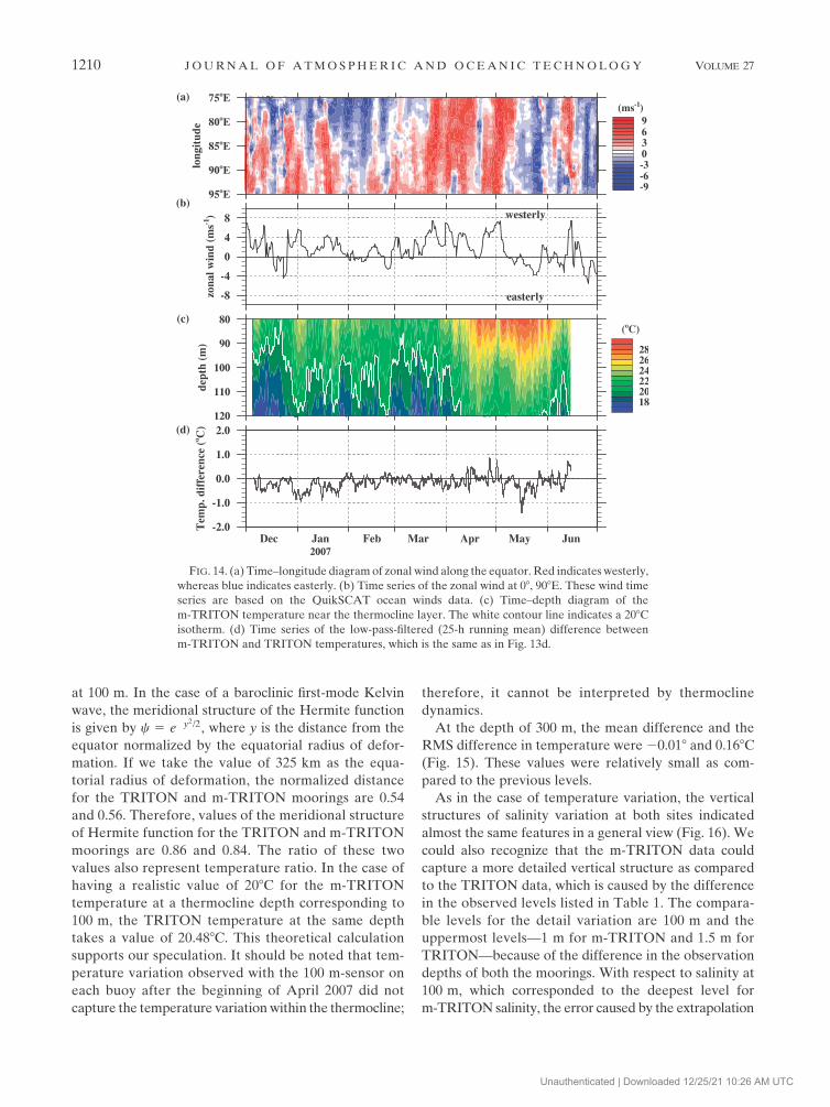
The time series of the equatorial zonal wind with the

time–depth diagram of temperature acquired with the

m-TRITON buoy is shown in Fig. 14. If we considered

a 208C isotherm as an index for thermocline variation, it

FIG. 12. Time–depth diagram of the upper-layer temperature

observed with (a) m-TRITON and (b) TRITON moorings from

Feb to Mar 2007. The closed circles indicate nominal observed

levels.



is seen that the thermocline depth changed considerably

until the end of February 2007, and it was then located

around 100 m until the first half of April 2007. The de-

velopment of themixed layer was found after themiddle

of April 2007, and the sensor installed around 100-m

depth captured the temperature variation within the

mixed layer. With respect to the wind variation, basi-

cally, westerly winds were dominant in the equatorial

region at 908E. For the spatial property of winds, the

zonal scales of thewesterly windswidened duringMarch–

April 2007. With respect to the time scale of wind varia-

tion, intraseasonal signals were recognized through the

entire observation period.

The oceanic response against the local westerly wind

near the equator was the Ekman transport to the equator

and the deepening of the thermocline. The relationship

between the observed vertical motion of the thermo-

cline and the zonal wind variation near the buoy position

was consistent until the end of February 2007—when

the westerly was dominant, the thermocline deepened.

However, the relationship become inconsistent from the

end of February to the middle of April 2007—vertical

motions of the thermocline became small, whereas the

local wind variation was not so different 1 month before.

This feature might be concerned with the upwelling

Kelvin waves exited by the easterly wind at the far-west

region around 758E. After the middle of April 2007, the

westerly had a large zonal scale; therefore, in addition

to the local wind, the downwelling Kelvin waves exited

by the westerly wind in the far-west region might sup-

port the remarkable deepening of the thermocline at the

observed site.

A large temperature difference between both the

buoys appeared until the end of February 2007 when

the thermocline was located between 80 and 120 m and

became relatively deeper, suggesting effects of the

westerly wind forcing.When the westerly was dominant,

the downwelling Kelvin waves exited near the equator.

Therefore, the influence of the downwelling was more

effective on the northern TRITON buoy as compared to

the southern m-TRITON buoy; the TRITON tempera-

ture became higher than the m-TRITON temperature

FIG. 13. As in Fig. 11, but for 100 m.



at 100 m. In the case of a baroclinic first-mode Kelvin

wave, the meridional structure of the Hermite function

is given by c 5 e�y2/2, where y is the distance from the

equator normalized by the equatorial radius of defor-

mation. If we take the value of 325 km as the equa-

torial radius of deformation, the normalized distance

for the TRITON and m-TRITON moorings are 0.54

and 0.56. Therefore, values of the meridional structure

of Hermite function for the TRITON and m-TRITON

moorings are 0.86 and 0.84. The ratio of these two

values also represent temperature ratio. In the case of

having a realistic value of 208C for the m-TRITON

temperature at a thermocline depth corresponding to

100 m, the TRITON temperature at the same depth

takes a value of 20.488C. This theoretical calculation

supports our speculation. It should be noted that tem-

perature variation observed with the 100 m-sensor on

each buoy after the beginning of April 2007 did not

capture the temperature variationwithin the thermocline;

therefore, it cannot be interpreted by thermocline

dynamics.

At the depth of 300 m, the mean difference and the

RMS difference in temperature were20.018 and 0.168C(Fig. 15). These values were relatively small as com-

pared to the previous levels.

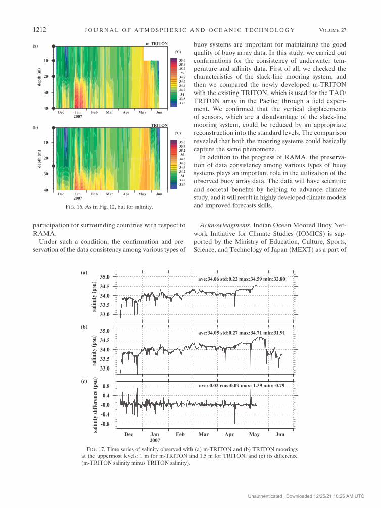
As in the case of temperature variation, the vertical

structures of salinity variation at both sites indicated

almost the same features in a general view (Fig. 16). We

could also recognize that the m-TRITON data could

capture a more detailed vertical structure as compared

to the TRITON data, which is caused by the difference

in the observed levels listed in Table 1. The compara-

ble levels for the detail variation are 100 m and the

uppermost levels—1 m for m-TRITON and 1.5 m for

TRITON—because of the difference in the observation

depths of both the moorings. With respect to salinity at

100 m, which corresponded to the deepest level for

m-TRITON salinity, the error caused by the extrapolation

FIG. 14. (a) Time–longitude diagramof zonal wind along the equator. Red indicates westerly,

whereas blue indicates easterly. (b) Time series of the zonal wind at 08, 908E. These wind time

series are based on the QuikSCAT ocean winds data. (c) Time–depth diagram of the

m-TRITON temperature near the thermocline layer. The white contour line indicates a 208Cisotherm. (d) Time series of the low-pass-filtered (25-h running mean) difference between

m-TRITON and TRITON temperatures, which is the same as in Fig. 13d.



for the reconstruction of standard-level data increased

when the mooring system was declined. Therefore, we

paid attention to buoy behavior for the comparison.

At the depth of the uppermost levels, the mean dif-

ference and RMS difference in salinity were 0.02 and

0.09 (Fig. 17). The spatial and temporal small scales of

the low surface salinity patch distribution, which was ob-

served in the Pacific warm pool by Soloviev and Lukas

(1996), might reflect this small mean difference and the

relatively large RMS difference.

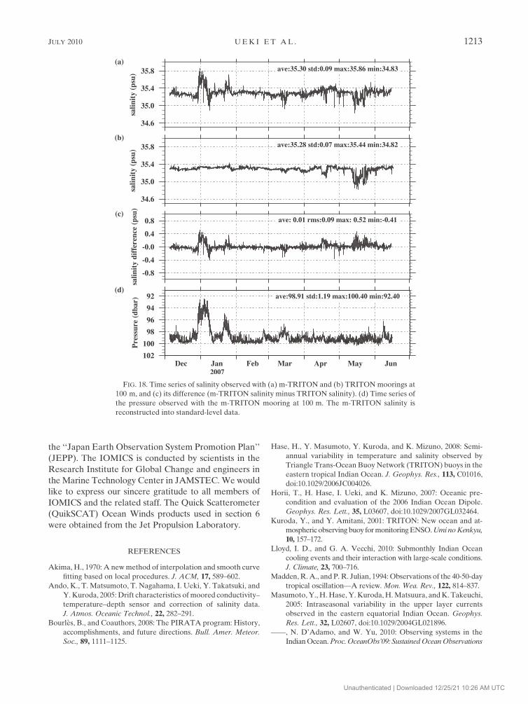
At the depth of 100 m, the mean difference and RMS

difference in salinity were 0.01 and 0.09 (Fig. 18). These

values were not so different from those in the uppermost

levels. However, there were some eventual signals as-

sociated with the pressure variation of the m-TRITON

sensor. These signals were caused by the data reconstruc-

tion method described in section 5 and produced an arti-

ficial error. Therefore, the actual RMS difference might

be reduced.

As described earlier, both buoys basically captured

the same signals, and it was suggested that the observed

differences were produced by the differences in the

mooring points and observation depths.

7. Concluding remarks

The progress of RAMA for understanding large-scale

ocean–atmosphere interaction phenomena, such as IOD

events, ocean dynamics, and climate variability in the

Indian Ocean, has been accelerated in the past 5 yr. A

fully developed RAMA will contribute to climate study

and operational activities for weather and climate fore-

casts, but it is still in the developing stage. To promote

the completion of RAMA, we developed a new slack-

line mooring buoy system, which facilitates the down-

sizing of the complete system for the purpose of easy

handling during operation. Because a multinational

effort is required for the progress of RAMA, the in-

stallation of various types of buoy systems are ex-

pected. Our new buoy system can become one such

system. Because this downsized system allows us to

select from a wide range of vessels, it leads to easy

FIG. 15. As in Fig. 11, but for 300 m.



participation for surrounding countries with respect to

RAMA.

Under such a condition, the confirmation and pre-

servation of the data consistency among various types of

buoy systems are important for maintaining the good

quality of buoy array data. In this study, we carried out

confirmations for the consistency of underwater tem-

perature and salinity data. First of all, we checked the

characteristics of the slack-line mooring system, and

then we compared the newly developed m-TRITON

with the existing TRITON, which is used for the TAO/

TRITON array in the Pacific, through a field experi-

ment. We confirmed that the vertical displacements

of sensors, which are a disadvantage of the slack-line

mooring system, could be reduced by an appropriate

reconstruction into the standard levels. The comparison

revealed that both the mooring systems could basically

capture the same phenomena.

In addition to the progress of RAMA, the preserva-

tion of data consistency among various types of buoy

systems plays an important role in the utilization of the

observed buoy array data. The data will have scientific

and societal benefits by helping to advance climate

study, and it will result in highly developed climatemodels

and improved forecasts skills.

Acknowledgments. Indian Ocean Moored Buoy Net-

work Initiative for Climate Studies (IOMICS) is sup-

ported by the Ministry of Education, Culture, Sports,

Science, and Technology of Japan (MEXT) as a part of

FIG. 16. As in Fig. 12, but for salinity.

FIG. 17. Time series of salinity observed with (a) m-TRITON and (b) TRITON moorings

at the uppermost levels: 1 m for m-TRITON and 1.5 m for TRITON, and (c) its difference

(m-TRITON salinity minus TRITON salinity).



the ‘‘Japan Earth Observation System Promotion Plan’’

(JEPP). The IOMICS is conducted by scientists in the

Research Institute for Global Change and engineers in

the Marine Technology Center in JAMSTEC. We would

like to express our sincere gratitude to all members of

IOMICS and the related staff. The Quick Scatterometer

(QuikSCAT) Ocean Winds products used in section 6

were obtained from the Jet Propulsion Laboratory.

REFERENCES

Akima, H., 1970: A newmethod of interpolation and smooth curve

fitting based on local procedures. J. ACM, 17, 589–602.Ando, K., T. Matsumoto, T. Nagahama, I. Ueki, Y. Takatsuki, and

Y.Kuroda, 2005: Drift characteristics ofmoored conductivity–

temperature–depth sensor and correction of salinity data.

J. Atmos. Oceanic Technol., 22, 282–291.Bourles, B., and Coauthors, 2008: The PIRATA program: History,

accomplishments, and future directions. Bull. Amer. Meteor.

Soc., 89, 1111–1125.

Hase, H., Y. Masumoto, Y. Kuroda, and K. Mizuno, 2008: Semi-

annual variability in temperature and salinity observed by

Triangle Trans-Ocean Buoy Network (TRITON) buoys in the

eastern tropical Indian Ocean. J. Geophys. Res., 113, C01016,

doi:10.1029/2006JC004026.

Horii, T., H. Hase, I. Ueki, and K. Mizuno, 2007: Oceanic pre-

condition and evaluation of the 2006 Indian Ocean Dipole.

Geophys. Res. Lett., 35, L03607, doi:10.1029/2007GL032464.

Kuroda, Y., and Y. Amitani, 2001: TRITON: New ocean and at-

mospheric observingbuoy formonitoringENSO.UminoKenkyu,

10, 157–172.

Lloyd, I. D., and G. A. Vecchi, 2010: Submonthly Indian Ocean

cooling events and their interaction with large-scale conditions.

J. Climate, 23, 700–716.Madden,R.A., and P. R. Julian, 1994: Observations of the 40-50-day

tropical oscillation—A review. Mon. Wea. Rev., 122, 814–837.

Masumoto,Y., H.Hase,Y.Kuroda,H.Matsuura, andK. Takeuchi,

2005: Intraseasonal variability in the upper layer currents

observed in the eastern equatorial Indian Ocean. Geophys.

Res. Lett., 32, L02607, doi:10.1029/2004GL021896.

——, N. D’Adamo, and W. Yu, 2010: Observing systems in the

IndianOcean.Proc.OceanObs’09: SustainedOceanObservations

FIG. 18. Time series of salinity observed with (a) m-TRITON and (b) TRITONmoorings at

100 m, and (c) its difference (m-TRITON salinity minus TRITON salinity). (d) Time series of

the pressure observed with the m-TRITON mooring at 100 m. The m-TRITON salinity is

reconstructed into standard-level data.



and Information for Society, Vol. 2, J. Hall, D. E. Harrison,

and D. Stammer, Eds., Venice, Italy, European Space Agency,

WPP-306.

McPhaden, M. J., and Coauthors, 1998: The tropical ocean-global

atmosphere observing system: A decade of progress. J. Geo-

phys. Res., 103, 14 169–14 240.

——, Y. Kuroda, and V. S. N. Murty, 2006: Development of an

Indian Ocean moored buoy array for climate studies. CLIVAR

Exchanges, No. 11, International CLIVAR Project Office,

Southampton, United Kingdom, 3–5.

——, and Coauthors, 2009: RAMA: The research moored Array

for African–Asian–Australian Monsoon analysis and pre-

diction. Bull. Amer. Meteor. Soc., 90, 459–480.

Meyers, G., and R. Boscolo, 2006: The Indian Ocean Observing

System (IndOOS).CLIVAR Exchanges,No. 11, International

CLIVARProjectOffice, Southampton, UnitedKingdom, 2–3.

Murty, V. S. N., and Coauthors, 2006: Indian Moorings: Deep-sea

current-meter moorings in the eastern equatorial Indian

Ocean. CLIVAR Exchanges, No. 11, International CLIVAR

Project Office, Southampton, United Kingdom, 5–8.

Saji, N. H., B. N. Goswami, P. N. Vinayachandran, and T. Yamagata,

1999: A dipole mode in the tropical Indian Ocean. Nature, 401,

360–363.

Sengupta, D., R. Senan, V. S. N. Murty, and V. Fernando, 2004: A

biweekly mode in the equatorial Indian Ocean. J. Geophys.

Res., 109, C10003, doi:10.1029/2004JC002329.

Servain, J., A. J. Busalacchi, M. J. McPhaden, A. D. Moura,

G. Reverdin, M. Vianna, and S. E. Zebiak, 1998: A Pilot

Research Moored Array in the Tropical Atlantic (PIRATA).

Bull. Amer. Meteor. Soc., 79, 2019–2031.

Soloviev, A., and R. Lukas, 1996: Observation of spatial variability

of diurnal thermocline and rain-formed halocline in the west-

ern Pacific warm pool. J. Phys. Oceanogr., 26, 2529–2538.

Webster, P. J., V.Magana, T. Palmer, J. Shukla,R. Tomas,M.Yanai,

and T. Yasunari, 1998: Monsoons: Processes, predictability, and

the prospects for prediction. J. Geophys. Res., 103, 14 451–

14 510.

——, A. M. Moore, J. P. Loschnigg, and R. R. Lebben, 1999: Cou-

pled ocean–atmosphere dynamics in the Indian Ocean during

1997–98. Nature, 401, 356–360.



Data Evaluation for a Newly Developed Slack-Line Mooring ...

Documents

Transcript of Data Evaluation for a Newly Developed Slack-Line Mooring ...