Data Encoding using Periodic Nano-Optical

Features

by

Siamack Vosoogh-Grayli

B.Eng., Aachen University of Applied Sciences, 2007

Thesis Submitted In Partial Fulfillment of the

Requirements for the Degree of

Master of Applied Science

in the

School of Engineering Sciences

Faculty of Applied Sciences

Siamack Vosoogh-Grayli 2012

SIMON FRASER UNIVERSITY

Fall 2012

ii

Approval

Name: Siamack Vosoogh-Grayli

Degree: Master of Applied Sciences

Title of Thesis: Data Encoding using Periodic Nano-Optical Features

Examining Committee: Chair: Dr. John Jones (Associate Professor)

Dr. Bozena Kaminska Senior Supervisor Professor

Dr. Faisal Beg Supervisor Associate Professor

Dr. Parvaneh Saeedi Associate Professor Internal Examiner

Date Defended/Approved: November 29th 2012

iii

Partial Copyright Licence

iv

Abstract

Successful trials have been made through a designed algorithm to quantize, compress

and optically encode unsigned 8 bit integer values in the form of images using Nano

optical features. The periodicity of the Nano-scale features (Nano-gratings) have been

designed and investigated both theoretically and experimentally to create distinct states

of variation (three on states and one off state). The use of easy to manufacture and

machine readable encoded data in secured authentication media has been employed

previously in bar-codes for bi-state (binary) models and in color barcodes for multiple

state models. This work has focused on implementing 4 states of variation for unit

information through periodic Nano-optical structures that separate an incident

wavelength into distinct colors (variation states) in order to create an encoding system.

Compared to barcodes and magnetic stripes in secured finite length storage media the

proposed system encodes and stores more data. The benefits of multiple states of

variation in an encoding unit are 1) increased numerically representable range 2)

increased storage density and 3) decreased number of typical set elements for any

ergodic or semi-ergodic source that emits these encoding units. A thorough investigation

has targeted the effects of the use of multi-varied state Nano-optical features on data

storage density and consequent data transmission rates. The results show that use of

Nano-optical features for encoding data yields a data storage density of circa 800

Kbits/in2 via the implementation of commercially available high resolution flatbed scanner

systems for readout. Such storage density is far greater than commercial finite length

secured storage media such as Barcode family with maximum practical density of

1kbits/in2 and highest density magnetic stripe cards with maximum density circa 3

Kbits/in2. The numerically representable range of the proposed encoding unit for 4 states

of variation is [0 255]. The number of typical set elements for an ergodic source emitting

the optical encoding units compared to a bi-state encoding unit (bit) shows a 36 orders

of magnitude decrease for the error probability interval of [0 0.01]. The algorithms for the

proposed encoding system have been implemented in MATLAB and the Nano-optical

structures have been fabricated using Electron Beam Lithography on optical medium.

Keywords: Nano optics; Surface plasmon polariton; Diffraction; Nano Fabrication; Data processing; Source Entropy

v

Dedication

To my Family and my kins of blood at first, where every man and woman‟s foremost

source of comfort comes from wherever his and her blood first forms. To my teachers

and instructors at second, why the path with no guidance may never be recognized as a

path to endeavour, and to myself as an entity at third, whom I must satisfy through the

years of my learning to come, to know how near my goal I reside and how far off my

purpose I stand.

vi

Acknowledgements

To my senior supervisor Dr. Bozena Kaminska for accommodating an opportunity for

advanced education through the course of this degree

To my long-run friend and companion, my brother Sasan, for initiation of a novel idea

upon which my work of thesis is written and completed

To my knowledgeable friend and mentor of two years, Dr. Badr Omrane from whom this

work has highly benefitted and resembled

To my friend and colleague Dr. Kouhyar Tavakolian for many reasons out of which a

sheer guidance towards the path I have chosen outstands

To an elite professor, Dr. Faisal Beg whose course and teaching became the foundation

of this work of thesis

To Dr. Donna Hohertz with whom a significant part of this study has been performed

To all of the engineers, researchers and post doctorate fellows at Ciber Lab for a period

of constant learning and academic acquaintance

A notice of utter gratitude towards Dr. John Dewey Jones, Director of The school of

Engineering Sciences at Simon Fraser University

vii

Table of Contents

Approval .......................................................................................................................... ii Partial Copyright Licence ............................................................................................... iii Abstract .......................................................................................................................... iv Dedication ....................................................................................................................... v Acknowledgements ........................................................................................................ vi Table of Contents .......................................................................................................... vii List of Tables ................................................................................................................... x List of Figures................................................................................................................. xi List of Acronyms ........................................................................................................... xvii Introductory Image ...................................................................................................... xviii

Chapter 1 Introduction ............................................................................................... 1 1.1. Synopsis ................................................................................................................. 4 1.2. Thesis Contribution................................................................................................. 5

Chapter 2 Data Encoding ........................................................................................... 6 2.1. Data encoding for Transmission ............................................................................. 6 2.2. Definition of Data Field and Mathematical Definition of Data Encoding for

Storage ................................................................................................................. 10 Lossy Compression Algorithms ............................................................................ 13 2.2.1. Lossless Compression Algorithms ............................................................ 17

2.3. State of the Art Data Encoding for Storage ........................................................... 19 2.3.1. Modified Frequency Modulation Encoding ................................................. 19 2.3.2. Run-Length-Limited Encoding ................................................................... 21 2.3.3. Optical Data Field and Current Optical Data Encoding for Storage ........... 22

2.4. Data Encoding for Storage in Authentication Industry ........................................... 24 2.4.1. Barcodes ................................................................................................... 24 2.4.2. One Dimensional Barcodes ...................................................................... 25 2.4.3. Two-Dimensional Barcodes ...................................................................... 26 2.4.4. Smart Cards .............................................................................................. 27 2.4.5. RFID(Radio Frequency Identification) Tags .............................................. 28 2.4.6. Magnetic Data Storage for Authentication Storage Media (Magnetic

Stripe Cards) ............................................................................................. 29 2.4.7. Optical Memory Card ................................................................................ 30

2.5. Project Motivation ................................................................................................. 31 2.5.1. Defining an Appropriate Encoding Scheme for Nano-Optical

Structures ................................................................................................. 32 2.5.2. Defining an Optical Data Field using the Diffracted Spectrum of the

Plasmonic Nanostructures ........................................................................ 33 2.5.3. Investigating the Performance of an Optical Encoding Scheme using

Periodic (and Plasmonic) Nano-Optical Structures .................................... 33 2.5.4. Proof of concept for specific applications using the optically encoded

data by means of the periodic Nano-optical structures .............................. 34

viii

Chapter 3 Simulation and Theoretical Analysis ..................................................... 35 3.1. Defining the Physical Dimensions of the Periodic Optical Nanostructures

and their Diffracted Spectrum ............................................................................... 35 3.2. Defining the Encoding Scheme ............................................................................ 37

3.2.1. Signal Constellation .................................................................................. 37 3.2.2. Carrier Signal ............................................................................................ 38 3.2.3. Modulation Parameters ............................................................................. 39

3.3. Simulating the Conditions for Optimal Angular Dispersion .................................... 42 3.3.1. Defining the Periodicities for NOF ............................................................. 48 3.3.2. Encoding with Higher Counting Bases ...................................................... 49

3.4. System Level Implementation of the Nano-optical Encoder .................................. 55 3.4.1. Block1)-input streaming and quantization .................................................. 56 3.4.2. Block2)-Run-Length Encoder and Source Encoder ................................... 60 3.4.3. Block3)-Mapping to NOF space and Nano-Fabrication ............................. 63 3.4.4. Overall System Design .............................................................................. 64

Chapter 4 Experimental Results and Discussion .................................................. 68 4.1. Transmissive Signal Readout ............................................................................... 69 4.2. Reflective Signal Acquisition ................................................................................. 75

4.2.1. Encoded Data Reconstruction ................................................................... 79 4.2.2. Encoded Results ....................................................................................... 86 4.2.3. NOF Encoding Performance as an Authentication Storage Medium ......... 88 4.2.4. Comparison between NOF and recently reported Nano-Optical

Multi-State Data Encoding Systems .......................................................... 90 4.2.5. Overall Comparison of NOF-Encoder with standard Lossy

Compressors ............................................................................................ 93 4.2.6. NOF Readout and Signal to Noise Ratio (SNR) ........................................ 96 4.2.6.1. Approximation of imaging system (unknown optics) aberration

for different degrees of extraction of a specific color ................................. 97

Chapter 5 Conclusion and Future Work ............................................................... 103 5.1. Future Design for Security Performance of NOF Encoding System .................... 104 5.2. Effects of NOF-encoding as a multi-variation encoding unit information on

transmission rates .............................................................................................. 105 5.3. Future Application of Multi-State Optical Encoding ............................................. 109

References ................................................................................................................. 111

Appendices ................................................................................................................ 115 Appendix I. Physics and Optics used in this Thesis ..................................................... 116 Characteristics of Light ................................................................................................ 116

Reflection ........................................................................................................... 117 Refraction ........................................................................................................... 118 Dispersion .......................................................................................................... 120 Transmission ...................................................................................................... 120 Extraordinary Transmission and Surface Plasmon Resonance(SPR) ................. 121 Diffraction ........................................................................................................... 125 Types of Diffraction............................................................................................. 126

ix

Fraunhofer Diffraction for an Array of Identical Apertures ................................... 129 Nano Optical Design and Plasmonic Structures .......................................................... 132

Examples of Plasmonic Nanostructures ............................................................. 133 Nano-Fabrication Techniques for Fabrication of plasmonic nanostructures ........ 134 Nanofabrication by Charged Particles (Electron Beam Lithography) ................... 135

Appendix II. Data field structure analysis for source entropy ....................................... 140 Self-information .................................................................................................. 140 Source Entropy ................................................................................................... 140 Source encoding ................................................................................................ 141 Source typical set ............................................................................................... 142

Appendix II. Grating Angular Dispersion Analysis ........................................................ 146 Appendix III. Nano-Array Design Software .................................................................. 149 Appendix IV. Overall Comparison of Applied Lossy Compression Algorithms ............. 153 Appendix V. Deriving A Complex Angle of Incidence for Angular Dispersion ............... 160 Appendix VI. Encoding Definition via Set Theory and Boolean Logic .......................... 163

x

List of Tables

Table 1 Examples of standard encodings used in analog encoding with digital signals ........................................................................................................... 9

Table 2 Common 2D barcode systems and their characteristics .................................. 27

Table 3 Characteristics of an RFID tag (Zebra Technologies) ....................................... 28

Table 4 Data Storage Density for Optical Memory Cards (Laser Cards Technologies) .............................................................................................. 30

Table 5 Variations of a Signal outcome based o figure. 41 simulations; The angles of diffraction vary with wavelength .................................................... 42

Table 6 Images stored using recursive source encoding within NOF algorithm along with their space on optical material and library size on disk ................ 86

Table 7 Overall comparison between NOF encoding and some standard examples for authentication encoding for storage ........................................ 88

Table 8 Comparison between NOF and recently reported Nano-optical Encoding Systems ....................................................................................................... 93

xi

List of Figures

Figure 2. 1 Standard modulation of carrier wave parameters .......................................... 7

Figure 2. 2 Basic functions of standard line coders ......................................................... 8

Figure 2. 3. Mathematical relationship between real valued decimal numbers and encoded binary set ...................................................................................... 11

Figure 2. 4. Schematic depiction of data encoding and storage for binary storage media........................................................................................................... 11

Figure 2. 5. Block diagram of a general compression algorithm with no transmission ................................................................................................ 12

Figure 2. 6. Uniform scalar quantizer basic function representation ............................... 13

Figure 2. 7. Probability of gray level occurrence of a stream of image data and the corresponding source entropy approximation (zero-order entropy) for source encoding ..................................................................................... 17

Figure 2. 8. An example of LZW encoding of non-frequent data stream ........................ 18

Figure 2. 9. Diagram of data encoding for magnetic data storage.................................. 20

Figure 2. 10. Storage density per reversal flux increase from FM to RLL encoding ....... 21

Figure 2. 11. Data encoding system with transmission properties (Optical Data Storage Ervin Meinders) .............................................................................. 22

Figure 2. 12. An example of how the original (digital) and the successive optical data fields can differ; the fringe patterns of the interference create new data assortment hence a new field ....................................................... 23

Figure 2. 13. Code 39 barcode example ........................................................................ 25

Figure 2. 14. Signal recovery process of a typical barcode decoding ............................ 26

Figure 2. 15. Characteristics of magnetic stripe card ..................................................... 29

Figure 2. 16. a)-2D Barcode, b)-Microsoft Color-barcode and c)-NOF encoded representation of text:www.id-me.ca ............................................................ 34

Figure 3. 1. Complete 3D diagram of a Nano-optical structure with in-plane incidence and diffraction .............................................................................. 36

xii

Figure 3. 2. Ideal and actual point spread function of simulated pixel response to TM (Transverse) field incidence. (Chengquan Huanga,*, John R.G.) ........... 37

Figure 3. 3. Signal Constellation of NOF encoding system(describes input and modulated output of the encoder) ................................................................ 38

Figure 3. 4. Polar coordinates showing the way an image sensor may perceive the diffracted light from the nano optical features ......................................... 40

Figure 3. 5. a)-Green wavelength, b)-Blue Wave length and c)-Cyan color received by fixed angular position replace the initial signal (green) through change of grating periodicity ........................................................... 41

Figure 3. 6. The illuminated length of a grating defines its resolved spectrum as a function of its periodicity............................................................................... 43

Figure 3. 7. Contour depiction of the dispersion of a grating; The high energy regions have maximum dispersion property ................................................. 45

Figure 3. 8. Three dimensional depiction of Fig (43). The negative values may correspond to complex results which have no measurable physical property ....................................................................................................... 46

Figure 3. 9. a)- angular resolution for single angle of incidence b)-for multiple angles of incidence ...................................................................................... 47

Figure 3. 10. Periodicities corresponding to the maxima of the graph range from 400 to 900 nm for simulated grating angular dispersion; at each maxima the grating is most sensitive to shifts in incident wavelength. .......... 48

Figure 3. 11. a) Imaged Nano-optical optical features fabricated in columns to determine angular dispersion b)-The design parameters of the fabricated model .......................................................................................... 49

Figure 3. 12. Data expansion rate bounded by upper and lower limits as a function of bit-variation states ...................................................................... 51

Figure 3. 13. Progression of the bit representation range as a function bit sequence length and variation state ............................................................ 53

Figure 3. 14. Surface plot showing the peak numerical value representable by a 10-state bit string of length10 ....................................................................... 54

Figure 3. 15. Complete block diagram of NOF encoding system ................................... 55

Figure 3. 16. The psycho visual comparison between different degrees of quantization for an input image. Red frame denotes the original quality .......................................................................................................... 56

xiii

Figure 3. 17. a)-Different versions of cameraman image compressed by NOF encoder b)-PSNR for the encoded image using [1 255] colors per RGB pixel quantization.(The rest of the algorithm uses lossless encoding) ..................................................................................................... 57

Figure 3. 18 a)- Different versions of lena image compressed by NOF encoder b)-PSNR for the encoded image using [1 255] colors per RGB pixel quantization.(The rest of the algorithm uses lossless encoding) .................. 58

Figure 3. 19. The sample images each being quantized up to the confidence criterion marked in Fig(3.16) ........................................................................ 59

Figure 3. 20. Stream Channel Diagram; BITAND and BITSHIFT denote bitwise operation for maximum 8-bit value occurrence probability ........................... 60

Figure 3. 21. Run-Length Encoder Decision making Diagram ....................................... 61

Figure 3. 22. Encoding symbol count comparison for 2 Huffman and one arithmetic encoder for variable length integer sequences ............................ 62

Figure 3. 23. The Huffman Recursive Loop Decision Making Diagram; initial state is one loop per data cycle ............................................................................ 63

Figure 3. 24. Translation and Fabrication Module Diagram ........................................... 64

Figure 3. 25. System block diagram including the design software for transforming the encoded data into EBL readable templates ....................... 65

Figure 3. 26. NOF Encoder block diagram .................................................................... 66

Figure 3. 27. NOF Decoder block diagram .................................................................... 67

Figure 4. 1. The EBL setup at 4D labs located in Simon Fraser‟s Physics Department .................................................................................................. 68

Figure 4. 2. Depiction of different stages of NOF encoder outputs until EBL machine readable file ................................................................................... 69

Figure 4. 3. Spectral readings for three adjacent Nano-optical features with well-resolved extra ordinary transmission peaks ................................................. 70

Figure 4. 4. a)-Sensing Block Diagram for Transmissive Plasmonic and b)- Spectrum of NOF and well resolved spectral responses for Nano-optical features with 5 different periodicities ................................................. 71

Figure 4. 5. a)-Inverted microscope combined with a spectrometer b)-Microscope specs and c)-the computer used to record the spectra ................................ 72

xiv

Figure 4. 6. Unresolved spectral responses for Nano-optical features with 5 different periodicities .................................................................................... 73

Figure 4. 7. Position and direction of the resonance peaks in a square lattice ............... 75

Figure 4. 8. a)-NOF Encoded data scanned using in-plane incidence and b)-out-of-plane incidence........................................................................................ 76

Figure 4. 9. Proposed implementation setup for an in-plane (solid) and out-of-plane (dashed) angle of incidence deviated by ε. ......................................... 76

Figure 4. 10. Implementation of out-of-plane incidence (canonical diffraction) for NOF using flat-board scanner ...................................................................... 77

Figure 4. 11. The sensing setup for the reflective diffracting spectrum of the NOF. The inclined angle of sensing can be translated into errors for the calculated angle of incidence for clarity and error correction ........................ 77

Figure 4. 12. NOF in reflective sensing setup and during diffraction. The temporal scan interval is being ignored in spectral calculations .................................. 78

Figure 4. 13. a)-Acquired storage density with large 200x200μm2 arrays b)-18-folds increase in the storage density via encoding with 20x20 μm2 arrays .......................................................................................................... 79

Figure 4. 14. Visualisation of the data recovery using a)grid scanning b)numeral evaluation c)Huffman decode d)reverse comparison e) reverse symbol counter (from left to right) ................................................................ 80

Figure 4. 15. Original Image outputted by the scanner and its fabrication and scan coordinates ......................................................................................... 81

Figure 4. 16. Isolated encoded area for data reconstruction .......................................... 81

Figure 4. 17. Hue-Vs. Chroma information accumulated to form orthogonal 2D space. Each point in this space corresponds to a spatial distribution of colors ........................................................................................................... 82

Figure 4. 18. a)-Effect of noise on the color extraction (segmentation) procedure; b)-use of averaging filter and a blind deconvolution for edge preservation sets the color data more visibly apart for extraction ................. 83

Figure 4. 19. The image being decomposed to its major color-content using mask-multiplication ...................................................................................... 84

Figure 4. 20. Three dimensional concatenation of the single color images .................... 84

Figure 4. 21. The scan lines intersect at the center of each cluster of color data hence one sample is picked out ................................................................... 85

xv

Figure 4. 22. Physical representation of a common text by different barcodes and NOF. NOF shows a sheer decrease in storage space as to the fact that all barcodes are presented in actual size .............................................. 87

Figure 4. 23. Directional readout of a NOF reader sensor can be employed as a measure of security where only colors at a certain wavelength range can be accepted as a readout before the system decodes the data ............. 89

Figure 4. 24. An example of NOF encoding for authenticating official documents ......... 89

Figure 4. 25. Mathematical quantifications of a security check system parameters to produce encodable data .......................................................................... 90

Figure 4. 26. a)-Barcode tags with Nano-line-gratings b)-Polarized birefringence as penta-bit; c)-Readout FWHM for four states and the background as zero-th state................................................................................................. 92

Figure 4. 27. A comparison between a)- wavelet and b)- NOF encoder (bottom/blue) for storage byte size ............................................................... 94

Figure 4. 28. Comparison between a)- DCT encoder and b)- NOF encoder bottom/blue regarding storage size and psycho-visual quality ..................... 95

Figure 4. 29. A Comparisons between the applied combinatory Lossy Quantizer/Lossless Huffman encoder and the wavelet encoder for an small image (psycho-visual analysis). .......................................................... 95

Figure 4. 30. a) NOF image acquired @ 4800 dpi for 50x50 um2features b)-Same Image after averaging filter c)-same image after morphological masking (edges are morphologically preserved) .......................................... 97

Figure 4. 31. Color vector field for three colors superimposed on an actual HCS for an acquired image .................................................................................. 98

Figure 4. 32. a)-Raw color data for the inset image b)-Vectorized field for the inset image to acquire a measure of SNR for a specific color extraction ..................................................................................................... 99

Figure 4. 33. a)-Actual image (50x50 u2 arrays), b)-Synthetic map,c)-color vector blue for synthetic map d)-Color vector blue for actual image along with the Im1-Im2 segment containing blue information ...................................... 100

Figure 4. 34. a)-Surface integration of synthetic (blue) and color mask extracted at 0.7dB SNR b)-Surface integration of synthetic map(blue) and color mask extracted at 4.8 dB SNR ................................................................... 101

Figure 4. 35. a)-Color mask extracted at 0.7 dB SNR with noise information at the arrays b)-Color mask extracted at 4.8 dB SNR with clear color content ..... 102

xvi

Figure 5. 1. Left)-Readout with pattern one; Right)-Readout with a different pattern producing new image ..................................................................... 105

Figure 5. 2. Block diagram of effects of storage density on transmission rates for fixed channel parameters; with higher data density for fixed channel the rate of transmission increases ............................................................. 106

Figure 5. 3. Visualisation of the Shannon‟s entropy measure on imposing boundaries to the number of typical sequences that emerge in an infinite space of an ergodic source ............................................................. 106

Figure 5. 4. Evaluating eq(5-4) at the given paramters reveals a 36 orders of magnitude decrease in the function TNB which governs the number of most probable outcomes for an ergodic source for binary variable (blue) and NOF variable (red) .................................................................... 108

Figure 5. 5. Definition of a bit in a digital to analogue conversion circuit; the NOF or the Nano-optical feature can be viewed as having a variation state as a function of its periodicity ..................................................................... 109

Figure 5. 6. a) - NOR gate using classical Boolean operands b) - NOR gate using a multi-varied state bit in combination with Boolean operands ................... 110

**Note: Appendix figures are not listed in the list of figures

xvii

List of Acronyms

LoT List of Tables

LoF List of Figures

ToC Table of Contents

NOF Nano-Optical Feature

RLE Run-Length Encoder

State True/False Bi-State Random Variable

SP Surface Plasmon

SPP Surface Plasmon Polariton

SPR Surface Plasmon Resonance

PSK Phase Shift Keying

QPSK Quadrature Phase Differential Keying

QAM Quadrature Amplitude Modulation

DPSK Differential Phase Shift Keying

BWT Burrows-Wheeler Transform

DCT Discrete Cosine Transform

DWT Discrete Wavelet Transform

GMSK Gaussian Minimum Shift Keying

PMMA Polymethylmethacrylate

SNR Signal To Noise Ratio

NA Numerical Aperture

DPA Differential Power Analysis

DPSK Differential Phase Shift Keying

PSNR Peak Signal to Noise Ratio

xviii

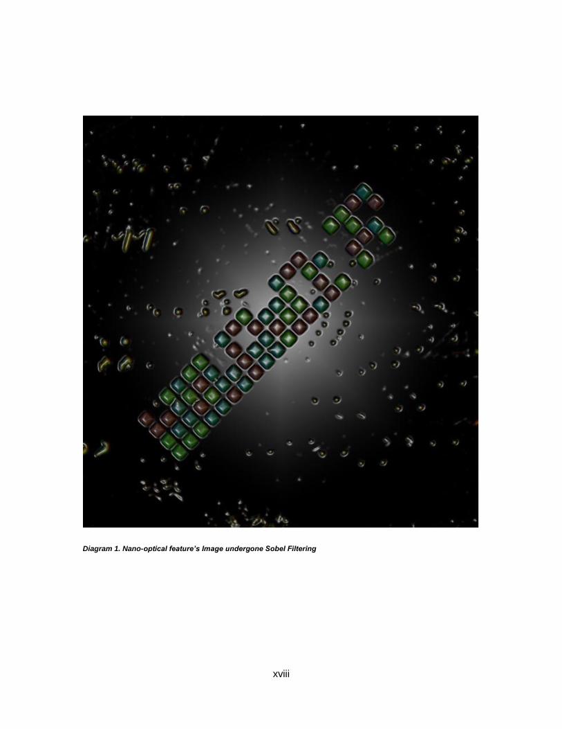
Introductory Image

Diagram 1. Nano-optical feature’s Image undergone Sobel Filtering

1

Chapter 1 Introduction

The use of different methods for encoding data has been researched by engineers and

computer scientists over the past decades. This work focuses on the benefits of using

alternative methods for encoding in order to achieve higher storage density and

transmission rates. The solution to high storage density and transmission in a system is

found through optimizing the data field structure and by using new physical media

(Nano-Structures) that can represent the data. The properties of the data field that can

be influenced by an alternate data structure are: i) the encoding scheme and ii) the

source entropy measurement. The properties of the media that can be influenced by an

alternate physical representation are: i) actual storage density and ii) storage

dimensions. We chose light and Nano-scale optical features as our data field and

medium respectively. Our research focuses on using Nano-optical features in the form of

periodic Nano-hole arrays for encoding data. The need for the development of a data

structure that encompasses and employs the unique properties of these features in data

storage and data transmission is also investigated. The plasmonic signature and the

diffracted spectrum of the Nano-hole arrays are regarded as a multidimensional field that

allows more data storage.

Based on the wavelength-dependent diffractive nature of the Nano-optical features, a

model is developed that allows defining a unit of information as an alternative to the

classical "bit". Easy to use signal acquisition techniques and the effects of Nano-scale

dimensions of the data storage media on the compression ratios are also part of this

work. Our preliminary results confirm that using Nano-optics for encoding increases the

accuracy for signal acquisition as a result higher signal to noise ratios for optical signals

can be achieved. Our encoding scheme allows for a numerical representable range for

unsigned integers of [0 255] in 4-bit (optical multi variation state bit) sequences. This is

equivalent to the numerical range of 8-bit long binary sequences.

2

The state of art encoding techniques used in different classes of authentication media

such as barcodes, radio frequency identification tags (RFIDs) and magnetic stripe cards

can contribute to both security via encrypting the data and data storage density through

introduction of materials and reading techniques by which the size of the stored data

variable decreases. Current technologies can be targeted by standard attack protocols

such as differential power analysis (DPA) and encoded media replication. Introduction of

the nano-optical features (NOF) through thesis referenced as [1] has proved to be

creating a secure medium for storing multi-color state optical variables as data color-bits.

The potential wavelength-dependent optically secure encoding medium sets the stage

for introduction of an encoding scheme that benefits from this multi-state variable signal

space and transforms different types of data into NOF-encoded media. This encoding

system aside from translating data from the digital format into optical nanostructures

must also compress the data in an efficient way to reduce the number of optical

nanostructures required to be fabricated for each data for the sake of system‟s cost

efficiency(fabrication of nanostructures is an expensive procedure). Some important

measure of using NOF in an encoding system is their ability to generate distinct colors in

their diffracted spectrum which can be used as multiple states of variation for a unit

information. Instead of having only two states of variation like binary integer based

variables, a NOF can have 3 or more depending on the ability of the reading optics to

resolve these colors in the reader‟s color-image. Through increasing the states of

variation of the encoding variable, the entropy of the encoded data is measured with a

smaller number and this lowers the number of code-words that source encoders such as

Huffman require to encode the entropy of a sequence of data [2]. The challenges for

manipulating the optical characteristics of the nano-optical features are both in physical

tune-up of the nano-scale diffractive structures and in the signal acquisition system.

Inherently, optical structures that produce a diffracted spectrum can be modelled as a

linear system. The equation that governs the system defines the position and degree of

diffraction of each wavelength based on the structure of the nano-optical system. Such

linearity however calls for a tune-up when the number of optical structures and

consequently the spatial dimension of the diffracted fields increase. In this thesis we

have addressed the problem of having numerous optical nanostructures being fabricated

in small distances with respect to one another and the appropriate tune-up of their

multiple diffracted spectra through solving the linear two variable equation of angular

3

dispersion for incidence wavelength and grating periodicity instead of its original form

which is a function of incidence angle and diffraction angle. The analysis allows for

rewriting the angular dispersion function for two independent variables (wavelength and

optical nanostructure periodicity) hence simulating the changes of diffracted wavelength

in different periodicity values. The second challenge for using optical nanostructures in

an encoding system is the signal acquisition and recognition. The diffracted spectrum of

the NOF produces a multi-colour image that for a contrasted background can be

extracted (data recovery) using standard image processing techniques. The scale of the

structures however when too small creates an aberration for the sensor. This aberration

can be defined as the mixing of diffracted colours in the sensor output. The degree of

difficulty of colour extraction depends on both the optical tune-up of the diffractive

nanostructures and the optics of the sensor. If the tune-up is considered optimal then

use of smaller scale nanostructures requires more advanced optics for the sensor. The

enhancement of the sensor‟s optics increases the price for a sensor design. We have

addressed this challenge in the thesis via use of standard two-dimensional histogram

analysis. The two-dimensional histogram based on a built-in MATLAB function known as

accumarray allows for construction of a multi-dimensional vector field in which each

colour value is first translated into CIE-LAB colour value and then become a vector with

three values (Hue, Chroma, Occurrence frequency). The technique we used in this work

needed to scale the LAB colour space values from their original [-128 128] range to a

more appropriate (unsigned integer) scale for further analysis. Our analysis has targeted

the extraction of each designated colour via referencing the simulated colour values

based to simulated colours predicted using diffraction equation. Use of a vector field

model referenced against a simulated (synthetic) colour map enables our algorithm to

extract the desired colour along with shades which are close to the designated colour in

Hue and Chroma value. Use of this method has eliminated the need for expensive optics

for detecting the colours that have been used in the nano-optical medium and enables

the decoding algorithm to detect colours using the readout signal of an off-the-shelf

inexpensive flatbed scanner. The minimum size nano-structures successfully detected

through the system were 20x20 square micron along with 20 micron distance in between

each two nanostructures. We have detected three colours (Red, Green and Blue) from

the aforementioned system.

4

The use of nanostructures and their diffracted spectrum as mentioned earlier in this

chapter gives rise to a multi-variation random variable model that instead of the

traditional bit (binary integer) system creating the base of current computation systems

can represent data with more than two states of variation. Each distinct colour in the

NOF can be regarded as a variation state and combination of these colours constructs a

multi-variation state encoding system that has a much larger numerical representation

range than the traditional bit. Aside from the numerical range in the case of a

transmission setup (Optical transmission and reception) the benefit of transmitting

variables with multiple variations states in oppose to only two the source encoder code-

words can measure the data entropy with a much smaller value hence reducing the

length of the code-words that are being transmitted. The aforementioned also enhances

the transmission rate via transmitting more data value through each transmitted optical

coloured signal. The inherent electromagnetic interference-resistance property of the

optical signals can also benefit the transmission setup as to the fact that higher signal to

noise ratios (SNR) can be achieved on the decoder side.

1.1. Synopsis

The state of the art information is presented in Chapter 2. The chapter will discuss the

fundamental concepts behind encoding scheme that have been employed on

Nanostructures introduced in [1]. It will briefly discuss the implementation of these

encoding schemes. With main focus on data-encoding, the chapter is dedicated to state

of the art schemes for digital data encoding using analog modulation and matching the

standard definitions with optical signals acquired from the diffracting spectrum of a

Nano-scale diffraction grating. Chapter 3 presents the design parameters of the interface

between digital data and Nano-optical features as means for encoding. The chapter also

presents system-level design of an encoder-decoder algorithm that accepts multi-format

data and channels it into the encoder using standard compressor algorithms. The effects

of the compressor algorithms have been discussed in detail. Further into the chapter

there are optical design parameters calculated for arbitrary optics systems in order to

design the Nano-optical features‟ periodicity. Chapter 4 presents the results and

discussion regarding the effects of employing the Nano-optical feature encoding to

5

encode data on storage density and the readout signal quality regarding the signal to

noise ratio of the acquired data.

1.2. Thesis Contribution

The main contributions to the project are the design and analysis of Nano-diffraction

grating system and its signal spectrum along with theoretical derivation of the incident

angles employed in the experimental parts. The design and implementation of system-

level algorithms to receive, channel, encode and decode the input data have been of the

specific contributions made in this thesis. The use of the standard compression

platforms in order to decrease the bulk input data and the encoder-decoder platform for

digital input to become optically stored have been the main focus of the contributions

made to the work. The results analysis is presented at the end of the chapter 4. Chapter

5 is dedicated to investigating the future potentials of using Nano-optical periodic

structures in data encoding and data transmission.

6

Chapter 2 Data Encoding

The state of the art data encoding techniques are categorized under two classes: 1)

Data encoding for transmission 2) Data encoding for storage. The objective of

techniques from both classes is modulation of a carrier in case of transmission encoding

and a translator in case of storage encoding. The objective of this thesis is to use

plasmonic structures fabricated in [1] for data storage. Hence the encoding for storage

will be discussed more in detail than encoding for transmission.

2.1. Data encoding for Transmission

In data encoding for transmission the encoder is a mathematical algorithm through which

the carrier which is a real-valued signal such as a wave is modulated. This modulation

changes properties such as amplitude or frequency of the carrier proportional to the

input binary data. For transmitting data such as images with numerical images greater

than 0 and 1, the encoder will first translate these numbers into the binary space and

after that it will modulate the carrier signal based on the variation of the binary signal.

Some examples of the state of the art encoding techniques used in data transmission

are as follows [3]:

1)-Digital data encoding using analog signals (Modems)

Encoding schemes that rely on analog signals to transform and transmit signals use a

carrier frequency. The data (binary or digital) is encoded through modulation of one of

the following three parameters of the carrier frequency: a)- Amplitude, b)- Fundamental

frequency and c)- Phase. Some schemes tend to combine these three in parts or in total

to achieve higher encoding rates. There are several methods in which an encoder can

manage to change the carrier frequency and enhance its bitrate and symbol rate (baud

rate) during the flow of digital data. Common examples of Digital-data vs. analog-

7

encoder are QPSK (Quadrature Phase-Shift Keying) encoding, QAM (Quadrature

Amplitude Keying) encoding, PSK (Phase-Shift Keying) encoding and DPKS (Differential

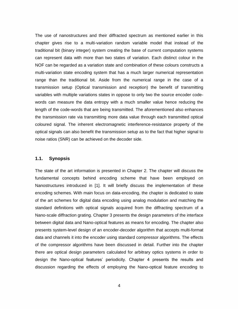
Phase-Shift Keying) encoding. In most of these encoding schemes a diagram is being

designed to map the streaming sequence of data into the mathematical (permutation)

space of the encoder. As a result the transmission line does not have to deal with the

data stream itself and hence error measurement algorithms can apply to the reception

setup prior to the decoder (Figure 2. 1).

Figure 2. 1 Standard modulation of carrier wave parameters

8

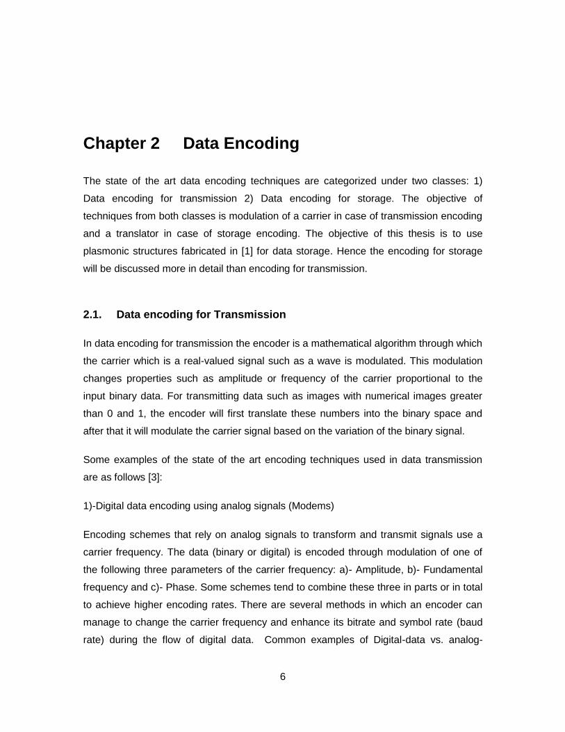
2)-Digital data encoding using digital signals (Wired LAN)

Digital signals unlike their analog counterparts are less prone to misinterpretation by the

decoder as to the fact that once achieved a certain threshold (e.g. Voltage) a digital

signal can maintain its amplitude based on hard thresholding of the decoder and

throughout the time it transmits within the channel. For an analog signal, every level of

the transmitted waveform is valid whereas for the digital signal, as long as being in a

certain range, only a few (two for binary encoding) levels are acceptable. An encoding

scheme using digital signals to encode has the following parameters [4]:

Bit-time: Time for a transmitter to generate the equivalent of one bit

Signal Recovery: Array of digital information that are outputted by the decoder

Signal Resolution: How well can the transmitted signals over a given bandwidth on a

certain channel.

The general scheme for such encoding setup is titles as line coding. In the line coding

scheme, binary information are presented in various serial signalling formats called line

codes. Graph below shows some popular line codes for digital encoding (Figure 2. 2):

Figure 2. 2 Basic functions of standard line coders

9

3)-Analog data encoding using digital signals

The significance of this encoding method is the oversampling capability. Analog signals

usually have limited frequency content which makes it easier to determine a minimum

Nyquist sampling rate for them in order to have them fully reconstructed during decoding

and demodulation. Generally speaking codecs can work both as means to convey

information and to store and encrypt data streams. Given the attenuation property of an

analog signal, use of digital signals to transmit and represent analog signals at discrete

levels, means less need for amplification (which tunes up the noise as well) and better

signal recovery for each bit of the digital representation. A codec as a result must

perform three tasks:

1) Analog Signal Sampling

2) Sampled Signal Quantization

3) Quantized Signal Encoding

Some standard codec examples are given in Table 1 :

Table 1 Examples of standard encodings used in analog encoding with digital signals

10

2.2. Definition of Data Field and Mathematical Definition of Data Encoding for Storage

Data is considered a field from which certain aspects or all of what exists in the field

needs to be encoded and stored. This field is known in communication and engineering

sciences as data field. Every system can have its own data field defined over a particular

set of mathematical quantifications. Similar to encoding for transmission, in order to

digitally store analog real valued data in a storage medium there has to be a signal

whose parameters undergo modulation. The encoder can perform this modulation as

part of a compression or expansion. The result of the modulation is a new sequence that

has one or more of its innate characteristics varying proportional to that of the original

(analog) data [5]. It is also necessary for the encoder to perform this modulation on a

certain arithmetic basis hence once digitally stored; the data can still undergo arithmetic

operation [6]. Similar to encoding for transmission, there should be a unit for storage.

This unit is called a unit information carrier or simply unit information. The computer

sciences model the unit information carrier as one bit which is also in a Boolean logic

framework. There are quantities of unit information carriers in a machine arithmetic

model where each transition between variables follows a true/false state and as a result

each function that receives and transmits a single state of true or false also is a Boolean

function. The Boolean algebra has full arithmetic space alongside a binary initial set. The

aforementioned property of Boolean algebra and Boolean functions makes its arithmetic

space (set of all bi-element sets and all functions operating on them) a suitable space for

storing information using only two elements of a given system [7]. Because a logic set

having only two distinct possibilities (e.g. true or false) is easy to replicate in a physical

sense (e.g. on/off, current/no current, voltage / no voltage) it seems intuitive for

modulating function to be a Boolean function [5]. For understanding the significance of

Boolean nature of the modulating function it is also necessary to understand the

representation of numbers in the set of data that is stored. Figure 2. 3 below show the

relationship between an original (analog) data set and the stored data set. The function

that maps in between the two sets is also the function that modulates the physical

parameters of a unit information carrier in order for it to be stored.

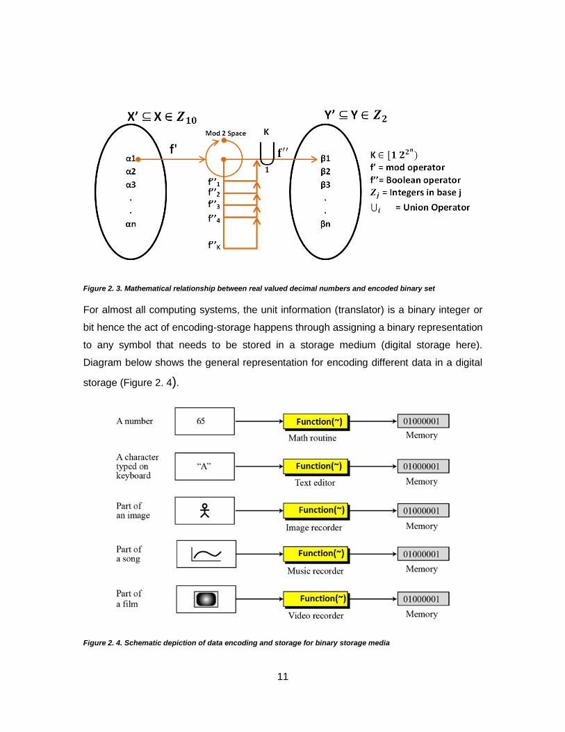
11

Figure 2. 3. Mathematical relationship between real valued decimal numbers and encoded binary set

For almost all computing systems, the unit information (translator) is a binary integer or

bit hence the act of encoding-storage happens through assigning a binary representation

to any symbol that needs to be stored in a storage medium (digital storage here).

Diagram below shows the general representation for encoding different data in a digital

storage (Figure 2. 4).

Figure 2. 4. Schematic depiction of data encoding and storage for binary storage media

12

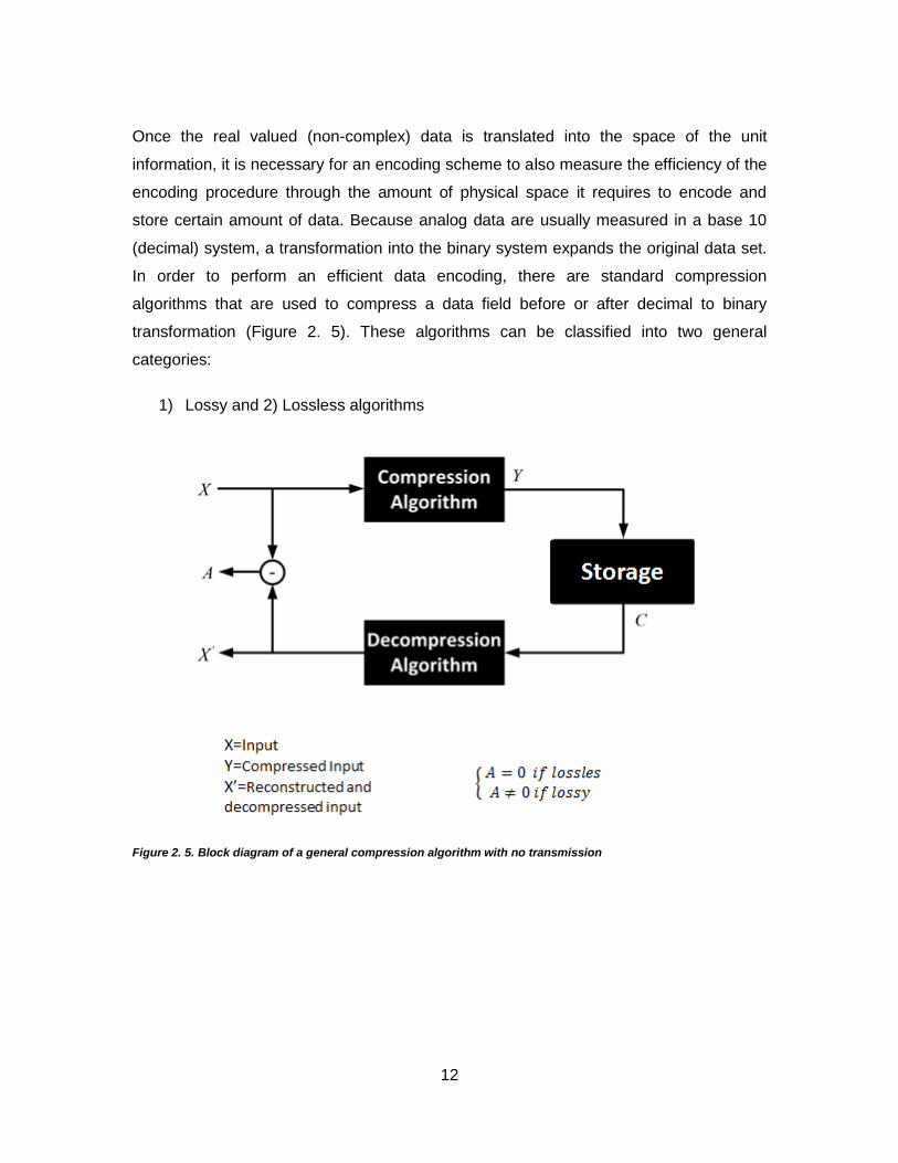
Once the real valued (non-complex) data is translated into the space of the unit

information, it is necessary for an encoding scheme to also measure the efficiency of the

encoding procedure through the amount of physical space it requires to encode and

store certain amount of data. Because analog data are usually measured in a base 10

(decimal) system, a transformation into the binary system expands the original data set.

In order to perform an efficient data encoding, there are standard compression

algorithms that are used to compress a data field before or after decimal to binary

transformation (Figure 2. 5). These algorithms can be classified into two general

categories:

1) Lossy and 2) Lossless algorithms

Figure 2. 5. Block diagram of a general compression algorithm with no transmission

13

Lossy Compression Algorithms

Some examples of most common lossy algorithms are given with brief descriptions

below:

1) Uniform Scalar Quantization:

Is the way of compressing distinct values outputted by a source through partitioning of

the input data range into intervals each being represented by a unique symbol or state.

Each quantizer can be uniquely described by its partition of the input range (encoder

side) and set of output values (decoder side). Quantization can be uniform. In a uniform

scalar quantization the inputs and output can be either scalar or vector. The quantizer

can partition the domain of input values into either equally spaced or unequally spaced

partitions. The end-points of partitions of equally spaced intervals in the input values of a

uniform scalar quantizer are called decision boundaries. The output value for each

interval is the midpoint of the interval and the length of each interval is called the step

size Δ [2] (Figure 2. 6).

Figure 2. 6. Uniform scalar quantizer basic function representation

14

Assuming that the input is uniformly distributed in the interval [-Xmax, Xmax] the rate of

the quantizer is R = ceil(log2 M). R is the number of bits needed to code the M output

values where the step size Δ is given by Δ = 2Xmax/M. For a uniform quantizer, the total

distortion (after normalizing) is twice the sum over the positive data:

2-1

2) Non Uniform Scalar Quantization

A uniform quantizer may be inefficient for an input source which is not uniformly

distributed hence the algorithm needs to use more decision levels where input is densely

distributed to lower distortion error and use fewer where data is sparsely distributed.

Total number of decision levels remains the same yet the quanitzer's output has less

distortion error for a given sample. Some common non uniform quantizer examples are:

1- Lloyd-Max quantization that iteratively estimates optimal boundaries based on

current estimates of reconstruction levels then updates the level and continues

until levels converge.

2- Companded quantization in which Input is mapped using a compressor function

G then quantized using a uniform quantizer. After transmission, quantized values

are mapped back using an expander function G-1.

3) Transform Coders

These algorithms transform the data through a transform matrix that translates data

values into a different mathematical space than that of the data. This new representation

of the data is then quantized using standard methods mentioned in the previous section

to compress the data. After quantization the transformed data will be recovered through

inverse transformation back into the original mathematical space it was taken from.

Examples of transform encoders are [8]:

15

1- Discrete Cosine Transform (DCT)

DCT is a widely used transform coding technique Spatial frequency indicates how many

times pixel values change across an image block The DCT formalizes this notion in

terms of how much the image contents change in correspondence to the number of

cycles of a cosine wave per block. The DCT decomposes the original signal into its DC

and AC components, following the techniques of Fourier analysis whereby any signal

can be described as a sum of multiple signals that are sine or cosine waveforms at

various amplitudes and frequencies. The inverse DCT (IDCT) reconstructs the original

signal. Its mathematical representation is as follows [2]:

2-2

Where N is the number of elements of the data file, x and y are spatial positions of a

data value (e.g. an image data), u,v are frequency components of the decomposed data

and α is an attenuation term to suppress the sequence expansion.

2- Wavelet Transform

A wavelet transform, similar to a Fourier Transform takes the image (or data) into the

frequency domain with the slight difference that what it outputs is localized both in

frequency and time due to an scaling factor that is calculated as a result of averaging the

16

entries in a particular window and a translation factor that is calculated due to altering

the length of the window that scans the signal. The combination of the two brings about

a collection of temporal frequency scattering of a signal in the wavelet space. The

resulting small functions that interact with each window (interval) of the signal are called

wavelets and they must have certain mathematical characteristics in order to be

invertible. Wavelet transform is described mathematically through [2]:

2-3

With the following condition for the frequency domain analysis:

2-4

Where γ(S,T) is the wavelet transform of the data, ψST is the wavelet notion and S, T are

Scaling and Translation of the signal. ψ(ω) is the Fourier transform of the wavelet and

must be zero at ω=0 for a fast decay of the wavelet approximating moments.

17

2.2.1. Lossless Compression Algorithms

During a lossless compression, the algorithm relies on three types of data redundancies

in order to perform compression. These redundancies due to the error free nature of the

algorithm cannot be eliminated or ignored hence the algorithm must take notes or pieces

of information (reconstruction clues) in order to further compress the code. Some of the

typical redundancies in a dataset used by lossless compression algorithms are: Coding

redundancy, Inter-pixel redundancy and Psycho-visual redundancy. Some standard

categories of lossless compression are [2]:

1) Variable-Length Encoding

Also referred to as source coding, this class of encoder reduces the bit or code length

redundancy in a set of data (or Image). The idea rises from the definition of entropy as

an average measure of uncertainty of occurrence of symbol (data value) within a data

field or from a data source. Each data field is usually described by the symbols that

represent information and a probability density vector that defines how often each

symbol is occurring in the field. By using the Shannon‟s entropy measure H(X), the class

of source variable length encoders assign variable lengths of binary code words to each

symbol on the data field in order to achieve an average less amount of total code length

in binary digits compared to a uniform assignment of code-words (Figure 2. 7).

Figure 2. 7. Probability of gray level occurrence of a stream of image data and the corresponding source entropy approximation (zero-order entropy) for source encoding

18

Of the existing algorithms, Huffman class is the optimum encoder for code word

redundancy reduction. The scheme in brief, pairs up the lowest probability symbols in

the source and assigns a single symbol to the pair as the rest of the source is being

coded. By sorting the probability of the new source (after pairing up all the lowest

probabilities in the sequence) the encoder produces a library entry and moves on to the

next cycle where it does the same to existing sequence. It can be shown that for a finite

length symbol source, the Shannon‟s entropy measure bounds the upper and lower

limits of an optimum code length as follows:

2-5

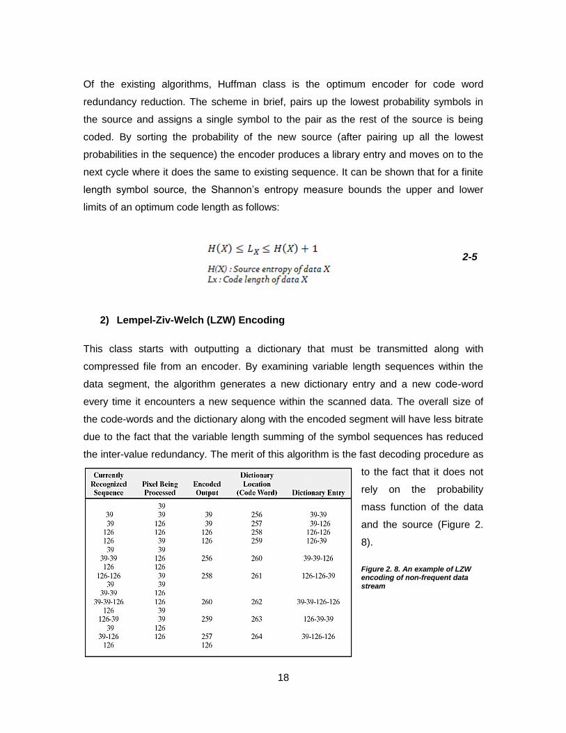
2) Lempel-Ziv-Welch (LZW) Encoding

This class starts with outputting a dictionary that must be transmitted along with

compressed file from an encoder. By examining variable length sequences within the

data segment, the algorithm generates a new dictionary entry and a new code-word

every time it encounters a new sequence within the scanned data. The overall size of

the code-words and the dictionary along with the encoded segment will have less bitrate

due to the fact that the variable length summing of the symbol sequences has reduced

the inter-value redundancy. The merit of this algorithm is the fast decoding procedure as

to the fact that it does not

rely on the probability

mass function of the data

and the source (Figure 2.

8).

Figure 2. 8. An example of LZW encoding of non-frequent data stream

19

2.3. State of the Art Data Encoding for Storage

The encoding for storage is performed in two different ways in standard methods: 1)-

Encoding for storage in computation devices (computers and microcontrollers) where the

data is stored either temporarily or permanently in the chip random memory and/or bios

unit. This encoding uses the potential difference between reference and a wire as an

indicator for existence of a binary one or zero. 2)-Encoding for storage in magnetic

storage media (analog media). In this storage scheme, the data are being represented

using the polarity of the magnetic field. In this method the encoder uses positive or

negative voltages to change the polarity of the magnetic particles in a magnetic particle

field. The decoder reads the data by detecting transition regions known as flux reversals

throughout the entire field which represent binary ones and non-transitioning areas

representing binary zeros. During this procedure, the encoder first acquires the raw

digital data and translates them into the domain of a wave. This wave is used to produce

change of polarities in the magnetic medium. For efficient encoding and decoding the

encoding scheme must have optimized parameters such as modulation order and

modulation parameter(s) that are being affected in the storage medium. Some most

practical and optimal encoding techniques for magnetic data storage are presented as

following [8][9]:

1)-Modified frequency modulation encoding

2)-Run-length-limited encoding

2.3.1. Modified Frequency Modulation Encoding

The modulation that separates the binary raw data and the magnetic particles in the

storage medium must determine the clocking of the input data. This means that the

decoder must know when the polarity changes represent a one and when represent a

zero. In this method the ones and zeros are represented with magnetic flux reversals

and clocking bits that separate the beginning of one bit from the end of the other. Figure

2. 9 shows how data current is being translated into the storage medium magnetic

polarisation.

20

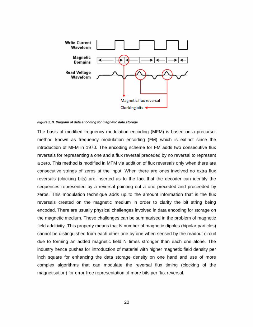
Figure 2. 9. Diagram of data encoding for magnetic data storage

The basis of modified frequency modulation encoding (MFM) is based on a precursor

method known as frequency modulation encoding (FM) which is extinct since the

introduction of MFM in 1970. The encoding scheme for FM adds two consecutive flux

reversals for representing a one and a flux reversal preceded by no reversal to represent

a zero. This method is modified in MFM via addition of flux reversals only when there are

consecutive strings of zeros at the input. When there are ones involved no extra flux

reversals (clocking bits) are inserted as to the fact that the decoder can identify the

sequences represented by a reversal pointing out a one preceded and proceeded by

zeros. This modulation technique adds up to the amount information that is the flux

reversals created on the magnetic medium in order to clarify the bit string being

encoded. There are usually physical challenges involved in data encoding for storage on

the magnetic medium. These challenges can be summarised in the problem of magnetic

field additivity. This property means that N number of magnetic dipoles (bipolar particles)

cannot be distinguished from each other one by one when sensed by the readout circuit

due to forming an added magnetic field N times stronger than each one alone. The

industry hence pushes for introduction of material with higher magnetic field density per

inch square for enhancing the data storage density on one hand and use of more

complex algorithms that can modulate the reversal flux timing (clocking of the

magnetisation) for error-free representation of more bits per flux reversal.

21

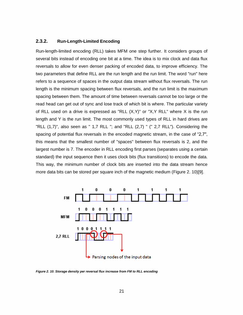
2.3.2. Run-Length-Limited Encoding

Run-length-limited encoding (RLL) takes MFM one step further. It considers groups of

several bits instead of encoding one bit at a time. The idea is to mix clock and data flux

reversals to allow for even denser packing of encoded data, to improve efficiency. The

two parameters that define RLL are the run length and the run limit. The word "run" here

refers to a sequence of spaces in the output data stream without flux reversals. The run

length is the minimum spacing between flux reversals, and the run limit is the maximum

spacing between them. The amount of time between reversals cannot be too large or the

read head can get out of sync and lose track of which bit is where. The particular variety

of RLL used on a drive is expressed as "RLL (X,Y)" or "X,Y RLL" where X is the run

length and Y is the run limit. The most commonly used types of RLL in hard drives are

"RLL (1,7)", also seen as " 1,7 RLL "; and "RLL (2,7) " (" 2,7 RLL"). Considering the

spacing of potential flux reversals in the encoded magnetic stream, in the case of “2,7",

this means that the smallest number of "spaces" between flux reversals is 2, and the

largest number is 7. The encoder in RLL encoding first parses (separates using a certain

standard) the input sequence then it uses clock bits (flux transitions) to encode the data.

This way, the minimum number of clock bits are inserted into the data stream hence

more data bits can be stored per square inch of the magnetic medium (Figure 2. 10)[9].

Figure 2. 10. Storage density per reversal flux increase from FM to RLL encoding

22

2.3.3. Optical Data Field and Current Optical Data Encoding for Storage

Current technology uses the digital domain parameters for both encoding and decoding

the analogue information into and from the optical media. The state of the art system can

be briefly described in the below graph (Figure 2. 11).

Figure 2. 11. Data encoding system with transmission properties (Optical Data Storage Ervin Meinders)

The optical data field can then be defined in two phases of the system; if the system

relies on grid writing and patterning then the data field is defined on the physical layer.

As a writer produces features such as grooves, rows or slits on the optical medium it

also, by leaving certain spaces between the grooves, induces sequences which form

tables and files that construct the data field [10][11]. One can distinguish between the

physical data field, which is a result of file production through a digital system prior to the

physical transfer onto the optical medium, and optical data field which is the total

perceivable luminance flux through the optical sensor. Although there is no profound

necessity for the two types of data field to be different from one another it appear so that

in some cases through different field descriptions one can achieve more efficient

compression and/or storage density. The recently employed concept of holography is an

example of having separated the electrical domain (digital) data field from the optical

data field (Figure 2. 12). In a holographic process the general idea is to not only record

the intensity changes of the incident light by means of the photosensitive material but

also to have the complete optical path of the incident light define that intensity

distribution. The equation of an incident electromagnetic wave is described through [12]:

23

2-6

It is the phase term that conveys information regarding the full path of the perceived

photon [13].

Figure 2. 12. An example of how the original (digital) and the successive optical data fields can differ; the fringe patterns of the interference create new data assortment hence a new field

24

2.4. Data Encoding for Storage in Authentication Industry

Authentication industry focuses on providing secure representation of personal or

commercial data for both individuals and organisations. The type of security is

dependent on the type of storage media and the capacity of information it possesses.

Large data capacity increases the authentication system‟s accuracy on one hand and

jeopardises the data security on the other. For large amount of personal data being

securely stored on an authentication device such as a card, the data must be encrypted

as well. It is also necessary implement types of media which resistant to external

disturbances such as electric or magnetic field or both (electromagnetic field) as well as

physical damages to the medium that can erase or corrupt the data. There have been

many generations of data authentication systems which use different encoding methods

to write and secure data. Some of these systems are simple and require no data

encryption (e.g. 1D, 2D and color barcodes) whereas some other have higher level of

security for protecting the data on the medium to be exposed to third party clients (e.g.

smart cards). The state of the art authentication media are discussed briefly in this

section.

2.4.1. Barcodes

This type of authentication media is a data entry streamline meaning that it shows a set

of data (alphanumeric data) in a particular direction. It has the advantage of being

printable on paper and easy to read via an optical reader setup. It also has lower levels

of error during detection due to its simple mechanism of encoding. Barcodes are

categorized based on the encoding dimensions. One dimensional barcodes offer length

dependent storage on only one direction or dimension. The 2D barcodes have

information recorded in more than one dimension (have data layout similar to a matrix).

The recently implemented color barcodes take advantage of presenting colors as an

extra encoding dimension as well. In general barcodes have following advantages and

disadvantages [14][15]:

Advantages: Easy to print, Not language dependent, Low error rate, Variety of print

methods, Full character set, Beam scannable

25

Disadvantages: Low capacity, Easy to acquire physical damage, Low data obscurity, No

encryption

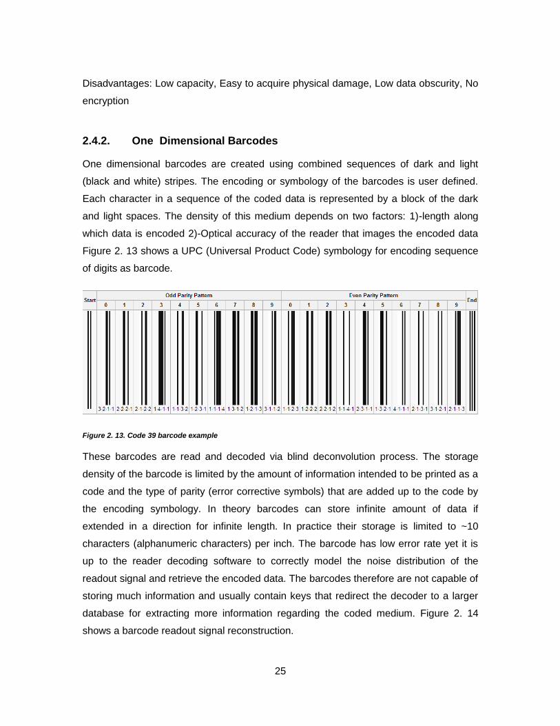
2.4.2. One Dimensional Barcodes

One dimensional barcodes are created using combined sequences of dark and light

(black and white) stripes. The encoding or symbology of the barcodes is user defined.

Each character in a sequence of the coded data is represented by a block of the dark

and light spaces. The density of this medium depends on two factors: 1)-length along

which data is encoded 2)-Optical accuracy of the reader that images the encoded data

Figure 2. 13 shows a UPC (Universal Product Code) symbology for encoding sequence

of digits as barcode.

Figure 2. 13. Code 39 barcode example

These barcodes are read and decoded via blind deconvolution process. The storage

density of the barcode is limited by the amount of information intended to be printed as a

code and the type of parity (error corrective symbols) that are added up to the code by

the encoding symbology. In theory barcodes can store infinite amount of data if

extended in a direction for infinite length. In practice their storage is limited to ~10

characters (alphanumeric characters) per inch. The barcode has low error rate yet it is

up to the reader decoding software to correctly model the noise distribution of the

readout signal and retrieve the encoded data. The barcodes therefore are not capable of

storing much information and usually contain keys that redirect the decoder to a larger

database for extracting more information regarding the coded medium. Figure 2. 14

shows a barcode readout signal reconstruction.

26

Figure 2. 14. Signal recovery process of a typical barcode decoding

2.4.3. Two-Dimensional Barcodes

Two dimensional barcodes are a second generation of barcode family with much larger

capacity compared to the one dimensional barcodes. These systems are also termed as

PDB (Portable Data Bases) due to larger data capacities they possess. Reading 2D

barcodes is done via image processing and contrast enhancement of the acquired

image from the encoded medium. 2D barcodes, similar to 1D barcodes are dependent

27

on how well the imaged encoded medium is resolved. The maximum data storage

capacity for some most common types are presented in Table 2.

Table 2 Common 2D barcode systems and their characteristics

With maximum storage of 32 KB, 2D barcodes can allow for up to 2Kb/in2 at 600 dpi

scan resolution (Compact Matrix Code aka CM Barcode).

2.4.4. Smart Cards

Another type of authentication with higher level of security and data capacity is the smart

card class. These media have more complex encoding and encryption implementation

compared to 1D and 2D barcodes. The security measures of smart cards are related to

both the type of data they carry, the amount of data on the card and decoding process.

Some common examples of smart cards are:

28

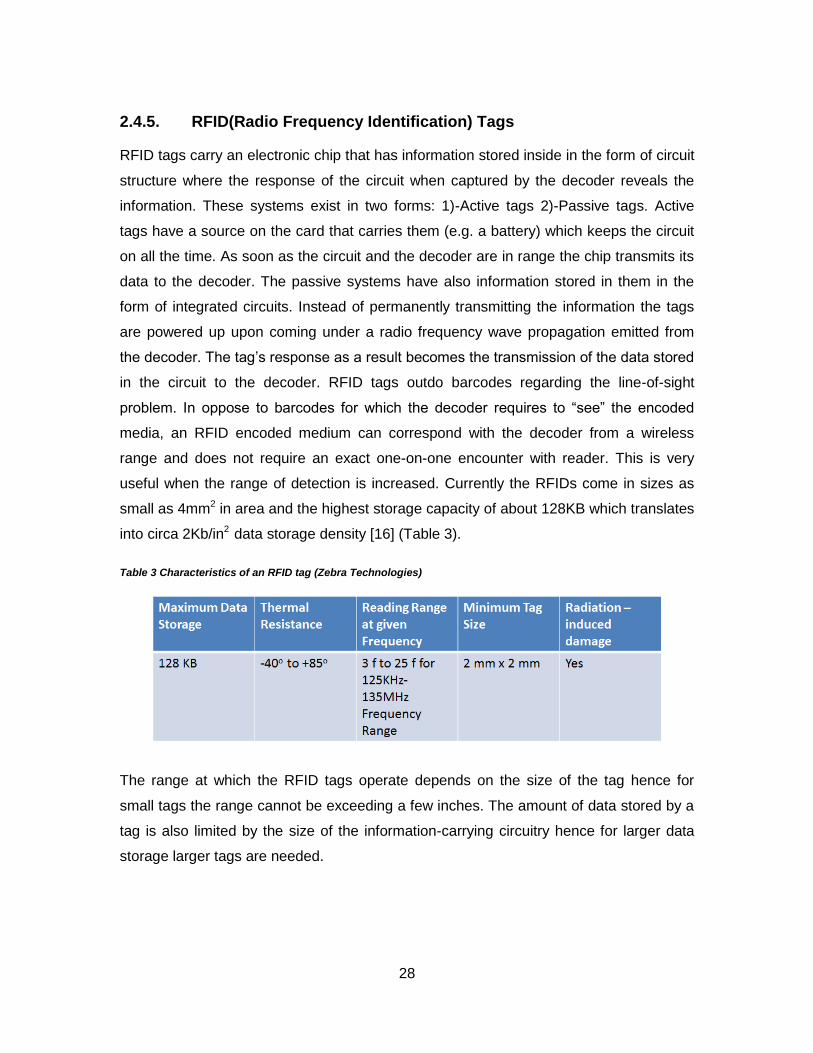
2.4.5. RFID(Radio Frequency Identification) Tags

RFID tags carry an electronic chip that has information stored inside in the form of circuit

structure where the response of the circuit when captured by the decoder reveals the

information. These systems exist in two forms: 1)-Active tags 2)-Passive tags. Active

tags have a source on the card that carries them (e.g. a battery) which keeps the circuit

on all the time. As soon as the circuit and the decoder are in range the chip transmits its

data to the decoder. The passive systems have also information stored in them in the

form of integrated circuits. Instead of permanently transmitting the information the tags

are powered up upon coming under a radio frequency wave propagation emitted from

the decoder. The tag‟s response as a result becomes the transmission of the data stored

in the circuit to the decoder. RFID tags outdo barcodes regarding the line-of-sight

problem. In oppose to barcodes for which the decoder requires to “see” the encoded

media, an RFID encoded medium can correspond with the decoder from a wireless

range and does not require an exact one-on-one encounter with reader. This is very

useful when the range of detection is increased. Currently the RFIDs come in sizes as

small as 4mm2 in area and the highest storage capacity of about 128KB which translates

into circa 2Kb/in2 data storage density [16] (Table 3).

Table 3 Characteristics of an RFID tag (Zebra Technologies)

The range at which the RFID tags operate depends on the size of the tag hence for

small tags the range cannot be exceeding a few inches. The amount of data stored by a

tag is also limited by the size of the information-carrying circuitry hence for larger data

storage larger tags are needed.

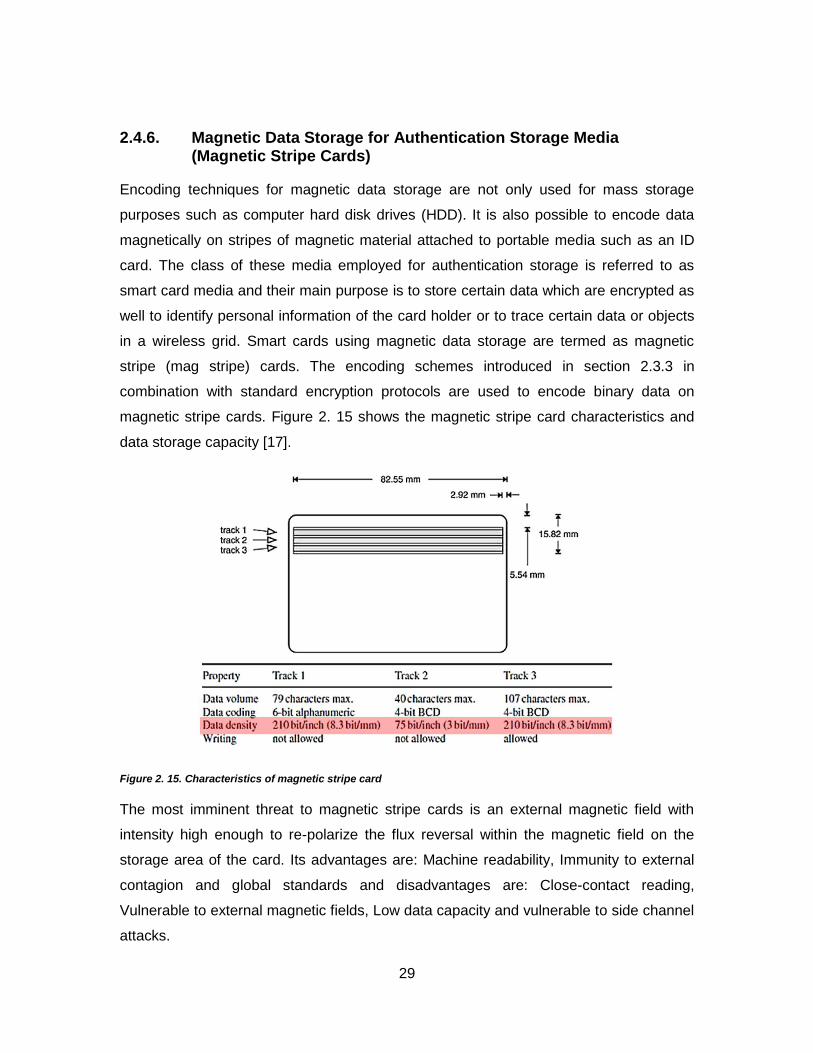
29

2.4.6. Magnetic Data Storage for Authentication Storage Media (Magnetic Stripe Cards)

Encoding techniques for magnetic data storage are not only used for mass storage

purposes such as computer hard disk drives (HDD). It is also possible to encode data

magnetically on stripes of magnetic material attached to portable media such as an ID

card. The class of these media employed for authentication storage is referred to as

smart card media and their main purpose is to store certain data which are encrypted as

well to identify personal information of the card holder or to trace certain data or objects

in a wireless grid. Smart cards using magnetic data storage are termed as magnetic

stripe (mag stripe) cards. The encoding schemes introduced in section 2.3.3 in

combination with standard encryption protocols are used to encode binary data on

magnetic stripe cards. Figure 2. 15 shows the magnetic stripe card characteristics and

data storage capacity [17].

Figure 2. 15. Characteristics of magnetic stripe card

The most imminent threat to magnetic stripe cards is an external magnetic field with

intensity high enough to re-polarize the flux reversal within the magnetic field on the

storage area of the card. Its advantages are: Machine readability, Immunity to external

contagion and global standards and disadvantages are: Close-contact reading,

Vulnerable to external magnetic fields, Low data capacity and vulnerable to side channel

attacks.

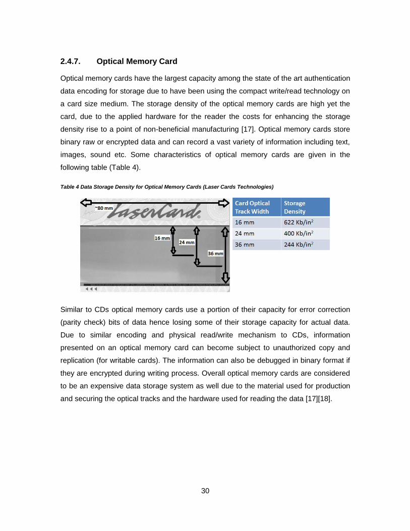
30

2.4.7. Optical Memory Card

Optical memory cards have the largest capacity among the state of the art authentication

data encoding for storage due to have been using the compact write/read technology on

a card size medium. The storage density of the optical memory cards are high yet the

card, due to the applied hardware for the reader the costs for enhancing the storage

density rise to a point of non-beneficial manufacturing [17]. Optical memory cards store

binary raw or encrypted data and can record a vast variety of information including text,

images, sound etc. Some characteristics of optical memory cards are given in the

following table (Table 4).

Table 4 Data Storage Density for Optical Memory Cards (Laser Cards Technologies)

Similar to CDs optical memory cards use a portion of their capacity for error correction

(parity check) bits of data hence losing some of their storage capacity for actual data.

Due to similar encoding and physical read/write mechanism to CDs, information

presented on an optical memory card can become subject to unauthorized copy and

replication (for writable cards). The information can also be debugged in binary format if

they are encrypted during writing process. Overall optical memory cards are considered

to be an expensive data storage system as well due to the material used for production

and securing the optical tracks and the hardware used for reading the data [17][18].

31

2.5. Project Motivation

The current encoding schemes for storage mentioned in 2.4, encounter some issues

regarding the storage density of the encoded medium as well as problems with respect

to a class of attacks called side channel attacks. Side-channel attacks use the electrical

signature (voltage or power) of the encoded medium to decrypt the data and to extract

the sequences that are being encoded. Low data storage density allows these attacks to

decrypt the secured combinations of data faster. Smart cards such as RFID tags and

magnetic stripe cards are vulnerable to these attacks. Another form of data extraction

from an encoded medium is use of exhausting search algorithms that can affect those

type of authentication media with low storage density. A third way to extract data from an

authenticated medium is to replicate the entire encoded medium onto another medium

and perform debugging analysis. Authentication media such as optical memory cards

which use CD-encoding technology can be decrypted this way.

Our intention through this work is to address these two issues (security and data storage

density) via use of plasmonic nanostructures. The thesis introduced in [1] has presented

plasmonic nanostructures which are capable of diffracting polychromatic (white) light in

different wavelengths (colors). It also presents a rather fast fabrication process for

fabricating the nanostructures using electron beam lithography (EBL). Following the

focus of [1] we intend to investigate the application of the presented structures to encode

data for storage purposes and measure the efficiency of an encoding system based on

these structures regarding the storage density and data security. Through our

simulation and experimental work we have proved that use of the plasmonic

nanostructures as means to store data is an efficient way for storing large amounts of

data in small spaces which are convenient for authentication media such as ID cards

and other similar documents. The state of the art authentication media such as

barcodes, RFID tags and optical memory cards all show deficiencies in either data

storage density or their security.

32

We have shown that the nanostructures can be tuned to reflect or transmit certain

wavelengths in a given direction and through combining them via a mathematical

algorithm hence they can be encoded in such way that their decryption becomes

extremely difficult and has high level of security. We also have shown that use of Nano-

scale structures allows for much higher data storage density than state of the art

authentication media. Our motivation is to design a system level implementation of the

mentioned Nano-optical structures in order to encode data on authentication media.

Through mathematical analysis via image processing techniques we have proven the

use of inexpensive reading setups can extract the encoded data in lower SNR (Signal to

Noise Ratio) and investigated the benefits of use of the mentioned plasmonic

nanostructures on Shannon‟s Typical Element Set (set of most probable outcomes for

an ergodic source of data) theoretically. Our motivation for the project is the employment

of a Nano-optical storage implementation for data encoding for storage in order to

enhance the security of the encoded data via removing the power analysis and side

channel attack possibilities. It also has been a focus of the work to introduce an

algorithm that receives and compresses data in an efficient way prior to preparing it for

nanofabrication on optical medium. The objectives for this thesis can be summarised as

follows:

1) Defining an appropriate encoding scheme for the Nano-optical structures

2) Defining an optical data-field using the diffracting spectrum of Nano-optical

structures

3) Investigating the performance of an optical encoder using periodic

nanostructures

4) Proof of concept for specific applications using the optically encoded data by

means of the periodic Nano-optical structures

2.5.1. Defining an Appropriate Encoding Scheme for Nano-Optical Structures

An encoding scheme enables the encoder using the nanostructures to be efficiently

employed in a way that during decoding the least amount of erroneous data is detected

33

by the decoder. Existence of multi-variable field parameters in optical media can

enhance the way data is being encoded and modulated in a way to achieve less error

rate during storage, transmission and less noise during recovery. In order to employ

these characteristics of an optical field, an encoding scheme needs to be designed to

incorporate the fixed or modulated variables related to the optical spectrum. In our case

the encoding scheme needs to address the optical characteristics of the Nano-optical

structures that we have intended to use in the experiment.

2.5.2. Defining an Optical Data Field using the Diffracted Spectrum of the Plasmonic Nanostructures

After designing the encoding scheme that will use the Nano-optical structures, we define

a field (data field) based on which the encoding scheme takes real-valued data as input

and transform these data into an arrangement of Nano-optical structures. The optical

data field consists of an optical unit information that is the smallest unit of optical

information that can be clearly represented by the optical medium and a modulation

parameter that is the characteristic of the optical spectrum undergoing change to

represent different information. By employing state of the art and novel Nano-fabrication

techniques, it has become possible to transfer designs for optical medium encoding onto

Nano-scale dimensions. This has become a motive for the project to design an optical

data field constructed onto Nano-optical structure media.

2.5.3. Investigating the Performance of an Optical Encoding Scheme using Periodic (and Plasmonic) Nano-Optical Structures

Depending on the wavelength of the incident light the distance traveled by the

wavelength without destructive attenuation is relatively much larger than an electrical

signal such as a voltage. It also requires less power to maintain the field amplitude of an

optical signal above degradation levels during signal transmission. These characteristics

allow for high performances during data recovery. This thesis has investigated the levels

of SNR at which full data recovery is possible over optical setups which have not been

compensated for optical aberration. This investigation measures the ability of the

designed encoding/decoding system using the full characteristics of the periodic optical

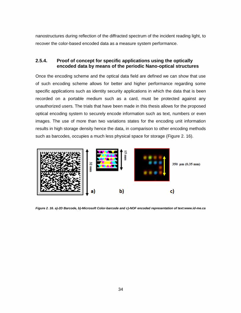
34

nanostructures during reflection of the diffracted spectrum of the incident reading light, to

recover the color-based encoded data as a measure system performance.

2.5.4. Proof of concept for specific applications using the optically encoded data by means of the periodic Nano-optical structures

Once the encoding scheme and the optical data field are defined we can show that use

of such encoding scheme allows for better and higher performance regarding some

specific applications such as identity security applications in which the data that is been

recorded on a portable medium such as a card, must be protected against any

unauthorized users. The trials that have been made in this thesis allows for the proposed

optical encoding system to securely encode information such as text, numbers or even

images. The use of more than two variations states for the encoding unit information

results in high storage density hence the data, in comparison to other encoding methods

such as barcodes, occupies a much less physical space for storage (Figure 2. 16).

Figure 2. 16. a)-2D Barcode, b)-Microsoft Color-barcode and c)-NOF encoded representation of text:www.id-me.ca

35

Chapter 3 Simulation and Theoretical Analysis

This chapter presents the analysis made in order to define the signal we use by

implementing a periodic nanostructures. Periodic nanostructures used in [1] act as

Nano-order diffraction gratings that can diffract an incident polychromatic (white) light in

different angularly separated directions. These diffracted spectra, if well resolved, can be

imaged by an imaging sensor such as a CCD (Charged Coupled Device) or CIS

(Contact Image Sensor) from distances far from the diffracting structures (in the

Fraunhofer optical domain). In order to calculate the correct tuning factor and resolve the

diffracted optical spectra in the sensor plane (image plane), we use MATLAB and linear

optics to calculate the optical paths which are going to emerge from the periodic

nanostructures both during transmission and reflection. The first step in our analysis is to

define the dimensions of the periodic optical nanostructures and the dimensions of the

signal received from them.

3.1. Defining the Physical Dimensions of the Periodic Optical Nanostructures and their Diffracted Spectrum

The periodic nanostructures under discussion act as diffraction gratings. The basic

function of a planar grating system is to create an angular dispersion in different orders

where the degree of dispersion of the light either transmitting or reflecting from the

grating has an inverse relationship with the groove density (periodicity) of the grating.

The term groove density is defined as number of holes, discontinuities or grooves in unit

measurement (length). In the case of a regular grating system the groove density or

groove frequency is defined as number of groove/mm whereas in the system under

discussion as to the fact that the unit measurement in use is nm hence the term groove

density is being defined as grooves /nm (Figure 3. 1) [19].

36

Figure 3. 1. Complete 3D diagram of a Nano-optical structure with in-plane incidence and diffraction

The procedure relies on defining a new storage system through introduction of a novel

implementation of Nano-scale diffraction grating structures that contributes to thorough

angular dispersion of a polychromatic incident light [19]. The data storage is a result of

the encoding of any numerical value that has been mapped into the permutation space

of these Nano-diffractive structures that will be referred to as Nano-Optical-Feature

(NOF) throughout the document. The permutation space will be the space of all possible

combinations of N number of NOF with varying array periodicities. The periodicity of a

NOF will be a parameter that influences the angular dispersion of the diffracted

wavelengths hence each NOF will diffract a specific wavelength at a specific degree of

alternation with respect to the grating normal in the Z direction. Such characteristic is the

foundation of this work in terms of choosing a certain angle (with respect to the grating‟s

normal) and define the type or state of variation of the NOF based on the wavelength

that is being diffracted in that particular direction There are the measures of separation

or dispersion path differences between each wavelength [19]. This term is related to the

dispersion power and resolving power of the grating. The resolving power of a grating is

its ability to unambiguously resolve or distinguish between two adjacent peaks with

similar amplitudes and different wavelengths. Theoretically the resolving power can be

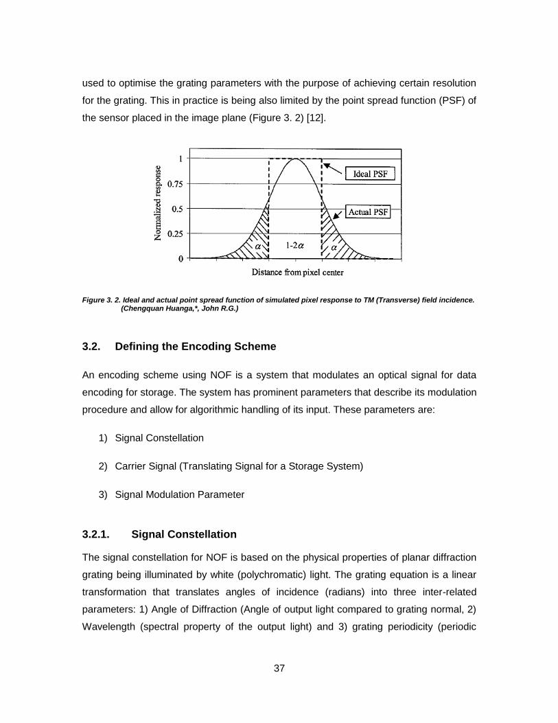
37

used to optimise the grating parameters with the purpose of achieving certain resolution

for the grating. This in practice is being also limited by the point spread function (PSF) of

the sensor placed in the image plane (Figure 3. 2) [12].

Figure 3. 2. Ideal and actual point spread function of simulated pixel response to TM (Transverse) field incidence. (Chengquan Huanga,*, John R.G.)

3.2. Defining the Encoding Scheme

An encoding scheme using NOF is a system that modulates an optical signal for data

encoding for storage. The system has prominent parameters that describe its modulation

procedure and allow for algorithmic handling of its input. These parameters are:

1) Signal Constellation

2) Carrier Signal (Translating Signal for a Storage System)

3) Signal Modulation Parameter

3.2.1. Signal Constellation

The signal constellation for NOF is based on the physical properties of planar diffraction

grating being illuminated by white (polychromatic) light. The grating equation is a linear

transformation that translates angles of incidence (radians) into three inter-related

parameters: 1) Angle of Diffraction (Angle of output light compared to grating normal, 2)

Wavelength (spectral property of the output light) and 3) grating periodicity (periodic

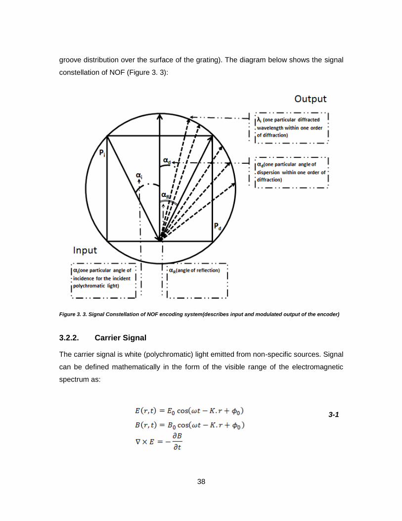
38

groove distribution over the surface of the grating). The diagram below shows the signal

constellation of NOF (Figure 3. 3):

Figure 3. 3. Signal Constellation of NOF encoding system(describes input and modulated output of the encoder)

3.2.2. Carrier Signal

The carrier signal is white (polychromatic) light emitted from non-specific sources. Signal

can be defined mathematically in the form of the visible range of the electromagnetic

spectrum as:

3-1

39

Where E is the electric field amplitude, B is the magnetic field amplitude, K=(kx,ky,kz) is

the spatial wave vector, r=(x,y,z), ω=2πf is the angular frequency and ϕ0 is the initial

phase in radians. The signal intensity is presented as [13]:

3-2

3.2.3. Modulation Parameters

Based on the signal constellation diagram and the signal mathematical description, what

undergoes a change as the carrier gets diffracted through the grooves of a diffraction

grating is dependent on which parameter of the grating equation is kept constant and

which is let to vary. For simplicity, we define the system to have fixed angle of reception

(hence the angle of diffraction is kept constant) and interpret the perceived signals as

being modulated by the angular frequency to produce variable colors or wavelengths as

interpreted by the spatial image sensor (Figure 3. 4). Transformation into signal domain

is defined as:

3-3

The order of the signal constellation depends on the number of available unit information

in the encoding scheme. As an example a binary system employs 8 single bits to

construct one byte and therefore the order of this constellation is 8. Some other example

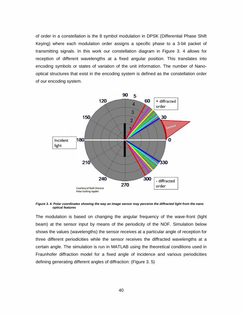
40

of order in a constellation is the 8 symbol modulation in DPSK (Differential Phase Shift

Keying) where each modulation order assigns a specific phase to a 3-bit packet of

transmitting signals. In this work our constellation diagram in Figure 3. 4 allows for

reception of different wavelengths at a fixed angular position. This translates into

encoding symbols or states of variation of the unit information. The number of Nano-

optical structures that exist in the encoding system is defined as the constellation order

of our encoding system.

Figure 3. 4. Polar coordinates showing the way an image sensor may perceive the diffracted light from the nano optical features

The modulation is based on changing the angular frequency of the wave-front (light

beam) at the sensor input by means of the periodicity of the NOF. Simulation below

shows the values (wavelengths) the sensor receives at a particular angle of reception for

three different periodicities while the sensor receives the diffracted wavelengths at a

certain angle. The simulation is run in MATLAB using the theoretical conditions used in

Fraunhofer diffraction model for a fixed angle of incidence and various periodicities

defining generating different angles of diffraction: (Figure 3. 5)

41

Figure 3. 5. a)-Green wavelength, b)-Blue Wave length and c)-Cyan color received by fixed angular position replace the initial signal (green) through change of grating periodicity

Table 5 shows the changes of the received wavelength for each periodicity at three

angles of diffraction. If a sensor is positioned at β1 angle, then the periodicities will be

defined as following as a function of received wavelengths:

3-4

42

Tracing the values of wavelengths received by sensor at angle β1 results in the

derivation of The modulating parameter from Eq(3-4) is the ratio m/K. (A=Integer)

Table 5 Variations of a Signal outcome based o figure. 41 simulations; The angles of diffraction vary with wavelength

3.3. Simulating the Conditions for Optimal Angular Dispersion

The property we use to tune our best imaging conditions (aside from choosing an

optimal optical solution for the imaging setup) is the Nano-optical structure‟s angular

dispersion. The matching of angular dispersion and the wavelength perceived by the

imaging sensor is the same for both slit-model-grating and the periodic Nano-optical

structures due to the existence of periodic discontinuity in the optical medium [19]

(Figure 3. 6).

43

Figure 3. 6. The illuminated length of a grating defines its resolved spectrum as a function of its periodicity

For a slit grating model in one dimension the resolving power can be defined as:

3-5

Without considerations for the imaging sensor and only based on the grating parameters

one can acquire the differential form of the grating equation presented in [19] as follows:

44

3-6

For acquiring Eq(3-6) the angle of incidence is being treated as a constant as to the fact

that the two angles of incidence and diffraction lie in a linear relationship. For acquiring

an optimizer parameter one can expand Eq(3-6) further into:

3-7

Using the identity:

3-8

And further into:

3-9

From Eq(3-9) we conclude that if the conditions for taking the derivative from the grating

equation is imposed (fixed angle of incidence), the optimizer for angular dispersion is the

grating frequency or reciprocal of the grating periodicity (Figure 3. 7).

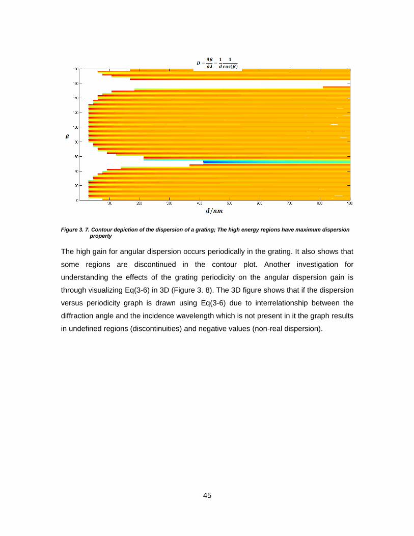
45

Figure 3. 7. Contour depiction of the dispersion of a grating; The high energy regions have maximum dispersion property

The high gain for angular dispersion occurs periodically in the grating. It also shows that

some regions are discontinued in the contour plot. Another investigation for

understanding the effects of the grating periodicity on the angular dispersion gain is

through visualizing Eq(3-6) in 3D (Figure 3. 8). The 3D figure shows that if the dispersion

versus periodicity graph is drawn using Eq(3-6) due to interrelationship between the

diffraction angle and the incidence wavelength which is not present in it the graph results

in undefined regions (discontinuities) and negative values (non-real dispersion).

46

Figure 3. 8. Three dimensional depiction of Fig (43). The negative values may correspond to complex results which have no measurable physical property

Graphs below show the computer simulation for an approximation based on Eq(3-9) for

different values for the fixed term sin (α).As Figure 3. 8 shows, the effects of the

changes of different angles of refraction on the dispersion is cyclic which corresponds to

the cyclic nature of the phase (and consequently the amplitude for a non-decaying

propagation) of the incident field. The overall transformations of the dispersion with

respect to both grating periodicity and diffraction angle can be shown through Figure 3.

9. As shown in Figure 3. 9, using Eq(3-9) corrects the relationship between the angular

dispersion and the incidence wavelength in oppose to what is resulted from Eq(3-6) in

Figure 3. 8. Further derivation results in an estimation of the way D or partial changes of

angular dispersion with respect to partial changes of wavelength, alters as a function of

grating periodicity and the incident wavelength. Eq(3-9) is a result of careful derivation

[19] with respect to changes of the wavelength. Through the latter procedure the angle

47

of incidence is treated as a constant, hence by using the alternate form of the dispersion

Eq(3-9) we can observe what are the effects of independent changes of the incident

wavelength on the angular dispersion (Figure 3. 9).

Figure 3. 9. a)- angular resolution for single angle of incidence b)-for multiple angles of incidence

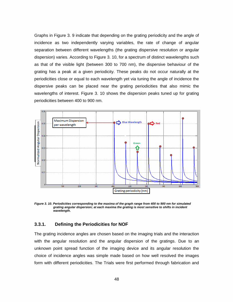
48

Graphs in Figure 3. 9 indicate that depending on the grating periodicity and the angle of

incidence as two independently varying variables, the rate of change of angular

separation between different wavelengths (the grating dispersive resolution or angular

dispersion) varies. According to Figure 3. 10, for a spectrum of distinct wavelengths such

as that of the visible light (between 300 to 700 nm), the dispersive behaviour of the

grating has a peak at a given periodicity. These peaks do not occur naturally at the

periodicities close or equal to each wavelength yet via tuning the angle of incidence the

dispersive peaks can be placed near the grating periodicities that also mimic the

wavelengths of interest. Figure 3. 10 shows the dispersion peaks tuned up for grating

periodicities between 400 to 900 nm.

Figure 3. 10. Periodicities corresponding to the maxima of the graph range from 400 to 900 nm for simulated grating angular dispersion; at each maxima the grating is most sensitive to shifts in incident wavelength.

3.3.1. Defining the Periodicities for NOF

The grating incidence angles are chosen based on the imaging trials and the interaction

with the angular resolution and the angular dispersion of the gratings. Due to an

unknown point spread function of the imaging device and its angular resolution the

choice of incidence angles was simple made based on how well resolved the images

form with different periodicities. The Trials were first performed through fabrication and

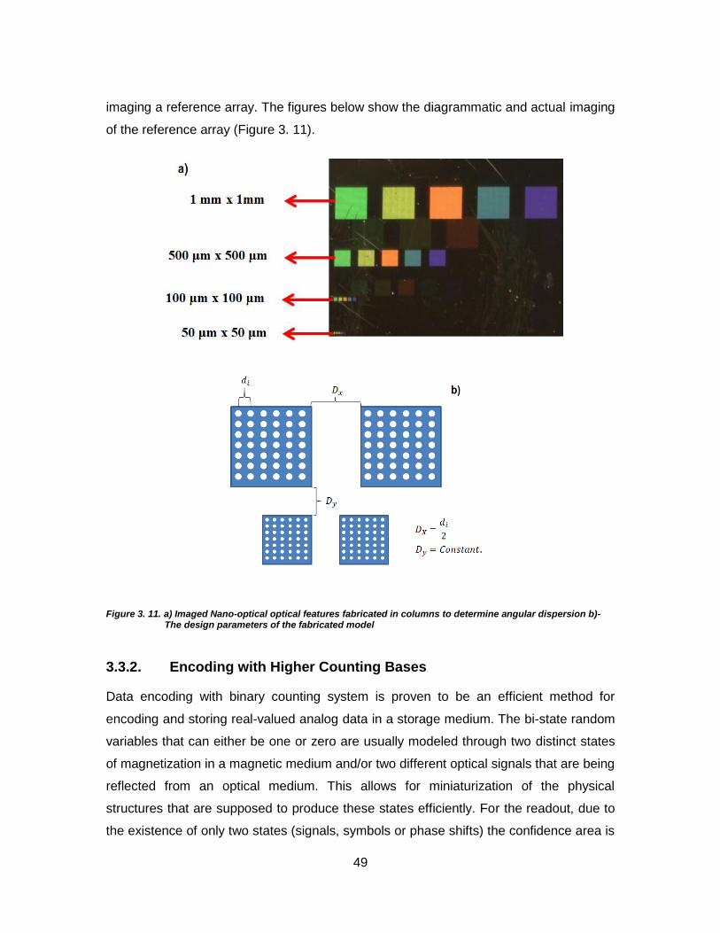
49

imaging a reference array. The figures below show the diagrammatic and actual imaging

of the reference array (Figure 3. 11).

Figure 3. 11. a) Imaged Nano-optical optical features fabricated in columns to determine angular dispersion b)-The design parameters of the fabricated model

3.3.2. Encoding with Higher Counting Bases

Data encoding with binary counting system is proven to be an efficient method for

encoding and storing real-valued analog data in a storage medium. The bi-state random

variables that can either be one or zero are usually modeled through two distinct states

of magnetization in a magnetic medium and/or two different optical signals that are being

reflected from an optical medium. This allows for miniaturization of the physical

structures that are supposed to produce these states efficiently. For the readout, due to

the existence of only two states (signals, symbols or phase shifts) the confidence area is

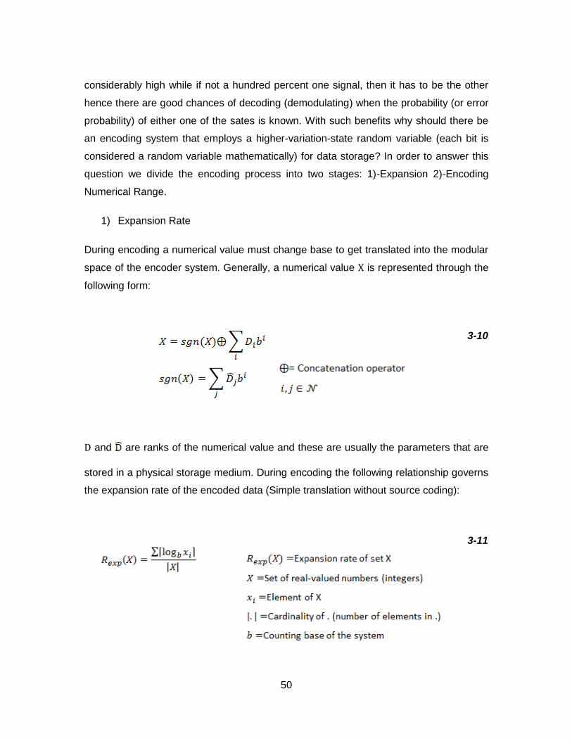
50

considerably high while if not a hundred percent one signal, then it has to be the other

hence there are good chances of decoding (demodulating) when the probability (or error

probability) of either one of the sates is known. With such benefits why should there be

an encoding system that employs a higher-variation-state random variable (each bit is

considered a random variable mathematically) for data storage? In order to answer this

question we divide the encoding process into two stages: 1)-Expansion 2)-Encoding

Numerical Range.

1) Expansion Rate

During encoding a numerical value must change base to get translated into the modular

space of the encoder system. Generally, a numerical value X is represented through the

following form:

3-10

D and are ranks of the numerical value and these are usually the parameters that are

stored in a physical storage medium. During encoding the following relationship governs

the expansion rate of the encoded data (Simple translation without source coding):

3-11

51

Adding to the states of variation of a unit information for storage via an encoding system

means less physical space needed to store the transformed data. There are boundaries

for how efficient the decrease will be as the number of variation states increases hence

one can decide first up to what extent is it efficient to increase the variation states of the

unit information carrier of the system second what is the cost of employment of more

physical aspects into a bit (Figure 3. 12). The figure shows the expansion rate of a linear

sequence of positive integers that has 1000 as its maximum value. The expansion rate

is calculated for b=[1,…,10]. The progression shows the rate of expansion for this

sequence for unit information that ranges from 1 to maximum 10 states of variation. The

solid lines show the rounded (upper boundary) values for the rate by which the

sequence is expanded.

Figure 3. 12. Data expansion rate bounded by upper and lower limits as a function of bit-variation states

This figure indicates that e.g. for a sequence of monotonically increasing numbers

(integers) with a maximum value of 1000, by encoding each element of the sequence

using a bit that has ten states of variation compared to a binary bit, the sequence

expands by a rate circa three times less hence the total number of unit information

needed to be stored for such sequence drops by a factor of three.

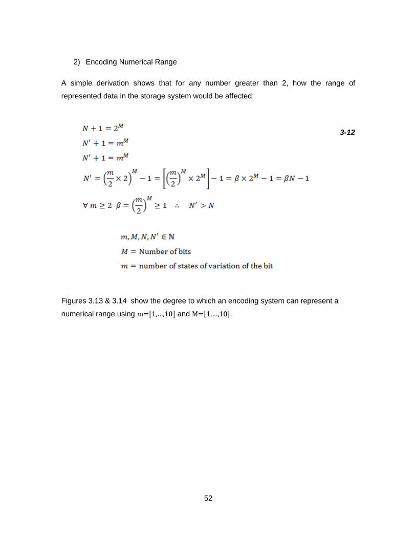
52

2) Encoding Numerical Range

A simple derivation shows that for any number greater than 2, how the range of

represented data in the storage system would be affected:

3-12

Figures 3.13 & 3.14 show the degree to which an encoding system can represent a

numerical range using m=[1,…,10] and M=[1,…,10].

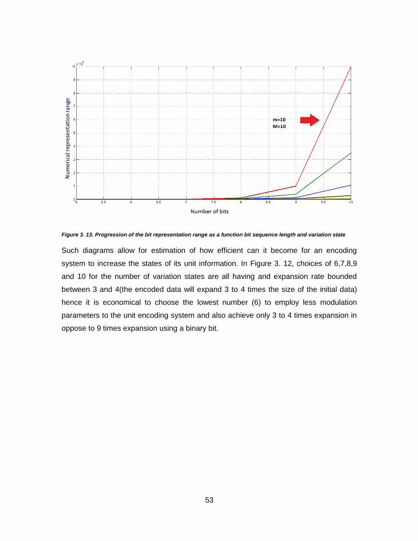
53

Figure 3. 13. Progression of the bit representation range as a function bit sequence length and variation state

Such diagrams allow for estimation of how efficient can it become for an encoding

system to increase the states of its unit information. In Figure 3. 12, choices of 6,7,8,9

and 10 for the number of variation states are all having and expansion rate bounded

between 3 and 4(the encoded data will expand 3 to 4 times the size of the initial data)

hence it is economical to choose the lowest number (6) to employ less modulation

parameters to the unit encoding system and also achieve only 3 to 4 times expansion in

oppose to 9 times expansion using a binary bit.

54

Figure 3. 14. Surface plot showing the peak numerical value representable by a 10-state bit string of length10

The result of Figure 3. 12 is that via choosing 4 or 5 states of variation the expansion

rate of a sequence of decimal integers from the range [0 1000] will drop from 9 times the

expansion down to ~4.5 times expansion. This decrease in the expansion rate is directly

proportional to the decrease in the amount of space which is required for encoding and

storing a given sequence of data. We choose 4 states of variation as a result of similar

expansion rate decrease between 4 states and 5 states of variation so that the encoding

bit will have 4 states: Sate “0”, Sate “1” , State “2” and State “3”. We match the simulated

periodicities from Figure 3. 10 to these states so that each state is represented by a

specific periodicity that mimics a particular wavelength (color). The four states chosen

for this work are then represented as: 1)-State “0” =no grating 2)-State “1”=450 nm

grating (Blue) 3)-State “2” =560 nm grating (Green) 4)-State”3”=650 nm grating (Red).

Applying these periodicities to Eq(3-4) allows for modulation of an integer value into a

combination of periodicities which will reflect their designated color, hence mapping from

integer values (digital values) into the analog domain of the diffracted spectrum of the

NOF.

55

The next step is to define an algorithm that receives data as an input and outputs the

encoded data using the NOF permutation space (combination of the four states of the

plasmonic nanostructures). The next section describes the designed algorithm part by

part and describes each block of the algorithm in detail.

3.4. System Level Implementation of the Nano-optical Encoder

The system level analysis focuses on an interface between an input (digital for this

matter) and an output that will be in the format of fabricated NOF as a result of the

aforementioned transformation in (Eq(3-4)). Because the interface requires a precise

element-wise modulation and due to cost and time boundaries of Nano-fabrication

procedures the first step in the interface is the implementation of an efficient

compression algorithm. Compression techniques have been reviewed in (2.3.2). Based

on the existing standards we choose to implement a combination of lossy and lossless

compressors to both decrease the bulk of the input data as much as possible while

maintaining a fair psycho-visual(human-based visual quality) fidelity criteria for the

reconstructed data after being read from the optically stored data. The scheme that has

been implemented is shown in the Figure 3. 15 below:

Figure 3. 15. Complete block diagram of NOF encoding system

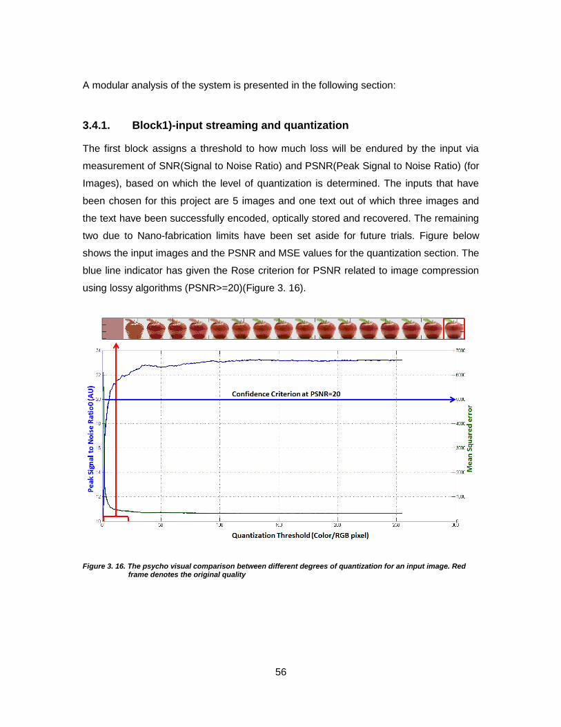
56

A modular analysis of the system is presented in the following section:

3.4.1. Block1)-input streaming and quantization

The first block assigns a threshold to how much loss will be endured by the input via

measurement of SNR(Signal to Noise Ratio) and PSNR(Peak Signal to Noise Ratio) (for

Images), based on which the level of quantization is determined. The inputs that have

been chosen for this project are 5 images and one text out of which three images and

the text have been successfully encoded, optically stored and recovered. The remaining

two due to Nano-fabrication limits have been set aside for future trials. Figure below

shows the input images and the PSNR and MSE values for the quantization section. The

blue line indicator has given the Rose criterion for PSNR related to image compression

using lossy algorithms (PSNR>=20)(Figure 3. 16).

Figure 3. 16. The psycho visual comparison between different degrees of quantization for an input image. Red frame denotes the original quality

57

The encoding of two larger images yields larger number of nano-optical elements

needed to be fabricated. Due to high hourly costs for both using the electron-beam

lithography machine and the developer material used to post-process the nano-optically

encoded data we resolved in encoding only three of the five initial images. In order to

demonstrate the performance of the encoder in compressing and encoding both the un-

fabricated images we present their equivalent compression ratios for three different

compression levels.

Figure 3. 17. a)-Different versions of cameraman image compressed by NOF encoder b)-PSNR for the encoded image using [1 255] colors per RGB pixel quantization.(The rest of the algorithm uses lossless encoding)

The number of optical arrays required for image „Cameraman‟ exceeds 5000. Although

as shown in Figure 3. 17 the compression ratio achieved by the algorithm is high yet

fabricating 5000 arrays for the sake of this thesis project is merely un-economical. Figure

on the next page shows similar information presented in Figure 3. 18, for image „Lena‟ :

58

Figure 3. 18 a)- Different versions of lena image compressed by NOF encoder b)-PSNR for the encoded image using [1 255] colors per RGB pixel quantization.(The rest of the algorithm uses lossless encoding)

The number of optically storable elements required to be fabricated for the image „lena‟

with results presented in Figure 3. 18 is circa 24000. This number is too large and cost

inefficient for fabrication during this master‟s thesis. The compression ratios presented

for these images on the other hand show more than 3 fold decrease in all the cases

presented in Figure 3. 17-18 and along with PSNR greater than 20 we conclude that the

perceptual quality of the two encoded and not fabricated images is acceptable for

encoding using our proposed encoder.

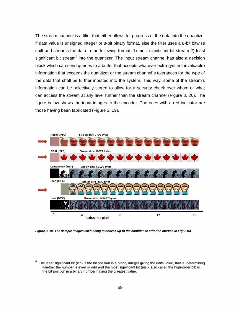
59

The stream channel is a filter that either allows for progress of the data into the quantizer

if data value is unsigned integer or 8-bit binary format, else the filter uses a 8-bit bitwise

shift and streams the data in the following format: 1)-most significant bit stream 2)-least

significant bit stream§ into the quantizer. The input stream channel has also a decision

block which can send queries to a buffer that accepts whatever extra (yet not invaluable)

information that exceeds the quantizer or the stream channel`s tolerances for the type of

the data that shall be further inputted into the system. This way, some of the stream‟s

information can be selectively stored to allow for a security check over whom or what

can access the stream at any level further than the stream channel (Figure 3. 20). The

figure below shows the input images to the encoder. The ones with a red indicator are

those having been fabricated (Figure 3. 19).

Figure 3. 19. The sample images each being quantized up to the confidence criterion marked in Fig(3.16)

§ The least significant bit (lsb) is the bit position in a binary integer giving the units value, that is, determining

whether the number is even or odd and the most significant bit (msb, also called the high-order bit) is the bit position in a binary number having the greatest value.

60

Figure 3. 20. Stream Channel Diagram; BITAND and BITSHIFT denote bitwise operation for maximum 8-bit value occurrence probability

3.4.2. Block2)-Run-Length Encoder and Source Encoder

The output of the quantizer passes through a two-phase run-length encoder in order to

decrease the bulk of the data before source encoding. Both the encoders in this block

are considered error free and/or lossless hence there is no measure of SNR or PSNR

defined for the data at this stage. The compression ratio however is considered. The

run-length encoder (RLE) performs a comparison between de-ranking the input values

into integer streams if the end result of an estimation is better, else it runs the data

through and streams the scanned data into the source encoder in the following format:

1)-unique set; these are the symbols that have been counted and stacked together, 2)-

counted set, these are the numbers for which each symbol has been repeated. The

graph shows the measure of RLE for a data stream after being compared through the

RLE and De-Rank & RLE block and the source encoder (Figure 3. 21).

61

Figure 3. 21. Run-Length Encoder Decision making Diagram

The source encoder receives the data from the RLE and based on whether or not the

user has defined a library entry chooses the encoder. In the case of library and also for

better compression the source encoder runs the data through a Huffman encoder and

then sends the decomposed and encrypted library to the storage (HDD), else the source

encoder chooses an arithmetic encoder that leaves no library behind and then sends the

encoded data to NOF permutation space transform block. In an extreme case, due to

having fabrication limits the three optically encoded images have been chosen to leave a

library behind. This way, the number of optical elements to be encoded on the optical

medium becomes quite limited and easy to handle during the fabrication process.

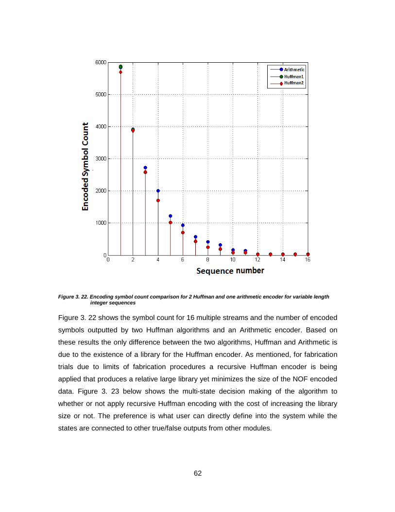
62

Figure 3. 22. Encoding symbol count comparison for 2 Huffman and one arithmetic encoder for variable length integer sequences

Figure 3. 22 shows the symbol count for 16 multiple streams and the number of encoded

symbols outputted by two Huffman algorithms and an Arithmetic encoder. Based on

these results the only difference between the two algorithms, Huffman and Arithmetic is

due to the existence of a library for the Huffman encoder. As mentioned, for fabrication

trials due to limits of fabrication procedures a recursive Huffman encoder is being

applied that produces a relative large library yet minimizes the size of the NOF encoded

data. Figure 3. 23 below shows the multi-state decision making of the algorithm to

whether or not apply recursive Huffman encoding with the cost of increasing the library

size or not. The preference is what user can directly define into the system while the

states are connected to other true/false outputs from other modules.

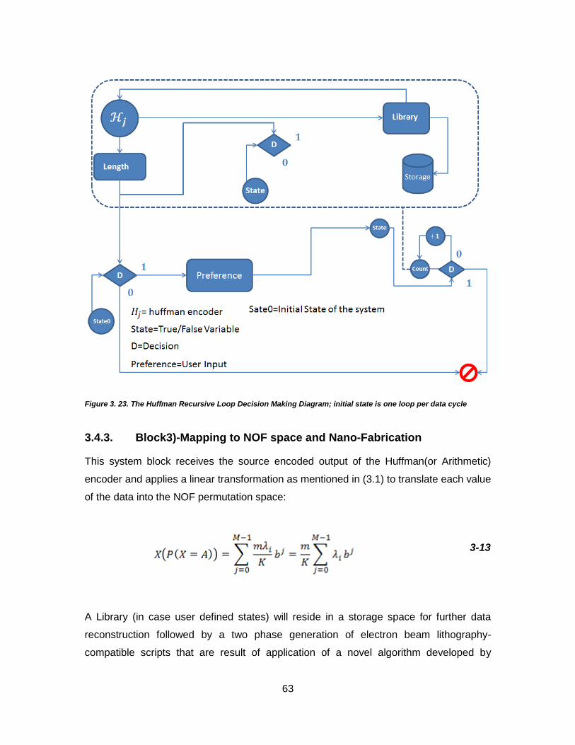
63

Figure 3. 23. The Huffman Recursive Loop Decision Making Diagram; initial state is one loop per data cycle

3.4.3. Block3)-Mapping to NOF space and Nano-Fabrication

This system block receives the source encoded output of the Huffman(or Arithmetic)

encoder and applies a linear transformation as mentioned in (3.1) to translate each value

of the data into the NOF permutation space:

3-13

A Library (in case user defined states) will reside in a storage space for further data

reconstruction followed by a two phase generation of electron beam lithography-

compatible scripts that are result of application of a novel algorithm developed by

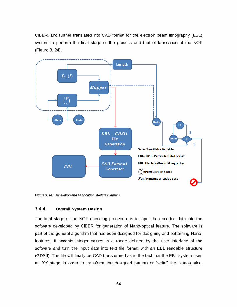
64

CiBER, and further translated into CAD format for the electron beam lithography (EBL)

system to perform the final stage of the process and that of fabrication of the NOF

(Figure 3. 24).

Figure 3. 24. Translation and Fabrication Module Diagram

3.4.4. Overall System Design

The final stage of the NOF encoding procedure is to input the encoded data into the

software developed by CiBER for generation of Nano-optical feature. The software is

part of the general algorithm that has been designed for designing and patterning Nano-

features, it accepts integer values in a range defined by the user interface of the

software and turn the input data into text file format with an EBL readable structure

(GDSII). The file will finally be CAD transformed as to the fact that the EBL system uses

an XY stage in order to transform the designed pattern or “write” the Nano-optical

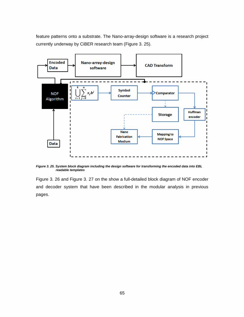
65

feature patterns onto a substrate. The Nano-array-design software is a research project

currently underway by CiBER research team (Figure 3. 25).

Figure 3. 25. System block diagram including the design software for transforming the encoded data into EBL readable templates

Figure 3. 26 and Figure 3. 27 on the show a full-detailed block diagram of NOF encoder

and decoder system that have been described in the modular analysis in previous

pages.

66

Figure 3. 26. NOF Encoder block diagram

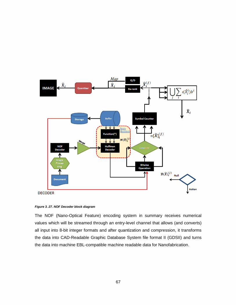
67

Figure 3. 27. NOF Decoder block diagram

The NOF (Nano-Optical Feature) encoding system in summary receives numerical

values which will be streamed through an entry-level channel that allows (and converts)

all input into 8-bit integer formats and after quantization and compression, it transforms

the data into CAD-Readable Graphic Database System file format II (GDSII) and turns

the data into machine EBL-compatible machine readable data for Nanofabrication.

68

Chapter 4 Experimental Results and Discussion

The experimental setup for encoding data has been the electron beam lithography(EBL)

setup at 4D-Labs located in Simon Fraser University‟s Physics department (Figure 4. 1)

and the trials have been three color images of various sizes and the text (www.ID-

ME.ca) all encoded using the NOF encoder algorithm. As mentioned earlier due to

minimization of the optical nanostructures that were needed to be fabricated on the

optical medium for encoding, the algorithm chose to perform the source coding using

Huffman coding with 5 repetition loop to decrease the size of the data encoded on

through EBL leaving libraries that were stored in a buffer (HDD or other storage media)

for data reconstruction.

Figure 4. 1. The EBL setup at 4D labs located in Simon Fraser’s Physics Department

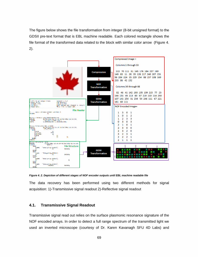
69

The figure below shows the file transformation from integer (8-bit unsigned format) to the

GDSII pre-text format that is EBL machine readable. Each colored rectangle shows the

file format of the transformed data related to the block with similar color arrow (Figure 4.

2).

Figure 4. 2. Depiction of different stages of NOF encoder outputs until EBL machine readable file

The data recovery has been performed using two different methods for signal

acquisition: 1)-Transmissive signal readout 2)-Reflective signal readout

4.1. Transmissive Signal Readout

Transmissive signal read out relies on the surface plasmonic resonance signature of the

NOF encoded arrays. In order to detect a full range spectrum of the transmitted light we

used an inverted microscope (courtesy of Dr. Karen Kavanagh SFU 4D Labs) and

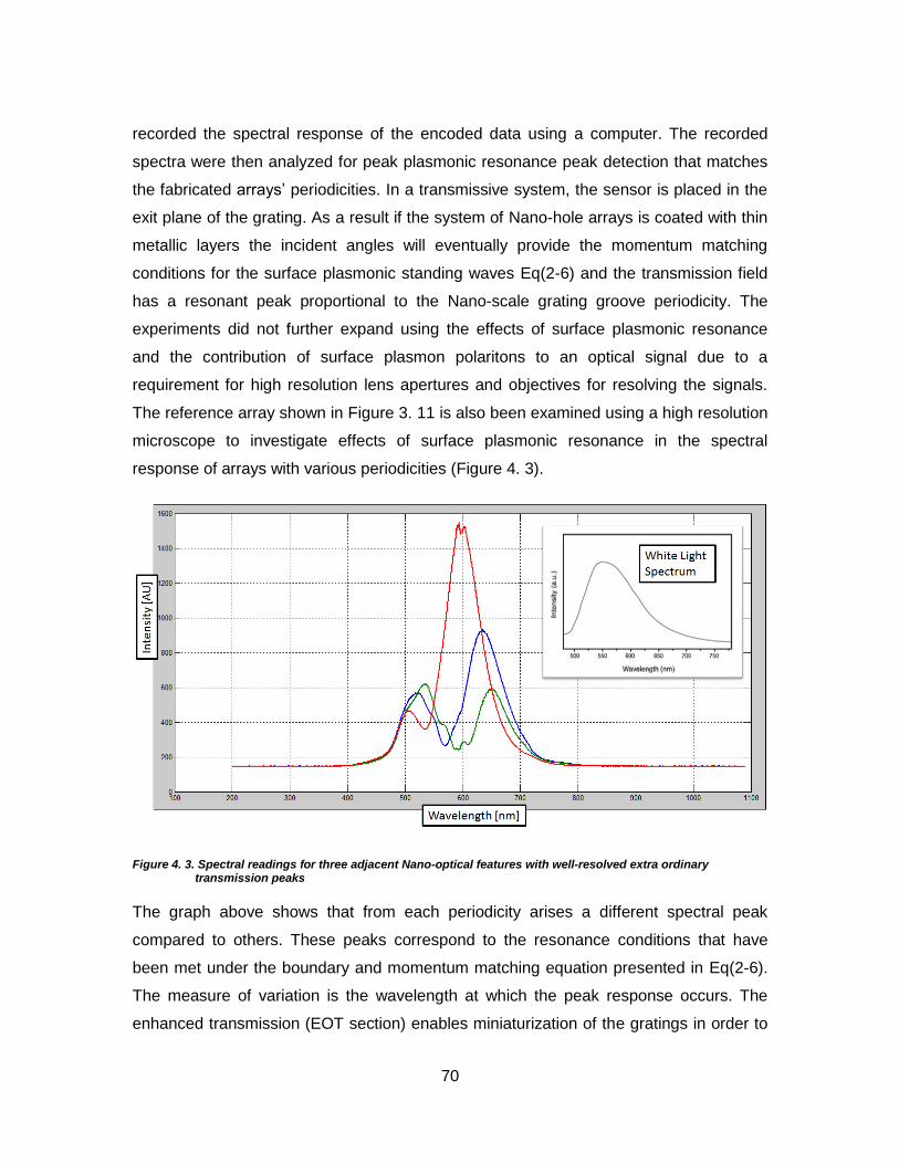
70

recorded the spectral response of the encoded data using a computer. The recorded

spectra were then analyzed for peak plasmonic resonance peak detection that matches

the fabricated arrays‟ periodicities. In a transmissive system, the sensor is placed in the

exit plane of the grating. As a result if the system of Nano-hole arrays is coated with thin

metallic layers the incident angles will eventually provide the momentum matching

conditions for the surface plasmonic standing waves Eq(2-6) and the transmission field

has a resonant peak proportional to the Nano-scale grating groove periodicity. The

experiments did not further expand using the effects of surface plasmonic resonance

and the contribution of surface plasmon polaritons to an optical signal due to a

requirement for high resolution lens apertures and objectives for resolving the signals.

The reference array shown in Figure 3. 11 is also been examined using a high resolution

microscope to investigate effects of surface plasmonic resonance in the spectral

response of arrays with various periodicities (Figure 4. 3).

Figure 4. 3. Spectral readings for three adjacent Nano-optical features with well-resolved extra ordinary transmission peaks

The graph above shows that from each periodicity arises a different spectral peak

compared to others. These peaks correspond to the resonance conditions that have

been met under the boundary and momentum matching equation presented in Eq(2-6).

The measure of variation is the wavelength at which the peak response occurs. The

enhanced transmission (EOT section) enables miniaturization of the gratings in order to

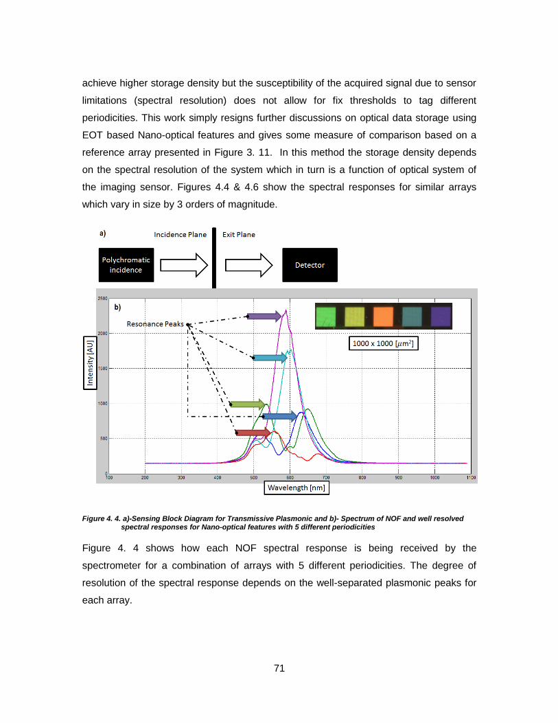
71

achieve higher storage density but the susceptibility of the acquired signal due to sensor

limitations (spectral resolution) does not allow for fix thresholds to tag different

periodicities. This work simply resigns further discussions on optical data storage using

EOT based Nano-optical features and gives some measure of comparison based on a

reference array presented in Figure 3. 11. In this method the storage density depends

on the spectral resolution of the system which in turn is a function of optical system of

the imaging sensor. Figures 4.4 & 4.6 show the spectral responses for similar arrays

which vary in size by 3 orders of magnitude.

Figure 4. 4. a)-Sensing Block Diagram for Transmissive Plasmonic and b)- Spectrum of NOF and well resolved spectral responses for Nano-optical features with 5 different periodicities

Figure 4. 4 shows how each NOF spectral response is being received by the

spectrometer for a combination of arrays with 5 different periodicities. The degree of

resolution of the spectral response depends on the well-separated plasmonic peaks for

each array.

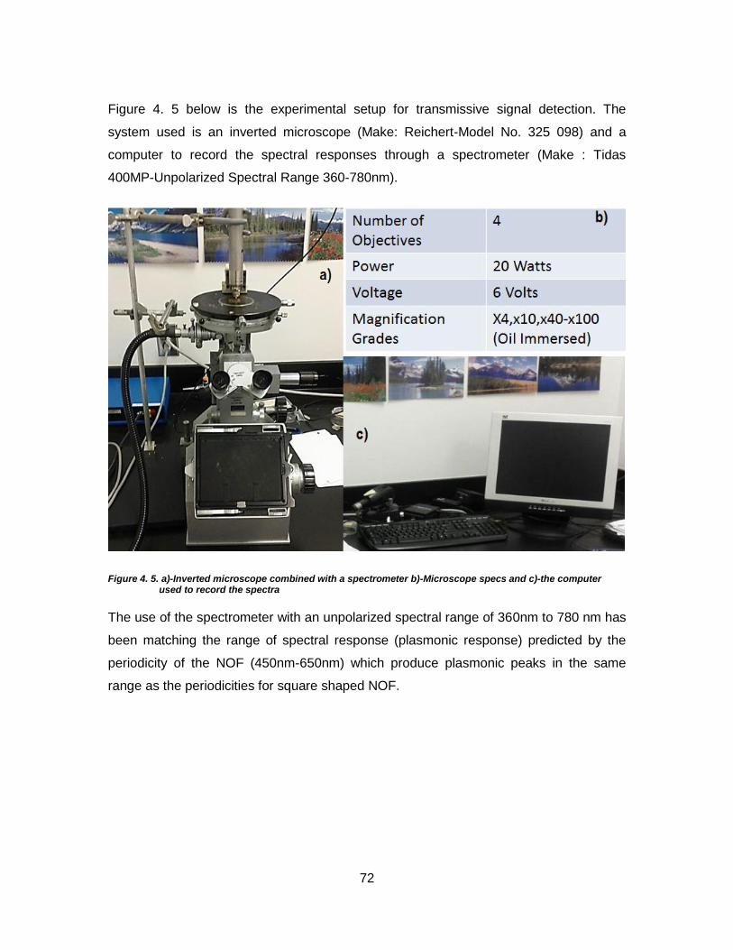
72

Figure 4. 5 below is the experimental setup for transmissive signal detection. The

system used is an inverted microscope (Make: Reichert-Model No. 325 098) and a

computer to record the spectral responses through a spectrometer (Make : Tidas

400MP-Unpolarized Spectral Range 360-780nm).

Figure 4. 5. a)-Inverted microscope combined with a spectrometer b)-Microscope specs and c)-the computer used to record the spectra

The use of the spectrometer with an unpolarized spectral range of 360nm to 780 nm has

been matching the range of spectral response (plasmonic response) predicted by the

periodicity of the NOF (450nm-650nm) which produce plasmonic peaks in the same

range as the periodicities for square shaped NOF.

73

Figure 4. 6. Unresolved spectral responses for Nano-optical features with 5 different periodicities

The transform that takes the real-valued quantities into the signal domain for

transmissive signal is defined as the overall (sum or integral) of the propagations of

periodic structure being illuminated as a function of its reciprocal lattice vectors Gx, Gy.

For a square array as one used in Figure 3. 11 the reciprocal lattice vectors are the

same, hence the resonant wavelength as a function of the grating periodicity is

calculated through the following equations Figure 4. 7 [20][21]:

4-1

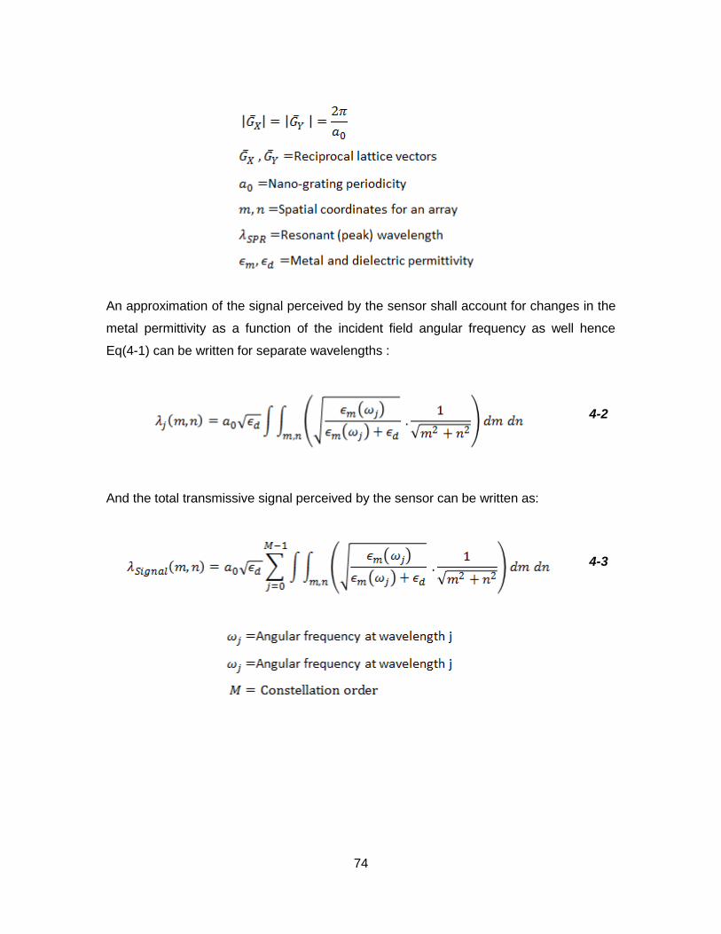
74

An approximation of the signal perceived by the sensor shall account for changes in the

metal permittivity as a function of the incident field angular frequency as well hence

Eq(4-1) can be written for separate wavelengths :

4-2

And the total transmissive signal perceived by the sensor can be written as:

4-3

75

Figure 4. 7 shows the spatial distribution of resonance peaks as orthogonal lattice

directions m and n.

Figure 4. 7. Position and direction of the resonance peaks in a square lattice

The signal collection direction means to have a sensor recording the spectral responses

of the NOF in either m or n direction which construct an orthogonal (perpendicular)

coordinate system as shown in Figure 4. 7 .

4.2. Reflective Signal Acquisition

A reflective signal is acquired as collection of the diffracted orders. Depending on the

periodicity and what has been discussed in (3.2) these responses were captured via

scanning the arrays with a flat-board scanner setup with maximum resolution of 9600

dpi. Scanners use a cylindrical lens to collect the back-reflected light from the scanning

object while a light source (usually a polychromatic source) at an angle is incident on the

scanning object. The back reflected light is gathered at an angle normal (or other) to the

scanner‟s bed. For a diffraction grating under the scan, this collection angle translates

into a grating-periodicity-dependent diffraction angle for the fixed angle of incidence and

hence what received by the scanner image sensor (CCD or CIS) is the result of pixel by

pixel collection of particular wavelengths (colors) to form an image.

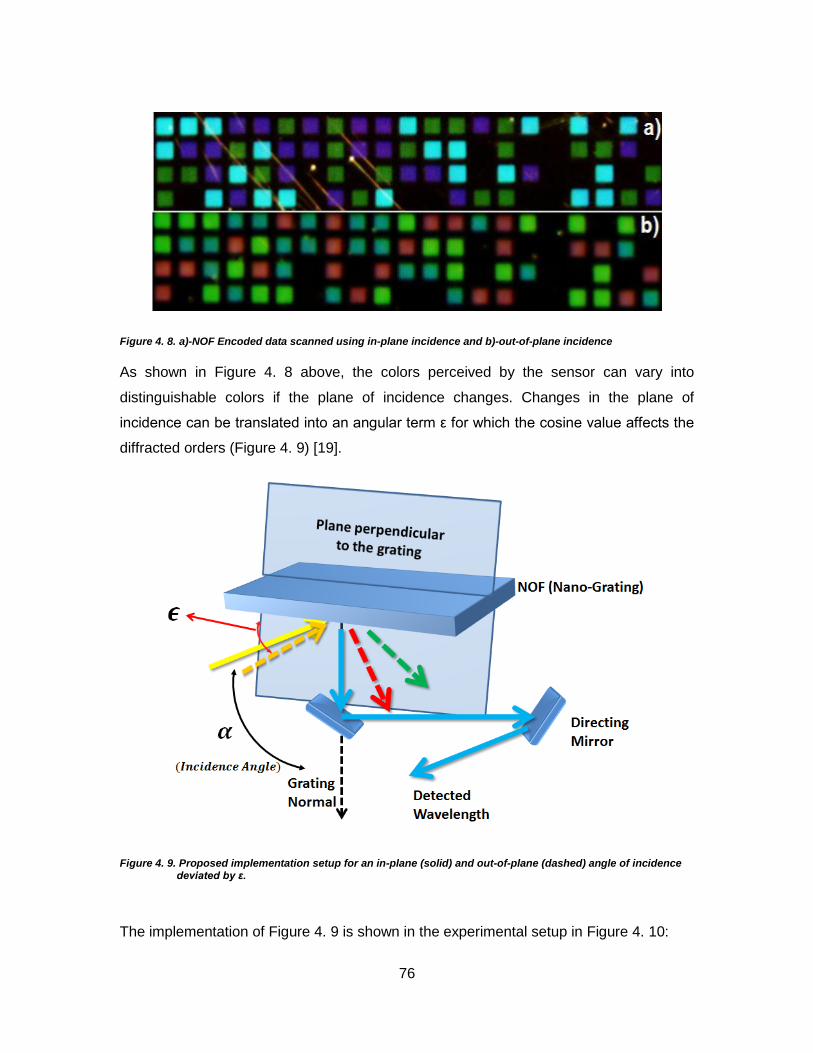
76

Figure 4. 8. a)-NOF Encoded data scanned using in-plane incidence and b)-out-of-plane incidence

As shown in Figure 4. 8 above, the colors perceived by the sensor can vary into

distinguishable colors if the plane of incidence changes. Changes in the plane of

incidence can be translated into an angular term ε for which the cosine value affects the

diffracted orders (Figure 4. 9) [19].

Figure 4. 9. Proposed implementation setup for an in-plane (solid) and out-of-plane (dashed) angle of incidence deviated by ε.

The implementation of Figure 4. 9 is shown in the experimental setup in Figure 4. 10:

77

Figure 4. 10. Implementation of out-of-plane incidence (canonical diffraction) for NOF using flat-board scanner

The storage density of the stored data was measured over the recovery of the stored

data from the largest sample (Tagged as “Joee”) encoded via 200 x 200 um arrays down

to the smallest sample(Tagged as “CFLG”) stored with 50 x 50 um arrays of Nano-

optical features. The signal acquisition is shown in Figure 4. 11 & 12.

Figure 4. 11. The sensing setup for the reflective diffracting spectrum of the NOF. The inclined angle of sensing can be translated into errors for the calculated angle of incidence for clarity and error correction

78

Figure 4. 12. NOF in reflective sensing setup and during diffraction. The temporal scan interval is being ignored in spectral calculations

The storage density of a reflected signal (excluding the effects of EOT and surface

plasmonic resonance in the acquired signal) is a result of diffracting light under a certain

angle. The acquired image can then be investigated with respect to how well each Nano-

optical feature can be separated from an adjacent one or how well the boundaries in the

color space can be resolved. Figures below show the storage density achieved through

down scaling the Nano-optical feature sizes over the encoding process.

79

Figure 4. 13. a)-Acquired storage density with large 200x200μm2 arrays b)-18-folds increase in the storage density

via encoding with 20x20 μm2 arrays

The storage densities presented in Figure 4. 1 can vary if the inter-array distance

increases or decreases.

4.2.1. Encoded Data Reconstruction

After producing a readout signal for the Nano-optical feature based encoded data, image

processing techniques were implied to achieve a separated color image from the

acquired image. As a result of the color segmentation, the encoded matrix is recovered

and the data can be fed into the main compressor platform of the algorithm in reverse

order to be regenerated. In brief the recovery procedure can be summarized in:

80

Figure 4. 14. Visualisation of the data recovery using a)grid scanning b)numeral evaluation c)Huffman decode d)reverse comparison e) reverse symbol counter (from left to right)

This part of the project can be a stand-alone module that could be either receiving

feedback from the main algorithm regarding how to reconstruct data in case of a library

that decrypts the optical data or simply perform reading and extraction of the numerical

data that has been outputted by the compression algorithm (Figure 4. 14).

The procedure for data recovery is divided into the following steps:

a) Image Dimension Approximation

The image from the sensor is in the TIFF format hence the first step for data recovery is

to perform a color segmentation process in order to extract the dominant colors in the

medium. The steps to do so are as following:

1- Using the fabrication and scan coordinates of the substrate isolating the encoded

area(Figure 4. 15-4.16):

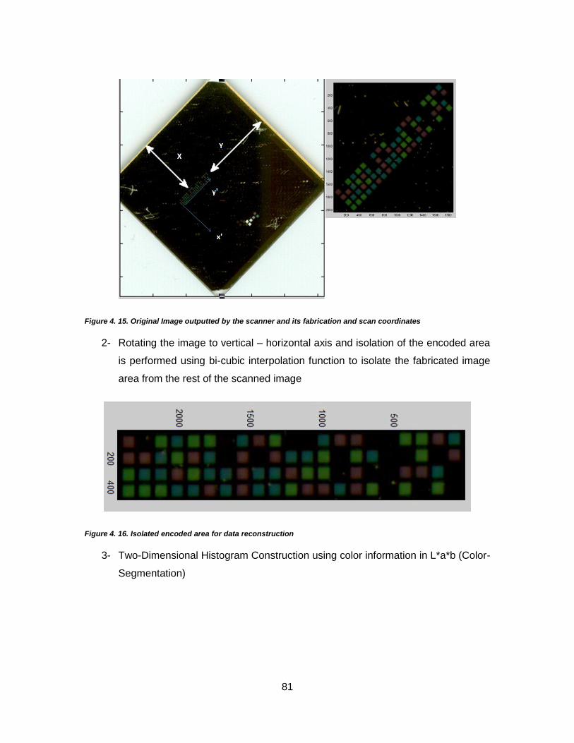
81

Figure 4. 15. Original Image outputted by the scanner and its fabrication and scan coordinates

2- Rotating the image to vertical – horizontal axis and isolation of the encoded area

is performed using bi-cubic interpolation function to isolate the fabricated image

area from the rest of the scanned image

Figure 4. 16. Isolated encoded area for data reconstruction

3- Two-Dimensional Histogram Construction using color information in L*a*b (Color-

Segmentation)

82

Figure 4. 17. Hue-Vs. Chroma information accumulated to form orthogonal 2D space. Each point in this space corresponds to a spatial distribution of colors

Through definition of a 2D histogram and due to the angularly well-resolved and well-

dispersed diffracted spectrum by the NOF, this information is found to be spatially

scattered across the 2D space of the Histogram in Figure 4. 17. In a 2D histogram the

number of points in the Hue-Chroma Space(2D distribution of image color information) is

tuneable hence a visually user-defined parameter can be set to monitor the distribution

of the color information and decide for more or less points included in the histogram

(histogram bins). In case of occurrence of undesirable effects such as mixed points that

represent more than one color group, spatial filters such as averaging or blind

deconvolution was performed to create stronger contrast and amplify the edges of the

acquired image [22][23] (Figure 4. 18).

83

Figure 4. 18. a)-Effect of noise on the color extraction (segmentation) procedure; b)-use of averaging filter and a blind deconvolution for edge preservation sets the color data more visibly apart for extraction

84

4- Extraction of Isolated Color-Channels using acquired color-masks from 2):(Figure

4. 19)

Figure 4. 19. The image being decomposed to its major color-content using mask-multiplication

The next step after the color-isolation is to merge the isolated single-valued images to

form a tri-color sample (Figure 4. 20):

Figure 4. 20. Three dimensional concatenation of the single color images

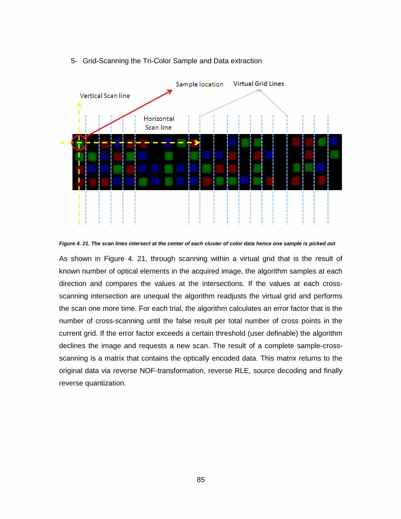
85

5- Grid-Scanning the Tri-Color Sample and Data extraction

Figure 4. 21. The scan lines intersect at the center of each cluster of color data hence one sample is picked out

As shown in Figure 4. 21, through scanning within a virtual grid that is the result of

known number of optical elements in the acquired image, the algorithm samples at each

direction and compares the values at the intersections. If the values at each cross-

scanning intersection are unequal the algorithm readjusts the virtual grid and performs

the scan one more time. For each trial, the algorithm calculates an error factor that is the

number of cross-scanning until the false result per total number of cross points in the

current grid. If the error factor exceeds a certain threshold (user definable) the algorithm

declines the image and requests a new scan. The result of a complete sample-cross-

scanning is a matrix that contains the optically encoded data. This matrix returns to the

original data via reverse NOF-transformation, reverse RLE, source decoding and finally

reverse quantization.

86

4.2.2. Encoded Results

An overall 4 trials were successfully made in order to optically modulate and encode

data in the form Nano-optical features with varying periodicity and in the form of arrays

of periodic Nano-structures. Throughout this chapter the results of optical encoding are

presented and results are being compared to some commercially available data storage

media for finite-length, low-cost, high-security data storage. The results are presented in

the following table (Table 6):

Table 6 Images stored using recursive source encoding within NOF algorithm along with their space on optical material and library size on disk

The large compression ratios are the consequence of recursive Huffman loop on the

encoded data, hence storage of relatively large libraries. These trials have been all

targeting an economical fabrication of the NOF and not an efficient data storage capacity

for the compressed data libraries. It can be deducted through the results of this work that

through increasing the modulation order of the input data (adding more colors to the

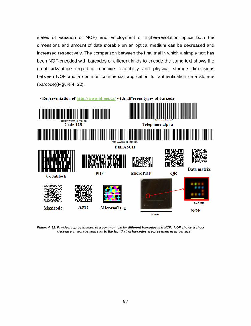
87

states of variation of NOF) and employment of higher-resolution optics both the

dimensions and amount of data storable on an optical medium can be decreased and

increased respectively. The comparison between the final trial in which a simple text has

been NOF-encoded with barcodes of different kinds to encode the same text shows the

great advantage regarding machine readability and physical storage dimensions

between NOF and a common commercial application for authentication data storage

(barcode)(Figure 4. 22).

Figure 4. 22. Physical representation of a common text by different barcodes and NOF. NOF shows a sheer decrease in storage space as to the fact that all barcodes are presented in actual size

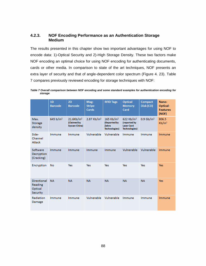
88

4.2.3. NOF Encoding Performance as an Authentication Storage Medium

The results presented in this chapter show two important advantages for using NOF to

encode data: 1)-Optical Security and 2)-High Storage Density. These two factors make

NOF encoding an optimal choice for using NOF encoding for authenticating documents,

cards or other media. In comparison to state of the art techniques, NOF presents an

extra layer of security and that of angle-dependent color spectrum (Figure 4. 23). Table

7 compares previously reviewed encoding for storage techniques with NOF:

Table 7 Overall comparison between NOF encoding and some standard examples for authentication encoding for storage

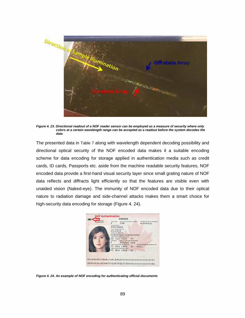
89

Figure 4. 23. Directional readout of a NOF reader sensor can be employed as a measure of security where only colors at a certain wavelength range can be accepted as a readout before the system decodes the data

The presented data in Table 7 along with wavelength dependent decoding possibility and

directional optical security of the NOF encoded data makes it a suitable encoding

scheme for data encoding for storage applied in authentication media such as credit

cards, ID cards, Passports etc. aside from the machine readable security features, NOF

encoded data provide a first-hand visual security layer since small grating nature of NOF

data reflects and diffracts light efficiently so that the features are visible even with

unaided vision (Naked-eye). The immunity of NOF encoded data due to their optical

nature to radiation damage and side-channel attacks makes them a smart choice for

high-security data encoding for storage (Figure 4. 24).

Figure 4. 24. An example of NOF encoding for authenticating official documents

90

In contrast to barcodes that require an encoding symbology for decoding information,

NOF has a numerical range that accepts almost any input and allows for large

encryption possibilities using combinations of different characters or letters and numbers

(Figure 4. 25).

Figure 4. 25. Mathematical quantifications of a security check system parameters to produce encodable data

4.2.4. Comparison between NOF and recently reported Nano-Optical Multi-State Data Encoding Systems

There has been various reports on use of Nano-optical structures and particularly those

range below the diffraction limits for an optical reader (half of the wavelength with high-

end optics) to encode multi-variation state bits. These reports usually target those media

which are capable of withholding changes made to them through an illumination of a

polychromatic or monochromatic beam. These media can also contain additional

degrees of storage that can be affected via modulating other beam parameters such as

phase, polarization and etc. In trials presented in [24], the encoding system has

91

employed a five-variation-state-bit (penta-bit) in order to encode distinguishable

information by use of mono-chromatic incidence beam (Nd:YAG Laser with wavelength

of 532 nm) as writing means and azo-polymer (azo-moiety Disperse Red-1) blended into

poly-methylmethacrylate (PMMA) with a 25% molar concentration as the optical

medium. Both encoding and decoding processes are done via NSOM (Near-Field

Scanning Optical Microscopy) and the Table 8 shows the parameters of the encoded

data using this report. The encoded bits show variation states as changes made to the

voltage signal received by the NSOM as a result angular shifts with respect to the

birefringence axis of a linearly polarized reading light (laser). The experiment reports bit

storage density of circa 1.9 Gbits/in2 calculated based on the given minimum

distinguishable bit distance between every two adjacent penta-bits (distance is given as

300 nm). The storage density calculated from this report is very high yet it has been

nominally calculated for a case of actual storage of maximum 4 bits and the background

(zero state). Figure 4. 26-b & 4.26-c shows the NSOM contrasted image and the related

voltage signal for the encoded states (Original from the report). Amid the minute spot

size for each penta-bit, the medium in which the bits are stored is a polymeric medium

undergone isomerization. The latter has not been tested for bit-rot effects in time longer

than a month mentioned in the report. The measure of changes in the state of the bit is

the shifts induced in the birefringence axis of sub-wavelength volumes on the surface of

the polymer. This measure of change can become highly erroneous if the readout signal

is not being corrected for reader noise that tends to appear as convolutions with the

acquired signal. The use high NA (Numerical Aperture) for acquiring the results is

directly related to very high costs for a reader device hence imposes the problem of

cost-efficient machine readability.

92

Figure 4. 26. a)-Barcode tags with Nano-line-gratings b)-Polarized birefringence as penta-bit; c)-Readout FWHM for four states and the background as zero-th state

Another trial has employed Nano-scale line gratings in order to create a library of unit

tags similar to barcodes [25] (Figure 4. 26-a). These tags can multiply in number as a

function of the length of the Nano-scale gratings and the readout signal is the resolved

first order of diffraction for each periodicity. This method employs the concept of barcode

encoding where a mixture of different grating periodicities allow for different angular

positions of the first order diffracted light. The storage density reported for the actual

data similar to the trial mentioned prior to this example, is calculated based on nominal

values provided by the report. This method has reported to have a storage density of

251.5 Kbits/in2 .This storage density is been reported to have increased by three orders

of magnitude if three layers of Nano-scale diffraction gratings were used. The latter has

also (according to the report) is accompanied by the increased probability of error in

readout as to the fact the higher orders of the underlying gratings will contribute to ghost

signals (unwanted intensity distribution on the CCD sensor screen used for readout).

Like the previous example this work also reports on a data encoding capacity with

nominally high storage density yet the actual limits of data encoding and possible

93

production artefacts that may be caused during manufacturing of longer lengths of the

proposed Nano-scale line gratings have not been addressed. It is also unclear how

would the bit-rot (deterioration of the physical structure of the bit) affect the quality of

storage and does not give a clear picture of machine-readability of the features. Table 8

shows a comparison between NOF and two recently reported encoding schemes using

Nano-optics and multi-variation state for storing information.

Table 8 Comparison between NOF and recently reported Nano-optical Encoding Systems

4.2.5. Overall Comparison of NOF-Encoder with standard Lossy Compressors

The thesis has also focused on designing an algorithm that, before transferring the data

into Nano-optical structures, compresses the data to an optimal level hence the amount

of fabrication time for the encoded optical medium is reduced. There are several

standard methods that are being used in data compression and in this section we give a

comparison between what our designed algorithm‟s output presents compared to two

standard compression algorithms. The designed algorithm is using some standard

techniques which are common in data processing such as source coding and run-length

94

encoding along with lossy minimum-variance quantization. Comparing our results to

platforms such as Wavelet transform and discrete cosine transform is presented due to

the reported efficiency of these two algorithms hence we compare our results with these

two algorithms. Figure 4. 27 shows a comparison between a bi-orthogonal wavelet

transform-based compression and the changes in the file size as the psycho-visual

indicator (quality of the image) progressively enhances in comparison to the output of

our encoder. The comparison is made to show the file-size efficiency of the algorithm

employed in NOF encoder system and standard lossy wavelet transform which is

considered as the most efficient lossy compression scheme at present. The picture

chosen for the comparison is the file tagged as “apple” in Table 6.

Figure 4. 27. A comparison between a)- wavelet and b)- NOF encoder (bottom/blue) for storage byte size

And the same comparison is been made between a NOF encoder output and a DCT-

based compression algorithm (Figure 4. 28):

95

Figure 4. 28. Comparison between a)- DCT encoder and b)- NOF encoder bottom/blue regarding storage size and psycho-visual quality

As indicated by the graphs, the NOF-encoder maintains low-bit size compared to the

other two algorithms while outputting a relatively high image quality. The next figure

shows the position of the chosen NOF-encoder output‟s bit depth marked on the bit

depth of a bi-orthogonal wavelet-based compressor (Figure 4. 29).

Figure 4. 29. A Comparisons between the applied combinatory Lossy Quantizer/Lossless Huffman encoder and the wavelet encoder for an small image (psycho-visual analysis).

96

The encoder‟s bit-depth is defined as the number of bits that can represent one pixel

value of an image data. Graph in Figure 4. 29-a shows that if a file is encoded and

compressed using a wavelet transform encoder, the number of bits required to represent

one pixel of the encoded image increases as the wavelet transform encoder

decomposes the image into more blocks of compressed data. 20 levels of

decomposition allow the wavelet encoder to restore a compressed image up to an

optimal level of visual representation. The purple indicator arrow on the graph shows

that our algorithm can restore a compressed image with much less bit per pixel or bit

depth than the standard bi-orthogonal wavelet transform and hence at lower

decomposition orders, NOF algorithm can represent a better image content compared to

a bi-orthogonal wavelet transform.

4.2.6. NOF Readout and Signal to Noise Ratio (SNR)

From reading point of view, NOF requires an image sensor that is economically

implementable within a stand-alone reading device. The use of image processing

techniques to recover the data from the Nano-optically encoded data removes the need

for high-end optical design such as what is used for [24]. The reported system requires a

numerical aperture (NA) of circa 1.4 which requires high-end lens design hence

increasing the price of the reader device drastically. What was mentioned is in addition

to the diffraction-limited system that by definition is an expensive design for an optical

reader and is necessary for the recovery of the encoded data. The rest of the chapter is

an overview on the readout efficiency of the NOF encoding algorithm as a system-level

design. Figure 4. 30 shows a scanned image of NOF encoded data for the image tagged

as “CFLG” at 4800 dpi resolution. The use of standard image processing techniques

enables efficient segmentation and data recovery.

97

Figure 4. 30. a) NOF image acquired @ 4800 dpi for 50x50 um2features b)-Same Image after averaging filter c)-

same image after morphological masking (edges are morphologically preserved)

The Hue-Chroma plane (Figure 4. 31) translates every specific pixel value

(corresponding to a specific color) into a coordinate whose magnitude corresponds to

the frequency of that color in the image. We describe the Signal to Noise Ratio (SNR) for

the acquired image using the Hue-Chroma space through approximation of imaging

system (unknown optics) aberration for different degrees of extraction of a specific color.

4.2.6.1. Approximation of imaging system (unknown optics) aberration for different degrees of extraction of a specific color

The Hue-Chroma space (HCS) of an image creates a vector field where each color can

be defined as a vector with ambiguous coordinates. The background usually (due to the

highest occurrence frequency) gains the maximum intensity in the HCS. By placing the

origin of the vector field at its highest value, every color other than background can be

viewed as a vector in a particular direction. This multi-dimensional vector-field carries

along with it a magnitude of noise parameters such as sensor noise and ambient noise.

In order to clarify the signal we use a synthetic map (image) of the encoded data to

clarify the directions (colors) we are looking for in the HCS of the acquired image. In

general, the color spaces that images are described in are categorized regarding their

pixel values (the gray-level intensities that are received by an image sensor) hence

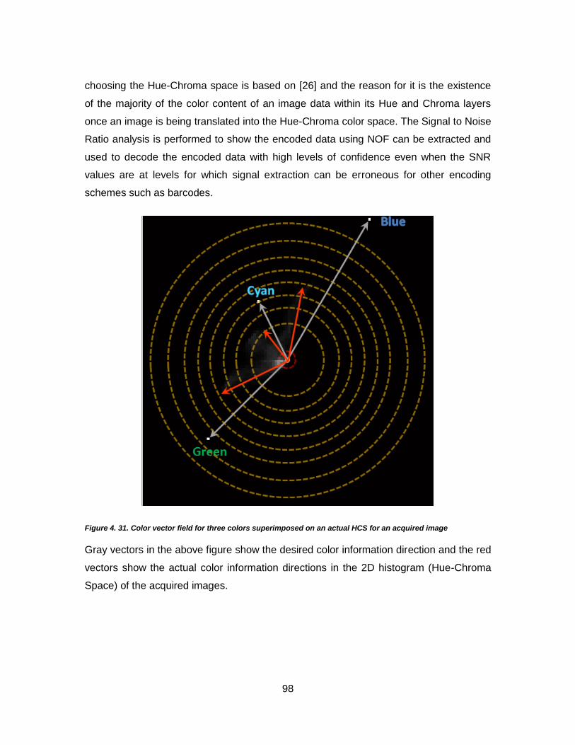
98

choosing the Hue-Chroma space is based on [26] and the reason for it is the existence

of the majority of the color content of an image data within its Hue and Chroma layers

once an image is being translated into the Hue-Chroma color space. The Signal to Noise

Ratio analysis is performed to show the encoded data using NOF can be extracted and

used to decode the encoded data with high levels of confidence even when the SNR

values are at levels for which signal extraction can be erroneous for other encoding

schemes such as barcodes.

Figure 4. 31. Color vector field for three colors superimposed on an actual HCS for an acquired image

Gray vectors in the above figure show the desired color information direction and the red

vectors show the actual color information directions in the 2D histogram (Hue-Chroma

Space) of the acquired images.

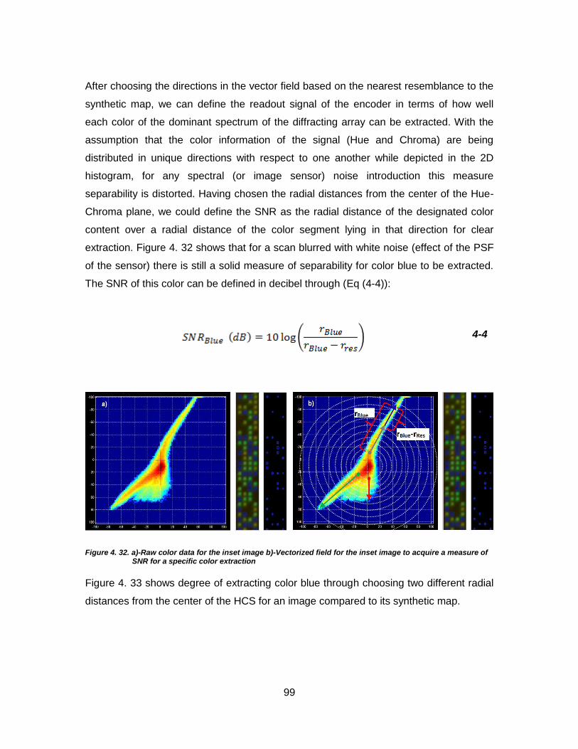
99

After choosing the directions in the vector field based on the nearest resemblance to the

synthetic map, we can define the readout signal of the encoder in terms of how well

each color of the dominant spectrum of the diffracting array can be extracted. With the

assumption that the color information of the signal (Hue and Chroma) are being

distributed in unique directions with respect to one another while depicted in the 2D

histogram, for any spectral (or image sensor) noise introduction this measure

separability is distorted. Having chosen the radial distances from the center of the Hue-

Chroma plane, we could define the SNR as the radial distance of the designated color

content over a radial distance of the color segment lying in that direction for clear

extraction. Figure 4. 32 shows that for a scan blurred with white noise (effect of the PSF

of the sensor) there is still a solid measure of separability for color blue to be extracted.

The SNR of this color can be defined in decibel through (Eq (4-4)):

4-4

Figure 4. 32. a)-Raw color data for the inset image b)-Vectorized field for the inset image to acquire a measure of SNR for a specific color extraction

Figure 4. 33 shows degree of extracting color blue through choosing two different radial

distances from the center of the HCS for an image compared to its synthetic map.

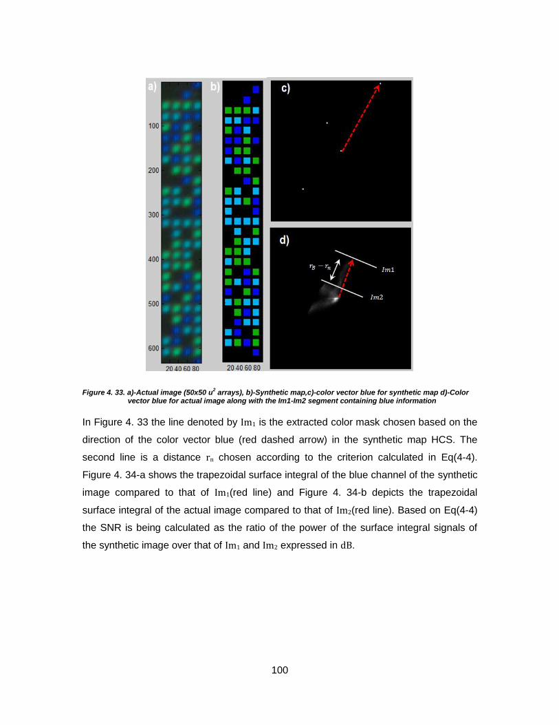
100

Figure 4. 33. a)-Actual image (50x50 u2 arrays), b)-Synthetic map,c)-color vector blue for synthetic map d)-Color

vector blue for actual image along with the Im1-Im2 segment containing blue information

In Figure 4. 33 the line denoted by Im1 is the extracted color mask chosen based on the

direction of the color vector blue (red dashed arrow) in the synthetic map HCS. The

second line is a distance rn chosen according to the criterion calculated in Eq(4-4).

Figure 4. 34-a shows the trapezoidal surface integral of the blue channel of the synthetic

image compared to that of Im1(red line) and Figure 4. 34-b depicts the trapezoidal

surface integral of the actual image compared to that of Im2(red line). Based on Eq(4-4)

the SNR is being calculated as the ratio of the power of the surface integral signals of

the synthetic image over that of Im1 and Im2 expressed in dB.

101

Figure 4. 34. a)-Surface integration of synthetic (blue) and color mask extracted at 0.7dB SNR b)-Surface integration of synthetic map(blue) and color mask extracted at 4.8 dB SNR

The SNR for Im1 is higher than that of Im2 due to presence of less noise compared to the

extracted color. Amid the low SNR for the acquired sample, the data recovery can still be

performed due to color-specific signal extraction (Figure 4. 35).

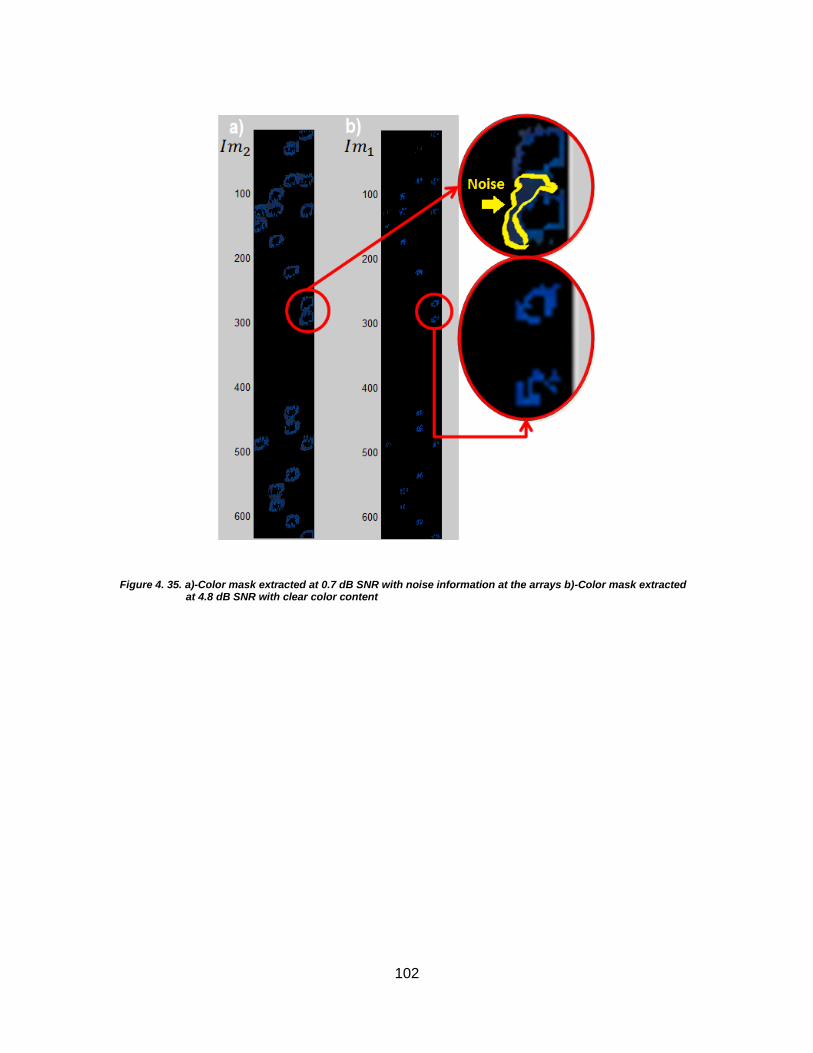
102

Figure 4. 35. a)-Color mask extracted at 0.7 dB SNR with noise information at the arrays b)-Color mask extracted at 4.8 dB SNR with clear color content

103

Chapter 5 Conclusion and Future Work

Through the course of this project we have designed, parameterized and fabricated an

optical unit information tagged as “NOF” (Nano-Optical-Feature) based on which an

encoding system along with a complete system level implementation design have been

presented. The actual storage density of NOF as an encoding unit information has been

investigated and measured through fabrication of various scales of NOF and analysis of

the readout signal in the form of RGB images. The work has focused on demonstrating

benefits of NOF-encoding comparing with finite-length storage media used commonly in

authentication industry. ID cards and in particular we focused on comparison with

commercial barcodes and magnetic stripe cards. The grounds for such comparison with

respect to shortcomings of the state of the art solutions have been investigated and NOF

has been proposed as a possible new generation of authentication storage media for

secure, machine readable data encoding with storage densities 4 to 400 times greater

than magnetic stripe standard cards in commercial use, depending on the feature

miniaturization (Table 7). The SNR for color-mask extraction has been employed as a

measure of signal reconstruction and it has been shown that through use of off-the-shelf

flatbed scanners with resolutions as high as 9600 dpi miniaturized encoded data can be

extracted in SNR values as low as 4.8 dB (Figure 4. 34). The latter allows for

commercial designs specialised for reading and decoding NOF encoded data with higher

precision and low costs due to the effective segmentation of the diffracted spectrum of

NOF. The conclusion to this work will be 1) a comparison between state of the art Nano-

optical-data encoding methods and the current project and future enhancements

possible to increase the storage density of the system, 2) Proof of concept for use of

plasmonic Nano-structures in data encoding and its advantages over state of the art

encoding schemes for authentication media, 3) a brief investigation on the effects of an

encoding unit information with more states of variation than binary bit on a transmitting

source with constant simple (non-complex) channel parameters.

104

5.1. Future Design for Security Performance of NOF Encoding System

State of the art Nano-optical encoding schemes regularly used in encoding data for CD

or DVD-BRDVD media use encryption algorithms such as DES (Data Encryption

Standard) in which the data and the encryption key are both present on the medium (the

CD or DVD). This allows for third party enthusiasts to be able to debug the encrypted file

into a binary file and rid the execution routine (main routine) from the subroutine(s) that

encrypts the file. In comparison to CD or DVD optical encoding, NOF presents an extra

level of security for the data. This extra security is the color-based signal extraction that

is necessary for the decoder to reconstruct the data. The use of NOF with different

grating periodicities makes it extremely difficult for the third party to mimic the encoded

data on a NOF secure medium due to the fact that a reader (decoder) reads the data

based on certain angle of reading. Having the reading angle and NOF periodicities in an

unknown state makes it impossible for an individual or program to merely guess the

pattern of the Nano-optical structures either from the colors they reflect or from the way

they are read by the detector. This extra security level is accompanied by the encryption

that NOF encoding algorithm imposes on the original data. The NOF encoder sets aside

a key or portion of the encrypted data that can be saved inside the reader (decoder)

hence allows for a key-lock security scheme. Compared to smart cards such as RFID

tags and magnetic stripe cards, NOF has a clear advantage regarding both data storage

density and security. RFID tags provide a storage density of maximum 165Kbits/in2 and

magnetic stripe cards‟ storage density is 2.87Kbits/in2 in its maximum condition. These

figures are much smaller than NOF storage density that under experimental conditions

and not well-tuned commercial conditions, allows for nearly one megabytes of data per

inch square (Table 7). Both magnetic stripe cards and RFID cards can be decrypted

using Differential Power Analysis (DPA) which is a side-channel attack that uses the chip

power consumption statistical data to decode the information on the cards. NOF data is

read and analyzed using image processing techniques (numerical analysis). Such

analysis does not leave a trace that can be picked up by a DPA process hence NOF

stands out both regarding its storage density and its security compared to the current ID

security cards [17] (Figure 5. 1).

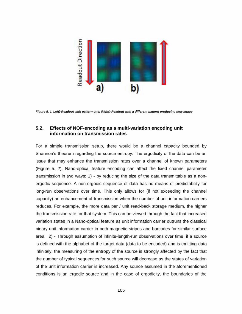
105

Figure 5. 1. Left)-Readout with pattern one; Right)-Readout with a different pattern producing new image

5.2. Effects of NOF-encoding as a multi-variation encoding unit information on transmission rates

For a simple transmission setup, there would be a channel capacity bounded by

Shannon‟s theorem regarding the source entropy. The ergodicity of the data can be an

issue that may enhance the transmission rates over a channel of known parameters

(Figure 5. 2). Nano-optical feature encoding can affect the fixed channel parameter

transmission in two ways: 1) - by reducing the size of the data transmittable as a non-

ergodic sequence. A non-ergodic sequence of data has no means of predictability for

long-run observations over time. This only allows for (if not exceeding the channel

capacity) an enhancement of transmission when the number of unit information carriers

reduces, For example, the more data per / unit read-back storage medium, the higher

the transmission rate for that system. This can be viewed through the fact that increased

variation states in a Nano-optical feature as unit information carrier outruns the classical

binary unit information carrier in both magnetic stripes and barcodes for similar surface

area. 2) - Through assumption of infinite-length-run observations over time; if a source

is defined with the alphabet of the target data (data to be encoded) and is emitting data

infinitely, the measuring of the entropy of the source is strongly affected by the fact that

the number of typical sequences for such source will decrease as the states of variation

of the unit information carrier is increased. Any source assumed in the aforementioned

conditions is an ergodic source and in the case of ergodicity, the boundaries of the

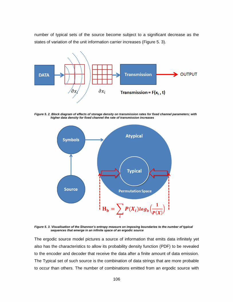
106

number of typical sets of the source become subject to a significant decrease as the

states of variation of the unit information carrier increases (Figure 5. 3).

Figure 5. 2. Block diagram of effects of storage density on transmission rates for fixed channel parameters; with higher data density for fixed channel the rate of transmission increases

Figure 5. 3. Visualisation of the Shannon’s entropy measure on imposing boundaries to the number of typical sequences that emerge in an infinite space of an ergodic source

The ergodic source model pictures a source of information that emits data infinitely yet

also has the characteristics to allow its probability density function (PDF) to be revealed

to the encoder and decoder that receive the data after a finite amount of data emission.

The Typical set of such source is the combination of data strings that are more probable

to occur than others. The number of combinations emitted from an ergodic source with

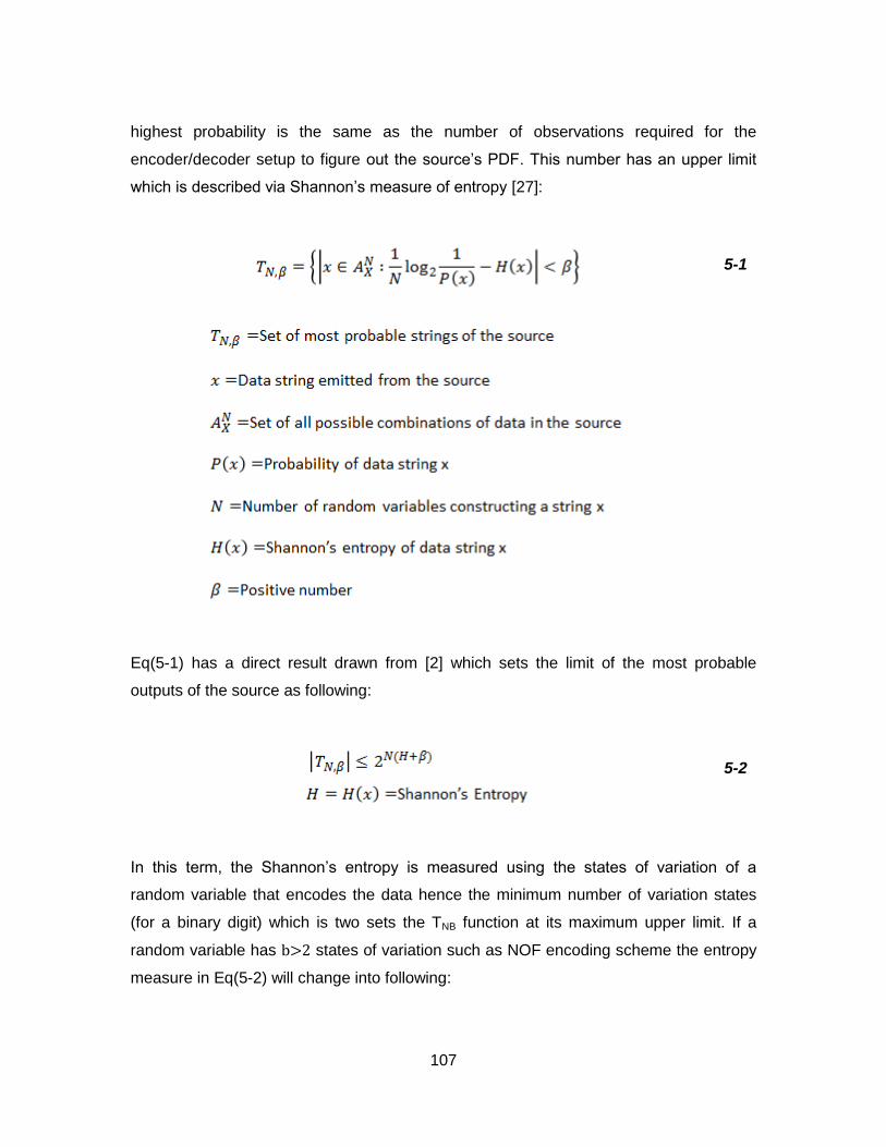
107

highest probability is the same as the number of observations required for the

encoder/decoder setup to figure out the source‟s PDF. This number has an upper limit

which is described via Shannon‟s measure of entropy [27]:

5-1

Eq(5-1) has a direct result drawn from [2] which sets the limit of the most probable

outputs of the source as following:

5-2

In this term, the Shannon‟s entropy is measured using the states of variation of a

random variable that encodes the data hence the minimum number of variation states

(for a binary digit) which is two sets the TNB function at its maximum upper limit. If a

random variable has b>2 states of variation such as NOF encoding scheme the entropy

measure in Eq(5-2) will change into following:

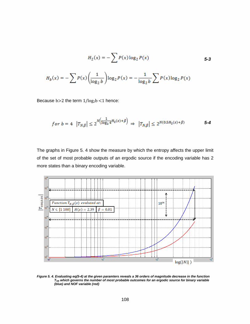
108

5-3

Because b>2 the term 1/log2b <1 hence:

5-4

The graphs in Figure 5. 4 show the measure by which the entropy affects the upper limit

of the set of most probable outputs of an ergodic source if the encoding variable has 2

more states than a binary encoding variable.

Figure 5. 4. Evaluating eq(5-4) at the given paramters reveals a 36 orders of magnitude decrease in the function TNB which governs the number of most probable outcomes for an ergodic source for binary variable (blue) and NOF variable (red)

109

5.3. Future Application of Multi-State Optical Encoding

Through the course of this work it has become clear that use of optical signals, as it has

been successfully trialed in advanced industries such as fine sensing and

telecommunication, and biomedical imaging can also be implemented in fields with less

application complexity and more cost-sensitive commercial sectors. The fact that a NOF

encoded text data can be stored in physical spaces about 100 times less than that of

any efficient barcodes and its ability to be passively yet securely read by specific readers

makes it a potential candidate for commercialization in the near future. The future work

on this topic will encompass combinatory algorithms that entail Nano-optical technology

along with more advanced mathematical models to fully resolve and employ benefits of a

multi-variation state optical unit information that can transmit data using angular

modulation of the incident wavelengths. Use of optical Nano-structures in order to

modulate analog properties of oscillating energy and waveforms can be a new way to

achieve multi-stage optical circuits (Figure 5. 5).

Figure 5. 5. Definition of a bit in a digital to analogue conversion circuit; the NOF or the Nano-optical feature can be viewed as having a variation state as a function of its periodicity

110

The effect of increasing the permutation space of one bit by having more than two

variation states not only affects the storage capacity of the storage device but also has

an impact on the arithmetic operators acting in the system. Figure 5. 6-(a) shows a

series of logical gates and their overall result in node E whereas Figure 5. 6-(b) shows

the same junction when the last gate produces more than two states:

Figure 5. 6. a) - NOR gate using classical Boolean operands b) - NOR gate using a multi-varied state bit in combination with Boolean operands

The second multi-varied bit (bit B) can control a different set of logical gates. The latterly

mentioned is in the case of logical gates (acting in a Boolean framework) and not gates

that can also generate multiple responses to various sets of inputs. Investigation of

combining non-logical gates (gates with more than one response) and multi-state bits is

one of the potential scopes of this work yet alongside increase of complexity; the size of

such combinations will decrease significantly. The computation speed will also benefit

from having non logical gates and multi-state bits since more complex arithmetic

operations can take place within smaller sequences of gates and bits. Having described

the advantages of multi-state bit it is necessary to mention that in order for the concept

to be functional the states of variation must be both distinct and reproducible with high

degree of accuracy.

111

References

112

[1] S. Vosoogh-Grayli, Diffractive Nano-Structures as Optical Visual and Machine Readable Features, 2012, Master Thesis.

[2] K. Sayood, An Introduction to Data Compression, 2nd ed., K. Sayood, Ed. San Francisco, USA: Morgan Kaufmann, 2006.

[3] V.S.Bagad I.A.Dhotre, Data Communication, 1st ed., I.A.Dhotre, Ed. Pune, India: Technical Publications, 2008.

[4] R. Bangia, Dictionary of Information Technology, 2nd ed., R. Bangia, Ed. New Dehli India: Laxmi Publications, 2010.

[5] A. Godse D.A.Godse, Digital Techniques, 1st ed., D.A.Godse, Ed. Pune, India: Technical Publications, 2008.

[6] R. L. Goodstein, Boolean Algebra, 1st ed., R. L. Goodstein, Ed. New York, USA: Dover Publications, 2007.

[7] S. Bathul, Mathematical Foundations of Computer Science, 1st ed., S. Bathul, Ed. New Delhi, India: PHI Publication, 2010.

[8] J. B. Anderson, Source and Channel Coding: An Algorithmic Approach, 1st ed., J. B. Anderson, Ed. Norwell, USA: Kluwer Academic Publisher Group, 1991.

[9] A. Khurshudov, The Essential Guide to Computer Data Storage, 1st ed., A. Khurshudov, Ed. Saddle River, USA: Prentice Hall, 2001.

[10] E. Meinders, Optical Data Storage: Phase Change Media and Recording, 1st ed., E. Meinders, Ed. Dordrecht, Netherlands: Springer verlag, 2006.

[11] S. K. Singh, Database Systems: Concepts, Design & Applications, 1st ed., S. K. Singh, Ed. New Delhi, India: Pearson Education, 2009.

[12] R. W. Ditchburn, Light, 1st ed., R. W. Ditchburn, Ed. New York, USA: Dover Publications Inc., 1991.

[13] J. A. Stratton, Electromagnetic Theory, 1st ed., J. Audino, Ed. New Jersey, USA: Wiley and Sons, 2007.

[14] (2012, Jan.) Adams Communications. [Online] http://www.adams1.com/39code.html

[15] (1995, September) Adams Communications Introduction to Barcodes. [Online]. http://www.adams1.com/stack.html

113

[16] (2012, September) Zebra Technologies Online Introduction to RFID Tags. [Online]. http://www.zebra.com/us/en/solutions/getting-started/rfid-printing-encoding/rfid-tag- characteristics.html

[17] W. Rankl, Smart Card Handbook, 4th ed., W. Rankl, Ed. West Sussex, UK: Wiley & Sons, 2010.

[18] H. Lehpamer, RFID Design and Principles, 2nd ed., H. Lehpamer, Ed. Norwood, USA: Artech House, 2012.

[19] E.G. Loewen, Diffraction Gratings and Applications, 1st ed., E.G. Loewen, Ed. New York, USA: Marcel Dekker Inc., 1997.

[20] R. Gordon, "A New Generation of Sensors Based on Extraordinary Optical Transmission," Accounts of Chemical Research, vol. 41, no. 8, pp. 1049-1057, July 2008. [21] R.V. Baltz, "Surface Plasmons in Bulk Metals and Metalic Clusters and Metalic Heterostructures," Spectroscopy and Dynamics of Collective Excitations in Solids, vol. 356, pp. 1-36, 1997.

[22] R.Gonzales, Digital Image Processing, 2nd ed., R.Gonzales, Ed. Saddle River, USA: Prentice Hall, 2002.

[23] S. Eddins, Freehand Segmentation in a*-b* Plane, 2011, Steve Eddins Blogs on Image Processing using MATLAB.

[24] M. Savoini, "All-optical subdiffraction multilevel data encoding onto azo- polymeric thin films," Optics Letters, vol. 34, no. 6, pp. 761-763, March 2009.

[25] S. W. Birtwell, "Superimposed Nano-scale Diffraction Gratings as High Capacity Barcodes for Biological and Chemical Applications," Optics in Life Science, vol. 281, no. 7, pp. 1789-1795, October 2007.

[26] G. Sharma, Digital Imaging : Handbook, 2nd ed., G. Sharma, Ed. Florida, United States: CRC Press, 2003.

[27] T. M. Cover, Elements of Information Theory, 2nd ed., T. M. Cover, Ed. New Jersey, USA: John Wiley & Sons, 1991.

[28] A. Ghatak, Optics, 4th ed., A. Ghatak, Ed. New Delhi, India: McGraw-Hill, 2009.

[29] T. W. Ebbesen, "Light in Tiny Holes," Nature Physics, vol. 445, pp. 39-46, January 2007.

[30] M. Mrejen, Investigating the Confinement of Light in Nanometric Domain, May 2007,

114

Master's Thesis from The Hebrew University of Jerusalem.

[31] M. Mansuripour, Classical Optics, 1st ed., M. Mansuripour, Ed. Cambridge, UK: Cambridge University Press, 2002.

[32] A. Zayats, "Nano Optics of Surface Plasmon Plaritons," Physics Reports, vol. 408, no. 3-4, pp. 131-314, March 2005.

[33] S. Dror, Modern Introduction to Surface Plasmons, 1st ed., S. Dror, Ed. Cambridge, UK: Cambrdige University Press, 2010.

[34] S. Kawata, Near-Field Optics and Surface Plasmon Polaritons, 1st ed., M. Ohtsu, Ed. Berlin, Germany: Springer, 2001.

[35] S. Rodrigo, "Influence of Material Properties on Extraordinary Optical Transmission Through Hole Arrays," Physical Review, vol. 77, no. 7, February 2008.

[36] L. Novotny, Principles of Nano Optics, 1st ed., L. Novotny, Ed. Cambridge, UK: Cambridge University Press, 2006.

[37] Z. Cui, Nano Fabrication: Priniciples, Capabilities and Limits, 1st ed., Z. Cui, Ed. New York, USA: Springer Verlag, 2008.

[38] D. MacKay, Information Theory, Inference, and Learning Algorithms, 1st ed., D. MacKay, Ed. Cambridge, UK: Cambridge University Press, 2003.

[39] M. Erickson, Number Theory, 1st ed., M. Erickson, Ed. Boca Raton, USA: CRC Press, 2008.

[40] F. Saadia, "Canalizing Zhegalkin Polynomials as Models for Gene Expression Time Series Data," in Engineering of Intelligent Systems, 2006 IEEE International Conference, Islamabaad, 2006.

115

Appendices

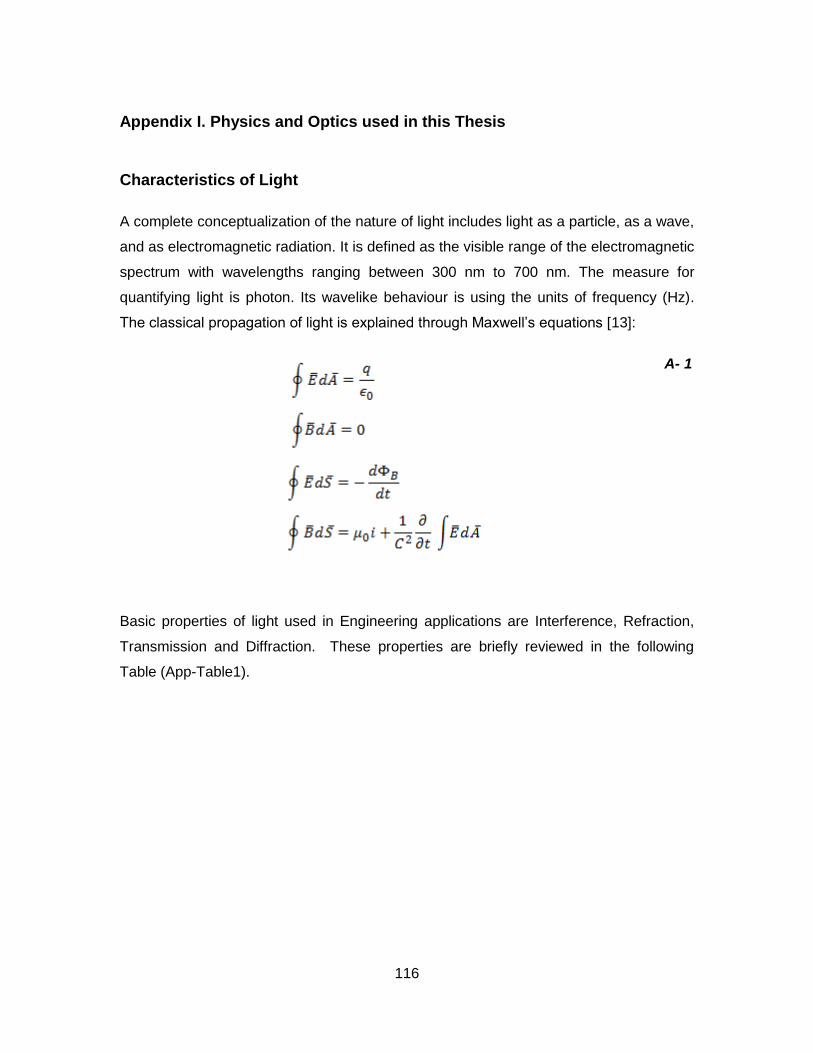
116

Appendix I. Physics and Optics used in this Thesis

Characteristics of Light

A complete conceptualization of the nature of light includes light as a particle, as a wave,

and as electromagnetic radiation. It is defined as the visible range of the electromagnetic

spectrum with wavelengths ranging between 300 nm to 700 nm. The measure for

quantifying light is photon. Its wavelike behaviour is using the units of frequency (Hz).

The classical propagation of light is explained through Maxwell‟s equations [13]:

A- 1

Basic properties of light used in Engineering applications are Interference, Refraction,

Transmission and Diffraction. These properties are briefly reviewed in the following

Table (App-Table1).

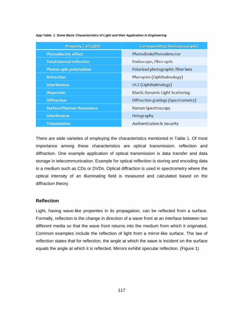
117

App-Table. 1. Some Basic Characteristics of Light and their Application in Engineering

There are wide varieties of employing the characteristics mentioned in Table 1. Of most

importance among these characteristics are optical transmission, reflection and

diffraction. One example application of optical transmission is data transfer and data

storage in telecommunication. Example for optical reflection is storing and encoding data

in a medium such as CDs or DVDs. Optical diffraction is used in spectrometry where the

optical intensity of an illuminating field is measured and calculated based on the

diffraction theory.

Reflection

Light, having wave-like properties in its propagation, can be reflected from a surface.

Formally, reflection is the change in direction of a wave front at an interface between two

different media so that the wave front returns into the medium from which it originated.

Common examples include the reflection of light from a mirror-like surface. The law of

reflection states that for reflection, the angle at which the wave is incident on the surface

equals the angle at which it is reflected. Mirrors exhibit specular reflection. (Figure 1)

118

Figure 1. Angle of incidence and reflection are equal when a wave front (light) arrives at a mirror-like surface (θI is the incidence angle and θr is the reflection angle)

Refraction

Refraction is the bending of light as it passes between materials of different density. The

index of refraction of a material is the ratio of the speed of light in vacuum to the speed

of light in that material [28]. Eq(2-2) quantifies this as follows:

A- 2

The more dense the material is the slower the speed of light in that material thus n > 1

for all materials and increases with increasing density. In vacuum n is equal to one. The

frequency of light does not change when it passes from one medium to another.

According to the formula v = λf , the wavelength must change (f is the angular frequency

of light). The index of refraction can therefore be written in terms of wavelengths (Figure

2):

119

A- 3

Figure 2. Schematic of optical refraction

The change in speed and wavelength at the boundary between two materials causes

light to change direction. If θ1 is the angle of the ray relative to the normal to the surface

in medium 1 , and θ2 is the angle relative to the normal in medium 2, then:

A- 4

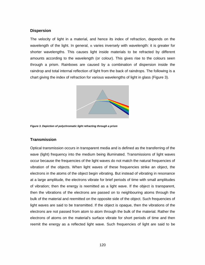
120

Dispersion

The velocity of light in a material, and hence its index of refraction, depends on the

wavelength of the light. In general, n varies inversely with wavelength: it is greater for

shorter wavelengths. This causes light inside materials to be refracted by different

amounts according to the wavelength (or colour). This gives rise to the colours seen

through a prism. Rainbows are caused by a combination of dispersion inside the

raindrop and total internal reflection of light from the back of raindrops. The following is a

chart giving the index of refraction for various wavelengths of light in glass (Figure 3).

Figure 3. Depiction of polychromatic light refracting through a prism

Transmission

Optical transmission occurs in transparent media and is defined as the transferring of the

wave (light) frequency into the medium being illuminated. Transmissions of light waves

occur because the frequencies of the light waves do not match the natural frequencies of

vibration of the objects. When light waves of these frequencies strike an object, the

electrons in the atoms of the object begin vibrating. But instead of vibrating in resonance

at a large amplitude, the electrons vibrate for brief periods of time with small amplitudes

of vibration; then the energy is reemitted as a light wave. If the object is transparent,

then the vibrations of the electrons are passed on to neighbouring atoms through the

bulk of the material and reemitted on the opposite side of the object. Such frequencies of

light waves are said to be transmitted. If the object is opaque, then the vibrations of the

electrons are not passed from atom to atom through the bulk of the material. Rather the

electrons of atoms on the material's surface vibrate for short periods of time and then

reemit the energy as a reflected light wave. Such frequencies of light are said to be

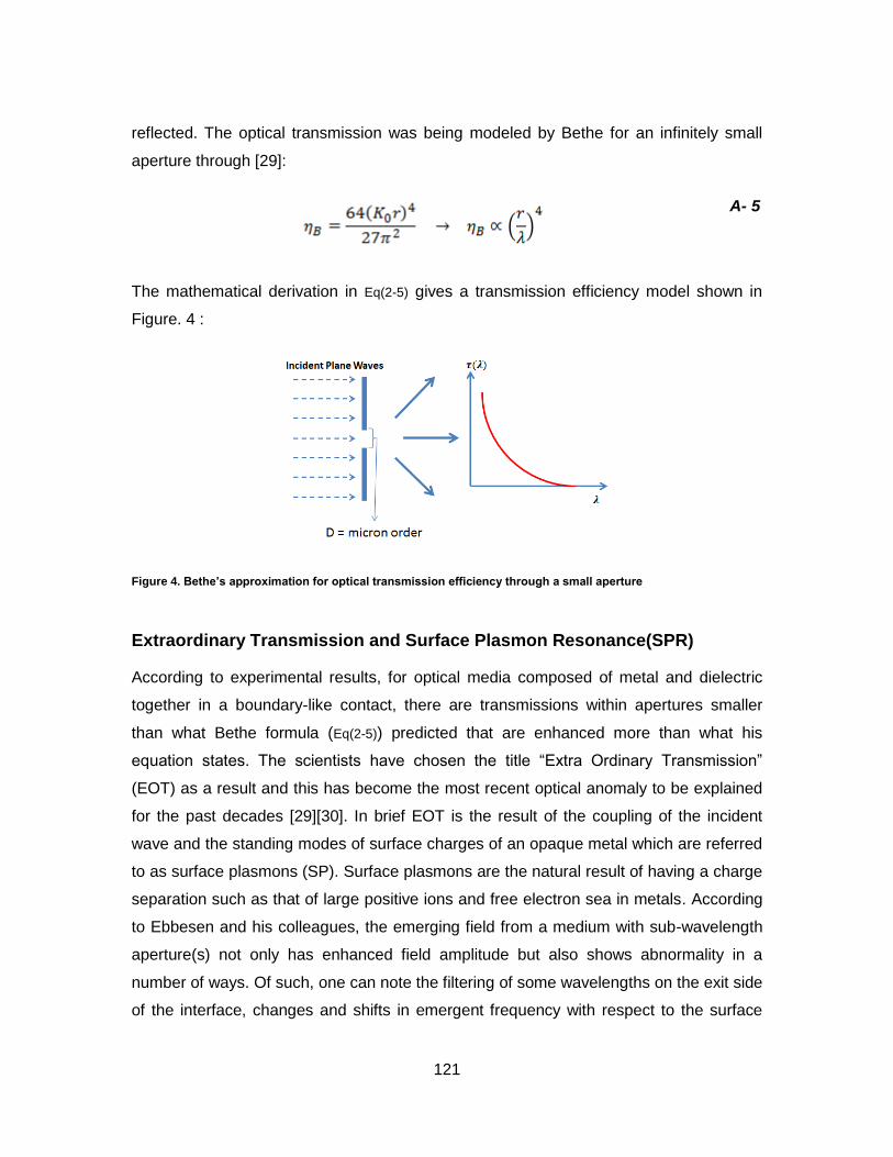
121

reflected. The optical transmission was being modeled by Bethe for an infinitely small

aperture through [29]:

A- 5

The mathematical derivation in Eq(2-5) gives a transmission efficiency model shown in

Figure. 4 :

Figure 4. Bethe’s approximation for optical transmission efficiency through a small aperture

Extraordinary Transmission and Surface Plasmon Resonance(SPR)

According to experimental results, for optical media composed of metal and dielectric

together in a boundary-like contact, there are transmissions within apertures smaller

than what Bethe formula (Eq(2-5)) predicted that are enhanced more than what his

equation states. The scientists have chosen the title “Extra Ordinary Transmission”

(EOT) as a result and this has become the most recent optical anomaly to be explained

for the past decades [29][30]. In brief EOT is the result of the coupling of the incident

wave and the standing modes of surface charges of an opaque metal which are referred

to as surface plasmons (SP). Surface plasmons are the natural result of having a charge

separation such as that of large positive ions and free electron sea in metals. According

to Ebbesen and his colleagues, the emerging field from a medium with sub-wavelength

aperture(s) not only has enhanced field amplitude but also shows abnormality in a

number of ways. Of such, one can note the filtering of some wavelengths on the exit side

of the interface, changes and shifts in emergent frequency with respect to the surface

122

parameters (boundary surface), intensity highs and lows proportional to the geometry of

the sub-wavelength apertures and etc [29]. These effects can be in brief linked to a

hypothesis that has been dedicated to the existence of a fundamental frequency of the

bulk plasma that exists within a metallic element. These oscillations are in turn also

sources for charge induction as every charged particle is a source of electric field itself.

The quantum mechanical definition of this model quantizes the plasma oscillations into

quanta called plasmons. Plasmons and their network give rise to the hypothesis of

surface charges which are in fact lower in energy compared to those plasmons in the

bulk and are limited by a surface boundary between the metal and some other medium

(usually a dielectric medium such as air). These surface charges are termed as surface

plasmons. Surface plasmon as indicated by [31] is also regarded as a solution

(inhomogeneous) to the Maxwell‟s equation for the boundary conditions imposed on it

based on the differences of permittivity in two different media. Of the two usually one has

positive and one has negative permittivity. The metals have negative permittivity and a

dielectric e.g. air surrounding the metal provides the positive value. Here the analogy is

to understand the nature of surface plasmons as an evanescent mode of electric field

dependent on the plasma frequency of the bulk material and the charge density at the

surface of the metal [32]. The actual interest is when these modes become radiative

and/or penetrate the metal. The aforementioned is the explanation of what opposes

Bethe‟s prediction for the emergence of an enhanced field through a sub-wavelength

aperture. Because in an isotropic medium such as a metal the permittivity is in fact a

function of the wave vector in that medium and the index of refraction, for indices of

refraction much smaller than the wave number a large negative permittivity condition for

one side of a boundary is automatically satisfied through metals [33]. This in turns allows

for the existence of standing surface plasmon modes. It becomes a matter of interest

when the surface plasmons couple with an incident photon and turn into surface

plasmon polaritons [34]. It is necessary to say that in some texts the term surface

plasmon and surface plasmon polariton are being used interchangeably whereas here

the work tries to separate the non-propagative modes from the propagative ones through

surface plasmon (SP) and surface plasmon polariton (SPP) respectively. The term used

in literature for this interaction is “resonant absorption” and the reason for this is that the

momentum of the incoming photon must match the wave number of the plasmon in

order for allowance of any further modes be it decaying through radiation or through

123

absorption into the metal [32]. The fact that the wave number of the incident photon must

match that of the plasmon (surface plasmon) indicates a resonance. In order to resonate

and excite the SP modes, an incident plane wave must be carrying enough amplitude

into the space (air) in order to reach the metal with enough energy for excitation.

Thereby one must “force” the metal to accept the incoming wave and hence allow for a

propagative mode of the surface plasmons known as surface plasmon polaritons.(Figure

5)

Figure 5. 3D model of plasma oscillation, incidence field and surface plasmon polariton generation. The direction of the SPP is a function of parallel component of the incident field

124

Surface plasmon resonance (SPR) is the resonant, collective oscillation of valence in the

metal stimulated by incident light. The resonance condition is established when the

frequency of light photons matches the natural frequency of surface electrons oscillating

against the restoring force of positive nuclei. SPR in nanometer-sized structures is called

localized surface plasmon resonance. In order to excite surface plasmons in a resonant

manner, one can use an electron or light beam (visible and infrared are typical). The

incoming beam has to match its momentum to that of the plasmon. In the case of p-

polarized light (polarization occurs parallel to the plane of incidence. S-polarized light

(polarization occurs perpendicular to the plane of incidence) cannot excite electronic

surface plasmons. Surface plasmons obey the following dispersion relation

[34][35](Figure 6):

A- 6

Figure 6. Evanescent or standing modes of the surface plasmon electric field distribution

125

Diffraction

Diffraction is the apparent "bending" of light waves around obstacles in its path. This

bending is due to Huygens‟s principle, which states that all points along a wave front act

as if they were point sources. Thus, when a wave comes against a barrier with a small

opening, all but one of the effective point sources are blocked, and the light coming

through the opening behaves as a single point source, so that the light emerges in all

directions, instead of just passing straight through the slit [28] (Figure 7).

Figure 7. Diffracting light (wavefront) through a small aperture (slit)

The intensity of the diffracted optical field due to the presence of an aperture is

calculated through the following equations (Figure 8):

A- 7

126

Figure 8. A graph based on the amplitude and intensity distribution of the diffracted field

Types of Diffraction

There are two types of optical diffraction that are related yet the amplitude and optical

intensity related to them are different from one another. These types are 1)-Fresnel

Diffraction and 2)-Fraunhofer Diffraction (Figure 9). The main factor that determines the

type of diffracting system is the distance at which the optical field is being imaged or

sensed. Fresnel diffraction can be summarized in an integral form using an arbitrary

aperture as shown in Figure 10. The optical intensity describing the Fresnel diffraction is

calculated through [28]:

A- 8

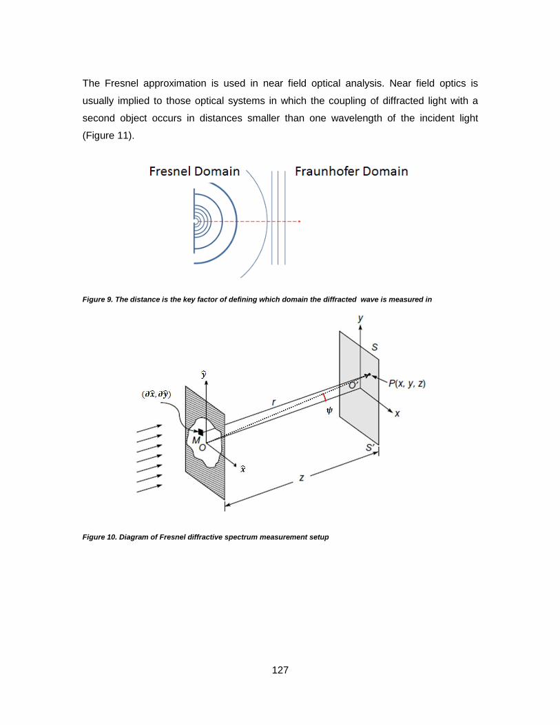
127

The Fresnel approximation is used in near field optical analysis. Near field optics is

usually implied to those optical systems in which the coupling of diffracted light with a

second object occurs in distances smaller than one wavelength of the incident light

(Figure 11).

Figure 9. The distance is the key factor of defining which domain the diffracted wave is measured in

Figure 10. Diagram of Fresnel diffractive spectrum measurement setup

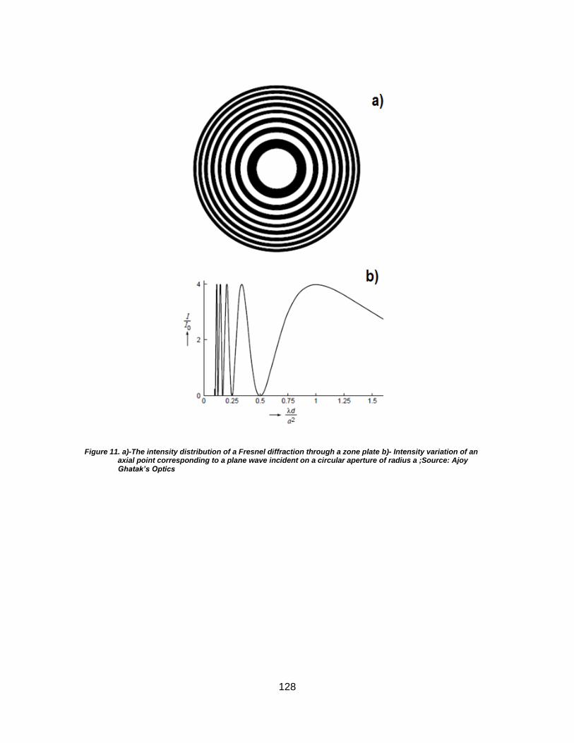
128

Figure 11. a)-The intensity distribution of a Fresnel diffraction through a zone plate b)- Intensity variation of an axial point corresponding to a plane wave incident on a circular aperture of radius a ;Source: Ajoy Ghatak’s Optics

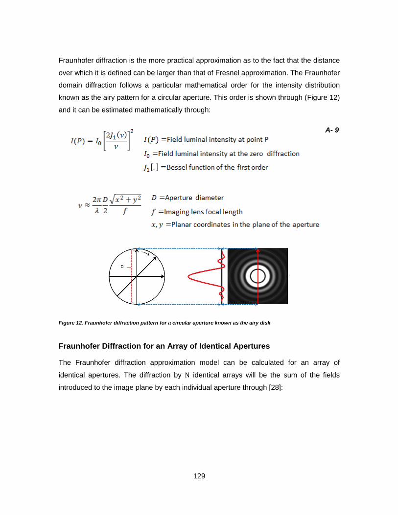
129

Fraunhofer diffraction is the more practical approximation as to the fact that the distance

over which it is defined can be larger than that of Fresnel approximation. The Fraunhofer

domain diffraction follows a particular mathematical order for the intensity distribution

known as the airy pattern for a circular aperture. This order is shown through (Figure 12)

and it can be estimated mathematically through:

A- 9

Figure 12. Fraunhofer diffraction pattern for a circular aperture known as the airy disk

Fraunhofer Diffraction for an Array of Identical Apertures

The Fraunhofer diffraction approximation model can be calculated for an array of

identical apertures. The diffraction by N identical arrays will be the sum of the fields

introduced to the image plane by each individual aperture through [28]:

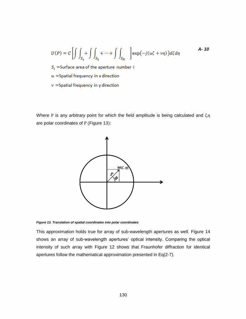
130

A- 10

Where P is any arbitrary point for which the field amplitude is being calculated and ζ,η

are polar coordinates of P (Figure 13):

Figure 13. Translation of spatial coordinates into polar coordinates

This approximation holds true for array of sub-wavelength apertures as well. Figure 14

shows an array of sub-wavelength apertures‟ optical intensity. Comparing the optical

intensity of such array with Figure 12 shows that Fraunhofer diffraction for identical

apertures follow the mathematical approximation presented in Eq(2-7).

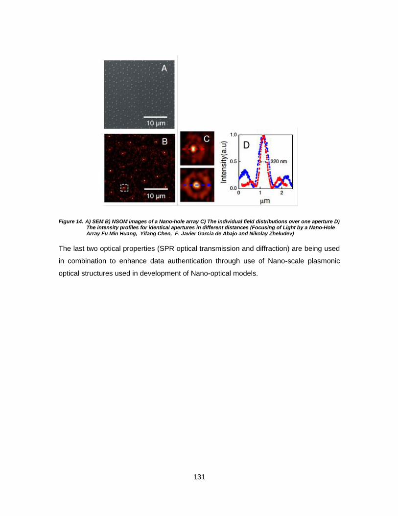
131

Figure 14. A) SEM B) NSOM images of a Nano-hole array C) The individual field distributions over one aperture D) The intensity profiles for identical apertures in different distances (Focusing of Light by a Nano-Hole Array Fu Min Huang, Yifang Chen, F. Javier Garcia de Abajo and Nikolay Zheludev)

The last two optical properties (SPR optical transmission and diffraction) are being used

in combination to enhance data authentication through use of Nano-scale plasmonic

optical structures used in development of Nano-optical models.

132

Nano Optical Design and Plasmonic Structures

Nano optics‟ is the collection of techniques by means of which optical convergence can

be recorded in lengths beyond the diffraction limit. Some of the notable applications that

arise from the latterly mentioned extension are super-resolution microscopy and ultra-

high-density optical data storage. It also gives rise to the fabrication process of sub-wave

length optical structures known as plasmonic structures. These structures due to being

below the wavelength of an incident light can guide and manipulate the visible light in

sub-wavelength systems. Such manipulation allows for harvesting signals which are

capable of travelling longer than expected distances in the Nano-order structures.

Definition of Nano-optical design can be interpreted as enhancing the optical space or

optical confinement required for a photon through modification of surface parameters

such as roughness, thickness, index of refraction etc. Quite simplified, the propagation of

light in free space obeys a conservative law as in the following equation [36]:

A- 11

And the immediate result of Eq(2-11) is a limit for wave solutions to exist through:

A- 12

Eq(2-12) shows that there will spatial confinement for a propagating quasi particle such as

a photon due to the spread of its wave vector in different directions or in brief, under

certain angles or beyond certain lengths a particular wave simply, cannot exist. Nano

optics and Nano-optical design generally can be said to be dealing with the problem of

spatial confinement of photons with respect to different propagation modes and tends to

find solutions (analytical and empirical) to enhance and increase the confinement

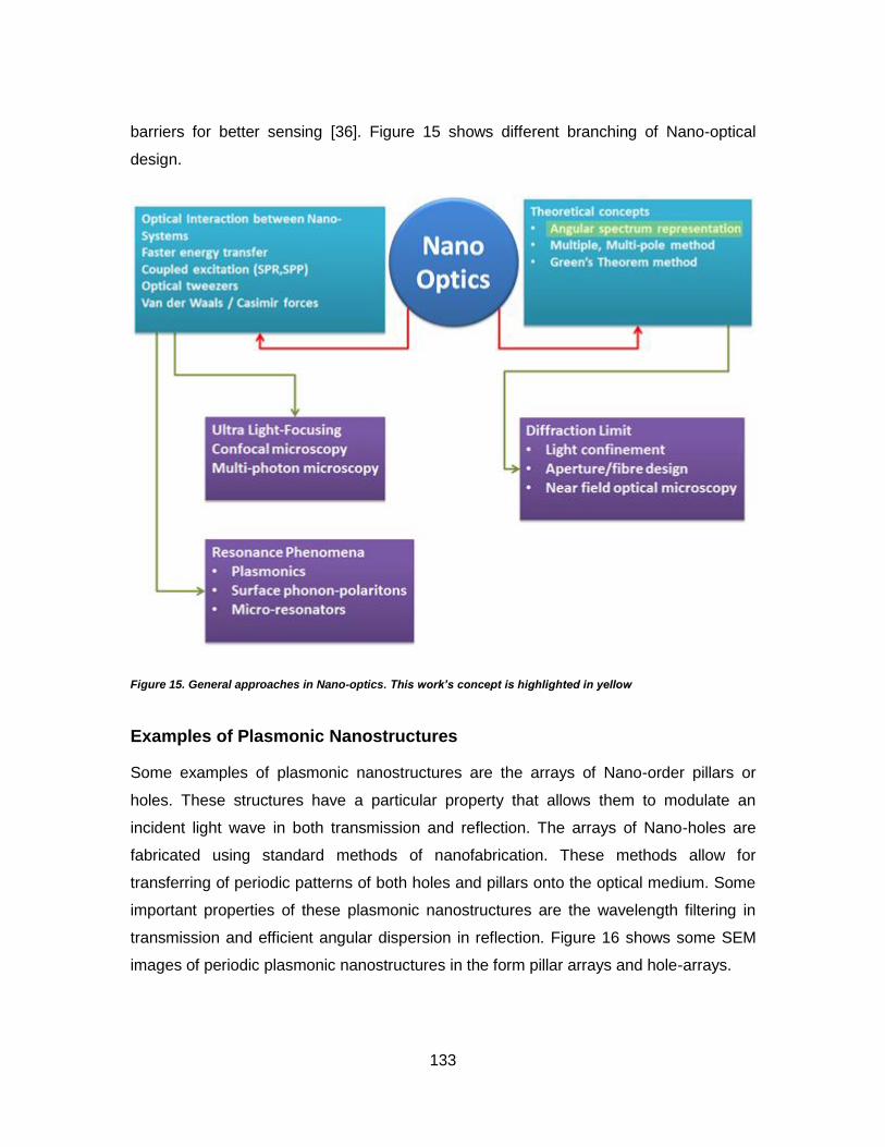
133

barriers for better sensing [36]. Figure 15 shows different branching of Nano-optical

design.

Figure 15. General approaches in Nano-optics. This work’s concept is highlighted in yellow

Examples of Plasmonic Nanostructures

Some examples of plasmonic nanostructures are the arrays of Nano-order pillars or

holes. These structures have a particular property that allows them to modulate an

incident light wave in both transmission and reflection. The arrays of Nano-holes are

fabricated using standard methods of nanofabrication. These methods allow for

transferring of periodic patterns of both holes and pillars onto the optical medium. Some

important properties of these plasmonic nanostructures are the wavelength filtering in

transmission and efficient angular dispersion in reflection. Figure 16 shows some SEM

images of periodic plasmonic nanostructures in the form pillar arrays and hole-arrays.

134

Figure 16. A) Plasmonic nanostructures in the form of Nano-pillars and B)-Nano-hole arrays

Nano-Fabrication Techniques for Fabrication of plasmonic nanostructures

An introduction to what generally encompasses nanofabrication can be as briefly as the

following sentence from [37] : “Nano fabrication evolves from micro fabrication, and

since the advent of first transistors in 1947, the IC industry has been the main driving

force to continuously push fabrication technologies to their new dimensional limits”. The

general purpose of a nanofabrication process is being schematically depicted in the

following block diagram highlighting the technique used in this work in red outline [37]

(Table 9):

Table 9. Fundamentals of Nano fabrication for optics (Nanofabrication: Principles, Capabilities and Limits by Zheng Cui)

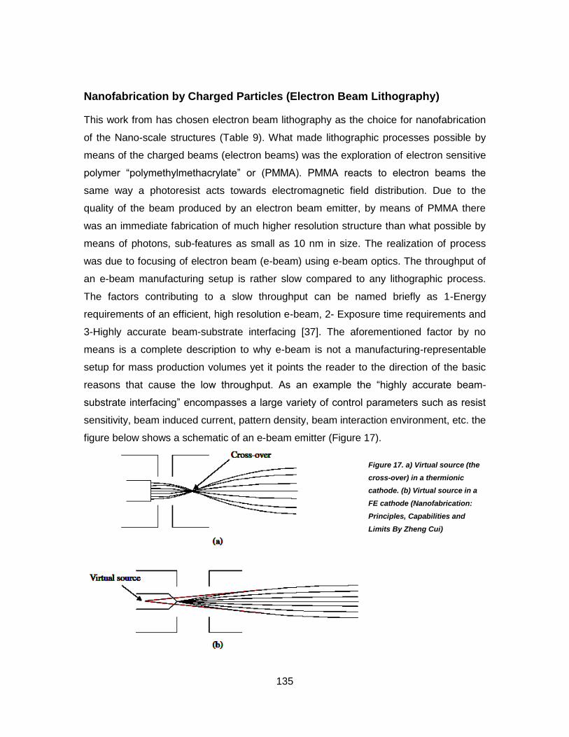
135

Nanofabrication by Charged Particles (Electron Beam Lithography)

This work from has chosen electron beam lithography as the choice for nanofabrication

of the Nano-scale structures (Table 9). What made lithographic processes possible by

means of the charged beams (electron beams) was the exploration of electron sensitive

polymer “polymethylmethacrylate” or (PMMA). PMMA reacts to electron beams the

same way a photoresist acts towards electromagnetic field distribution. Due to the

quality of the beam produced by an electron beam emitter, by means of PMMA there

was an immediate fabrication of much higher resolution structure than what possible by

means of photons, sub-features as small as 10 nm in size. The realization of process

was due to focusing of electron beam (e-beam) using e-beam optics. The throughput of

an e-beam manufacturing setup is rather slow compared to any lithographic process.

The factors contributing to a slow throughput can be named briefly as 1-Energy

requirements of an efficient, high resolution e-beam, 2- Exposure time requirements and

3-Highly accurate beam-substrate interfacing [37]. The aforementioned factor by no

means is a complete description to why e-beam is not a manufacturing-representable

setup for mass production volumes yet it points the reader to the direction of the basic

reasons that cause the low throughput. As an example the “highly accurate beam-

substrate interfacing” encompasses a large variety of control parameters such as resist

sensitivity, beam induced current, pattern density, beam interaction environment, etc. the

figure below shows a schematic of an e-beam emitter (Figure 17).

Figure 17. a) Virtual source (the

cross-over) in a thermionic

cathode. (b) Virtual source in a

FE cathode (Nanofabrication:

Principles, Capabilities and

Limits By Zheng Cui)

136

An electron has the capacity of occupying a whole of a three dimensional confinement

the same way as it can interact and coexist with millions of other electrons in the matter.

The propagative nature of electron makes it a point source which has to obey the

Maxwell conditions hence act as spherical radiative source when accelerated. For

achieving small in diameter electron beams one must resolve the conditions through

electron optics [37]. The electron-beam systems employ a rotationally-symmetric electro-

static field in which the behaviour of a charged particle obeys the Lorentz force given by

(Figure 18):

A- 13

Figure 18. An electrical field of 2nd

order symmetry forming a lens for charged particles

137

Any charged particle in the system will experience a radial pull r that drags it towards the

center of the beam and an acceleration that acts in the Z (direction of beam propagation)

direction. It is the radial pull that converges the beam into a focus (Figure 19).

Figure 19. The radial and axial force generate a rotational profile around the axis

In Nano-fabrication technology the pattern transfer is not the final stage of a design. In

all of the cases the patterns after being deposited on a sacrificial layer such as the

photoresist or electron sensitive PMMA need to be immersed in chemical etchants that

dispose of unwanted layers. This post processing includes two major types of chemical

etchants and relies on the crystalline structure of the processed materials for correct and

ordered disposal of the materials. In general there are two types of etching processes

[37]:

1-Wet etching: material is immersed in the etchant solution and reactive layers dissolve

2-Dry etching: material is being exposed to sputtering and reactive gases for sublimation

During a wet etching process the dissolution may tackle the layers in an either isotropic

or anisotropic manner. The isotropic dissolution creates so called “craters” or “edge

138

effects” under the mask in use whereas the anisotropic etching results in geometrically

aligned sides (crystalline structure limits the dissolution) and hence can be used to

create bridges between structures. Dry etching can be classified into three main classes

termed as Reactive Ion Gas (RIE), Sputter etching and vapour phase etching. In RIE in

brief the substrate is exposed to a mixture of chemical gases wherein a plasma spark

produces ion masses that start reacting with substrate molecules. The mechanism of

sputtering is rather similar to that sputter deposition with the difference in the substrate

being “bombarded” by non-reactive ions. The etching parameters are quite similar to RIE

in principle. Vapour phase etching is another dry etching method, which can be done

with simpler equipment than what RIE requires. In this process the wafer to be etched is

placed inside a chamber, in which one or more gases are introduced. The material to be

etched is dissolved at the surface in a chemical reaction with the gas molecules. The two

most common vapour phase etching technologies are silicon dioxide etching using

hydrogen fluoride (HF) and silicon etching using xenon di-fluoride (XeF2), both of which

are isotropic in nature [37]. Nano fabrication processes described earlier have all one

goal in common and that of delivering an accurate enough a profile for the designed

Nano-structures. If the design is requiring high accuracy pattern transfer then the

process must also become subject to more steps and more phases in order to deliver

the required level of accuracy in the pattern transfer. Below is a strip describing one

application of a combination of charged particle (E-beam) pattern transfer and wet

etching post processing with the aims of delivering arrays of Nano-scale gratings with

circular aperture profiles. This work has been the experimental foundation of the current

study and the aim as will be discussed in detail in the coming chapters, has been to

fabricate small size (few 100 micron) surface area with grating patterns that are excitable

by different wavelengths of visible portion of the electromagnetic spectrum. As much

said as in this process, the overall excitation of the surface area under grating is more

important than aperture design. This means that an overall uniformity of the apertures

would be attempted whereas an exact circular pattern (with absolutely no deformity) is

not a primary issue [37] (Figure 20).

139

Figure 20. Schematic of fabrication process for arrays of nano grooves (nano holes)

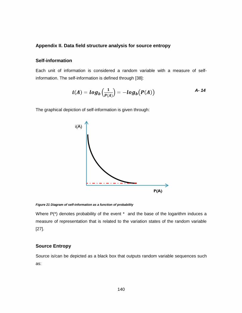
140

Appendix II. Data field structure analysis for source entropy

Self-information

Each unit of information is considered a random variable with a measure of self-

information. The self-information is defined through [38]:

A- 14

The graphical depiction of self-information is given through:

Figure 21 Diagram of self-information as a function of probability

Where P(*) denotes probability of the event * and the base of the logarithm induces a

measure of representation that is related to the variation states of the random variable

[27].

Source Entropy

Source is/can be depicted as a black box that outputs random variable sequences such

as:

141

Figure 22 Source of information as a black box outputting sequences of random variables

Entropy is the average self-information of a random variable. In other words, the average

self-information is the least amount of representable unit data carrier that we need to

encode the given random variable ergo the source. It is given through [38]:

A- 15

Source encoding

Each source is being defined through its parameters. The source parameters (here in

effect) for an ergodic source are:

1-source dimension given through:

A- 16

2- source alphabet defined via:

A- 17

3- source probability mass function which defines how frequently each of the symbols

occur [27] [38]:

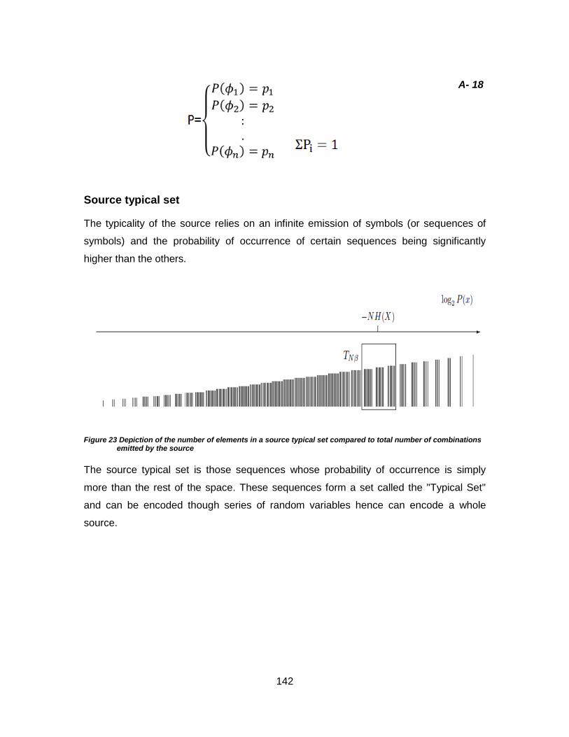
142

A- 18

Source typical set

The typicality of the source relies on an infinite emission of symbols (or sequences of

symbols) and the probability of occurrence of certain sequences being significantly

higher than the others.

Figure 23 Depiction of the number of elements in a source typical set compared to total number of combinations emitted by the source

The source typical set is those sequences whose probability of occurrence is simply

more than the rest of the space. These sequences form a set called the "Typical Set"

and can be encoded though series of random variables hence can encode a whole

source.

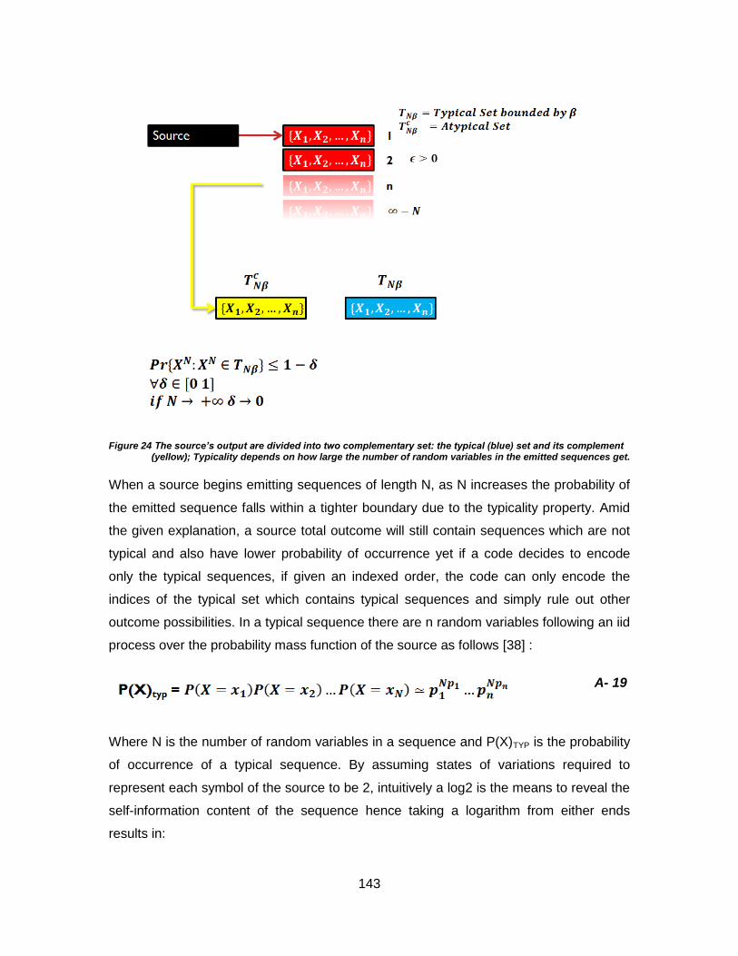
143

Figure 24 The source’s output are divided into two complementary set: the typical (blue) set and its complement (yellow); Typicality depends on how large the number of random variables in the emitted sequences get.

When a source begins emitting sequences of length N, as N increases the probability of

the emitted sequence falls within a tighter boundary due to the typicality property. Amid

the given explanation, a source total outcome will still contain sequences which are not

typical and also have lower probability of occurrence yet if a code decides to encode

only the typical sequences, if given an indexed order, the code can only encode the

indices of the typical set which contains typical sequences and simply rule out other

outcome possibilities. In a typical sequence there are n random variables following an iid

process over the probability mass function of the source as follows [38] :

A- 19

Where N is the number of random variables in a sequence and P(X)TYP is the probability

of occurrence of a typical sequence. By assuming states of variations required to

represent each symbol of the source to be 2, intuitively a log2 is the means to reveal the

self-information content of the sequence hence taking a logarithm from either ends

results in:

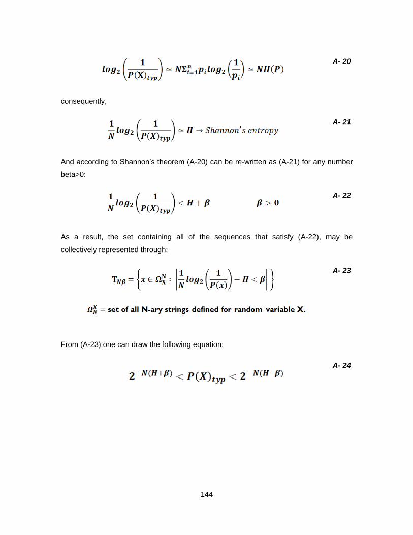
144

A- 20

consequently,

A- 21

And according to Shannon‟s theorem (A-20) can be re-written as (A-21) for any number

beta>0:

A- 22

As a result, the set containing all of the sequences that satisfy (A-22), may be

collectively represented through:

A- 23

From (A-23) one can draw the following equation:

A- 24

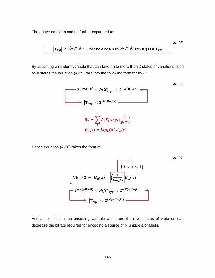
145

The above equation can be further expanded to:

A- 25

By assuming a random variable that can take on to more than 2 states of variations such

as b states the equation (A-25) falls into the following form for b>2 :

A- 26

Hence equation (A-26) takes the form of:

A- 27

And as conclusion, an encoding variable with more than two states of variation can

decrease the bitrate required for encoding a source of N unique alphabets.

146

Appendix II. Grating Angular Dispersion Analysis

For in-plane diffraction, the diffraction grating is described through the grating equation:

A- 28

where parameters alpha and beta are the angles of incidence and diffraction

respectively and m is the order of diffraction along with d being the grating periodicity.

For calculation of how well the grating disperses an incident light or to measure the

grating‟s angular dispersion, with considerations for fixed parameters (here the angle of

incidence) a derivative of (A-28) with respect to the incident wavelength will result in:

A- 29

Where quantity D is dimensionless and deems to show the amount of change of the

diffraction angle between a wavelength and a slightly different one. By replacing the

diffraction angle in (A-29) with (A-28) solved for β, we come across the following (m=1):

147

A- 30

Figure 25 Graphing A-2 3 (6) shows the effect of changes in angle of incidence and wave length as a function of grating periodicity

And further choices for the optimal dispersion (angular dispersion) made clear on the

graphs:

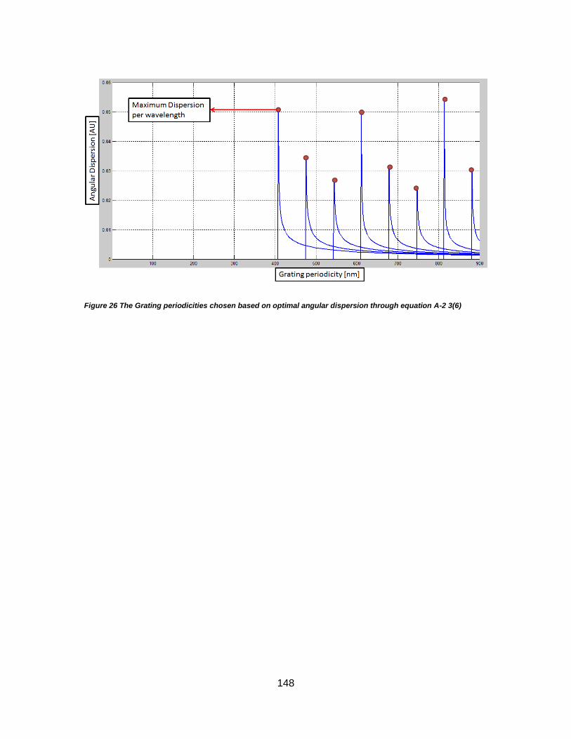
148

Figure 26 The Grating periodicities chosen based on optimal angular dispersion through equation A-2 3(6)

149

Appendix III. Nano-Array Design Software

The array design software performs in the following steps as shown in the block

diagram.

Figure 27 System design block diagram of NOF encoding scheme

Following block diagrams show the general structure of the software algorithm. Due to

publication limits the details of the given block diagram cannot be published. The list of

variables used in the diagram is as follows:

BL=Block Structure

G=Global Variable

COM=Comparison and decision making

MAIN=Main Function

DIR=File Directory

PTH=Path;FNAME=FileName;FBRW=FileBrowse;PrioX=PriorityX;UGTG=Get(file) Commands

O=Output

HDD=Hard Disk(Storage)

150

Figure 28 Nano-Array Design Software Schematic Diagram for Top)-GDSII file header generation and Bottom)-GDSII file main structure generation

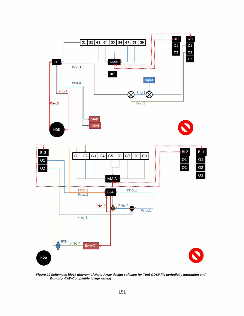
151

Figure 29 Schematic block diagram of Nano-Array design software for Top)-GDSII file periodicity attribution and Bottom)- CAD-Compatible image writing

152

Figure 30 Closed-from schematic block diagram of the Nano-Array design software for generation of CAD-Compatible file formats (GDSII) for EBL Nano-fabrication systems

153

Appendix IV. Overall Comparison of Applied Lossy Compression Algorithms

DCT (Discrete Cosine Transform)

As to the fact that for every compressor module there is a likelihood of a transmission

setup ready to transmit the compressed data, multiple attempts have been made to

decrease the bitrate and consequently modulation bit error rate of a data stream,

outputted from the algorithm and into the transmitting channel. The Discrete cosine

transform has the ability to (similar to wavelet transform) decompose an image into

frequency components being uncorrelated. Frequency correlation or autocorrelation is in

fact a sign of inter-value data redundancies, which in an image, is the main contributor to

the size of the data presented in the output matrix. By applying a DCT to an image

matrix with inter-related data values (entries), one can decompose (de-correlate) the

pixel values into frequency based cosine wave forms which due to the nature of the

transform will get assembled from low to high (base to least). As a known fact in image

processing, human brain is more sensitive towards the low-frequency visual data rather

than high frequencies and also consequently removal of many high frequency

components of the de-correlated image allows for reconstruction of those components

which have the least amount of spatial correlation without losing an overall visual

integrity of the data. The DCT in two-dimensions is calculated through:

A- 31

for x,y=0,1,2,…,N-1

154

Below are the graphs for image compression trials ran through a discrete cosine

transform module and being compared regarding psycho-visual quality, Mean Squared

Error and Peak signal to noise ratio between the original and the compressed image.

Figure 31 Top)- A 2D DCT coefficient matrix with directional DCT-wavelet distribution bottom)-a) An image scanline before(left) and after dct transform(right) b)Autocorrelation diagram of the image scanline before(left) and after dct transform (right);

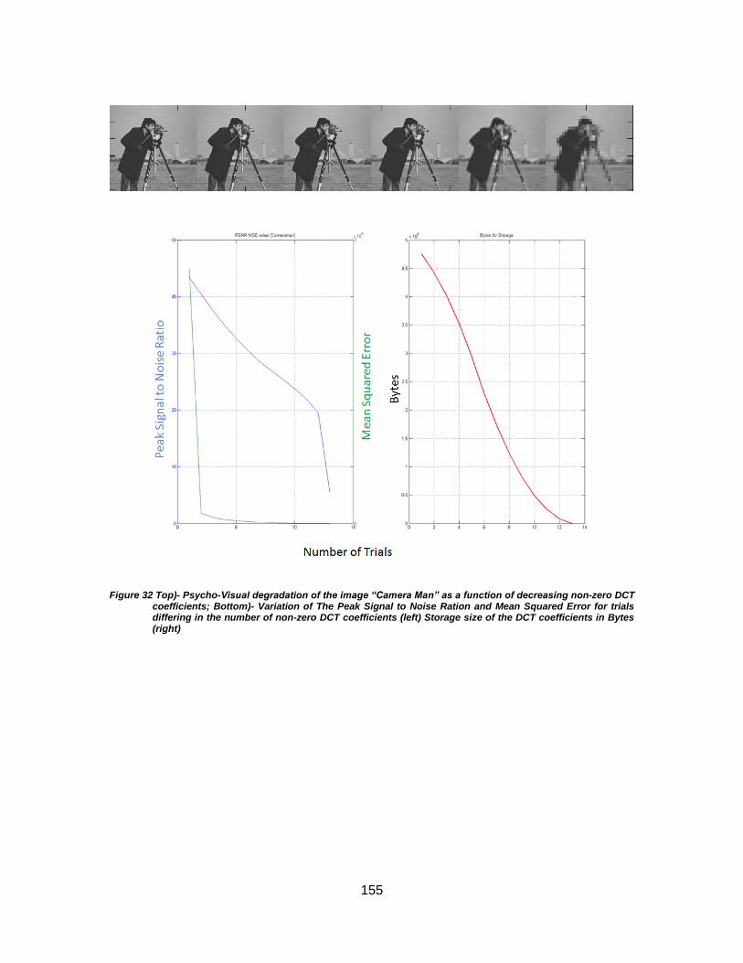
155

Figure 32 Top)- Psycho-Visual degradation of the image “Camera Man” as a function of decreasing non-zero DCT coefficients; Bottom)- Variation of The Peak Signal to Noise Ration and Mean Squared Error for trials differing in the number of non-zero DCT coefficients (left) Storage size of the DCT coefficients in Bytes (right)

156

Figure 33 Top)- Psycho-Visual degradation of the image “Apple” as a function of decreasing non-zero DCT coefficients; Bottom)- Variation of The Peak Signal to Noise Ration and Mean Squared Error for trials differing in the number of non-zero DCT coefficients; (left) Storage size of the DCT coefficients in Bytes (right)

157

Wavelet Transform

The main disadvantage of Fourier Transform is the lack of time lags for a transformed

signal. As to the matter that any signal that has been analyzed through an FFT (Fast

Fourier Transform) module can mainly remain intact or undergo a total loss if the

lowpass of highpass filtering results in loss of visually important yet high energy data in

the image. The most recent mathematical solution to this problem has been the wavelet

transform. In brief a wavelet transform, similar to a Fourier Transform takes the image

(or data) into the frequency domain with the slight difference that what it outputs is

localized both in frequency and time due to an scaling factor that is calculated as a result

of averaging the entries in a particular window and a translation factor that is calculated

due to altering the length of the window that scans the signal. The combination of the

two brings about a collection of temporal frequency scattering of a signal in the wavelet

space. The resulting small functions that interact with each window (interval) of the

signal are called wavelets and they must have certain mathematical characteristics in

order to be invertible. These properties in brief are: 1) Admissibility and 2) Regularity. To

achieve an invertible wavelet transform coefficient matrix one must perform the

admissibility check which imposes that the Fourier transform of the signal must be zero

at zero frequency.

A- 32

Where γ(S,T) is the wavelet transform of the data, ψST is the wavelet notion and S, T are

Scaling and Translation of the signal.

A- 33

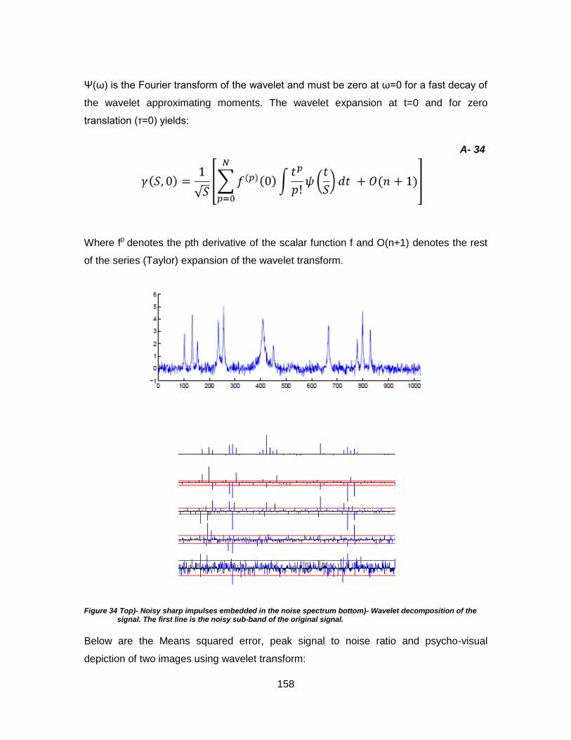
158

Ψ(ω) is the Fourier transform of the wavelet and must be zero at ω=0 for a fast decay of

the wavelet approximating moments. The wavelet expansion at t=0 and for zero

translation (τ=0) yields:

A- 34

Where fp denotes the pth derivative of the scalar function f and O(n+1) denotes the rest

of the series (Taylor) expansion of the wavelet transform.

Figure 34 Top)- Noisy sharp impulses embedded in the noise spectrum bottom)- Wavelet decomposition of the signal. The first line is the noisy sub-band of the original signal.

Below are the Means squared error, peak signal to noise ratio and psycho-visual

depiction of two images using wavelet transform:

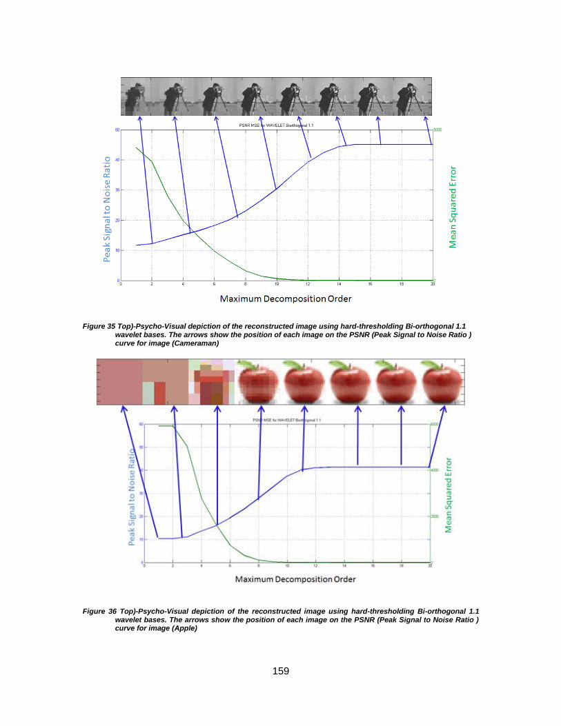
159

Figure 35 Top)-Psycho-Visual depiction of the reconstructed image using hard-thresholding Bi-orthogonal 1.1 wavelet bases. The arrows show the position of each image on the PSNR (Peak Signal to Noise Ratio ) curve for image (Cameraman)

Figure 36 Top)-Psycho-Visual depiction of the reconstructed image using hard-thresholding Bi-orthogonal 1.1 wavelet bases. The arrows show the position of each image on the PSNR (Peak Signal to Noise Ratio ) curve for image (Apple)

160

Appendix V. Deriving A Complex Angle of Incidence for Angular Dispersion

There could be assumed a special case where the changes of dispersion quantity relies

only and only on the incident wavelength and the grating periodicity with the angle of

diffraction effect being suppressed, this happens under certain conditions for the choice

of the incidence angle in which the value chosen becomes complex. The graph in Figure

37 shows an investigation of the aforementioned conditions.

Figure 37 Effect of a complex angle of incidence on the angular resolution (dispersion power) of the grating

This condition is produced through transformation of (A-2 3) into the following equation:

A- 35

The condition for producing a complex angle of incidence requires complex analysis of

the incidence medium and due to presence of a phase (imaginary component) in the

equation; one must define physical properties with multiple layer structure and different

indices of refraction to achieve a complex angle of incidence. We denote the advantage

of using what shown in Figure 37 is a more controllable partial change for the angular

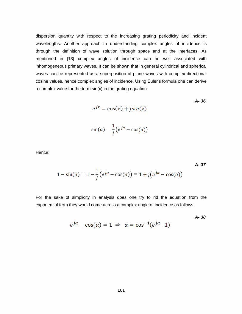
161

dispersion quantity with respect to the increasing grating periodicity and incident

wavelengths. Another approach to understanding complex angles of incidence is

through the definition of wave solution through space and at the interfaces. As

mentioned in [13] complex angles of incidence can be well associated with

inhomogeneous primary waves. It can be shown that in general cylindrical and spherical

waves can be represented as a superposition of plane waves with complex directional

cosine values, hence complex angles of incidence. Using Euler‟s formula one can derive

a complex value for the term sin(x) in the grating equation:

A- 36

Hence:

A- 37

For the sake of simplicity in analysis does one try to rid the equation from the

exponential term they would come across a complex angle of incidence as follows:

A- 38

162

Figure 38. Contour diagrams showing the real and imaginary field distribution of a grating with complex angles of incidence.

In theory such angle of incidence gives rise to a complex field distribution which its

physical interpretation and implementation is outside the scope of the current work.

163

Appendix VI. Encoding Definition via Set Theory and Boolean Logic

The fundamentals of digital data encoding are not that different from the mathematical

definition of bijective functions. The mentioned methods in 2.3 transfer the values of the

input data from the analog domain into the binary frame of digital domain. Such

transform, assigns a binary value to the measured signal sample at the input of the

encoder. This transform before being perceived by the machine logic, is usually a

voltage or current measurement which is considered to be a continuous real-valued

sampling which also stores the quantified continuous value of the real signal within a

discrete storage medium. The dimensions of the stored signal (data segment) are (due

to Nyquist Sampling Theorem) less than dimension of the real-valued data unless the

data itself is in discrete values. The key target of this section is to prove through

mathematical derivation that for discrete numerical values it is possible to reduce the

number of digital domain unit data carriers through use of higher states of variation for a

single digital information unit. We will begin the investigation by having two sets which

represent the original and the encoded data respectively. In this example we choose the

original set of information to contain quantifications or numerical values which historically

tend to be universal among all systems. The set X is the set of all positive integers. This

set can be labeled as the upper half of the natural numbers including the quantity for

non-existent zero. We argue that if a system tends to encode this original set into a

secondary or target set Y, this mapping should allow for existence of equivalent number

of encoders hence both the original set and the encoded set have same number of

elements or same cardinality. This proof shows that what does it mean to encode a set

of data through logical and mathematical approaches with the goal of using the proof to

argue benefits of the presented work. Any storage of data is a mathematical concept that

can be best described through the set theory. The depiction of the data set to be stored

and the stored data set can in general form take the analogy of two sets X and Y

respectively where all elements of X are mapped onto the elements of set Y through

function f. in order for f to satisfy mapping conditions there are four preconditions to be

met:

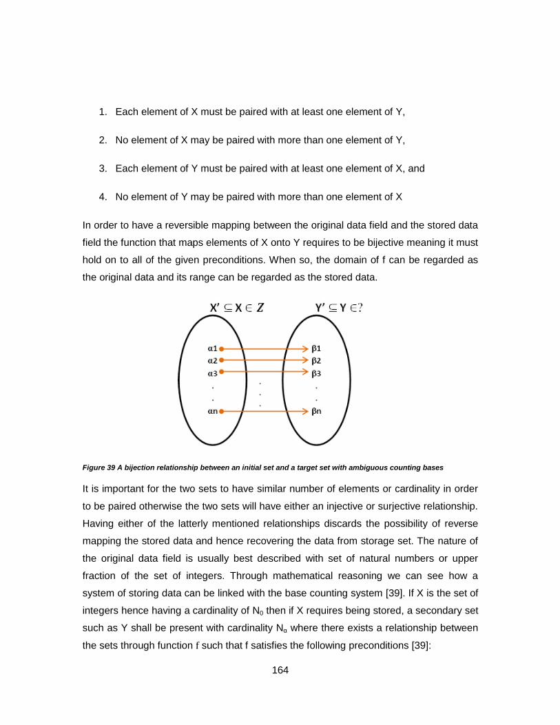
164

1. Each element of X must be paired with at least one element of Y,

2. No element of X may be paired with more than one element of Y,

3. Each element of Y must be paired with at least one element of X, and

4. No element of Y may be paired with more than one element of X

In order to have a reversible mapping between the original data field and the stored data

field the function that maps elements of X onto Y requires to be bijective meaning it must

hold on to all of the given preconditions. When so, the domain of f can be regarded as

the original data and its range can be regarded as the stored data.

Figure 39 A bijection relationship between an initial set and a target set with ambiguous counting bases

It is important for the two sets to have similar number of elements or cardinality in order

to be paired otherwise the two sets will have either an injective or surjective relationship.

Having either of the latterly mentioned relationships discards the possibility of reverse

mapping the stored data and hence recovering the data from storage set. The nature of

the original data field is usually best described with set of natural numbers or upper

fraction of the set of integers. Through mathematical reasoning we can see how a

system of storing data can be linked with the base counting system [39]. If X is the set of

integers hence having a cardinality of N0 then if X requires being stored, a secondary set

such as Y shall be present with cardinality Nα where there exists a relationship between

the sets through function f such that f satisfies the following preconditions [39]:

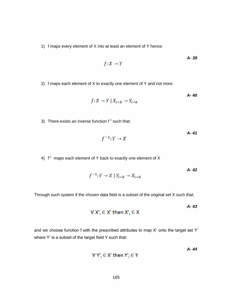
165

1) f maps every element of X into at least an element of Y hence:

A- 39

2) f maps each element of X to exactly one element of Y and not more

A- 40

3) There exists an inverse function f-1 such that:

A- 41

4) f-1 maps each element of Y back to exactly one element of X

A- 42

Through such system if the chosen data field is a subset of the original set X such that:

A- 43

and we choose function f with the prescribed attributes to map X‟ onto the target set Y‟

where Y‟ is a subset of the target field Y such that:

A- 44

166

(A-44) clearly indicates that cardinality N (number of elements of the sets) must be equal

and this means that there must be equivalent amount of elements within both sets in

order for f to be able to map them back and forth [39]. The computer sciences model the

unit information carrier as one bit which is also in a Boolean logic framework. There are

quantities of unit information carriers in a machine arithmetic model where each

transition between variables follows a true/false state and as a result each function that

receives and transmits a single state of true or false also is a Boolean function. The

particularity of Boolean algebra is based on having full arithmetic qualities alongside its

bi-state initial set. The aforementioned property of Boolean algebra and Boolean

functions makes its arithmetic space (set of all bi-element sets and all functions

operating on them) a suitable space for storing information using only two elements of a

given set. Because a logic set having only two distinct possibilities (e.g. true or false) is

easy to replicate in a physical sense (e.g. on/off, current/no current, voltage / no voltage)

it seems intuitive for function f mentioned in (A-39) through (A-44) to be a Boolean

function [39]. For understanding the significance of Boolean nature of function f it is also

necessary to understand the representation of numbers in the set of data to be stored X‟.

X‟ is a subset of X which in our analysis is the set of upper fraction of the integers and

has an infinite cardinality N0. The mathematical representation of any element of X‟ will

have the general form [39]:

A- 45

167

If di is considered to expand the numerals to an unknown base b then :

A- 46

And the largest n-digit number to be represented by this system is:

A- 47

As to the fact that physical representation of elements of the target set Y‟ are chosen to

be of bi-element nature (Belonging to the set {0,1} ) and having the constraint of bijection

for any function f that maps between the two sets, each element of X‟ and Y‟ shall have

a relationship where [39] :

A- 48

The relationship between α and β can be found through modular arithmetic [39]:

A- 49

Sets A_bar and B_bar are the congruent classes of elements αi and βi where depending

on the divisor b and b_hat, the number of unique elements to be represented will be

defined. Hence for set X‟ b=10 and if the goal is to have a logical function to act on αi

then b_hat=2. f will have to act on a Boolean domain whereas the set X‟ is not a Boolean

domain. f requires then to be first acting on the Natural domain and next on a logical

(Boolean) domain:

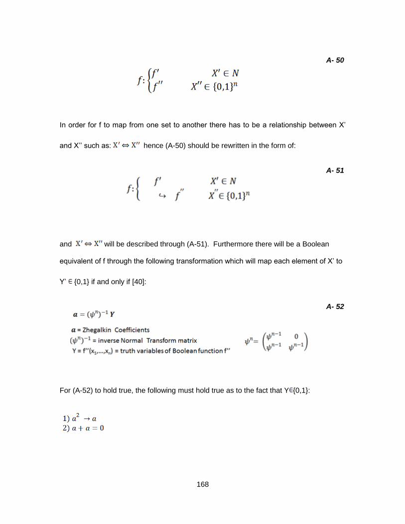
168

A- 50

In order for f to map from one set to another there has to be a relationship between X‟

and X‟‟ such as: hence (A-50) should be rewritten in the form of:

A- 51

and will be described through (A-51). Furthermore there will be a Boolean

equivalent of f through the following transformation which will map each element of X‟ to

Y‟ {0,1} if and only if [40]:

A- 52

For (A-52) to hold true, the following must hold true as to the fact that Y {0,1}:

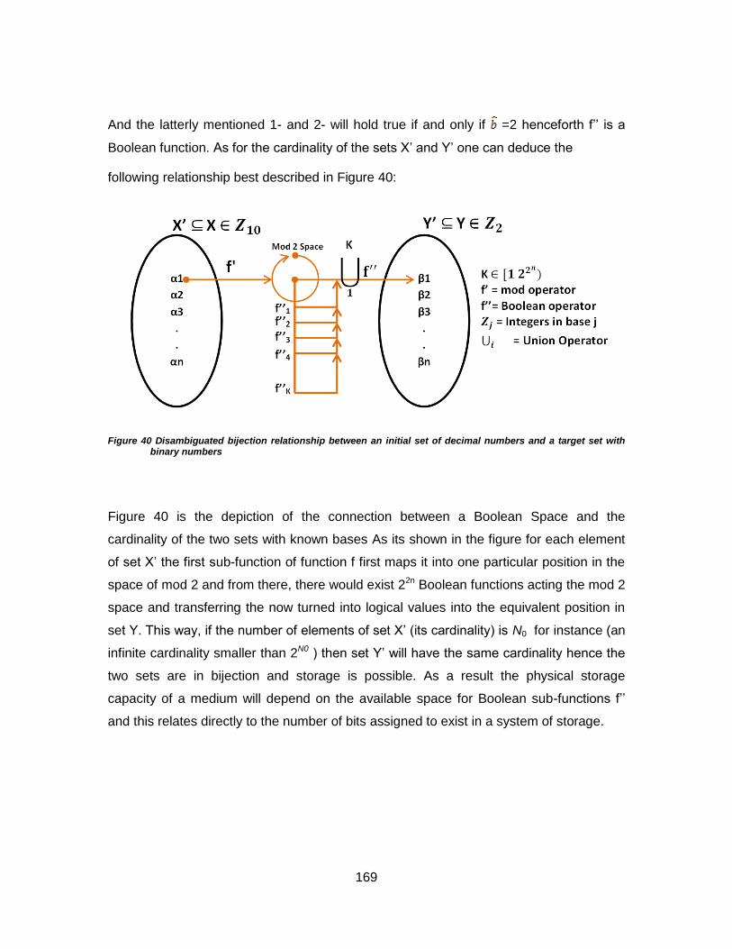
169

And the latterly mentioned 1- and 2- will hold true if and only if =2 henceforth f‟‟ is a

Boolean function. As for the cardinality of the sets X‟ and Y‟ one can deduce the

following relationship best described in Figure 40:

Figure 40 Disambiguated bijection relationship between an initial set of decimal numbers and a target set with binary numbers

Figure 40 is the depiction of the connection between a Boolean Space and the

cardinality of the two sets with known bases As its shown in the figure for each element

of set X‟ the first sub-function of function f first maps it into one particular position in the

space of mod 2 and from there, there would exist 22n Boolean functions acting the mod 2

space and transferring the now turned into logical values into the equivalent position in

set Y. This way, if the number of elements of set X‟ (its cardinality) is N0 for instance (an

infinite cardinality smaller than 2N0 ) then set Y‟ will have the same cardinality hence the

two sets are in bijection and storage is possible. As a result the physical storage

capacity of a medium will depend on the available space for Boolean sub-functions f‟‟

and this relates directly to the number of bits assigned to exist in a system of storage.