Articleshttps://doi.org/10.1038/s41560-019-0356-8

1Department of Chemical Engineering, Massachusetts Institute of Technology, Cambridge, MA, USA. 2Department of Materials Science and Engineering, Stanford University, Stanford, CA, USA. 3Toyota Research Institute, Los Altos, CA, USA. 4Materials Science Division, Lawrence Berkeley National Lab, Berkeley, CA, USA. 5These authors contributed equally: K. A. Severson, P. M. Attia. *e-mail: wchueh@stanford.edu; braatz@mit.edu

Lithium-ion batteries are deployed in a wide range of applica-tions due to their low and falling costs, high energy densities and long lifetimes1–3. However, as is the case with many chemi-

cal, mechanical and electronic systems, long battery lifetime entails delayed feedback of performance, often many months to years. Accurate prediction of lifetime using early-cycle data would unlock new opportunities in battery production, use and optimization. For example, manufacturers can accelerate the cell development cycle, perform rapid validation of new manufacturing processes and sort/grade new cells by their expected lifetime. Likewise, end users could estimate their battery life expectancy4–6. One emerging application enabled by early prediction is high-throughput optimization of processes spanning large parameter spaces (Supplementary Figs. 1 and 2), such as multistep fast charging and formation cycling, which are otherwise intractable due to the extraordinary time required. The task of predicting lithium-ion battery lifetime is critically important given its broad utility but challenging due to nonlinear degradation with cycling and wide variability, even when control-ling for operating conditions7–11.

Many previous studies have modelled lithium-ion battery life-time. Bloom et al.12 and Broussely et al.13 performed early work that fitted semi-empirical models to predict power and capacity loss. Since then, many authors have proposed physical and semi-empir-ical models that account for diverse mechanisms such as growth of the solid–electrolyte interphase14,15, lithium plating16,17, active mate-rial loss18,19 and impedance increase20–22. Predictions of remaining useful life in battery management systems, summarized in these reviews5,6, often rely on these mechanistic and semi-empirical mod-els for state estimation. Specialized diagnostic measurements such as coulombic efficiency23,24 and impedance spectroscopy25–27 can also be used for lifetime estimation. While these chemistry and/or mechanism-specific models have shown predictive success, devel-oping models that describe full cells cycled under relevant operating

conditions (for example, fast charging) remains challenging, given the many degradation modes and their coupling to thermal28,29 and mechanical28,30 heterogeneities within a cell30–32.

Approaches using statistical and machine-learning techniques to predict cycle life are attractive, mechanism-agnostic alternatives. Recently, advances in computational power and data generation have enabled these techniques to accelerate progress for a variety of tasks, including prediction of material properties33,34, identifica-tion of chemical synthesis routes35 and material discovery for energy storage36–38 and catalysis39. A growing body of literature6,40,41 applies machine-learning techniques for predicting the remaining useful life of batteries using data collected in both laboratory and online environments. Generally, these works make predictions after accu-mulating data corresponding to degradation of at least 25% along the trajectory to failure42–48 or using specialized measurements at the beginning of life11. Accurate early prediction of cycle life with significantly less degradation is challenging because of the typically nonlinear degradation process (with negligible capacity degrada-tion in early cycles) as well as the relatively small datasets used to date that span a limited range of lifetimes49. For example, Harris et al.10 found a weak correlation (ρ = 0.1) between capacity values at cycle 80 and capacity values at cycle 500 for 24 cells exhibiting nonlinear degradation profiles, illustrating the difficulty of this task. Machine-learning approaches are especially attractive for high-rate operating conditions, where first-principles models of degradation are often unavailable. In short, opportunities for improving upon state-of-the-art prediction models include higher accuracy, earlier prediction, greater interpretability and broader application to a wide range of cycling conditions.

In this work, we develop data-driven models that accurately predict the cycle life of commercial lithium iron phosphate (LFP)/graphite cells using early-cycle data, with no prior knowledge of degradation mechanisms. We generated a dataset of 124 cells with

Data-driven prediction of battery cycle life before capacity degradationKristen A. Severson   1,5, Peter M. Attia   2,5, Norman Jin   2, Nicholas Perkins   2, Benben Jiang   1, Zi Yang   2, Michael H. Chen   2, Muratahan Aykol   3, Patrick K. Herring   3, Dimitrios Fraggedakis   1, Martin Z. Bazant   1, Stephen J. Harris   2,4, William C. Chueh   2* and Richard D. Braatz   1*

Accurately predicting the lifetime of complex, nonlinear systems such as lithium-ion batteries is critical for accelerating tech-nology development. However, diverse aging mechanisms, significant device variability and dynamic operating conditions have remained major challenges. We generate a comprehensive dataset consisting of 124 commercial lithium iron phosphate/graphite cells cycled under fast-charging conditions, with widely varying cycle lives ranging from 150 to 2,300 cycles. Using discharge voltage curves from early cycles yet to exhibit capacity degradation, we apply machine-learning tools to both predict and classify cells by cycle life. Our best models achieve 9.1% test error for quantitatively predicting cycle life using the first 100 cycles (exhibiting a median increase of 0.2% from initial capacity) and 4.9% test error using the first 5 cycles for classifying cycle life into two groups. This work highlights the promise of combining deliberate data generation with data-driven modelling to predict the behaviour of complex dynamical systems.

NAtuRe eNeRgY | www.nature.com/natureenergy

Articles NATUre eNergy

cycle lives ranging from 150 to 2,300 using 72 different fast-charg-ing conditions, with cycle life (or equivalently, end of life) defined as the number of cycles until 80% of nominal capacity. For quanti-tatively predicting cycle life, our feature-based models can achieve prediction errors of 9.1% using only data from the first 100 cycles, at which point most batteries have yet to exhibit capacity degradation. Furthermore, using data from the first 5 cycles, we demonstrate classification into low- and high-lifetime groups and achieve a mis-classification test error of 4.9%. These results illustrate the power of combining data generation with data-driven modelling to predict the behaviour of complex systems far into the future.

Data generationWe expect the space that parameterizes capacity fade in lithium-ion batteries to be high dimensional due to their many capac-ity fade mechanisms and manufacturing variability. To probe this space, commercial LFP/graphite cells (A123 Systems, model

APR18650M1A, 1.1 Ah nominal capacity) were cycled in a tem-perature-controlled environmental chamber (30 °C) under var-ied fast-charging conditions but identical discharging conditions (4 C to 2.0 V, where 1 C is 1.1 A; see Methods for details). Since the graphite negative electrode dominates degradation in these cells, these results could be useful for other lithium-ion batteries based on graphite32,50–54. We probe average charging rates ranging from 3.6 C, the manufacturer’s recommended fast-charging rate, to 6 C to probe the performance of current-generation power cells under extreme fast-charging conditions (~10 min charging), an area of significant commercial interest55. By deliberately varying the charg-ing conditions, we generate a dataset that captures a wide range of cycle lives, from approximately 150 to 2,300 cycles (average cycle life of 806 with a standard deviation of 377). While the chamber temperature is controlled, the cell temperatures vary by up to 10 °C within a cycle due to the large amount of heat generated during charge and discharge. This temperature variation is a function of

0 100 200 300 400 500 600 700 800 900 1,000

Cycle number

0.90

0.95

1.00

1.05

1.10

Dis

char

ge c

apac

ity (

Ah)

20 40 60 80 100

Cycle number

1.00

1.05

1.10

Dis

char

ge c

apac

ity (

Ah)

1 1.1

Discharge capacityat cycle 2 (Ah)

102

103

102

103

102

103

Cyc

le li

fe

Cyc

le li

fe

Cyc

le li

fe

1 1.1

Discharge capacityat cycle 100 (Ah)

–2 –1 0

Slope of discharge capacity cycles 95–100 (mAh per cycle)

0.96 0.98 1.00 1.02

Capacity ratio, cycles 100:2

0

50

100

Cou

nt

0

a

b

d e f

c

ρ = –0.061 ρ = 0.27 ρ = 0.47

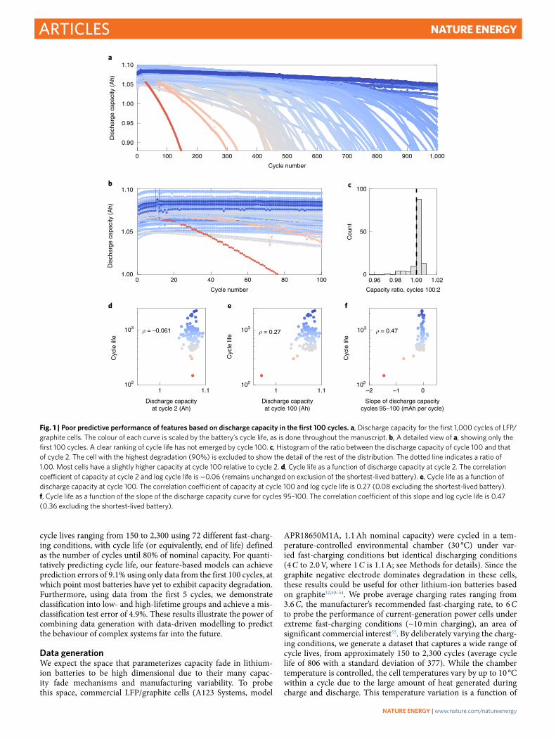
Fig. 1 | Poor predictive performance of features based on discharge capacity in the first 100 cycles. a, Discharge capacity for the first 1,000 cycles of LFP/graphite cells. The colour of each curve is scaled by the battery’s cycle life, as is done throughout the manuscript. b, A detailed view of a, showing only the first 100 cycles. A clear ranking of cycle life has not emerged by cycle 100. c, Histogram of the ratio between the discharge capacity of cycle 100 and that of cycle 2. The cell with the highest degradation (90%) is excluded to show the detail of the rest of the distribution. The dotted line indicates a ratio of 1.00. Most cells have a slightly higher capacity at cycle 100 relative to cycle 2. d, Cycle life as a function of discharge capacity at cycle 2. The correlation coefficient of capacity at cycle 2 and log cycle life is −0.06 (remains unchanged on exclusion of the shortest-lived battery). e, Cycle life as a function of discharge capacity at cycle 100. The correlation coefficient of capacity at cycle 100 and log cycle life is 0.27 (0.08 excluding the shortest-lived battery). f, Cycle life as a function of the slope of the discharge capacity curve for cycles 95–100. The correlation coefficient of this slope and log cycle life is 0.47 (0.36 excluding the shortest-lived battery).

NAtuRe eNeRgY | www.nature.com/natureenergy

ArticlesNATUre eNergy

internal impedance and charging policy (Supplementary Figs. 3 and 4). Voltage, current, cell can temperature and internal resis-tance are continuously measured during cycling (see Methods for additional experimental details). The dataset contains approxi-mately 96,700 cycles; to the best of the authors’ knowledge, our dataset is the largest publicly available for nominally identical com-mercial lithium-ion batteries cycled under controlled conditions (see Data availability section for access information).

Fig. 1a,b shows the discharge capacity as a function of cycle number for the first 1,000 cycles, where the colour denotes cycle life. The capacity fade is negligible in the first 100 cycles and accel-erates near the end of life, as is often observed in lithium-ion bat-teries. The crossing of the capacity fade trajectories illustrates the weak relationship between initial capacity and lifetime; indeed, we find weak correlations between the log of cycle life and the discharge capacity at the second cycle (ρ = −0.06, Fig. 1d) and the 100th cycle (ρ = 0.27, Fig. 1e), as well as between the log of cycle life and the capacity fade rate near cycle 100 (ρ = 0.47, Fig. 1f). These weak correlations are expected because capacity degrada-tion in these early cycles is negligible; in fact, the capacities at cycle 100 increased from the initial values for 81% of cells in our dataset (Fig. 1c). Small increases in capacity after a slow cycle or rest period are attributed to charge stored in the region of the negative elec-trode that extends beyond the positive electrode56,57. Given the lim-ited predictive power of these correlations based on the capacity

fade curves, we employ an alternative data-driven approach that considers a larger set of cycling data including the full voltage curves of each cycle, as well as additional measurements including cell internal resistance and temperature.

Machine-learning approachWe use a feature-based approach to build an early-prediction model. In this paradigm, features, which are linear or nonlinear transforma-tions of the raw data, are generated and used in a regularized linear framework, the elastic net58. The final model uses a linear combina-tion of a subset of the proposed features to predict the logarithm of cycle life. Our choice of a regularized linear model allows us to propose domain-specific features of varying complexity while main-taining high interpretability. Linear models also have low computa-tional cost; the model can be trained offline, and online prediction requires only a single dot product after data preprocessing.

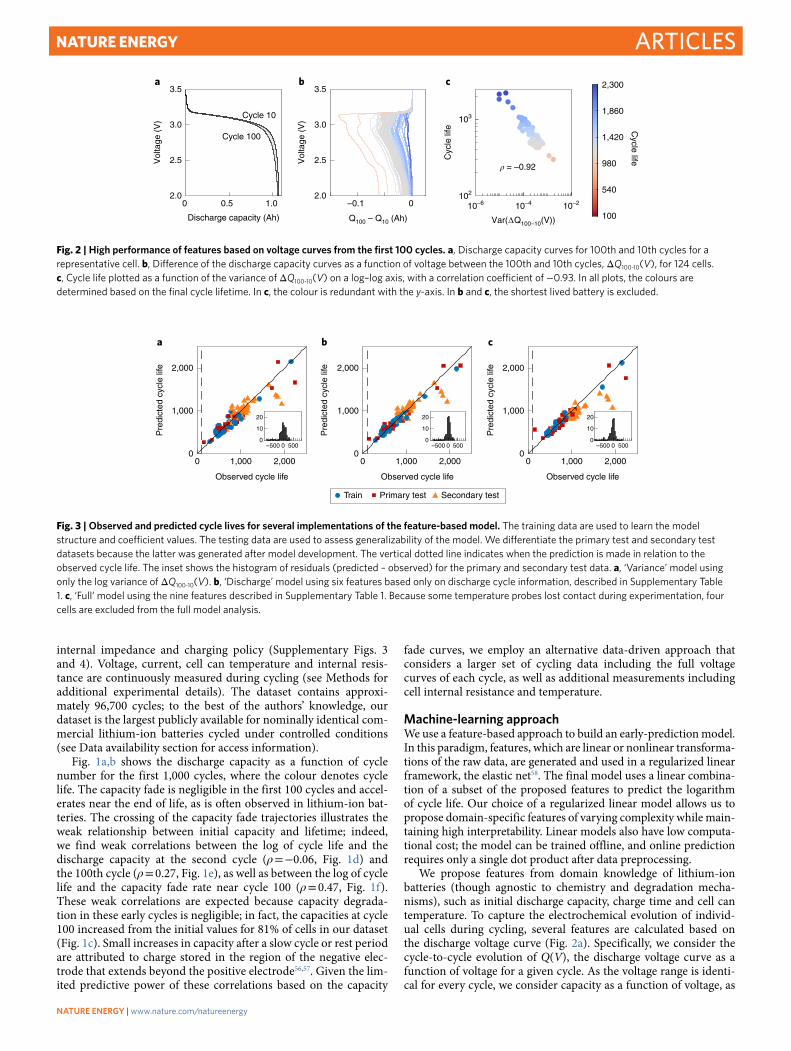
We propose features from domain knowledge of lithium-ion batteries (though agnostic to chemistry and degradation mecha-nisms), such as initial discharge capacity, charge time and cell can temperature. To capture the electrochemical evolution of individ-ual cells during cycling, several features are calculated based on the discharge voltage curve (Fig. 2a). Specifically, we consider the cycle-to-cycle evolution of Q(V), the discharge voltage curve as a function of voltage for a given cycle. As the voltage range is identi-cal for every cycle, we consider capacity as a function of voltage, as

10–6 10–4 10–2

Var(∆Q100–10(V))

102

103

Cyc

le li

fe

ρ = –0.92

c

100

540

980

1,420

1,860

2,300

Cycle life

–0.1 0

Q100 – Q10 (Ah)

2.0

2.5

3.0

3.5

Vol

tage

(V

)

b

0 0.5 1.0

Discharge capacity (Ah)

2.0

2.5

3.0

3.5

Vol

tage

(V

)

Cycle 10

Cycle 100

a

Fig. 2 | High performance of features based on voltage curves from the first 100 cycles. a, Discharge capacity curves for 100th and 10th cycles for a representative cell. b, Difference of the discharge capacity curves as a function of voltage between the 100th and 10th cycles, ΔQ100-10(V), for 124 cells. c, Cycle life plotted as a function of the variance of ΔQ100-10(V) on a log–log axis, with a correlation coefficient of −0.93. In all plots, the colours are determined based on the final cycle lifetime. In c, the colour is redundant with the y-axis. In b and c, the shortest lived battery is excluded.

2,000

1,000

2,000

1,000

0 0

2,000

1,000

00 1,000 2,000 0 1,000 2,000 0 1,000 2,000

Observed cycle life Observed cycle life Observed cycle life

Pre

dict

ed c

ycle

life

Pre

dict

ed c

ycle

life

Pre

dict

ed c

ycle

life

20

10

0

20

10

0

20

10

0–500 0 500 –500 0 500 –500 0 500

Train Primary test Secondary test

a b c

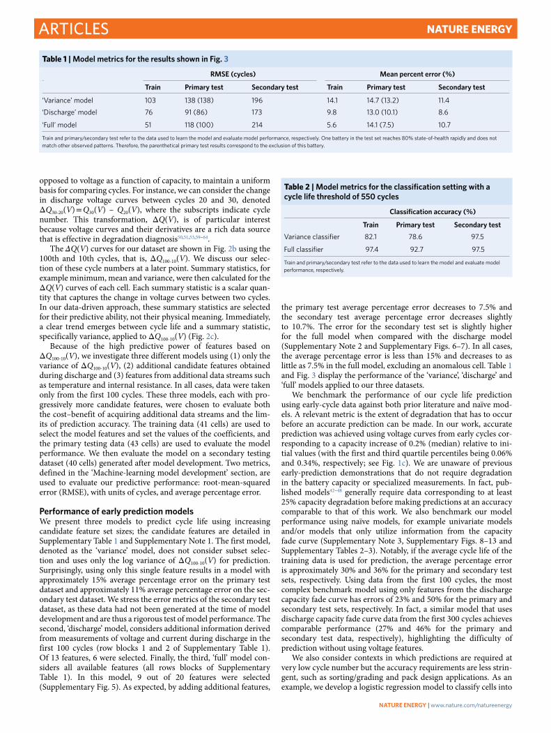
Fig. 3 | Observed and predicted cycle lives for several implementations of the feature-based model. The training data are used to learn the model structure and coefficient values. The testing data are used to assess generalizability of the model. We differentiate the primary test and secondary test datasets because the latter was generated after model development. The vertical dotted line indicates when the prediction is made in relation to the observed cycle life. The inset shows the histogram of residuals (predicted – observed) for the primary and secondary test data. a, ‘Variance’ model using only the log variance of ΔQ100-10(V). b, ‘Discharge’ model using six features based only on discharge cycle information, described in Supplementary Table 1. c, ‘Full’ model using the nine features described in Supplementary Table 1. Because some temperature probes lost contact during experimentation, four cells are excluded from the full model analysis.

NAtuRe eNeRgY | www.nature.com/natureenergy

Articles NATUre eNergy

opposed to voltage as a function of capacity, to maintain a uniform basis for comparing cycles. For instance, we can consider the change in discharge voltage curves between cycles 20 and 30, denoted ΔQ30-20(V) = Q30(V) – Q20(V), where the subscripts indicate cycle number. This transformation, ΔQ(V), is of particular interest because voltage curves and their derivatives are a rich data source that is effective in degradation diagnosis50,51,53,59–64.

The ΔQ(V) curves for our dataset are shown in Fig. 2b using the 100th and 10th cycles, that is, ΔQ100-10(V). We discuss our selec-tion of these cycle numbers at a later point. Summary statistics, for example minimum, mean and variance, were then calculated for the ΔQ(V) curves of each cell. Each summary statistic is a scalar quan-tity that captures the change in voltage curves between two cycles. In our data-driven approach, these summary statistics are selected for their predictive ability, not their physical meaning. Immediately, a clear trend emerges between cycle life and a summary statistic, specifically variance, applied to ΔQ100-10(V) (Fig. 2c).

Because of the high predictive power of features based on ΔQ100-10(V), we investigate three different models using (1) only the variance of ΔQ100-10(V), (2) additional candidate features obtained during discharge and (3) features from additional data streams such as temperature and internal resistance. In all cases, data were taken only from the first 100 cycles. These three models, each with pro-gressively more candidate features, were chosen to evaluate both the cost–benefit of acquiring additional data streams and the lim-its of prediction accuracy. The training data (41 cells) are used to select the model features and set the values of the coefficients, and the primary testing data (43 cells) are used to evaluate the model performance. We then evaluate the model on a secondary testing dataset (40 cells) generated after model development. Two metrics, defined in the ‘Machine-learning model development’ section, are used to evaluate our predictive performance: root-mean-squared error (RMSE), with units of cycles, and average percentage error.

Performance of early prediction modelsWe present three models to predict cycle life using increasing candidate feature set sizes; the candidate features are detailed in Supplementary Table 1 and Supplementary Note 1. The first model, denoted as the ‘variance’ model, does not consider subset selec-tion and uses only the log variance of ΔQ100-10(V) for prediction. Surprisingly, using only this single feature results in a model with approximately 15% average percentage error on the primary test dataset and approximately 11% average percentage error on the sec-ondary test dataset. We stress the error metrics of the secondary test dataset, as these data had not been generated at the time of model development and are thus a rigorous test of model performance. The second, ‘discharge’ model, considers additional information derived from measurements of voltage and current during discharge in the first 100 cycles (row blocks 1 and 2 of Supplementary Table 1). Of 13 features, 6 were selected. Finally, the third, ‘full’ model con-si ders all available features (all rows blocks of Supplementary Table 1). In this model, 9 out of 20 features were selected (Supplementary Fig. 5). As expected, by adding additional features,

the primary test average percentage error decreases to 7.5% and the secondary test average percentage error decreases slightly to 10.7%. The error for the secondary test set is slightly higher for the full model when compared with the discharge model (Supplementary Note 2 and Supplementary Figs. 6–7). In all cases, the average percentage error is less than 15% and decreases to as little as 7.5% in the full model, excluding an anomalous cell. Table 1 and Fig. 3 display the performance of the ‘variance’, ‘discharge’ and ‘full’ models applied to our three datasets.

We benchmark the performance of our cycle life prediction using early-cycle data against both prior literature and naïve mod-els. A relevant metric is the extent of degradation that has to occur before an accurate prediction can be made. In our work, accurate prediction was achieved using voltage curves from early cycles cor-responding to a capacity increase of 0.2% (median) relative to ini-tial values (with the first and third quartile percentiles being 0.06% and 0.34%, respectively; see Fig. 1c). We are unaware of previous early-prediction demonstrations that do not require degradation in the battery capacity or specialized measurements. In fact, pub-lished models42–48 generally require data corresponding to at least 25% capacity degradation before making predictions at an accuracy comparable to that of this work. We also benchmark our model performance using naïve models, for example univariate models and/or models that only utilize information from the capacity fade curve (Supplementary Note 3, Supplementary Figs. 8–13 and Supplementary Tables 2–3). Notably, if the average cycle life of the training data is used for prediction, the average percentage error is approximately 30% and 36% for the primary and secondary test sets, respectively. Using data from the first 100 cycles, the most complex benchmark model using only features from the discharge capacity fade curve has errors of 23% and 50% for the primary and secondary test sets, respectively. In fact, a similar model that uses discharge capacity fade curve data from the first 300 cycles achieves comparable performance (27% and 46% for the primary and secondary test data, respectively), highlighting the difficulty of prediction without using voltage features.

We also consider contexts in which predictions are required at very low cycle number but the accuracy requirements are less strin-gent, such as sorting/grading and pack design applications. As an example, we develop a logistic regression model to classify cells into

Table 1 | Model metrics for the results shown in Fig. 3

RMSe (cycles) Mean percent error (%)

train Primary test Secondary test train Primary test Secondary test

‘Variance’ model 103 138 (138) 196 14.1 14.7 (13.2) 11.4

‘Discharge’ model 76 91 (86) 173 9.8 13.0 (10.1) 8.6

‘Full’ model 51 118 (100) 214 5.6 14.1 (7.5) 10.7

Train and primary/secondary test refer to the data used to learn the model and evaluate model performance, respectively. One battery in the test set reaches 80% state-of-health rapidly and does not match other observed patterns. Therefore, the parenthetical primary test results correspond to the exclusion of this battery.

Table 2 | Model metrics for the classification setting with a cycle life threshold of 550 cycles

Classification accuracy (%)

train Primary test Secondary testVariance classifier 82.1 78.6 97.5

Full classifier 97.4 92.7 97.5

Train and primary/secondary test refer to the data used to learn the model and evaluate model performance, respectively.

NAtuRe eNeRgY | www.nature.com/natureenergy

ArticlesNATUre eNergy

either a ‘low-lifetime’ or a ‘high-lifetime’ group, using only the first five cycles for various cycle life thresholds. For the ‘variance clas-sifier’, we use only the ΔQ(V) variance feature between the fourth and fifth cycles, var(ΔQ5-4(V)), and attain a test classification accu-racy of 88.8%. For the ‘full classifier’, we use regularized logistic regression with 18 candidate features to achieve a test classification accuracy of 95.1%. These results are summarized in Table 2 and detailed in Supplementary Note 4, Supplementary Fig. 14–17 and Supplementary Tables 4–6. This approach illustrates the predictive ability of ΔQ(V) even if data from the only first few cycles are used, and, more broadly, showcases our flexibility to tailor data-driven models to various use cases.

Rationalization of predictive performanceWhile models that include features from all available data streams generally have the lowest errors, our predictive ability primary comes from features based on transformations of the voltage curves, as evidenced by the performance of the single-feature ‘variance’ model. This feature is consistently selected in both models with fea-ture selection (‘discharge’ and ‘full’). Other transformations of the voltage curves can also be used to predict cycle life; for example, the full model selects both the minimum and variance of ΔQ100-10(V). In particular, the physical meaning of the variance feature is associ-ated with the dependence of the discharged energy dissipation on voltage, which is indicated by the grey region between the voltage

0

–10

–20

–30

0

–10

–20

–30

0

–10

–20

–30

3.2 3.3 3.4 3.2 3.3 3.4 3.2 3.3 3.4

C/10 C/10 C/10

C/10C/10C/10

4 C 4 C 4 C

4 C4 C4 C

d%Q

/dV

(%

V−

1 )dV

/d%Q

(V

%−

1 )dQ

/dV

(A

h V

−1 )

Q10

1(V

) −

Q10

(V)

(Ah)

d%Q

/dV

(%

V−

1 )

d%Q

/dV

(%

V−

1 )

Voltage (V) Voltage (V) Voltage (V)

1.0

0.5

0

0

–2

–0.2

–0.4

–4

–6

–8

0

–2

–4

–6

–8

0

–2

–4

–6

–8

0

0.2

–0.2

–0.4

0

0.2

–0.2

–0.4

0

0.2

2.0 2.5 3.0 3.5

Voltage (V)

2.0 2.5 3.0 3.5

Voltage (V)

2.0 2.5 3.0 3.5

Voltage (V)

2.0 2.5 3.0 3.5

Voltage (V)

2.0 2.5 3.0 3.5

Voltage (V)

2.0 2.5 3.0 3.5

Voltage (V)

0 50 100

Percentage normalized capacity

0 50 100

Percentage normalized capacity

0 50 100

Percentage normalized capacity

1.0

0.5

0

1.0

0.5

0

dV/d

%Q

(V

%−

1 )

dV/d

%Q

(V

%−

1 )

dQ/dV

(A

h V

−1 )

dQ/dV

(A

h V

−1 )

Q10

1(V

) −

Q10

(V)

(Ah)

Q10

1(V

) −

Q10

(V)

(Ah)

Cycle 1/10 Cycle 100/101 End of life

Observed cycle life = 1,399Predicted cycle life = 1,198

Observed cycle life = 425Predicted cycle life = 404

Observed cycle life = 282Predicted cycle life = 255

a b c

d e f

g h i

j k l

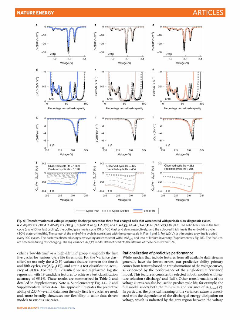
Fig. 4 | transformations of voltage–capacity discharge curves for three fast-charged cells that were tested with periodic slow diagnostic cycles. a–c, dQ/dV at C/10; d–f, dV/dQ at C/10; g–i, dQ/dV at 4 C; j–l, ΔQ(V) at 4 C. a,d,g,j, 4 C/4 C; b,e,h,k, 6 C/4 C; c,f,i,l, 8 C/4 C. The solid black line is the first cycle (cycle 10 for fast cycling), the dotted grey line is cycle 101 or 100 (fast and slow, respectively) and the coloured thick line is the end-of-life cycle (80% state-of-health). The colour of the end-of-life cycle is consistent with the colour scale in Figs. 1 and 2. For ΔQ(V), a thin dotted grey line is added every 100 cycles. The patterns observed using slow cycling are consistent with LAMdeNE and loss of lithium inventory (Supplementary Fig. 18). The features are smeared during fast charging. The log variance ΔQ(V) model dataset predicts the lifetime of these cells within 15%.

NAtuRe eNeRgY | www.nature.com/natureenergy

Articles NATUre eNergy

curves in Fig. 2a. The integral of this region is the total change in energy dissipation between cycles under galvanostatic conditions and is linearly related to the mean of ΔQ(V). Zero variance would indicate energy dissipations that are independent of voltage. Thus, the variance of ΔQ(V) reflects the extent of non-uniformity in the energy dissipation with voltage, due to either open-circuit or kinetic processes, a point that we return to later.

We observe that features derived from early-cycle discharge volt-age curves have excellent predictive performance, even before the onset of capacity fade. We rationalize this observation by investigat-ing degradation modes that do not immediately result in capacity fade yet still manifest in the discharge voltage curve and are also linked to rapid capacity fade near the end of life.

While our data-driven approach has successfully revealed pre-dictive features from early-cycle discharge curves, identification of degradation modes using only high-rate data is challenging because of the convolution of kinetics with open-circuit behaviour. Thus, we turn to established methods for mechanism identification using low-rate cycling data. Dubarry et al.61 mapped degradation modes in LFP/graphite cells to their resultant shift in dQ/dV and dV/dQ derivatives for diagnostic cycles at C/20. One degradation mode—loss of active material of the delithiated negative electrode (LAMdeNE)—results in a shift in discharge voltage with no change in capacity. This behaviour is observed when the negative elec-trode capacity is larger than that of the positive electrode, as is the case in these LFP/graphite cells. Thus, a loss of delithiated nega-tive electrode material changes the potentials at which lithium ions are stored without changing the overall capacity50,61. As proposed by Anséan et al.50, at high rates of LAMdeNE, the negative electrode capacity will eventually fall below the remaining lithium-ion inven-tory. At this point, the negative electrode will not have enough sites to accommodate lithium ions during charging, inducing lithium plating50. Since plating is an additional source of irreversibility, the capacity loss accelerates. Thus, in early cycles, LAMdeNE shifts the voltage curve without affecting the capacity fade curve and induces rapid capacity fade at high cycle number. This degradation mode,

in conjunction with loss of lithium inventory, is widely observed in commercial LFP/graphite cells operated under similar condi-tions32,50–54. We note that the graphitic negative electrode is common to nearly all commercial lithium-ion batteries in use today.

To investigate the contribution of LAMdeNE, we perform addi-tional experiments for cells cycled with varied charging rates (4 C, 6 C and 8 C) and a constant discharge rate (4 C), incorporating slow cycling at the 1st, 100th and end-of-life cycles. Derivatives of diag-nostic discharge curves at C/10 (Fig. 4, rows 1 and 2) are compared with these, and ΔQ(V), at 4 C at the 10th, 101st and end-of-life cycles (rows 3 and 4). The shifts in dQ/dV and dV/dQ observed in diagnostic cycling correspond to a shift of the potentials at which lithium is stored in graphite during charging and are consistent with LAMdeNE and loss of lithium inventory operating concurrently (Supplementary Fig. 18)50,51,61. The magnitude of these shifts from the 1st to 100th cycle increases with charging rate (Supplementary Note 5 and Supplementary Fig. 19). These observations rationalize why models using features based on discharge curves have lower errors than models using only features based on capacity fade curves, since LAMdeNE does not manifest in capacity fade in early cycles. We note that LAMdeNE alters a fraction of, rather than the entire, discharge voltage curve, consistent with the strong correla-tion between the variance of ΔQ(V) and cycle life (Fig. 2c). In sum-mary, we attribute the success of our predictive models to features that capture changes in both the capacity fade curves and voltage curves, since degradation may be silent in discharge capacity but present in voltage curves.

As noted above, differential methods such as dQ/dV and dV/dQ are used extensively to pinpoint degradation mechanisms50,51,53,59–61. These approaches require low-rate diagnostic cycles, as higher rates smear out features due to heterogeneous de(intercalation)32, as seen by comparing row 1 with row 3 in Fig. 4. However, these diagnostic cycles often induce a temporary capacity recovery, commonly observed in cells when the geometric area of the nega-tive electrode exceeds that of the positive electrode56,57. As such, they interrupt the trajectory of capacity fade (Supplementary Fig. 20). Therefore, by applying summary statistics to ΔQ(V) col-lected at high rate, we simultaneously avoid both low-rate diagnostic cycles and numerical differentiation, which decreases the signal-to-noise ratio65. However, these high-rate discharge voltage curves can additionally reflect both kinetic degradation modes and het-erogeneities that are not observed in dQ/dV and dV/dQ curves at C/10. We consider the influence of kinetic degradation modes in Supplementary Note 6, Supplementary Fig. 21 and Supplementary Tables 7–8); briefly, we estimate that low-rate modes such as LAMdeNE primarily contribute (50–80%) to ΔQ(V). We also men-tion that low-rate degradation modes such as LAMdeNE influence the kinetics at high rate, in this case by increasing the local current density of the active regions.

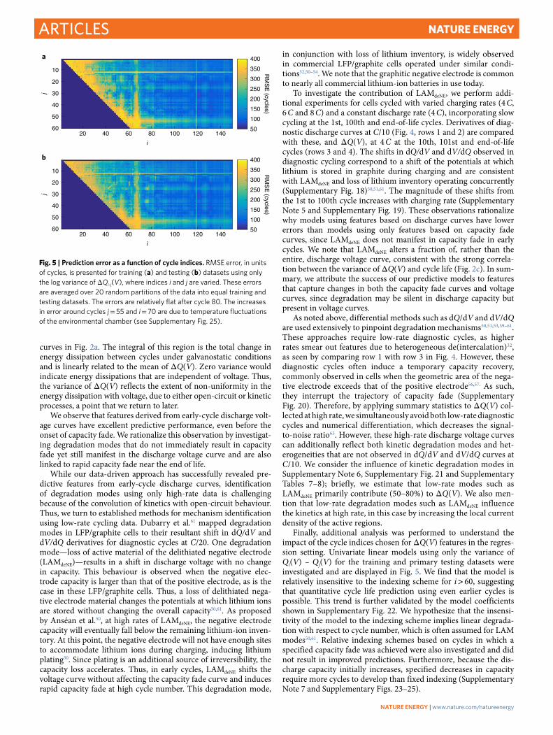
Finally, additional analysis was performed to understand the impact of the cycle indices chosen for ΔQ(V) features in the regres-sion setting. Univariate linear models using only the variance of Qi(V) – Qj(V) for the training and primary testing datasets were investigated and are displayed in Fig. 5. We find that the model is relatively insensitive to the indexing scheme for i > 60, suggesting that quantitative cycle life prediction using even earlier cycles is possible. This trend is further validated by the model coefficients shown in Supplementary Fig. 22. We hypothesize that the insensi-tivity of the model to the indexing scheme implies linear degrada-tion with respect to cycle number, which is often assumed for LAM modes50,61. Relative indexing schemes based on cycles in which a specified capacity fade was achieved were also investigated and did not result in improved predictions. Furthermore, because the dis-charge capacity initially increases, specified decreases in capacity require more cycles to develop than fixed indexing (Supplementary Note 7 and Supplementary Figs. 23–25).

20 40 60 80 100 120 140

i

10

20

30

40

50

60

j

50

100

150

200

250

300

350

400

RM

SE

(cycles)

20 40 60 80 100 120 140

i

10

20

30

40

50

60

j

50

100

150

200

250

300

350

400

RM

SE

(cycles)

a

b

Fig. 5 | Prediction error as a function of cycle indices. RMSE error, in units of cycles, is presented for training (a) and testing (b) datasets using only the log variance of ΔQi-j(V), where indices i and j are varied. These errors are averaged over 20 random partitions of the data into equal training and testing datasets. The errors are relatively flat after cycle 80. The increases in error around cycles j = 55 and i = 70 are due to temperature fluctuations of the environmental chamber (see Supplementary Fig. 25).

NAtuRe eNeRgY | www.nature.com/natureenergy

ArticlesNATUre eNergy

ConclusionsData-driven modelling is a promising route for diagnostics and prognostics of lithium-ion batteries and enables emerging applica-tions in their development, manufacturing and optimization. We develop cycle life prediction models using early-cycle discharge data yet to exhibit capacity degradation, generated from commercial LFP/graphite batteries cycled under fast-charging conditions. In the regression setting, we obtain a test error of 9.1% using only the first 100 cycles; in the classification setting, we obtain a test error of 4.9% using data from the first 5 cycles. This level of accuracy is achieved by extracting features from high-rate discharge voltage curves as opposed to only from the capacity fade curves, and without using data from slow diagnostic cycles or assuming prior knowledge of cell chemistry and degradation mechanisms. The success of the model is rationalized by demonstrating consistency with degrada-tion modes that do not manifest in capacity fade during early cycles but impact the voltage curves. In general, our approach can comple-ment approaches based on physical and semi-empirical models and on specialized diagnostics. Broadly speaking, this work highlights the promise of combining data generation and data-driven mod-elling for understanding and developing complex systems such as lithium-ion batteries.

MethodsCell cycling and data generation. 124 commercial high-power LFP/graphite A123 APR18650M1A cells were used in this work. The cells have a nominal capacity of 1.1 Ah and a nominal voltage of 3.3 V. The manufacturer’s recommended fast-charging protocol is 3.6 C constant current–constant voltage (CC-CV). The rate capability of these cells during charge and discharge is shown in Supplementary Fig. 27.

All cells were tested in cylindrical fixtures with four-point contacts on a 48-channel Arbin LBT battery testing cycler. The tests were performed at a constant temperature of 30 °C in an environmental chamber (Amerex Instruments). Cell can temperatures were recorded by stripping a small section of the plastic insulation and contacting a type T thermocouple to the bare metal casing using thermal epoxy (OMEGATHERM 201) and Kapton tape.

The cells were cycled with various candidate fast-charging policies (Supplementary Table 9) but identically discharged. Cells were charged from 0% to 80% state-of-charge (SOC) with one of 72 different one-step and two-step charging policies. Each step is a single C rate applied over a given SOC range; for example, a two-step policy could consist of a 6 C charging step from 0% to 50% SOC, followed by a 4 C step from 50% to 80% SOC. The 72 charging polices represent different combinations of current steps within the 0% to 80% SOC range. The charging time from 0% to 80% SOC ranged from 9 to 13.3 min. An internal resistance measurement was obtained during charging at 80% SOC by averaging 10 pulses of ±3.6 C with a pulse width of 30 or 33 ms, where 1 C is 1.1 A, or the current required to fully (dis)charge the nominal capacity (1.1 Ah) in 1 h. All cells then charged from 80% to 100% SOC with a uniform 1 C CC-CV charging step to 3.6 V and a current cutoff of C/50. All cells were subsequently discharged with a CC-CV discharge at 4 C to 2.0 V with a current cutoff of C/50. The voltage cutoffs used in this work follow those recommended by the manufacturer.

Our dataset is described in Supplementary Table 9. In total, our dataset consists of three ‘batches’, or cells run in parallel. Each batch has slightly different testing conditions. For the ‘2017-05-12’ batch, the rests after reaching 80% SOC during charging and after discharging were 1 min and 1 s, respectively. For the ‘2017-06-30’ batch, the rests after reaching 80% SOC during charging and after discharging were both 5 min. For the ‘2018-04-12’ batch, 5 s rests were placed after reaching 80% SOC during charging, after the internal resistance test and before and after discharging.

A histogram of cycle life for the three datasets is presented in Supplementary Fig. 28. We note that four cells had unexpectedly high measurement noise and were excluded from analysis.

To standardize the voltage–capacity data across cells and cycles, all 4 C discharge curves were fitted to a spline function and linearly interpolated (Supplementary Fig. 29). Capacity was fitted as a function of voltage and evaluated at 1,000 linearly spaced voltage points from 3.5 V to 2.0 V. These uniformly sized vectors enabled straightforward data manipulations such as subtraction.

Machine-learning model development. This study involved both model fitting (setting the coefficient values) and model selection (setting the model structure). To perform these tasks simultaneously, a regularization technique was employed. A linear model of the form

ŷ = w x (1)i iT

was proposed, where ŷi is the predicted number of cycles for battery i, xi is a p-dimensional feature vector for battery i and w is a p-dimensional model coefficient vector. When applying regularization techniques, a penalty term is added to the least-squares optimization formulation to avoid overfitting. Two regularization techniques, the lasso66 and the elastic net58, simultaneously perform model fitting and selection by finding sparse coefficient vectors. The formulation is

λ = ∥ − ∥ + Pw y Xw wargmin ( ) (2)w 22

where the argmin function represents finding the value of w that minimizes the argument, y is the n-dimensional vector of observed battery lifetimes, X is the n × p matrix of features, and λ is a non-negative scalar. The first term

∥ − ∥y Xw (3)22

is found in ordinary least squares. The formulation of the second term, P(w), depends on the regularization technique being employed. For the lasso,

= ∥ ∥P w w( ) , (4)1

and for the elastic net,

α α= − ∥ ∥ + ∥ ∥P w w w( ) 12

(5)22

1

where α is a scalar between 0 and 1. Both formulations will result in sparse models. The elastic net has been shown to perform better when p » n58, as is often the case in feature engineering applications, but requires fitting an additional hyperparameter (α and λ, as opposed to only λ in the lasso). The elastic net is also preferred when there are high correlations between the features, as is the case in this application. To choose the values of the hyperparameters, we apply four-fold cross-validation and Monte Carlo sampling.

The model development dataset is divided into two equal sections, referred to as the training and primary testing sets. These two sections are chosen such that each spans the range of cycle lives (see Supplementary Table 9). The training data are used to choose the hyper-parameters α and λ and determine the values of the coefficients, w. The training data are further subdivided into calibration and validation sets for cross-validation. The primary test set is then used as a measure of generalizability. The secondary test dataset was generated after model development.

RMSE and average percentage error are chosen to evaluate model performance. RMSE is defined as

∑ ŷ= −=n

yRMSE 1 ( ) (6)i

n

i i1

2

where yi is the observed cycle life, ŷi is the predicted cycle life and n is the total number of samples. The average percentage error is defined as

∑ŷ

=∣ − ∣

×=n

yy

% err 1 100 (7)i

ni i

i1

where all variables are defined as above.To summarize our procedure, we first divide the data into training and test sets.

We then train the model on the training set using the elastic net, yielding a linear model with downselected features and coefficients. Finally, we apply the model to the primary and secondary test sets.

The data processing and elastic net prediction is performed in MATLAB, while the classification is performed in Python using the NumPy, pandas and sklearn packages.

Data availabilityThe datasets used in this study are available at https://data.matr.io/1.

Code availabilityCode for data processing is available at https://github.com/rdbraatz/data-driven-prediction-of-battery-cycle-life-before-capacity-degradation. Code for the modelling work is available from the corresponding authors upon request.

Received: 2 October 2018; Accepted: 18 February 2019; Published: xx xx xxxx

References 1. Dunn, B., Kamath, H. & Tarascon, J.-M. Electrical energy storage for the grid:

a battery of choices. Science 334, 928–935 (2011). 2. Nykvist, B. & Nilsson, M. Rapidly falling costs of battery packs for electric

vehicles. Nat. Clim. Change 5, 329–332 (2015).

NAtuRe eNeRgY | www.nature.com/natureenergy

Articles NATUre eNergy

3. Schmuch, R., Wagner, R., Hörpel, G., Placke, T. & Winter, M. Performance and cost of materials for lithium-based rechargeable automotive batteries. Nat. Energy 3, 267–278 (2018).

4. Peterson, S. B., Apt, J. & Whitacre, J. F. Lithium-ion battery cell degradation resulting from realistic vehicle and vehicle-to-grid utilization. J. Power Sources 195, 2385–2392 (2010).

5. Ramadesigan, V. et al. Modeling and simulation of lithium-ion batteries from a systems engineering perspective. J. Electrochem. Soc. 159, R31–R45 (2012).

6. Waag, W., Fleischer, C. & Sauer, D. U. Critical review of the methods for monitoring of lithium-ion batteries in electric and hybrid vehicles. J. Power Sources 258, 321–339 (2014).

7. Paul, S., Diegelmann, C., Kabza, H. & Tillmetz, W. Analysis of ageing inhomogeneities in lithium-ion battery systems. J. Power Sources 239, 642–650 (2013).

8. Schuster, S. F. et al. Nonlinear aging characteristics of lithium-ion cells under different operational conditions. J. Energy Storage 1, 44–53 (2015).

9. Schuster, S. F., Brand, M. J., Berg, P., Gleissenberger, M. & Jossen, A. Lithium-ion cell-to-cell variation during battery electric vehicle operation. J. Power Sources 297, 242–251 (2015).

10. Harris, S. J., Harris, D. J. & Li, C. Failure statistics for commercial lithium ion batteries: a study of 24 pouch cells. J. Power Sources 342, 589–597 (2017).

11. Baumhöfer, T., Brühl, M., Rothgang, S. & Sauer, D. U. Production caused variation in capacity aging trend and correlation to initial cell performance. J. Power Sources 247, 332–338 (2014).

12. Bloom, I. et al. An accelerated calendar and cycle life study of Li-ion cells. J. Power Sources 101, 238–247 (2001).

13. Broussely, M. et al. Aging mechanism in Li ion cells and calendar life predictions. J. Power Sources 97–98, 13–21 (2001).

14. Christensen, J. & Newman, J. A mathematical model for the lithium-ion negative electrode solid electrolyte interphase. J. Electrochem. Soc. 151, A1977 (2004).

15. Pinson, M. B. & Bazant, M. Z. Theory of SEI formation in rechargeable batteries: capacity fade, accelerated aging and lifetime prediction. J. Electrochem. Soc. 160, A243–A250 (2012).

16. Arora, P. Mathematical modeling of the lithium deposition overcharge reaction in lithium-ion batteries using carbon-based negative electrodes. J. Electrochem. Soc. 146, 3543 (1999).

17. Yang, X.-G., Leng, Y., Zhang, G., Ge, S. & Wang, C.-Y. Modeling of lithium plating induced aging of lithium-ion batteries: transition from linear to nonlinear aging. J. Power Sources 360, 28–40 (2017).

18. Christensen, J. & Newman, J. Cyclable lithium and capacity loss in Li-ion cells. J. Electrochem. Soc. 152, A818–A829 (2005).

19. Zhang, Q. & White, R. E. Capacity fade analysis of a lithium ion cell. J. Power Sources 179, 793–798 (2008).

20. Wright, R. B. et al. Power fade and capacity fade resulting from cycle-life testing of advanced technology development program lithium-ion batteries. J. Power Sources 119–121, 865–869 (2003).

21. Ramadesigan, V. et al. Parameter estimation and capacity fade analysis of lithium-ion batteries using reformulated models. J. Electrochem. Soc. 158, A1048–A1054 (2011).

22. Cordoba-Arenas, A., Onori, S., Guezennec, Y. & Rizzoni, G. Capacity and power fade cycle-life model for plug-in hybrid electric vehicle lithium-ion battery cells containing blended spinel and layered-oxide positive electrodes. J. Power Sources 278, 473–483 (2015).

23. Burns, J. C. et al. Evaluation of effects of additives in wound Li-ion cells through high precision coulometry. J. Electrochem. Soc. 158, A255–A261 (2011).

24. Burns, J. C. et al. Predicting and extending the lifetime of Li-ion batteries. J. Electrochem. Soc. 160, A1451–A1456 (2013).

25. Chen, C. H., Liu, J. & Amine, K. Symmetric cell approach and impedance spectroscopy of high power lithium-ion batteries. J. Power Sources 96, 321–328 (2001).

26. Tröltzsch, U., Kanoun, O. & Tränkler, H.-R. Characterizing aging effects of lithium-ion batteries by impedance spectroscopy. Electrochim. Acta 51, 1664–1672 (2006).

27. Love, C. T., Virji, M. B. V., Rocheleau, R. E. & Swider-Lyons, K. E. State-of-health monitoring of 18650 4S packs with a single-point impedance diagnostic. J. Power Sources 266, 512–519 (2014).

28. Waldmann, T. et al. A mechanical aging mechanism in lithium-ion batteries. J. Electrochem. Soc. 161, A1742–A1747 (2014).

29. Waldmann, T. et al. Influence of cell design on temperatures and temperature gradients in lithium-ion cells: an in operando study. J. Electrochem. Soc. 162, A921–A927 (2015).

30. Bach, T. C. et al. Nonlinear aging of cylindrical lithium-ion cells linked to heterogeneous compression. J. Energy Storage 5, 212–223 (2016).

31. Harris, S. J. & Lu, P. Effects of inhomogeneities—nanoscale to mesoscale—on the durability of Li-ion batteries. J. Phys. Chem. C 117, 6481–6492 (2013).

32. Lewerenz, M., Marongiu, A., Warnecke, A. & Sauer, D. U. Differential voltage analysis as a tool for analyzing inhomogeneous aging: a case study for LiFePO4|graphite cylindrical cells. J. Power Sources 368, 57–67 (2017).

33. Raccuglia, P. et al. Machine-learning-assisted materials discovery using failed experiments. Nature 573, 73–77 (2016).

34. Ward, L., Agrawal, A., Choudhary, A. & Wolverton, C. A general-purpose machine learning framework for predicting properties of inorganic materials. NPJ Comput. Mater. 2, 16028 (2016).

35. Segler, M. H. S., Preuss, M. & Waller, M. P. Planning chemical syntheses with deep neural networks and symbolic AI. Nature 555, 604–610 (2018).

36. Jain, A. et al. Commentary: The Materials Project: a materials genome approach to accelerating materials innovation. APL Mater. 1, 011002 (2013).

37. Aykol, M. et al. High-throughput computational design of cathode coatings for Li-ion batteries. Nat. Commun. 7, 13779 (2016).

38. Sendek, A. D. et al. Holistic computational structure screening of more than 12000 candidates for solid lithium-ion conductor materials. Energy Environ. Sci. 10, 306–320 (2017).

39. Ulissi, Z. W. et al. Machine-learning methods enable exhaustive searches for active bimetallic facets and reveal active site motifs for CO2 reduction. ACS Catal. 7, 6600–6608 (2017).

40. Si, X.-S., Wang, W., Hu, C.-H. & Zhou, D.-H. Remaining useful life estimation—a review on the statistical data driven approaches. Eur. J. Oper. Res. 213, 1–14 (2011).

41. Wu, L., Fu, X. & Guan, Y. Review of the remaining useful life prognostics of vehicle lithium-ion batteries using data-driven methodologies. Appl. Sci. 6, 166 (2016).

42. Saha, B., Goebel, K. & Christophersen, J. Comparison of prognostic algorithms for estimating remaining useful life of batteries. Trans. Inst. Meas. Control 31, 293–308 (2009).

43. Nuhic, A., Terzimehic, T., Soczka-Guth, T., Buchholz, M. & Dietmayer, K. Health diagnosis and remaining useful life prognostics of lithium-ion batteries using data-driven methods. J. Power Sources 239, 680–688 (2013).

44. Hu, C., Jain, G., Tamirisa, P. & Gorka, T. Method for estimating the capacity and predicting remaining useful life of lithium-ion battery. Appl. Energy 126, 182–189 (2014).

45. Miao, Q., Xie, L., Cui, H., Liang, W. & Pecht, M. Remaining useful life prediction of lithium-ion battery with unscented particle filter technique. Microelectron. Reliab. 53, 805–810 (2013).

46. Hu, X., . & Jiang, J. & Cao, D. & Egardt, B. Battery health prognosis for electric vehicles using sample entropy and sparse Bayesian predictive modeling. IEEE Trans. Ind. Electron. 63, 2645–2656 (2016).

47. Zhang, Y., . & Xiong, R. & He, H. & Pecht, M. Lithium-ion battery remaining useful life prediction with Box–Cox transformation and Monte Carlo simulation. IEEE Trans. Ind. Electron. 66, 1585–1597 (2019).

48. Zhang, Y., & Xiong, R. & He, H. & Pecht, M. Long short-term memory recurrent neural network for remaining useful life prediction of lithium-ion batteries. IEEE Trans. Veh. Technol. 67, 5695–5705 (2018).

49. Saha, B. & Goebel, K. Battery data set. NASA Ames Progn. Data Repos. (2007). 50. Anseán, D. et al. Fast charging technique for high power LiFePO4

batteries: a mechanistic analysis of aging. J. Power Sources 321, 201–209 (2016).

51. Anseán, D. et al. Operando lithium plating quantification and early detection of a commercial LiFePO4 cell cycles under dynamic driving schedule. J. Power Sources 356, 36–46 (2017).

52. Liu, P. et al. Aging mechanisms of LiFePO4 batteries deduced by electrochemical and structural analyses. J. Electrochem. Soc. 157, A499–A507 (2010).

53. Safari, M. & Delacourt, C. Aging of a commercial graphite/LiFePO4 cell. J. Electrochem. Soc. 158, A1123–A1135 (2011).

54. Sarasketa-Zabala, E. et al. Understanding lithium inventory loss and sudden performance fade in cylindrical cells during cycling with deep-discharge steps. J. Phys. Chem. C 119, 896–906 (2015).

55. Ahmed, S. et al. Enabling fast charging—a battery technology gap assessment. J. Power Sources 367, 250–262 (2017).

56. Gyenes, B., Stevens, D. A., Chevrier, V. L. & Dahn, J. R. Understanding anomalous behavior in Coulombic efficiency measurements on Li-ion batteries. J. Electrochem. Soc. 162, A278–A283 (2015).

57. Lewerenz, M. et al. Systematic aging of commercial LiFePO4|graphite cylindrical cells including a theory explaining rise of capacity during aging. J. Power Sources 345, 254–263 (2017).

58. Zou, H. & Hastie, T. Regularization and variable selection via the elastic net. J. R. Stat. Soc. B 67, 301–320 (2005).

59. Bloom, I. et al. Differential voltage analyses of high-power, lithium-ion cells: 1. Technique and application. J. Power Sources 139, 295–303 (2005).

60. Smith, A. J., Burns, J. C. & Dahn, J. R. High-precision differential capacity analysis of LiMn2O4/graphite cells. Electrochem. Solid-State Lett. 14, A39–A41 (2011).

61. Dubarry, M., Truchot, C. & Liaw, B. Y. Synthesize battery degradation modes via a diagnostic and prognostic model. J. Power Sources 219, 204–216 (2012).

62. Berecibar, M. et al. Online state of health estimation on NMC cells based on predictive analytics. J. Power Sources 320, 239–250 (2016).

NAtuRe eNeRgY | www.nature.com/natureenergy

ArticlesNATUre eNergy

63. Berecibar, M., Garmendia, M., Gandiaga, I., Crego, J. & Villarreal, I. State of health estimation algorithm of LiFePO4 battery packs based on differential voltage curves for battery management system application. Energy 103, 784–796 (2016).

64. Birkl, C. R., Roberts, M. R., McTurk, E., Bruce, P. G. & Howey, D. A. Degradation diagnostics for lithium ion cells. J. Power Sources 341, 373–386 (2017).

65. Richardson, R. R., Birkl, C. R., Osborne, M. A. & Howey, D. A. Gaussian process regression for in-situ capacity estimation of lithium-ion batteries. IEEE Trans. Ind. Inform. 15, 127–138 (2019).

66. Tibshirani, R. Regression shrinkage and selection via the lasso. J. R. Stat. Soc. B 58, 267–288 (1996).

AcknowledgementsThis work was supported by Toyota Research Institute through the Accelerated Materials Design and Discovery programme. P.M.A. was supported by the Thomas V. Jones Stanford Graduate Fellowship and the National Science Foundation Graduate Research Fellowship under Grant No. DGE-114747. N.P. was supported by SAIC Innovation Center through Stanford Energy 3.0 industry affiliates programme. S.J.H. was supported by the Assistant Secretary for Energy Efficiency, Vehicle Technologies Office of the US Department of Energy under the Advanced Battery Materials Research Program. We thank E. Reed, S. Ermon, Y. Li, C. Bauemer, A. Grover, T. Markov, D. Deng, A. Baclig and H. Thaman for discussions.

Author contributionsP.M.A., N.J., N.P., M.H.C. and W.C.C. conceived of and conducted the experiments. K.A.S., Z.Y. and B.J. performed the modelling. M.A., Z.Y. and P.K.H. performed data management. P.M.A., K.A.S., N.J., B.J., D.F., M.Z.B., S.J.H., W.C.C. and R.D.B. interpreted the results. All authors edited and reviewed the manuscript. W.C.C. and R.D.B. supervised the work.

Competing interestsK.A.S., R.D.B., W.C.C., P.M.A., N.J., S.J.H. and N.P. have filed a patent related to this work: US Application No. 62/575,565, dated 16 October 2018.

Additional informationSupplementary information is available for this paper at https://doi.org/10.1038/s41560-019-0356-8.

Reprints and permissions information is available at www.nature.com/reprints.

Correspondence and requests for materials should be addressed to W.C.C. or R.D.B.

Publisher’s note: Springer Nature remains neutral with regard to jurisdictional claims in published maps and institutional affiliations.

© The Author(s), under exclusive licence to Springer Nature Limited 2019

NAtuRe eNeRgY | www.nature.com/natureenergy