Data-Driven Learning Models with Applications to Retail ...

Data-Driven Learning Models with Applications toRetail Operations

by

Sajad Modaresi

Business AdministrationDuke University

Date:Approved:

Fernando Bernstein, Supervisor

Nuri Bora Keskin

Robert Swinney

Peng Sun

Dissertation submitted in partial fulfillment of the requirements for the degree ofDoctor of Philosophy in Business Administration

in the Graduate School of Duke University2018

Abstract

Data-Driven Learning Models with Applications to Retail

Operations

by

Sajad Modaresi

Business AdministrationDuke University

Date:Approved:

Fernando Bernstein, Supervisor

Nuri Bora Keskin

Robert Swinney

Peng Sun

An abstract of a dissertation submitted in partial fulfillment of the requirements forthe degree of Doctor of Philosophy in Business Administration

in the Graduate School of Duke University2018

Copyright c© 2018 by Sajad ModaresiAll rights reserved except the rights granted by the

Creative Commons Attribution-Noncommercial Licence

http://creativecommons.org/licenses/by-nc/3.0/us/

Abstract

Data-driven approaches to decision-making under uncertainty is at the center of

many operational problems. These are problems in which there is an element of

uncertainty that needs to be estimated (learned) from data in order to make online

(dynamic) operational decisions. An example of such problems is estimating cus-

tomer demand from transaction data to make dynamic assortment decisions. This

dissertation adopts a data-driven active learning approach to study various opera-

tional problems under uncertainty with a focus on retail operations.

The first two essays in this dissertation study the classic exploration (i.e., pa-

rameter estimation) versus exploitation (i.e., optimization) trade-off from different

perspectives. The first essay takes a theoretical approach and studies such trade-

off in a combinatorial optimization setting. We show that resolving the exploration

versus exploitation trade-off efficiently is related to solving a Lower Bound Problem

(LBP), which simultaneously answers the questions of what to explore and how to do

so. We establish a fundamental limit on the asymptotic performance of any admis-

sible policy that is proportional to the optimal objective value of the LBP problem.

We also propose near-optimal policies that are implementable in real-time. We test

the performance of the proposed policies through extensive numerical experiments

and show that they significantly outperform the relevant benchmark.

The second essay considers the dynamic assortment personalization problem of

an online retailer facing heterogeneous customers with unknown product preferences.

iv

We propose a prescriptive approach, called the dynamic clustering policy, for dynamic

estimation of customer preferences and optimization of personalized assortments. We

test the proposed approach with a case study based on a dataset from a large Chilean

retailer. The case study suggests that the benefits of the dynamic clustering policy

under the Multinomial Logit (MNL) model can be substantial and result (on aver-

age) in more than 37% additional transactions compared to a data-intensive policy

that treats customers independently and in more than 27% additional transactions

compared to a linear-utility policy that assumes that product mean utilities are lin-

ear functions of available customer attributes. We support the insights derived from

the numerical experiments by analytically characterizing settings in which pooling

transaction information is beneficial for the retailer, in a simplified version of the

problem. We also show that there are diminishing marginal returns to pooling in-

formation from an increasing number of customers.

Further focusing on retail operations, the final essay studies the interplay between

a retailer’s return and pricing policies and customers’ purchasing decisions. We char-

acterize the retailer’s optimal prices in the cases with and without product returns

and determine conditions under which offering the return option to customers in-

creases the retailer’s revenue. We also explore the impact of accounting for product

returns on demand estimation. The preliminary numerical results based on a real

dataset suggest that our model, which accounts for product returns, increases de-

mand estimation accuracy compared to models that do not consider product returns

in their estimation.

v

To Grandpa.

vi

Contents

Abstract iv

List of Tables xi

List of Figures xii

List of Abbreviations and Symbols xiv

Acknowledgements xx

1 Introduction 1

2 Learning in Combinatorial Optimization: What and How to Ex-plore 5

2.1 Introduction . . . . . . . . . . . . . . . . . . . . . . . . . . . . . . . . 5

2.2 Literature Review . . . . . . . . . . . . . . . . . . . . . . . . . . . . . 10

2.3 Combinatorial Formulation versus Traditional Bandits . . . . . . . . 13

2.3.1 Problem Formulation . . . . . . . . . . . . . . . . . . . . . . . 13

2.3.2 Known Results and Incorporating Combinatorial Aspects . . . 15

2.4 Bounds on Achievable Asymptotic Performance . . . . . . . . . . . . 19

2.5 An Efficient Practical Policy . . . . . . . . . . . . . . . . . . . . . . . 24

2.6 Computational Aspects for Solving OCP and Policy Implementation . 29

2.6.1 MIP Formulations of OCP for Polynomially-Solvable Problems 30

2.7 Numerical Experiments . . . . . . . . . . . . . . . . . . . . . . . . . . 35

2.7.1 Long-Term Experiments . . . . . . . . . . . . . . . . . . . . . 35

vii

2.7.2 Experiment with Size of the Ground Set . . . . . . . . . . . . 40

2.7.3 Short-Term Experiments . . . . . . . . . . . . . . . . . . . . . 43

2.8 Conclusion . . . . . . . . . . . . . . . . . . . . . . . . . . . . . . . . . 46

3 A Dynamic Clustering Approach to Data-Driven Assortment Per-sonalization 49

3.1 Introduction . . . . . . . . . . . . . . . . . . . . . . . . . . . . . . . . 49


3.3 Model and Preliminaries . . . . . . . . . . . . . . . . . . . . . . . . . 57

3.4 Dynamic Assortment Personalization . . . . . . . . . . . . . . . . . . 63

3.4.1 Bayesian Model of Preferences . . . . . . . . . . . . . . . . . . 63

3.4.2 Dynamic Clustering Policy . . . . . . . . . . . . . . . . . . . . 65

3.4.3 Mapping and Preference Estimation . . . . . . . . . . . . . . . 66

3.4.4 Assortment Optimization . . . . . . . . . . . . . . . . . . . . . 69

3.5 Case Study . . . . . . . . . . . . . . . . . . . . . . . . . . . . . . . . 72

3.5.1 Dataset . . . . . . . . . . . . . . . . . . . . . . . . . . . . . . 72

3.5.2 Implementation Details . . . . . . . . . . . . . . . . . . . . . . 73

3.5.3 Performance Comparison . . . . . . . . . . . . . . . . . . . . . 77

3.5.4 Customer Attributes . . . . . . . . . . . . . . . . . . . . . . . 79

3.5.5 Comparison to Linear-Utility Model . . . . . . . . . . . . . . . 83

3.6 Value of Pooling Information . . . . . . . . . . . . . . . . . . . . . . . 88

3.6.1 Semi-Oracle . . . . . . . . . . . . . . . . . . . . . . . . . . . . 90

3.6.2 Pooling in the Short-Term . . . . . . . . . . . . . . . . . . . . 92

3.7 Conclusion . . . . . . . . . . . . . . . . . . . . . . . . . . . . . . . . . 96

4 Uncertainty in Choice: The Role of Return Policies 98

4.1 Introduction . . . . . . . . . . . . . . . . . . . . . . . . . . . . . . . . 98


viii

4.3 Customer’s Choice Model . . . . . . . . . . . . . . . . . . . . . . . . 102

4.3.1 Non-Returnable Products . . . . . . . . . . . . . . . . . . . . 103

4.3.2 Returnable Products . . . . . . . . . . . . . . . . . . . . . . . 104

4.4 Seller’s Revenue Maximization Problem . . . . . . . . . . . . . . . . . 107

4.5 Analysis and Results . . . . . . . . . . . . . . . . . . . . . . . . . . . 108

4.5.1 Price Optimization for Single-Product Case . . . . . . . . . . 108

4.5.2 Single Price Optimization for Multi-Product Case . . . . . . . 112

4.6 Impact of Product Returns on Demand Estimation . . . . . . . . . . 112

4.7 Conclusion and Future Research . . . . . . . . . . . . . . . . . . . . . 117

5 Conclusion 119

A Appendices for Chapter 2 121

A.1 Omitted Proofs and Materials from Section 2.4 . . . . . . . . . . . . . 121

A.1.1 A Limit on Achievable Performance . . . . . . . . . . . . . . . 121

A.1.2 Family of Instances with Finite Regret . . . . . . . . . . . . . 127

A.1.3 LBP-based policy . . . . . . . . . . . . . . . . . . . . . . . . . 128

A.1.4 Performance Guarantee of the LBP-based policy . . . . . . . . 132

A.1.5 Performance Gap Analysis . . . . . . . . . . . . . . . . . . . . 141

A.1.6 Adjoint Formulation for Tighter Upper Bound . . . . . . . . . 143


A.2.1 Equivalence of LBP and OCP . . . . . . . . . . . . . . . . . . 144

A.2.2 Modified OCP-Based Policy . . . . . . . . . . . . . . . . . . . 146


A.3.1 General Complexity of OCP . . . . . . . . . . . . . . . . . . . 151

A.3.2 Critical Sets for Matroids . . . . . . . . . . . . . . . . . . . . 152

A.3.3 Basic MIP Formulation for OCP . . . . . . . . . . . . . . . . 153

ix

A.3.4 IP Formulation for OCP when Combpνq Admits a CompactIP Formulation . . . . . . . . . . . . . . . . . . . . . . . . . . 154

A.3.5 Linear-sized Formulation of OCP for Shortest Path Problem . 155

A.3.6 A Time-Constrained Asynchronous Policy . . . . . . . . . . . 156

A.3.7 Greedy Oracle Polynomial-Time Heuristic . . . . . . . . . . . 157

A.4 Additional Computational Results . . . . . . . . . . . . . . . . . . . . 158

A.5 Alternative Feedback Setting . . . . . . . . . . . . . . . . . . . . . . . 161

A.6 Auxiliary Result for the Proof of Theorem 6 and Theorem 10 . . . . . 162

B Appendices for Chapter 3 164

B.1 Proofs . . . . . . . . . . . . . . . . . . . . . . . . . . . . . . . . . . . 164

B.2 Additional Proofs and Numerical Results . . . . . . . . . . . . . . . . 176

C Appendices for Chapter 4 179

C.1 Proofs . . . . . . . . . . . . . . . . . . . . . . . . . . . . . . . . . . . 179

Bibliography 185

Biography 193

x

List of Tables

2.1 Average total computation time (in seconds) for each replication ofN 20000. . . . . . . . . . . . . . . . . . . . . . . . . . . . . . . . . 42

3.1 Average computation time (in seconds) of different policies for MNLdemand and T 5000. . . . . . . . . . . . . . . . . . . . . . . . . . . 82

3.2 Average computation time (in seconds) of the original and a location-based version of the dynamic clustering policy for MNL demand withI 450 and T 5000. . . . . . . . . . . . . . . . . . . . . . . . . . . 82

3.3 Average percentage improvement of dynamic clustering policy overdata-intensive and linear-utility policies in separation-based experi-ments using the original dataset. . . . . . . . . . . . . . . . . . . . . . 87

3.4 Average estimation time (in seconds) in separation-based experimentsbased on original dataset. . . . . . . . . . . . . . . . . . . . . . . . . 87

4.1 Hard RMSE of different models on a dataset with 30% returns rate. . 116

A.1 Average number of arc trials up to period N 2000, and averagesolution size for different policies on Examples 1, 2 and 28. . . . . . . 160

B.1 Average percentage improvement of dynamic clustering policy overdata-intensive and linear-utility policies in separation-based experi-ments using a synthetic linear dataset. . . . . . . . . . . . . . . . . . 178

xi

List of Figures

2.1 Graph for Example 1 (left), and Example 2 (right). . . . . . . . . . . 17

2.2 Average performance of different policies on the representative settingfor the shortest path (left) and knapsack (right) problems. . . . . . . 39

2.3 Average performance of different policies on the representative settingfor the Steiner tree problem with zero (left) and positive (right) lowerbounds. . . . . . . . . . . . . . . . . . . . . . . . . . . . . . . . . . . 39

2.4 Constants KLS (left) and KFinal (right) when increasing the size ofthe ground set. . . . . . . . . . . . . . . . . . . . . . . . . . . . . . . 42

2.5 Average performance (left) and computation time (right) as a functionof N for the instance with L 10, |A| 41, and |S| 1025. . . . . . 42

2.6 Average performance of different policies on the representative settingfor the shortest path (left), Steiner tree (center) and knapsack (right)problems – the vertical lines show the 95% confidence intervals. . . . 46

3.1 Illustration of the dynamic clustering policy. . . . . . . . . . . . . . . 66

3.2 Example of an assortment shown on the retailer’s website. . . . . . . 74

3.3 Average performance in a market with I 42 profiles and independentdemand (left), and MNL demand (right). . . . . . . . . . . . . . . . . 77

3.4 Speed of learning for different policies (left) and the evolution of theaverage number of clusters under the dynamic clustering policy (right)for MNL demand and I 42. . . . . . . . . . . . . . . . . . . . . . . 79

3.5 Average performance in a market with MNL demand and I 75(left), I 140 (middle), and I 450 (right). . . . . . . . . . . . . . . 80

3.6 Illustration of clusters (under the most likely mapping) for womenfrom age groups r0, 29s (left), r30, 39s (middle), and r40, 99s (right)based on customers’ location in Chile. . . . . . . . . . . . . . . . . . . 85

xii

3.7 Illustration of optimal assortments for women from age group r30, 39s. 85

3.8 Gap between the regrets of data-intensive and dynamic clustering poli-cies as a function of number of profiles. . . . . . . . . . . . . . . . . . 92

4.1 Revenue function for different hassle costs in the case with a singlereturnable product. . . . . . . . . . . . . . . . . . . . . . . . . . . . . 110

4.2 An example of non-unimodality of the revenue function in the casewith two returnable products. . . . . . . . . . . . . . . . . . . . . . . 113

A.1 Graph for Example 28. . . . . . . . . . . . . . . . . . . . . . . . . . . 129

A.2 Average performance of different policies on Examples 1 (left), 2 (cen-ter) and 28 (right). . . . . . . . . . . . . . . . . . . . . . . . . . . . . 159

A.3 Box plots of performance for OCP-based and benchmark policies onExamples 1 (left), 2 (center) and 28 (right). . . . . . . . . . . . . . . 160

xiii

List of Abbreviations and Symbols

Symbols

Notation for Chapter 2

The notation xpaq refers to the a-th element of vector x.

A Ground set.

S;S Set of all feasible solutions of the underlying combinatorial prob-lem; A feasible solution.

N Total number of periods.

Bn Random cost coefficient vector in period n.

F Common distribution of the cost coefficient vector.

l Vector of lower bounds on the range of F .

u Vector of upper bounds on the range of F .

Sn Solution implemented in period n.

bn Realized cost coefficient vector in period n.

π A non-anticipating policy.

Fn Filtration (history) in period n.

E Expectation.

Jπpq;Rπpq Expected cumulative cost associated with policy π; Regret asso-ciated with policy π.

Combpνq Underlying combinatorial optimization problem given the costvector ν.

xiv

zCombpνq Optimal objective value of the underlying combinatorial problemgiven the cost vector ν.

Spνq Set of optimal solutions to the underlying combinatorial problemgiven the cost vector ν.

µ Mean cost coefficient vector.

1 tu Indicator function of a set.

Tnpaq Number of trials of ground element a prior to period n.

∆νS Optimality gap associated with solution S given the cost vector

ν.

LBP Lower Bound Problem.

zLBP Optimal objective value of the LBP problem.

π LBP-based policy.

OCP pνq Optimality Cover Problem given the cost vector ν.

zOCP pνq Optimal objective value of the OCP problem given the cost vec-tor ν.

ΓOCP pνq Set of optimal solutions to the OCP problem given the cost vec-tor ν.

pµn Vector of sample means of cost realizations of ground elementsprior to period n.

ni Starting period of cycle i.

H Tuning parameter of the OCP-based policy.

πOCP OCP-based policy.

convpq Convex hull of a set.

diagpνq Diagonal matrix with vector ν as its diagonal.


Superscript i refers to profile i and subscripts j and t refer to product j and time

(customer arrival) t, respectively. Moreover, the notation y denotes an estimate for

a parameter y and y denotes a threshold on the value of a parameter y.

xv

T Total number of customer arrivals.

N ;N Total number of products; Set of all products.

I; I Total number of profiles; Set of all profiles.

Ik; Ik Number of profiles in cluster k; Set of profiles in cluster k.

C Display constraint.

rj Price of product j.

xi Unique vector of attributes associated with profile i.

pi Arrival probability of profile i.

Pk Proportion of profiles in cluster k.

it Profile of customer t.

St;Si Assortment offered to customer t; Optimal assortment for profile

i.

Zij,t Purchasing decision of a customer with profile i arriving at time

t regarding product j.

U ij,t Random utility of product j for a customer with profile i arriving

at time t.

µij;µi Preference parameter of product j for profile i; Vector of prefer-

ence parameters for profile i.

ζ ij,t Standard Gumbel random variables.

νij Exponentiated mean utility of product j for profile i.

ΠjpS, µiq Purchase probability of product j for profile i given an assort-

ment S.

Ft Filtration (history) at time t.

π An admissible assortment selection policy.

P ;P 1 Set of all admissible policies; Set of all admissible consistentpolicies.

Eπ Expectation when policy π is used.

Jπpq;Rπpq Expected cumulative revenue of policy π; Regret associated withpolicy π.

xvi

M Mapping of profiles to clusters.

K;K Total number of clusters; Set of all clusters.

F pq Probability distribution of purchasing decisions.

DP pH0, αq Dirichlet Process with baseline prior distribution H0 and preci-sion parameter α.

X it Assortment and purchase history associated with profile i at time

t.

η Number of MCMC iterations.

ci; ci Cluster associated with profile i; Candidate cluster for profile i.

ni,c Number of profiles, excluding profile i, that are mapped to clus-ter c.

Lpq Likelihood function.

apci , ciq Acceptance probability of changing ci to ci .

fi Frequency proportion associated with mapping Mi.

Betapaj,t, bj,tq Beta distribution with parameters aj,t and bj,t.

Qj,t Index of product j at time t.

µj Sample mean of the number of purchases for product j.

kjpt 1q Number of times that product j has been offered up to time t1.

Qj,t Index of product j at time t.

Rdc Regret of dynamic clustering policy.

Rd-int Regret of data-intensive policy.

Rs-orc Regret of semi-oracle policy.

Rpool Regret of pooling policy.

Us-orc;Upool Upper bound on the regret of semi-oracle policy; Upper boundon the regret of pooling policy.

Ld-int Lower bound on the regret of data-intensive policy.

G1;G2 Gap function between the regret of data-intensive and semi-oracle policies; Gap function between the regret of data-intensiveand pooling policies.

xvii

G1l;G2l Approximate lower bound for the gap function G1; Approximatelower bound for the gap function G2.


The notation y denotes a threshold on the value of a parameter y.

n Total number of products.

S A subset (assortment) of products.

UNRi Random utility obtained from purchasing product i in the case

with no-returns.

βi Nominal mean utility of product i.

pi; p Price of product i; Vector of all product prices.

wi Nominal mean utility of product i minus its price.

µ1 Degree of heterogeneity between products.

εi Customer’s pre-purchase uncertainty.

PNRi Purchase probability of product i in the case with no-returns.

Ukeepi Random utility obtained from keeping product i.

U returni Random utility obtained from returning product i.

c Customer’s hassle cost of return.

µ2 Degree of heterogeneity between keeping and returning options.

εkeepi Customer’s post-purchase uncertainty for keeping product i.

εreturni Customer’s post-purchase uncertainty for returning product i.

Preturni Return probability of product i.

URi Random utility obtained from purchasing product i in the case

with returns.

Ai Expected utility of purchasing product i.

PRi Purchase probability of product i in the case with returns.

k Mean utility of the outside option in the case with returns.

xviii

π0; π1 Seller’s expected revenue in the case with no-returns; Seller’sexpected revenue in the case with returns.

π0 ; π1 Seller’s optimal expected revenue in the case with no-returns;Seller’s optimal expected revenue in the case with returns.

p0 ; p1 Optimal price in the case with no-returns; Optimal price in thecase with returns.

Abbreviations

IID Independent and Identically Distributed.

MIP Mixed Integer Programming.

MNL Multinomial Logit.

N-MNL Nested Multinomial Logit.

MCMC Markov Chain Monte Carlo.

MLE Maximum Likelihood Estimation.

RMSE Root Mean Squared Error.

xix

Acknowledgements

I would like to express my deepest gratitude to my current and former advisors,

Professors Fernando Bernstein, Denis Saure, and Juan Pablo Vielma, for all their

guidance, support, and encouragement throughout my Ph.D. studies. I would also

like to thank the members of my dissertation committee, Professors Bora Keskin,

Peng Sun, and Robert Swinney. Their suggestions have significantly improved this

dissertation.

I am thankful to other faculty members at Duke, particularly, Professors Jean-

nette Song, Kevin Shang, Pranab Majumder, David Brown, and Jim Smith. I am

also grateful to my dear friends, Professors Arian Aflaki, Safak Yucel, and Asa Pal-

ley, who graduated from Duke. I am also thankful to my Ph.D. fellow friends at

Fuqua, Soudipta Chakraborty, Chengyu Wu, Andrew Frazelle, Vinh Nguyen, Yunke

Mai, Huseyin Gurkan, Levi DeValve, Zhenhuan Lei, Yuan-Mao Kao, Shuyu Chen,

Yuan Guo, Yuexing Li, and Chen-An Lin.

Finally, I would like to thank my parents, Yousef and Maliheh, my twin brother,

Sina, my sister, Zahra, and my grandparents, for all their unconditional love, whole-

hearted support, and great encouragement. Last but not least, I would like to thank

my girlfriend, Forough, for her deep love, loving kindness, and tremendous support.

xx

1

Introduction

Data-driven approaches to decision-making under uncertainty is at the center of

many operational problems. These are problems in which there is an element of un-

certainty that needs to be estimated (learned) from data in order to make dynamic

operational decisions. For instance, consider shortest path problems in network ap-

plications where the arc costs (travel times) are stochastic due to network traffic

(congestion). Another example in the context of retail operations is the dynamic

assortment planning problem of a retailer facing customers with unknown demand.

When possible, the uncertain model parameters are estimated offline by using his-

torical data. However, offline estimation is not always possible as, for example,

historical data (if available) might only provide partial information about uncertain

model parameters. For example, a retailer offering a new assortment of products at

the beginning of a new selling season has no (or limited) prior information about

customer demand for such products. In such settings, the parameter estimation

(e.g., demand estimation) must be conducted online by actively collecting data (e.g.,

customer transaction data), and dynamically revisited as more information becomes

available. In doing so, one must balance the classic exploration (i.e., parameter

1

estimation) versus exploitation (i.e., optimization) trade-off.

This dissertation adopts a data-driven active learning approach to study various

operational problems under uncertainty with a focus on retail operations. The first

two essays in this dissertation study the exploration versus exploitation trade-off

from different perspectives. The first essay takes a theoretical approach and stud-

ies such trade-off in a combinatorial optimization setting. Our paper is the first to

prove a lower bound on the asymptotic performance of any admissible policy. We

also propose near-optimal policies that are implementable in real-time. The second

essay studies the dynamic assortment personalization problem of an online retailer

facing heterogeneous customers with unknown product preferences. We propose a

prescriptive approach, called the dynamic clustering policy, for dynamic estimation

of customer preferences and optimization of personalized assortments. Further fo-

cusing on retail operations, the final essay studies the interplay between a retailer’s

return and pricing policies and customers’ purchasing decisions. We characterize the

retailer’s optimal prices in the cases with and without product returns and deter-

mine conditions under which offering the return option to customers increases the

retailer’s revenue. We also explore the impact of accounting for product returns on

demand estimation.

In the first essay, Learning in Combinatorial Optimization: What and How to

Explore (joint work with Denis Saure and Juan Pablo Vielma), we study dynamic

decision-making under uncertainty when, at each period, a decision-maker imple-

ments a solution to a combinatorial optimization problem. The objective coefficient

vectors of said problem, which are unobserved prior to implementation, vary from

period to period. These vectors, however, are known to be random draws from an

initially unknown distribution with known range. By implementing different solu-

tions, the decision-maker extracts information about the underlying distribution, but

at the same time experiences the cost associated with said solutions. We show that

2

resolving the implied exploration versus exploitation trade-off efficiently is related

to solving a Lower Bound Problem (LBP), which simultaneously answers the ques-

tions of what to explore and how to do so. We establish a fundamental limit on the

asymptotic performance of any admissible policy that is proportional to the optimal

objective value of the LBP problem. We show that such a lower bound might be

asymptotically attained by policies that adaptively reconstruct and solve LBP at an

exponentially decreasing frequency. Because LBP is likely intractable in practice,

we propose policies that instead reconstruct and solve a proxy for LBP. We pro-

vide strong evidence of the practical tractability of said proxy which implies that

the proposed policies can be implemented in real-time. We test the performance of

the proposed policies through extensive numerical experiments and show that they

significantly outperform relevant benchmark in the long-term and are competitive in

the short-term.

In the second essay, A Dynamic Clustering Approach to Data-Driven Assortment

Personalization (joint work with Fernando Bernstein and Denis Saure), we consider

an online retailer facing heterogeneous customers with initially unknown product

preferences. Customers are characterized by a diverse set of demographic and trans-

actional attributes. The retailer can personalize the customers’ assortment offerings

based on available profile information to maximize cumulative revenue. To that end,

the retailer must estimate customer preferences by observing transaction data. This,

however, may require a considerable amount of data and time given the broad range

of customer profiles and large number of products available. At the same time, the

retailer can aggregate (pool) purchasing information among customers with simi-

lar product preferences to expedite the learning process. We propose a dynamic

clustering policy that estimates customer preferences by adaptively adjusting cus-

tomer segments (clusters of customers with similar preferences) as more transaction

information becomes available. We test the proposed approach with a case study

3

based on a dataset from a large Chilean retailer. The case study suggests that the

benefits of the dynamic clustering policy under the MNL model can be substantial

and result (on average) in more than 37% additional transactions compared to a

data-intensive policy that treats customers independently and in more than 27%

additional transactions compared to a linear-utility policy that assumes that prod-

uct mean utilities are linear functions of available customer attributes. We support

the insights derived from the numerical experiments by analytically characterizing

settings in which pooling transaction information is beneficial for the retailer, in a

simplified version of the problem. We also show that there are diminishing marginal

returns to pooling information from an increasing number of customers.

In the final essay, Uncertainty in Choice: The Role of Return Policies (joint work

with Fernando Bernstein and Gustavo Vulcano), we study the interplay between a

retailer’s return and pricing policies and customers’ purchasing decisions. We model

the customers’ purchasing and returns decisions using a discrete choice model and

study the seller’s revenue maximization problem in the cases with and without prod-

uct returns. For the single-product case, we characterize the seller’s optimal price

and show that the return option results in different (but not necessarily higher) opti-

mal prices compared to the case with no returns. Moreover, we find that offering the

return option is not always favorable for the retailer. In addition, we characterize

conditions under which offering the return option to customers increases the retailer’s

revenue. Finally, we numerically study the impact of accounting for product returns

on demand estimation. The preliminary numerical results based on a real dataset

suggest that our model, which accounts for product returns, increases demand esti-

mation accuracy compared to models that do not consider product returns in their

estimation.

4

2

Learning in Combinatorial Optimization: Whatand How to Explore

2.1 Introduction

Motivation. Traditional solution approaches to many operational problems are

based on combinatorial optimization problems and typically involve instantiating

a deterministic mathematical program, whose solution is implemented repeatedly

through time: nevertheless, in practice, instances are not usually known in advance.

When possible, parameters characterizing said instances are estimated off-line, ei-

ther by using historical data or from direct observation of the (idle) system. Unfor-

tunately, off-line estimation is not always possible as, for example, historical data (if

available) might only provide partial information pertaining previously implemented

solutions. Consider, for instance, shortest path problems in network applications:

repeated implementation of a given path might reveal cost information about arcs

on such a path, but might provide no further information about costs of other arcs in

the graph. Similar settings arise, for example, in other network applications (e.g., to-

mography and connectivity) in which feedback about cost follows from instantiating

5

and solving combinatorial problems such as spanning and Steiner trees.

Alternatively, parameter estimation might be conducted on-line using feedback

associated with implemented solutions, and revisited as more information about the

system’s primitives becomes available. In doing so, one must consider the interplay

between the performance of a solution and the feedback generated from its implemen-

tation: some parameters might only be reconstructed by implementing solutions that

perform poorly (relative to the optimal solution). This is an instance of the explo-

ration versus exploitation trade-off which is at the center of many dynamic decision-

making problems under uncertainty, and as such, it can be approached through the

multi-armed bandit paradigm (Robbins, 1952). However, the combinatorial setting

has salient features that distinguish it from the traditional bandit. In particular, the

combinatorial structure induces correlation between the cost of different solutions,

thus raising the question of how to collect (i.e., by implementing what solutions) and

combine information for parameter estimation. Also, because of such correlation,

the underlying combinatorial optimization problem might be invariant to changes in

certain parameters, hence not all parameters might need to be estimated to solve

said problem. Therefore, answering the question of what parameters to estimate is

also crucial in the combinatorial setting.

Unfortunately, the features above either prevent or discourage the use of tradi-

tional bandit algorithms. First, in the combinatorial setting, traditional algorithms

might not be implementable as they would typically require solving the underlying

combinatorial problem at each period, for which, depending on the application, there

might not be enough computational resources. Second, even with enough computa-

tional resources, such algorithms would typically call for implementing each feasible

solution at least once, which in the settings of interest might take a prohibitively

large amount of time (i.e., number of periods) and also result in poor performance.

Main Objectives and Assumptions. A thorough examination of the arguments

6

behind results in the traditional bandit setting reveals that their basic principles

are still applicable to the combinatorial setting. Thus, our objective can be seen as

interpreting said principles and adapting them to the combinatorial setting with the

goal of developing efficient policies that are amenable to implementation, and in the

process, understanding how performance depends on the structure of the underlying

combinatorial problem.

We consider a decision-maker that at each period must solve a combinatorial

optimization problem with a linear objective function whose cost coefficients are

random draws from a distribution that is identical in all periods and initially unknown

(except for its range). We assume (without loss of generality) that the underlying

combinatorial problem is that of cost minimization, and that the feasible region

consists of a time-invariant nonempty collection of nonempty subsets (e.g., paths on

a graph) of a discrete finite ground set (e.g., arcs of a graph), which is known upfront

by the decision-maker. By implementing a solution, the decision-maker observes the

cost realizations for the ground elements contained in said solution. Following the

bulk of the bandit literature, we measure performance in terms of the cumulative

regret, which is the additional expected cumulative cost incurred relative to that of

an oracle with prior knowledge of the cost distribution.

Main Contributions. Our contributions are as follows:

1. We establish a fundamental limit on asymptotic performance and

show that it might be attained: We prove that no policy can achieve an

asymptotic (on N , which denotes the total number of periods) regret lower than

zLBP lnN , where zLBP is the optimal objective value of an instance-dependent

optimization problem, which we call the Lower Bound Problem (LBP). This

problem simultaneously answers the questions of what to explore and how to

do so. More specifically, we show that in the combinatorial setting it suffices to

7

focus exploration on a subset of the ground set which we call the critical set.

To the best of our knowledge, ours is the first lower bound for the stochastic

combinatorial bandit setting. Then, we show that said lower bound might be

asymptotically attained (up to a sub-logarithmic term) by near-optimal poli-

cies that adaptively reconstruct and solve LBP at an exponentially decreasing

frequency.

2. We develop an efficient policy amenable for real-time implementa-

tion: The near-optimal policies alluded above reconstruct LBP adaptively over

time. However, their implementation is impractical mainly because LBP de-

pends non-trivially on the cost distribution (and thus, is hard to reconstruct),

and because LBP is often an exponentially-sized problem that is unlikely to

be timely solvable in practice. Nonetheless, we develop an implementable pol-

icy, which we call the OCP-based policy, by means of replacing LBP in the

near-optimal policies by a proxy that distills the LBP’s two main goals: the

determination of what should be explored and how to do so. Said proxy, which

we denote the Optimality Cover Problem (OCP), is a combinatorial optimiza-

tion problem that is easier to reconstruct in practice as it depends solely on

the vector of mean costs. While OCP is still an exponentially-sized prob-

lem, we provide strong evidence that it can be solved in practice. In partic-

ular, we show that OCP can be formulated as a Mixed-Integer Programming

(MIP) problem that can be effectively tackled by state-of-the-art solvers, or via

problem-specific heuristics. Finally, we show that a variant of the OCP-based

policy admits an asymptotic performance guarantee that is similar to that of

the near-optimal policy.

3. We numerically show that the OCP-based policy significantly out-

performs existing benchmark: The key to the efficiency of the OCP-based

8

policy is that it explores as dictated by OCP (i.e., focusing exploration on the

critical elements) and rarely explores every ground element, let alone every

solution, of the combinatorial problem. Through extensive computational ex-

periments we show that such a policy significantly outperforms relevant bench-

mark in the long-term and is competitive in the short-term settings, even when

OCP is solved heuristically in a greedy way.

The optimal lnN scaling of the regret is well-known in the bandit literature (Lai

and Robbins, 1985a) and can even be achieved in the combinatorial setting by tra-

ditional algorithms. The regret of such algorithms, however, is proportional to the

number of solutions, which in combinatorial settings, is typically exponential. This

suggests that the dependence on N might not be the major driver of performance in

the combinatorial setting, especially in finite time. To this end, we aim at studying

the optimal scaling of the regret with respect to the combinatorial aspects of the

setting. In doing so, our performance bounds sacrifice the optimal dependence on N

(by adding a sub-logarithmic term) for the sake of clarity in terms of their depen-

dence on the underlying combinatorial aspects of the problem, thus facilitating their

comparison to the fundamental performance limit. In this regard, our analysis shows

that efficient exploration is achieved when exploration is focused on a critical set of

elements of the ground set. Our results speak of a fundamental principle in active

learning, which is somewhat obscured in the traditional bandit setting: that of only

exploring what is necessary to reconstruct the optimal solution to the underlying

problem, and doing so at the least possible cost.

The Remainder of the Paper. Section 2.2 reviews the related work. Section 2.3

formulates the problem and reviews ideas from the classic bandit setting. In Section

2.4 we establish a fundamental limit on performance and propose a near-optimal

policy. Section 2.5 presents an efficient practical policy, amenable to implementation,

9

whose performance is similar to that of the near-optimal policy. Section 2.6 discusses

the computational aspects for solving OCP, and Section 2.7 illustrates the numerical

experiments. Finally, Section 2.8 presents extensions and concluding remarks. All

proofs and supporting materials are relegated to Appendix A.

2.2 Literature Review

Traditional Bandit Settings. Introduced in Thompson (1933) and Robbins (1952),

the multi-armed bandit setting is a classical framework for studying dynamic decision-

making under uncertainty. In its traditional formulation a gambler maximizes cumu-

lative reward by pulling arms of a slot machine sequentially over time when limited

prior information on reward distributions is available. The gambler faces the classical

exploration versus exploitation trade-off: either pulling the arm thought to be the

“best” (exploitation) at the risk of failing to actually identify such an arm, or trying

other arms (exploration) which allows identifying the best arm but hampers reward

maximization.

The seminal work of Gittins (1979) shows that, for the case of independent and

discounted arm rewards, and infinite horizon, the optimal policy is of the index

type. Unfortunately, index-based policies are not always optimal (see Berry and

Fristedt (1985), and Whittle (1982)) or cannot be computed in closed-form. In their

seminal work, Lai and Robbins (1985a) study asymptotically efficient policies for the

undiscounted case. They establish a fundamental limit on achievable performance,

which implies the (asymptotic) optimality of the order lnN (where N is the total

number of periods) dependence in the regret (see Kulkarni and Lugosi (1997) for

a finite-sample minimax version of the result). In the same setting, Auer et al.

(2002) introduces the celebrated index-based UCB1 policy, which is both efficient

and implementable.

Envisioning each feasible solution as an arm, the combinatorial bandit setting that

10

we study corresponds to a bandit with correlated rewards (and many arms): only a

few papers address this case (see e.g., Ryzhov and Powell (2009) and Ryzhov et al.

(2012)). Alternatively, envisioning each ground element (e.g., arcs of a graph) as an

arm, the combinatorial setting can be seen as a bandit with multiple simultaneous

pulls: Anantharam et al. (1987) extend the fundamental bound of Lai and Robbins

(1985a) to such a setting and propose efficient allocation rules; see also Agrawal

et al. (1990). The setting we study imposes a special structure on the set of feasible

simultaneous pulls, which prevents us from applying known results.

Bandit Problems with a Large Set of Arms. Bandit settings with a large

number of arms have received significant attention in the last decade. In these

settings, arms are typically endowed with some structure that is exploited to improve

upon the performance of traditional bandit algorithms.

A first strain of (non-combinatorial) literature considers settings with a contin-

uous set of arms, where exploring all arms is not feasible. Agrawal (1995) studies

a multi-armed bandit in which arms represent points in the real line and their ex-

pected rewards are continuous functions of the arms. Mersereau et al. (2009) and

Rusmevichientong and Tsitsiklis (2010) study bandits with possibly infinite number

of arms when expected rewards are linear functions of an (unknown) scalar and a

vector, respectively. Our paper also relates to the literature on linear bandit models

(see e.g., Abernethy et al. (2008) and Dani et al. (2008)) as the model we study is a

linear stochastic bandit with a finite (but combinatorial) number of arms. In a more

general setting, Kleinberg et al. (2008) consider the case where arms form a metric

space, and expected rewards satisfy a Lipschitz condition. See Bubeck et al. (2011)

for a review of work in “continuum” bandits.

Bandit problems with some combinatorial structure have been studied in the

context of assortment planning: in Rusmevichientong et al. (2010) and Saure and

Zeevi (2013), product assortments are implemented in sequence and (non-linear)

11

rewards are driven by a choice model with initially unknown parameters. See Caro

and Gallien (2007) for a similar formulation with linear rewards.

Gai et al. (2012) study combinatorial bandits when the underlying problem be-

longs to a restricted class, and extend the UCB1 policy to this setting. Their policy

applies to the more general setting we study, and is used as a benchmark in our nu-

merical experiments. They establish a performance guarantee that exhibits the right

dependence on N , but is expressed in terms of a polynomial of the size of the ground

set. We show that optimal performance dependence on the ground set is instead tied

to the structure of the underlying combinatorial problem in a non-trivial manner.

Concurrent to our work, two papers examine the combinatorial setting: Chen

et al. (2013) provide a tighter performance bound for the UCB1-type policy of Gai

et al. (2012), which they extend to the combinatorial setting we study – their bound

is still expressed as a polynomial of the size of the ground set; also, Liu et al. (2012)

develop a policy for network optimization problems (their ideas can be adapted to

the setting we study as well) but in a different feedback setting. Their policy collects

information through implementation of solutions in a “barycentric spanner” of the

solution set, which in the feedback setting of this paper could be set as a solution-

cover: see further discussion in Appendix A.5. Probable performance of their policy

might be arbitrarily worse than that of the OCP-based policy.

Drawing ideas from the literature of prediction with expert advice (see e.g., Cesa-

Bianchi and Lugosi (2006)), Cesa-Bianchi and Lugosi (2012) study an adversarial

combinatorial bandit where arms belong to a given finite set in Rd (see Auer et al.

(2003) for a description of the adversarial bandit setting). Our focus instead is on

stochastic (non-adversarial) settings. In this regard, our work leverages the addi-

tional structure imposed in the stochastic setting to develop efficient policies that

are implementable in real-time.

12

2.3 Combinatorial Formulation versus Traditional Bandits

2.3.1 Problem Formulation

Model Primitives and Basic Assumptions. We consider a decision-maker that

faces a combinatorial optimization problem with a linear objective function repeat-

edly over time. The feasible region of the combinatorial problem is time-invariant

and consists of a nonempty collection S of nonempty subsets (e.g., paths on a graph)

of a discrete finite ground set A (e.g., arcs in a graph). We assume that both A and

S are known upfront by the decision-maker, and without loss of generality, that the

problem is that of cost minimization.

The cost coefficient vector at each period is a vector of independent random

variables. (We assume that all random variables are defined in a probability space

pΩ,F ,Pq.) Furthermore, these random variables jointly form a sequence of i.i.d.

random vectors across periods. We let Bnpaq denote the random cost coefficient

associated with element a P A in period n ¥ 1, and define Bn : pBnpaq : a P Aq as

the random cost coefficient vector in period n. (Throughout the paper, we use the

notation xpaq to refer to the a-th element of vector x.) Let F denote the (common)

distribution of the cost coefficient vectors and B F with B : pBpaq : a P Aq so

that each Bn is an independent copy of B. We assume that F is initially unknown

(by the decision-maker) except for its range: it is known that lpaq Bpaq upaq

a.s. for each a P A for given vectors l : plpaq : a P Aq and u : pupaq : a P Aq

such that l u component-wise. (We also assume for simplicity that the marginal

distributions of F are absolutely continuous with respect to the Lebesgue measure

in R.)

At the beginning of period n, the decision-maker selects and implements a solution

Sn P S. Then, the random cost vector Bn is realized and the cost associated with

solution Sn is incurred by the decision-maker. Finally, the decision-maker observes

13

the realized cost coefficients only for those ground elements included in the solution

implemented, i.e., the decision-maker observes pbnpaq : a P Snq, where bnpaq denotes

the realization of Bnpaq, a P A, n ¥ 1.

The decision-maker is interested in minimizing the total expected cost incurred

in N periods (N is not necessarily known upfront). Let π : pSnq8n1 denote a

non-anticipating policy, where Sn : Ω Ñ S is an Fn-measurable function that maps

the available “history” at period n to a solution in S, where Fn : σptBmpaq : a P

Sm , m nuq F for n ¥ 1, with F0 : σpHq. Finally, note that the expected

cumulative cost associated with a policy π is given by

JπpF,Nq :N

n1

E

#¸aPSn

Bpaq

+.

(Note that the right-hand-side above depends on the policy π through the sequence

pSnq8n1).

Remark 1. In our formulation, Bn is independent of Sn. While this accommodates

several applications such as shortest path, Steiner tree, and knapsack problems,

it may not accommodate applications such as assortment selection problem with

discrete choice models.

Full-Information Problem and Regret. Define B :±

aPAplpaq, upaqq. For a

cost vector ν : pνpaq : a P Aq P B, define the underlying combinatorial problem,

denoted by Combpνq, as follows:

zCombpνq : min

#¸aPS

νpaq : S P S

+, (2.1)

where zCombpνq denotes the optimal objective value of (2.1). Let Spνq denote the

set of optimal solutions to (2.1), and define µpaq : E tBpaqu for each a P A and

µ : pµpaq : a P Aq.

14

Suppose for a moment that F is known upfront: it can be seen that always

implementing an optimal solution to the combinatorial problem where the cost vector

equals its expected value is the best among all non-anticipating policies. That is,

because of the linearity of the objective function, a clairvoyant decision-maker with

prior knowledge of F would implement Sn P Spµq for all n ¥ 1, thus incurring an

expected cumulative cost of

JpF,Nq : N zCombpµq.

(Note that the right-hand-side above depends on F through µ.)

In practice, the decision-maker does not know F upfront, hence no admissible

policy incurs an expected cumulative cost below that incurred by the clairvoyant

decision-maker. Thus, we measure the performance of a policy π in terms of its

expected regret, which for given F and N is defined as

RπpF,Nq : JπpF,Nq JpF,Nq.

The regret represents the additional expected cumulative cost incurred by a policy π

relative to that incurred by a clairvoyant decision-maker that knows F upfront (note

that regret is always non-negative).

Remark 2. Although the regret also depends on the combinatorial optimization

problem through S, we omit such dependence to simplify the notation.

2.3.2 Known Results and Incorporating Combinatorial Aspects

Traditional multi-armed bandits correspond to settings where S is formed by ex-

ante identical singleton subsets of A, i.e., settings where S ttau : a P Au, and

all marginal distributions of F are identical, thus the combinatorial structure is

absent. In such settings, and under mild assumptions, the seminal work of Lai and

Robbins (1985a) establishes an asymptotic lower bound on the regret attainable by

15

any consistent policy (see Definition 25 in Appendix A.1.1). Different policies, such

as the celebrated index-based UCB1 algorithm (Auer et al., 2002), have been shown

to (nearly) attain such asymptotic performance limit. Combining the result by Lai

and Robbins (1985a) and the performance guarantee for the UCB1 policy, we have

that

¸aPA

pµpaq µqKpaq ¤ lim infNÑ8

RUCB1pF,Nq

lnN¤

¸aPA:µpaq¡µ

8

µpaq µ,

where µ : min tµpaq : a P Au, and Kpaq denotes the inverse of the Kullback-Leibler

divergence between F and an alternative distribution Fa under which µ µpaq. Lai

and Robbins (1985a) show that consistent policies must explore (pull) each element

(arm) in A at least on order lnN times. Thus, balancing the exploration versus

exploitation trade-off in the traditional setting narrows down to answering how fre-

quently to explore each element a P A. (The answer to this question is given by

lnNN exploration frequency in Lai and Robbins (1985a)).

Note that the combinatorial setting can be seen as a traditional bandit with a

combinatorial number of arms, where arm rewards are correlated. Thus, one might

attempt to apply off-the-shelf index-based policies such as UCB1 envisioning each

solution S P S as an arm. However, this approach has two important disadvantages

in our setting (consider that |S| is normally exponential in |A|): piq computing an

index for every solution in S is comparable to solving the underlying combinatorial

problem by enumeration which, in most settings of interest, is impractical; and piiq

because traditional policies assume that all solutions are upfront identical, they have

to periodically explore every solution in S with a frequency proportional to lnNN .

However, because of the correlation between the solutions, this might no longer be

necessary in the combinatorial setting.

To illustrate the issues above, consider two examples in which, for simplicity of

16

!(e1)=c

!(e2)=c

!(e3)=c

!(p1,1)=M !(p1,2)=M

!(p2,2)=M !(p2,3)=M

!(p1,3)=M

!(q1,1)=M !(q1,2)=M

!(q2,2)=M

!(q1,3)=M

!(q2,3)=M

!(p3,3)=M

!(q3,3)=M

...

!(e)=c

!(f)=(c+")/2

!(g)="

!(h)=(c+")/2

!(p1)=M !(q1)=M

!(q2)=M

!(qk)=M

!(p2)=M

!(pk)=M

s

t

s t

Figure 2.1: Graph for Example 1 (left), and Example 2 (right).

exposition, we ignore the exploration frequencies. That is, we assume that whatever

elements in A are selected for exploration, they are selected persistently over time

(irrespective of how), so that their mean cost estimates are accurate.

Example 1. Consider the digraph G pV,Aq for V tvi,j : i, j P t1, . . . , k1u, i ¤

ju and A teiuki1 Y tpi,j : i ¤ j ¤ ku Y tqi,j : i ¤ j ¤ ku where ei pvi,i, vi1,i1q,

pi,j pvi,j, vi,j1q, and qi,j pvi,j, vi1,jq. This digraph is depicted in the left panel

of Figure 2.1 for k 3. Let S be composed of all paths from node s : v1,1 to node

t : vk1,k1.

Consider constants 0 ε c ! M and let the distribution F be such that

µ peiq c, µ ppi,jq µ pqi,jq M , for all i P t1, . . . , ku, i ¤ j ¤ k, n P N,

and lpaq ε and upaq 8 for every arc a P A. The shortest (expected) path is

S te1, e2, . . . , eku with expected length (cost) zCombpµq kc, |A| kpk 2q, and

|S| corresponds to the number of st paths, which is equal to 1k2

2pk1qpk1q

4k1

pk1q32?π

(Stanley, 1999).

A traditional bandit policy would need to explore all 1k2

2pk1qpk1q

paths. However,

the same exploration goal can be achieved while leveraging the combinatorial struc-

17

ture of the solution set to expedite estimation: a key observation is that one might

conduct mean cost estimation for elements in the ground set, and then aggregate

those to produce cost estimates for all solutions. A natural way of incorporating this

observation is to explore a minimal solution-cover E of A (i.e., E S such that each

a P A belongs to at least one S P E and E is minimal with respect to inclusion for

this property). In Example 1 we can easily construct a solution-cover E of size k1,

which is significantly smaller than |S|.

An additional improvement follows from exploiting the ideas in the lower bound

result in Lai and Robbins (1985a). To see this, note that, unlike in the traditional

setting, solutions are not ex-ante identical in the combinatorial case. This opens up

the possibility that information collection on some ground elements might be stopped

after a finite number of periods, independent of N , without affecting asymptotic

efficiency. This is illustrated in the following example.

Example 2. Let G pV,Aq be the digraph depicted in the right panel of Figure 2.1

and let S be composed of all paths from node s to node t. Set lpaq 0 and upaq 8

for every arc a P A, and let the distribution F be such that µ peq c, µ pgq ε,

µ pfq µ phq cε2

, µ ppiq µ pqiq M for n P N and for all i P t1, . . . , ku where

0 ε ! c !M . The shortest (expected) path in this digraph is teu.

In Example 2, |S| pk 2q, and the only solution-cover of A is E S, which

does not provide an advantage over traditional approaches. However, a cover is

required only if we need to explore every element in A. Indeed, feedback obtained

through exploration only needs to guarantee the optimality of path teu with respect

to all plausible scenarios. However, because the combinatorial problem is that of

cost minimization, it suffices to check only one possibility: that in which every

unexplored element a P A has an expected cost equal to its lowest possible value

lpaq. In Example 2 we note that every path other than teu uses arcs f and h and

18

the sum of the expected costs of f and h is strictly larger than that of e. Together

with the fact that the cost of every arc has a lower bound of zero, this implies that

exploring arcs f and h is sufficient to guarantee the optimality of teu. We can explore

arcs f and h by implementing any path that contains them, but the cheapest way

to do so is by implementing path tf, g, hu.

Examples 1 and 2 show that in the combinatorial setting efficient policies do not

need to explore every solution in S or even every ground element in A. In particular,

Example 2 shows that the questions of what elements of A to explore (e.g., arcs

f and h) and how to explore these elements (e.g., through path tf, g, hu) become

crucial to construct efficient policies in the combinatorial setting. However, we still

need to answer the question of when to explore, or more precisely, what the relative

exploration frequencies must be. To achieve this, we extend the fundamental perfor-

mance limit of Lai and Robbins (1985a) from the traditional multi-armed bandits to

the combinatorial setting.

2.4 Bounds on Achievable Asymptotic Performance

Following the arguments in the traditional bandit setting, consistent policies must

explore those subsets of suboptimal ground elements that have a chance of becoming

part of any optimal solution, i.e., those subsets for which there exists an alternative

cost distribution F 1 such that said subset belongs to each optimal solution in Spµ1q,

where µ1 denotes the vector of mean costs under distribution F 1. Because the range

of F is known, for a given set D A, it is only necessary to check whether D belongs

to each optimal solution in S ppµ^ lqpDqq, where

pµ^ lq pDq : pµpaq1 ta R Du lpaq1 ta P Du : a P Aq ,

and 1 tu denotes the indicator function of a set. We let D denote the collection of

all nonempty subsets of suboptimal ground elements satisfying the condition alluded

19

above, that are minimal with respect to inclusion. We have that D P D if and only

if

1. D A and D H,

2. D X S H for all S P Spµq,

3. D S for all S P S ppµ^ lqpDqq,

4. There is no subset D1 D for which conditions 1-3 hold.

In other words, we take a pessimistic approach and define D as the collection of

nonempty subsets of suboptimal ground elements that become part of any optimal

solution if their mean costs are set to their lowest possible values.

As an illustration, consider the examples in the previous section. In Example 1

we have that

D ttp1,1, q1,1u , tp2,2, q2,2u , tp3,3, q3,3u , tp1,1, p1,2, q1,2, q2,2u , tp2,2, p2,3, q2,3, q3,3u ,

tp1,1, p1,2, p1,3, q1,3, q2,3, q3,3u , tp1,1, p1,2, q1,2, p2,3, q2,3, q3,3uu

and in Example 2 we have that D ttfu , thuu.

We conclude that for any D P D, there exists an alternative distribution F 1,

whose mean cost vector is given by pµ ^ lqpDq, under which D is included in every

optimal solution. Because said elements are suboptimal under distribution F (con-

dition 2 above), consistent policies must distinguish F from F 1 to attain asymptotic

optimality. The following proposition, whose proof can be found in Appendix A.1.1,

shows that this can be accomplished by selecting at least one element in each set

D P D at a minimum frequency. For n ¥ 1 and a P A, define the random variable

Tnpaq as the number of times that the decision-maker has selected ground element a

prior to period n, that is

Tnpaq : |tm n : a P Smu| .

20

Proposition 3. For any consistent policy π and D P D we have that

limNÑ8

PF"

max tTN1paq : a P Du

lnN¥ KD

* 1, (2.2)

for a positive finite constant KD.

Similar to the traditional bandit setting, KD represents the inverse of the Kullback-

Leibler divergence between F and the alternative distribution F 1 alluded above.

Proposition 3 characterizes what needs to be explored by a consistent policy by

imposing a lower bound on the number of times that certain subsets of A ought to be

explored. To obtain a valid performance bound, we additionally need to characterize

how to explore these subsets in the most efficient way. In particular, in addition to

selecting the set of ground elements that need to be explored, a consistent policy

needs to implement solutions in S that include those ground elements in the most

efficient manner. To assess the regret associated with implementing a solution S P S

given a cost vector ν P B, we define

∆νS :

¸aPS

νpaq zCombpνq.

The following Lower Bound Problem (henceforth, LBP ) jointly determines the set

of ground elements needed to be explored, a set of solutions that cover this set of

ground elements, and their exploration frequencies. Furthermore, it does so in the

most efficient way possible (i.e., by solving for the minimum-regret solution-cover).

Definition 4 (LBP ). Define the lower bound problem LBP as

zLBP : min¸SPS

∆µS ypSq (2.3a)

s.t. max txpaq : a P Du ¥ KD, D P D (2.3b)

xpaq ¤¸

SPS:aPSypSq, a P A (2.3c)

xpaq, ypSq P R, a P A, S P S, (2.3d)

21

where zLBP denotes the optimal objective value of the LBP problem.

Consider a solution px, yq to the LBP problem where x pxpaq : a P Aq and

y pypSq : S P Sq. The set ta P A : xpaq ¡ 0u corresponds to the elements of the

ground set that are explored to satisfy Proposition 3 and the actual values xpaq rep-

resent the exploration frequencies TN1paqN . Similarly, the set tS P S : ypSq ¡ 0u

corresponds to the solution-cover (which we also call the exploration set) of the se-

lected ground elements, and the values ypSq represent the exploration frequencies of

the solutions in the cover. Indeed, constraints (2.3b) enforce exploration conditions

(2.2) and constraints (2.3c) enforce the cover of the elements of A selected by (2.3b).

The next result establishes a lower bound on the asymptotic regret of any consistent

policy in the combinatorial setting which is proportional to zLBP lnN.

Theorem 5. The regret of any consistent policy π is such that

lim infNÑ8

RπpF,Nq

lnN¥ zLBP . (2.4)

From Theorem 5 we see that the fundamental limit on performance is deeply

connected to both the combinatorial structure of the problem, as well as the range

and mean of distribution F .

Remark 3. A value of zero for zLBP suggests that the regret may not necessarily

grow as a function ofN . To see how this indeed can be the case, consider the setting in

Example 2 with a slight modification: set now lpfq lphq c2ε4. One can check

that in this case, D H as any suboptimal solution includes arcs f and h, whose cost

lower bounds already ensure the optimality of solution teu. Thus, in this case, zLBP

0 and a finite regret (independent of N) might be attainable. Indeed, this setting

is such that active learning is not necessary, and information from implementing

optimal solutions in Spµq suffices to guarantee the optimality of said solutions.

22

(This is not restricted to the case of shortest path problems: in Appendix A.1.2

we discuss settings in which zLBP 0 and the underlying combinatorial problem

is minimum-cost spanning tree, minimum-cost perfect matching, generalized Steiner

tree or knapsack.)

An Asymptotically Near-Optimal Policy. While our focus is on the finite-time

performance, we note that it is possible to design policies that (nearly) attain the

performance limit in Theorem 5. We here succinctly describe the intuition behind one

such policy, which we call the LBP-based policy, and state the associated performance

guarantee. We refer the reader to Appendix A.1.3 for more details on the policy and

the proof of the performance guarantee.

The LBP-based policy is based on the observation that we can reconstruct the

LBP problem by sporadically exploring all ground elements and that this can be

done efficiently by implementing the solution to an additional optimization problem

which we call the Cover problem. The LBP-based policy, which we denote by πpγ, εq

(here γ and ε are tuning parameters), solves both the Cover and LBP problems (at

an exponentially decreasing frequency, and using the sample mean costs) and has

the following performance guarantee.

Theorem 6. Consider γ P p0, 1q and ε ¡ 0 arbitrary. The LBP-based policy πpγ, εq

is such that

limNÑ8

Rπpγ,εqpF,Nq

plnNq1ε¤ zLBP γ zCover, (2.5)

where zCover denotes the optimal objective value of the Cover problem

We observe that the accompanying constants in the lower bound and upper bound

results in Theorems 5 and 6 do not match exactly. In Appendix A.1.5 we provide a

detailed discussion of this gap.

23

2.5 An Efficient Practical Policy

A significant obstacle for the implementation of the LBP-based policy is the ability

to reconstruct and solve formulation (2.3) repeatedly over time. Indeed, the right-

hand-side of (2.3b) depends non-trivially on the distribution F , and while LBP is a

continuous optimization problem, it has an exponential number of constraints (2.3b)

that do not have a clear separation procedure. In addition, the maximum in con-

straint (2.3b) is known to be notoriously difficult to handle (Toriello and Vielma,

2012). For this reason, we instead concentrate on developing practical policies in-

spired by the exploration principles behind Theorems 5 and 6. In particular, we

propose a policy that follows closely the near-optimal policy of Theorem 6, but re-

places formulation (2.3) by a proxy that: piq depends on the distribution F only

through the vector of mean costs (and thus is easier to reconstruct); and piiq can be

solved effectively with modern optimization techniques. To achieve this, we distill

the core combinatorial aspects of the LBP problem by concentrating on answering

the questions of what ground elements to explore and how to do so (i.e., through the

implementation of which solutions), while somewhat ignoring the question of when

to explore (e.g., the precise exploration frequencies).

The Optimality Cover Problem. With regard to the first question above (what

to explore), from Proposition 3 we know that consistent policies must try at least

one element in each D P D at a specific minimum frequency, so as to distinguish F

from an alternative distribution that makes D part of any optimal solution. (Note

that mean cost estimates for these elements should converge to their true values, and

that ought to suffice to guarantee the optimality of the solutions in Spµq.) Here,

we consider an alternative, more direct mechanism which, in a nutshell, imposes the

same exploration frequency on a set that contains at least one element from every

set in D.

24

Suppose that exploration is focused on a subset C A and that elements outside

C would not be permanently sampled: in the long run, a consistent mean cost vector

estimate ν P B will essentially be such that νpaq µpaq for a P C, but not much

can be said about νpaq for a R C. If persistent exploration on the subset C is to

guarantee the optimality of the solutions in Spµq, independent of pµpaq : a R Cq,

then (taking a pessimistic approach) C must be such that

zComb pµq ¤ zComb ppµ^ lqpAzCqq , (2.6)

where we recall that pµ ^ lqpAzCq plpaq1 ta R Cu µpaq1 ta P Cu : a P Aq. One

can check that D XC H for all D P D for such a subset C. This, in turn, implies

that setting xpaq K for all a P C, for a large enough positive constant K should

lead to a feasible solution to LBP . This motivates the following definition.

Definition 7 (Critical Set). A subset C A is a sufficient set if and only if (2.6)

holds. A sufficient set C A is a critical set if it does not contain any sufficient set

C 1 C.

We may use condition (2.6) to simplify LBP by just enforcing the exploration

of a critical set (what to explore). Once the critical set is identified, we can explore

it efficiently (in terms of regret) by implementing a minimum-regret solution-cover

(exploration set) of it (how to explore). Both the selection of the critical set and its

minimum-regret solution-cover can be achieved simultaneously through the following

combinatorial optimization problem.

Definition 8 (OCP ). For a given cost vector ν P B, we let the Optimality Cover

25

Problem (henceforth, OCP pνq) be the optimization problem given by

zOCP pνq : min¸SPS

∆νS ypSq (2.7a)

s.t. xpaq ¤¸

SPS:aPSypSq, a P A (2.7b)

¸aPS

plpaqp1 xpaqq νpaqxpaqq ¥ zCombpνq, S P S (2.7c)

xpaq, ypSq P t0, 1u , a P A, S P S, (2.7d)

where zOCP pνq denotes the optimal objective value of the OCP pνq problem. Also,

define ΓOCP pνq as the set of optimal solutions to OCP pνq.

By construction, a feasible solution px, yq to OCP pµq corresponds to incidence

vectors of a critical set C A and a solution-cover G of such a set. That is,

px, yq :xC , yG

where xCpaq 1 if a P C and zero otherwise, and yGpSq 1 if

S P G and zero otherwise. In what follows we refer to a solution px, yq to OCP and

the induced pair of sets pC,Gq interchangeably.

Constraints (2.7c) guarantee the optimality of solutions in Spνq even if costs of

elements outside C are set to their lowest possible values (i.e., νpaq lpaq for all

a R C), and constraints (2.7b) guarantee that G covers C (i.e., a P S for some S P G,

for all a P C). Finally, (2.7a) ensures that the regret associated with implementing

the solutions in G is minimized. Note that when solving (2.7), one can impose

ypSq 1 for all S P S pνq without affecting the objective function, thus one can

restrict attention to solutions that cover optimal elements of A.

There is a clear connection between LBP and OCP . This is formalized in the

next Lemma, whose proof can be found in Appendix A.2.

Lemma 9. An optimal solution to the linear relaxation of OCP pµq is also optimal

to formulation LBP when one replaces KD by 1 for all D P D.

26

Proof of Lemma 9 shows that a feasible solution to LBP can be mapped to a

feasible solution to the linear relaxation of OCP (via proper augmentation), and

vice versa. The above elucidates that OCP is a version of LBP that imposes equal

exploration frequencies across all solutions. In this regard, the formulations are

essentially equivalent up to a minor difference: optimal solutions to OCP must

cover all optimal ground elements; this, however, can be done without affecting

performance in both formulations and hence it is inconsequential. In what follows

we discuss our practical policy which periodically solves the OCP problem.

OCP-based Policy. For n ¥ 1, define pµn : ppµnpaq : a P Aq, where

pµnpaq :

°m n:aPSm bmpaq

|m n : a P Sm|, a P A,

denotes the sample mean of cost realizations for ground element a prior to period n.

(Initial estimates are either collected from implementing a solution-cover or from ex-

pert knowledge.) The proposed policy, which we call the OCP-based policy, focuses

exploration efforts at period n on the solutions in ΓOCP ppµnq at a logarithmic fre-

quency (more precisely, by implementing solutions in G for some pC,Gq P ΓOCP ppµnq).To enforce the logarithmic exploration frequency, we use an idea known as the dou-

bling trick (Cesa-Bianchi and Lugosi, 2006, Chapter 2.3). This approach also allows

us to minimize the number of times that the Comb and OCP problmes need to be

solved. This trick divides the horizon into cycles of exponentially increasing lengths

so that cycle i starts at time ni where n1 1 and ni : max teiHu, ni1 1

(, for

all i ¥ 2 and for a fixed tuning parameter H ¡ 0.

At the beginning of each cycle, the OCP-based policy solves for S P S ppµnq,updates ΓOCP ppµnq, and ensures that all elements in the critical set have been ex-

plored with sufficient frequency. If there is time remaining in the cycle, the policy

implements (exploits) an optimal solution S P S ppµnq.27

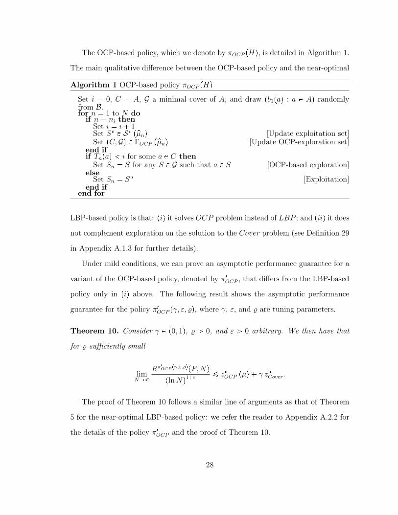
The OCP-based policy, which we denote by πOCP pHq, is detailed in Algorithm 1.

The main qualitative difference between the OCP-based policy and the near-optimal

Algorithm 1 OCP-based policy πOCP pHq

Set i 0, C A, G a minimal cover of A, and draw pb1paq : a P Aq randomlyfrom B.for n 1 to N do

if n ni thenSet i i 1Set S P S ppµnq [Update exploitation set]Set pC,Gq P ΓOCP ppµnq [Update OCP-exploration set]

end ifif Tnpaq i for some a P C then

Set Sn S for any S P G such that a P S [OCP-based exploration]else

Set Sn S [Exploitation]end if

end for

LBP-based policy is that: piq it solves OCP problem instead of LBP ; and piiq it does

not complement exploration on the solution to the Cover problem (see Definition 29

in Appendix A.1.3 for further details).

Under mild conditions, we can prove an asymptotic performance guarantee for a

variant of the OCP-based policy, denoted by π1OCP , that differs from the LBP-based

policy only in piq above. The following result shows the asymptotic performance

guarantee for the policy π1OCP pγ, ε, %q, where γ, ε, and % are tuning parameters.

Theorem 10. Consider γ P p0, 1q, % ¡ 0, and ε ¡ 0 arbitrary. We then have that

for % sufficiently small

limNÑ8

Rπ1OCP pγ,ε,%qpF,Nq

plnNq1ε¤ zOCP pµq γ zCover.

The proof of Theorem 10 follows a similar line of arguments as that of Theorem

5 for the near-optimal LBP-based policy: we refer the reader to Appendix A.2.2 for

the details of the policy π1OCP and the proof of Theorem 10.

28

2.6 Computational Aspects for Solving OCP and Policy Implemen-tation

In this section we address the computational aspects for the practical implementation

of the OCP-based policy. We provide strong evidence that, for a large class of

combinatorial problems, our policies scale reasonably well. For this, we focus our

attention on the practical solvability of OCP , which our policies solve repeatedly

over time. Note that Combpq and OCP pq have generic combinatorial structures

and hence are, a priori, theoretically hard to solve. Hence, practical tractability of

said problems is essential for implementation.

Note that the OCP-based policy solves OCP at an exponentially decreasing fre-

quency, thus ensuring its timely solvability in the long run. In the short run, a

time-asynchronous version of the policy, that uses the incumbent solution to OCP

until the new solution becomes available, can be implemented (see Appendix A.3.6).

As mentioned above, in generalOCP might be theoretically intractable. Nonethe-

less, in Appendix A.3.7 we present a greedy oracle polynomial-time heuristic for

OCP . The greedy heuristic requires a polynomial number of calls to an oracle for

solving Comb. It therefore runs in polynomial time when Comb is polynomially solv-

able. Furthermore, it provides a practical solution method for OCP when Comb is

not expected to be solvable in polynomial time, but is frequently tractable in practice

(e.g., medium-size instances of NP-complete problems such as the traveling salesman

(Applegate et al., 2011), Steiner tree (Magnanti and Wolsey, 1995; Koch and Martin,

1998; Carvajal et al., 2013), and set cover problems (Etcheberry, 1977; Hoffman and

Padberg, 1993; Balas and Carrera, 1996)).

An advantage of the greedy heuristic described in Appendix A.3.7 is that it only

requires an oracle for solving Comb and hence does not require any knowledge of the

specific structure of Comb. In Section 2.7 we implement a variant of the OCP-based

29

policy that uses this greedy heuristic to solve OCP . We show that even such a

myopic approach can already provide a reasonable approximation of the OCP-based

policy and can significantly outperform alternative approaches. However, we would

expect much better performance from heuristics or approximations that exploit the

particular structure of Comb for a specific class of problems. Such focus on a specific

class of problems is, however, beyond the scope of this paper, thus we instead use

mixed-integer programming (MIP) to exploit structure in a generic way.

Over 50 years of theoretical and computational developments in MIP (Junger

et al., 2010) have led to state-of-the-art MIP solvers with machine-independent

speeds that nearly double every year (Achterberg and Wunderling, 2013; Bixby,

2012). One key to this speed is a wide range of highly effective generic primal

heuristics (e.g., see Fischetti and Lodi (2011) and the “Primal Heuristic” sections

of Gamrath et al. (2016); Maher et al. (2017), and Gleixner et al. (2017)). Hence,

formulating OCP as a MIP opens up a wide range of exact and heuristic algorithms

to solve it. However, the effectiveness of this approach is strongly contingent on

constructing a formulation with favorable properties (Vielma, 2015). In what follows

we focus our attention on constructing such formulations for the case in which Comb

is theoretically tractable, i.e., it is solvable in polynomial time. This class includes

problems such as shortest path, network flow, matching, and spanning tree problems

(Schrijver, 2003). For these problems we develop polynomial-sized MIP formulations

of OCP , which can be effectively tackled by state-of-the-art solvers.

2.6.1 MIP Formulations of OCP for Polynomially-Solvable Problems

In this section we assume that Comb is polynomially solvable. However, this does

not imply that OCP is tractable or practically solvable, as it might contain an

exponential (in |A|) number of variables and constraints. The following theorem,

whose proof can be found in Appendix A.3.1, ensures that OCP remains in NP,

30

the class of non-deterministic polynomially-solvable problems (see e.g., Cook et al.

(1998)).

Theorem 11. If Comb is in P, then OCP is in NP.

While it is possible to establish a non-trivial jump in theoretical complexity for

problems within P, we deem the study of the theoretical complexity of OCP for

different problems outside the scope of the paper. Instead, here we focus on their

practical solvability. For this, we first establish the existence of polynomial-sized MIP

formulations when Comb admits a linear programming (LP) formulation. Then, we

address the case when Comb admits a polynomial-sized extended LP formulation,

and finally, the case when Comb does not admit such an extended formulation.

Problems with LP Formulations. We present a polynomial-sized formulation

of OCP when Comb admits a polynomial-sized LP formulation. To describe this

formulation in simple matrix notation we assume that A : t1, . . . , |A|u. Moreover,

for v P Rr, let diagpvq be the r r diagonal matrix with v as its diagonal. Also, we

remember that l plpaq : a P Aq is the vector of lower bounds on the range of F .

Proposition 12. Let yS P t0, 1u|A| be the incidence vector of S P S, M P Rm|A|,

and d P Rm be such that yS(SPS

!y P t0, 1u|A| : My ¤ d

)and conv

yS(SPS

31

y P r0, 1s|A| : My ¤ d

(. Then a MIP formulation of OCP pνq is given by

min¸iPA

¸aPA

νpaqyipaq zCombpνq

(2.8a)

s.t. xpaq ¤¸iPA

yipaq, a P A (2.8b)

Myi ¤ d, i P A (2.8c)

MTw ¤ diagplqp1 xq diagpνqx (2.8d)

dTw ¥ zComb pνq (2.8e)

xpaq, yipaq P t0, 1u , w P Rm, a, i P A, (2.8f)

where x pxpaq : a P Aq, yi pyipaq : a P Aq, and 1 is a vector of ones.

In the above, x represents the incidence vector of a critical set. Such a condition

is imposed via LP duality, using constraints (2.8d) and (2.8e), and eliminates the

necessity of introducing constraint (2.7c) for each solution in S. Similarly, each yi

represents the incidence vector of a solution S P S. A formal proof of the validity of

this formulation is included in Appendix A.3.3.

Formulation (2.8) has Op|A|2q variables and O pm |A|q constraints. If m is poly-

nomial in the size of the input of Comb, then we should be able to solve (2.8) directly

with a state-of-the-art integer programming (IP) solver. If m is exponential, but the

constraints in the LP formulation can be separated effectively, we should still be able

to effectively deal with (2.8c) within a branch-and-cut algorithm. However, in such a

case one would have an exponential number of w variables, which would force us to

use a more intricate, and potentially less effective, branch-and-cut-and-price proce-

dure. Nonetheless, when Comb does not admit a polynomial-sized LP formulation,

one can still provide formulations with a polynomial number of variables, many of

them also having a polynomial number of constraints. We discuss such cases next.

32

Problems with Polynomial-Sized Extended Formulations. The first way to

construct polynomial-sized IP formulations of OCP is to exploit the fact that many

polynomially-solvable problems with LP formulations with an exponential number

of constraints also have polynomial-sized extended LP formulations (i.e., formula-

tions that use a polynomial number of auxiliary variables). A standard example

of this class of problems is the spanning tree problem, where m in the LP for-

mulation required by Proposition 12 is exponential in the number of nodes of the

underlying graph. However, in the case of spanning trees, we can additionally use

a known polynomial-sized extended formulation of the form P : ty P r0, 1s|A| :

D z P Rp, Cy Dz ¤ du where C P Rm1|A|, D P Rm1p and d P Rm1, with

both m1 and p being only cubic on the number of nodes (and hence polynomial in

|A|) (Martin, 1991, e.g.). This formulation satisfies yS(SPS P X t0, 1u|A| and

conv yS(SPS

P . Then, a MIP formulation with a polynomial number of vari-

ables and constraints of OCP for the spanning tree problem is obtained by replacing

(2.8c) with Cyi Dzi ¤ d, replacing (2.8d) with CTw ¤ diagplqp1 xq diagpνqx

and DTw ¤ 0, and adding the polynomial number of variables zi for i P t1, . . . , |A|u.

Similar techniques can be used to construct polynomial-sized formulations for other

problems with polynomial-sized extended LP formulations.

Problems without Polynomial-Sized Extended Formulations. It has re-

cently been shown that there is no polynomial-sized extended LP formulations for

the non-bipartite perfect matching problem (Rothvoß, 2017). Hence, we cannot

use the techniques in the previous paragraph to construct polynomial-sized IP for-

mulations of OCP for matching. Fortunately, a simple linear programming obser-

vation and a result by Ventura and Eisenbrand (2003) allow constructing a ver-

sion of (2.8) with a polynomial number of variables. The observation is that a

solution y is optimal for max νTy : My ¤ d

(if and only if it is optimal for

33

max νTy : MT

i y ¤ di @i P I pyq(

where I pyq : i P t1, . . . ,mu : MT

i y di

(is the set of active constraints at y, and Mi is the i-th row of M . The number of

active constraints can still be exponential for matching. However, for each perfect

matching y, Ventura and Eisenbrand (2003) give explicit C P Rm1|A|, D P Rm1p

and d P Rm1, such that m1 and p are polynomial in |A| and ty P r0, 1s|A| : D z P

Rp, Cy Dz ¤ du ty P R|A| : MTi y ¤ di @i P I pyqu. Using these matrices

and vectors we can then do a replacement of (2.8d) analog to that for spanning trees

to obtain a version of (2.8) with a polynomial number of variables. We would still

have an exponential number of constraints in (2.8c), but these can be separated in

polynomial time for matching, so OCP for matching could be effectively solved by

branch-and-cut.

Perfect matching is the only explicit polynomially-solvable combinatorial opti-

mization problem that is known not to admit a polynomial-sized extended LP for-

mulation. However, Rothvoß (2013) shows that there must exist a family of matroid

problems without a polynomial-sized extended LP formulation. Fortunately, it can

be shown (e.g., see Lemma 32 in Appendix A.3.2) that for matroid problems, there

is a unique critical set C A that can be found in polynomial time. Once this set

is obtained, we can simply replace (2.8b) by 1 ¤°iPA y

ipaq for all a P C and remove

(2.8d)–(2.8e). We are not aware of any other polynomially-solvable combinatorial

optimization problem which requires non-trivial results to formulate OCP with a

polynomial number of variables.

Remark 4. Further improvements and extensions to (2.8) can be achieved. We

give two such examples in Appendices A.3.4 and A.3.5. The first example shows

how (2.8) for OCP can be extended to the case when Comb is not in P, but admits

a compact IP formulation. The second example gives a linear-sized formulation of

OCP for shortest path problems.

34

2.7 Numerical Experiments

In this section we study the finite-time performance of the OCP-based policy from

Section 2.5. In particular, we consider two policies: the OCP-based policy (as defined

in Algorithm 1), and a variant that solves OCP heuristically in a greedy way (using

Algorithm 5 presented in Appendix A.3.7). We refer to this latter policy as the

Greedy-Heuristic policy. We divide the numerical experiments into two classes: long-

term and short-term experiments. For each class of experiments, we first describe

the benchmark policies and then discuss the settings studied.

2.7.1 Long-Term Experiments

Benchmark Policies and Implementation Details

Benchmark Policies. Our benchmark policies are versions of UCB1 (Auer et al.,

2002), adapted to improve performance in the combinatorial setting. The UCB1

policy implements solution Sn in period n, where

Sn P argminSPS

#°m n:SmS

°aPS bmpaq

|m n : Sm S|

d2 lnpn 1q

|m n : Sm S|

+.

Note that the estimate cost for solution S is based solely on past implementations

of that solution. We improve performance of UCB1 by: piq conducting parameter

estimation at the ground element level to reduce variance of estimation; piiq using

min tTnpaq : a P Su instead of |m n : Sm S| to adjust confidence interval length

to better reflect the amount of information used in estimating parameters; piiiq

adjusting said length so that confidence bounds remain within the bounds implied

by the range of F ; and pivq reducing the solution set so that it only includes solutions

that are minimal with respect to inclusion – this could improve performance by

preventing UCB1 to implement solutions that are clearly suboptimal. The resulting

35

policy, which we denote UCB1+, implements solution Sn in period n, where

Sn P argminSPS

#max

#¸aPS

pµnpaq d

2 lnpn 1q

min tTnpaq : a P Su,¸aPS

lpaq

++.

In a similar setting, Gai et al. (2012) propose an alternative adaptation of UCB1: a

modified version of such a policy in period n implements

Sn P argminSPS

#¸aPS

max

#pµnpaq dpK 1q lnpn 1q

Tnpaq, lpaq

++,

for a tuning parameter K ¡ 0. We denote this policy as Extended UCB1+.

Remark 5. Note that computing Sn in Extended UCB1+ can be accomplish by

solving an instance of Combpq. Implementing UCB1+ in contrast, requires solving

for Sn via explicit enumeration.

Implementation Details. We report results when the marginal distributions of F

are exponential (we normalize the mean cost vector so that the maximum solution

cost is at most one): we tested many cost distributions and observed consistent

performance. For the OCP-based and Greedy-Heuristic policies, we report the results

for H 5: preliminary tests using H P t5, 10, 20u always resulted in logarithmic

regrets. When choosing a solution from the exploration set to implement, in case

of a tie, our proposed policies select the solution that contains the most number of

critical elements. In case of a second tie, they select a solution with the smallest

average cost. We implemented UCB1+ and Extended UCB1+ with and without

truncating indices at the implied lower bounds. Here, we present the point-wise

minimum regret among both versions of each policy. We set K 1 in Extended

UCB1+, as this selection outperformed the recommendation in Gai et al. (2012),

and also is the natural choice for extending the UCB1 policy. Finally, all policies

36

start with an initialization phase in which each solution in a common minimum-size

cover of A is implemented.

All figures in this section report average performance for N 2000 over 100

replications, and dotted lines represent 95% confidence intervals. All policies were

implemented in MATLAB R2011b. Shortest path problems were solved using Dijk-

stra’s algorithm except when implementing UCB1+ (note that because of the index

computation, the optimization problem must be solved by enumeration). For Steiner

tree and knapsack problems, we solved standard IP formulations using GUROBI 5.0

Optimizer. The OCP-based policy solves formulation (2.7) of OCP using GUROBI

5.0 Optimizer. All experiments ran on a machine with an Intel(R) Xeon(R) 2.80GHz

CPU and 16GB of memory. The average running time for a single replication was

around 30 seconds for the UCB1+, Extended UCB1+ and Greedy-Heuristic poli-

cies, and around 1.5 minutes for the OCP-based policy. (Note, however, that while

the running time of the OCP-based policy grows (roughly) logarithmically with the

horizon, those of UCB1+ and Extended UCB1+ grow linearly.)

Settings and Results

We present settings complementary to those in Examples 1 and 2 in the sense that

critical sets are large, thus the OCP-based and Greedy-Heuristic policies do not

have an immediate advantage. (See Appendix A.4 for numerical experiments on

Examples 1 and 2.) The settings are comprised of the shortest path, Steiner tree

and knapsack problems. We observed consistent performance of our policies across

these settings: here we only show a representative from each class.

Shortest Path Problem. We consider a shortest path problem on a randomly

generated layered graph – see panel (a) of Figure 2 in Ryzhov and Powell (2011) for

an example of a layered graph. The graph consists of a source node, a destination

node, and 5 layers in between, each containing 4 nodes. In each layer, every node (but

37

those in the last layer) is connected to 3 randomly chosen nodes in the next layer.

The source node is connected to every node in the first layer and every node in the

last layer is connected to the destination node. Mean arc costs are selected randomly

from the set t0.1, 0.2, . . . , 1u and then normalized. The representative graph is such

that |A| 56, |S| 324, and while the minimum-size cover of A is of size 13, the

solution-cover to OCP pµq is of size 16 with an implied critical set of size 40.

Knapsack Problem. Here the set A represents items that might go into the knap-

sack to maximize total utility. The solution set S consists of the subsets of items

whose total weights do not exceed the knapsack weight limit. Weight and utility of

items, as well as the weight limit, are selected randomly. The representative setting

is such that |A| 20, |S| 24680, the minimum-size cover is of size 4, and the

solution-cover to OCP pµq is of size 8 with an implied critical set of size 17.

Minimum Steiner Tree Problem. We consider a generalized version of the Steiner

tree problem (Williamson and Shmoys, 2011), where for a given undirected graph

with non-negative edge costs and a set of pairs of vertices, the objective is to find

a minimum-cost subset of edges (tree) such that every given pair is connected in

the set of selected edges. The graphs as well as the pairs of vertices are generated

randomly, as well as the mean cost values. The representative setting is such that

|A| 18, |S| 10651, the minimum-size cover is of size 2. We consider two settings:

one where the lower bound vector is l 0 (the solution-cover to OCP pµq is of size

7 and the critical set is of size 17) and one where lower bounds are positive numbers

that are selected randomly (the solution-cover to OCP pµq is of size 5 and the critical

set is of size 12).

Results. The left and right panel in Figure 2.2 depict the average performance of

different policies for the shortest path and knapsack settings, respectively. We see

that in both settings, the OCP-based and Greedy-Heuristic policies significantly out-

perform the benchmark. The left panel in Figure 2.3 depicts the average performance

38

N100 600 1100 1600 2000

Reg

ret

50

100

150

200

250

300Extended

UCB1+UCB1+

Greedy-Heuristic

OCP-based

N100 600 1100 1600 2000

Reg

ret

5

10

15

20

25

30

UCB1+

Greedy-Heuristic

Extended UCB1+

OCP-based

Figure 2.2: Average performance of different policies on the representative settingfor the shortest path (left) and knapsack (right) problems.

N100 600 1100 1600 2000

Reg

ret

20

40

60

80

100

Extended UCB1+

UCB1+

Greedy-Heuristic

OCP-based

N100 600 1100 1600 2000

Reg

ret

10

20

30Extended

UCB1+

UCB1+

Greedy-Heuristic

OCP-based

Figure 2.3: Average performance of different policies on the representative settingfor the Steiner tree problem with zero (left) and positive (right) lower bounds.

of different policies for the Steiner tree setting when all cost lower bounds are set to

zero. In this case, all arcs (but those trivially suboptimal) are critical, however, the

OCP-based and Greedy-Heuristic policies still outperform the benchmark. The right

panel in Figure 2.3 depicts average performance in the setting where lower bounds

are positive numbers. Note that the OCP-based policy significantly outperforms the

benchmark as it successfully limits exploration to a critical set. Also note that the

non-concave behavior of the regret curve of UCB1+ arises only in the transient as a

by-product of truncation, and it disappears at around n 1200.

Sample Path Regret Comparison. The results in this section show that the

39

average performance of our policies is significantly better than that for the bench-

mark. It turns out that our policies outperform the benchmark not only in terms of

average, but also in terms of worst-case regret: we compared the sample path final

regrets (i.e., at time period N 2000) of OCP-based policy with those of UCB1+

and Extended UCB1+ policies: out of 700 sample paths in the numerical experi-

ments in Section 2.7.1 (and including those in the Appendix A.4), the OCP-based

policy outperforms the UCB1+ and Extended UCB1+ policies in all 700 (i.e., 100%

of sample paths) and 697 (i.e., 99.6% of sample paths), respectively.

2.7.2 Experiment with Size of the Ground Set

In Section 2.1 we argued that, in the combinatorial setting, it is the constant ac-

companying the lnN term in a performance guarantee that is worth characterizing.

However, prior work (see Section 2.2), lacking a fundamental performance limit, in-

stead writes such an accompanying constant as a function of the size of the ground

set (i.e., |A|). However, following Theorem 5, we know that such a constant is not

a trivial function of |A|. Thus, the question of how said constant scales in practice

with the size of the underlying combinatorial problem is of much relevance. For this

reason, we next explore how performance of various policies varies with the size of

the ground set.

We experiment with the shortest path problem on a layered graph (see Section

2.7.1 for a description) with L layers, 2 nodes in each layer, complete connections

between layers, and a direct arc from the source s to sink t. We experiment with

L 2, 4, 6, 8, 10 which results in |A| 9, 17, 25, 33, 41 and |S| 5, 17, 65, 257, 1025,

respectively.

We add a direct s t arc (path) to the original description of the layered graph

so as to isolate the effect of size of the ground set on the performance of different

policies. To this end, we let the expected cost of the s t arc (path) be 0.1, while

40

all other arcs have an expected cost of 0.2pL 1q where L is the number of layers.

Therefore, the s t path is the expected shortest path while all other paths (each of

which has L1 arcs) have an expected cost of 0.2, regardless of the size of the ground

set. Thus, increasing the size of the ground set does not affect the cost (regret) of

different paths in different instances. We run the experiments for N 20000 and 40

replications.

For the OCP-based policy, we solve the OCP problem using the linear-sized for-

mulation (A.22) presented in the Appendix A.3.5. We observe a behavior similar to

the graph on the left panel of Figure 2.5 for all choices of L. That is, the cumula-

tive regret of all three policies grow similar to a function K lnpnq for some policy-

dependent constant K. We consider two estimates for such a constant: (i) KFinal,

which we find by dividing the average final regret, which we denote by Rp20000q, by

lnp20000q, that is, KFinal : Rp20000q lnp20000q; piiq KLS, which is found by fitting

the function KLS lnpnq to the sample of average regrets for n 100, 200, . . . , 20000

(by minimizing the sum of squared errors). We present the value of both constants

for the three policies and varying |A| in Figure 2.4. We also present the average

performance and computation time of different policies for the instance with L 10

(|A| 41 and |S| 1025) as a representative setting in Figure 2.5 as we observed

similar behavior in other instances. As can be seen in the left panel of Figure 2.5

(and also from Figure 2.4), the OCP-based policy significantly outperforms both

benchmark policies regardless of the size of the ground set. Moreover, the constants

KLS and KFinal are significantly smaller for the OCP-based policy than those for the

benchmark policies. In addition, such constants grow with a much smaller rate for

the OCP-based policy than the benchmarks. Moreover, as illustrated by the right

panel of Figure 2.5, the computation time of the OCP-based policy grows logarithmi-

cally with N . Furthermore, there is a significant variation if we consider computation

times. This is shown in Table 2.1, which presents the average running time for a com-

41

|A|9 17 25 33 41

KLS

0

20

40

60

80

100

120

|A|9 17 25 33 41

KF

inal

0

50

100

150

200

Extended UCB1+

OCP-based

Extended UCB1+

UCB1+

OCP-based

UCB1+

Figure 2.4: Constants KLS (left) and KFinal (right) when increasing the size of theground set.

N #1040.5 1 1.5 2

Reg

ret

0

200

400

600

800

1000

OCP-based

UCB1+

Extended UCB1+

N #1040.5 1 1.5 2

Cum

ulat

ive

Com

puta

tion

Tim

e

0

100

200

300

400

UCB1+

Extended UCB1+

OCP-based

Figure 2.5: Average performance (left) and computation time (right) as a functionof N for the instance with L 10, |A| 41, and |S| 1025.

plete replication for each policy. This time includes all calculations required by the

policy (e.g., for the OCP-based policy, it includes the solution time of all instances

of OCP and Comb as dictated by Algorithm 1). We can see that the OCP-based

Table 2.1: Average total computation time (in seconds) for each replication of N 20000. |A|

9 17 25 33 41

OCP 75.54 79.43 81.18 92.60 142.38UCB1+ 65.47 127.38 376.56 1483.71 6686.70

Extended UCB1+ 103.59 190.64 267.22 342.93 418.83

policy runs faster than both benchmark policies for (almost) all instances (we note

42

that although for much larger instances, one expects the Extended UCB1+ to run

faster than the OCP-based policy, the Extended UCB1+ performs very poorly, in

terms of regret, regardless of the size of the instance). Moreover, UCB1+, which is

the more “competitive” benchmark policy in terms of performance, is significantly

slower than the OCP-based policy. These observations further pronounce the prac-

tical advantage of the OCP-based policy both in terms of performance (i.e., regret)

and computation time.

2.7.3 Short-Term Experiments

Benchmark Policies and Implementation Details

Benchmark Policies. Our benchmark policies are adaptations of the Knowledge-

Gradient (KG) policy in Ryzhov et al. (2012) and the Gittins index approximation in

Lai (1987) to our setting. Both policies require prior knowledge of the time horizon

N , and because of this, several runs of the benchmark policies are necessary to

construct their cumulative regret curves.

The KG policy requires a prior distribution for the cost and hyper-parameters.

In our implementation, we use the Exponential-Gamma conjugate prior for each

ground element. That is, the algorithm assumes that for each a P A, Bpaq follows an

exponential distribution with rate µpaq, but this rate itself is random, and initially

distributed according to a Gamma distribution with parameters αa,0 and βa,0. At

period n, the posterior distribution of µpaq is a Gamma with parameters

αa,n αa,0 Tnpaq, βa,n βa,0 ¸

m n:aPSmbmpaq, a P A.

Thus at period n, the KG algorithm implements solution SKGn , where

SKGn P argminSPS

#¸aPS

βa,nαa,n 1

pN nq EnS

#minS1PS

#¸aPS1

βa,nαa,n 1

+ minS1PS

#¸aPS1

βa,n1

αa,n1 1

+++,

43

where the expectation is taken with respect to Bn. The expectation above cor-

responds to the knowledge gradient term vKG,nS in the notation of Ryzhov et al.

(2012). Unlike in that paper, there is no closed-form expression for vKG,nS in our set-

ting. Our plain vanilla implementation of the KG algorithm computes such a term

via Monte Carlo simulation, and performs the outer minimization via enumeration.

The complexity of the implementation limited the size of the settings we tested.

The second benchmark is an approximation based on the Gittins index rule which

in the finite-horizon undiscounted settings takes the form of an average productivity

index (see Nino-Mora (2011)), and although it is not optimal in general, it is still

applied heuristically. Our implementation assigns an index to each ground element,

and computes the index of a solution as the sum of the indexes of the ground ele-

ments included in that solution. The policy requires a parametric representation of

the uncertainty. To mimic a setting where the functional form of the cost distribu-

tions is unknown, we consider the approximation in Lai (1987) based on normally

distributed costs and use Normal/Normal-Gamma conjugate priors (this is motivated

by a central limit argument): in our approximation, the index of a ground element

a P A at period n is given by

gan,Npµa,n, λa,n, αa,n, βa,nq

µa,n

dβa,n

pαa,n 1qλa,nh

λa,n λa,0

N n 1 λa,n λa,0

,

where µa,n and λa,n are the mean and variance of the normal posterior, respectively,

αa,n and βa,n are the hyper-parameters of the Gamma posterior, respectively, and

hpq approximates the boundary of an underlying optimal stopping problem. The

policy implements solution SGittn , where

SGittn P argminSPS

#¸aPS

gan,Npµa,n, λa,n, αa,n, βa,nq

+.

Implementation Details. The implementation details are as in the long-term

44

experiments. The average running time for a single replication ranged from around

one second for the OCP-based policy to around 2 seconds for Gittins to less than

10 minutes for KG. We exclude the results for the UCB1+ and Extended UCB1+

policies, because they were consistently outperformed by the OCP-based policy.

Settings and Results

We consider randomly generated (structure and costs) settings of shortest path,

Steiner tree and knapsack problems. We observed consistent performance of the

policies across settings, and show only a representative setting for each class of prob-

lems. There, the total number of periods is selected so as to visualize the value at

which the OCP-based policy begins outperforming the benchmark. In all settings,

the benchmark policies initially provide a better performance compared to the OCP-

based policy, but the latter policy eventually surpasses the benchmarks for moderate

values of N . The same holds true for the case of the Greedy-Heuristic policy.

Shortest Path Problem. The left panel at Figure 2.6 depicts the average perfor-

mances for a shortest path problem in a layered graph with 5 layers, each with 4

nodes, and 2 connections between each inner layer. The representative setting is such

that |A| 40, |S| 64, the minimum-size cover is of size 9, and the solution-cover

to OCP pµq is of size 10 with an implied critical set of size 23.

Minimum Steiner Tree Problem. The central panel at Figure 2.6 depicts the

average performances on a representative setting for the Steiner tree problem. The

representative setting is such that |A| 9, |S| 50, the minimum-size cover is of

size 2, and the solution-cover to OCP pµq is of size 4 with an implied critical set of

size 8.

Knapsack Problem. The right panel at Figure 2.6 depicts the average perfor-

mances on a representative setting for the knapsack problem. (Here we report on

the average behavior over 500 replications so that the confidence intervals do not

45

cross.) The representative setting is such that |A| 11, |S| 50, the minimum-size

cover is of size 7, and the solution-cover to OCP pµq is of size 2 with an implied

critical set of size 5.

N40 100 160 220 280 340 400

Reg

ret

13

26

39

52

65

OCP-based

Gittins

KG

Greedy-Heuristic

N10 30 50 70 90100

Reg

ret

1

2

3

Greedy-Heuristic

Gittins

KG

OCP-based

N10 30 50 70 90 110

Reg

ret

4.5

5

5.5

OCP-based

Greedy-Heuristic

KG

Gittins

Figure 2.6: Average performance of different policies on the representative settingfor the shortest path (left), Steiner tree (center) and knapsack (right) problems – thevertical lines show the 95% confidence intervals.

2.8 Conclusion

In this paper we study a class of sequential decision-making problems where the

underlying single-period decision problem is a combinatorial optimization problem,

and there is initial uncertainty about its objective coefficients. By framing the prob-

lem as a combinatorial multi-armed bandit, we adapt key ideas behind results in the

classical bandit setting to develop efficient practical policies. We show that in addi-

tion to answering the question of when (with what frequency) to explore, which is

key in the traditional bandit setting, in the combinatorial setting the key questions

to answer are what and how to explore. We answer such questions by solving an

optimization problem which we call the Lower Bound Problem (LBP). We establish

a fundamental limit on the asymptotic performance of any admissible policy that

is proportional to the optimal objective value of the LBP problem. We show that

such a lower bound might be asymptotically attained by near-optimal policies that

46

adaptively reconstruct and solve LBP at an exponentially decreasing frequency. Be-

cause LBP is likely intractable in practice, we propose a simpler and more practical

policy, namely the OCP-based policy, that instead reconstructs and solves a proxy

for LBP, which we call the Optimaltiy Cover Problem (OCP). This proxy explicitly

solves for the cheapest optimality guarantee for the optimal solution to the under-

lying combinatorial problem. We prove a performance guarantee for a variant of

the OCP-based policy, which is proportional to the optimal objective value of the

OCP and can be compared to that of LBP. We also provide strong evidence of the

practical tractability of OCP which in turn implies that the proposed OCP-based

policies are scalable and implementable in real-time. Moreover, we test performance

of the proposed policies through extensive numerical experiments and show that they

significantly outperform relevant benchmark in the long-term and are competitive in

the short-term.

The flexibility of the OCP-based policies allows them to be easily extended or

combined with other techniques that consider similar what-and-how-to-explore ques-

tions. For instance, the OCP-based policy can be easily combined with the “barycen-

tric spanner” of Awerbuch and Kleinberg (2004) to extend our results from element-

level observations to set- or solution-level observations. Indeed, it can be shown that

in such feedback settings, efficient exploration amounts to focus exploration on the

solution to a variant of OCP. Moreover, the performance guarantee in Theorem 10

would remain valid with the constants associated with this alternative formulation.

See Appendix A.5 for further details.

From our results, we observe a performance gap between the fundamental limit on

(asymptotic) performance (Theorem 5) and the upper bound on the regret associated

with near-optimal policies (Theorem 6). Although we provide a detailed discussion

of this gap in Appendix A.1.5, future research can further investigate the possibility

of closing this gap. Moreover, relaxing some of the assumptions in this work (e.g.,

47

considering unbounded cost distributions with heavy tails) could introduce additional

interesting challenges. Furthermore, studying combinatorial bandit settings with

non-linear objective functions is another direction for future research.

48

3

A Dynamic Clustering Approach to Data-DrivenAssortment Personalization

3.1 Introduction

Motivation and Objective. According to a recent study by eMarketer (eMarketer

2017), worldwide business-to-consumer e-commerce sales will reach more than $4

trillion in 2020. With the rapid growth of online sales, retailers are finding unprece-

dented opportunities to both enhance the customer experience and increase revenue.

A customer-centric practice that is becoming increasingly pervasive in online retail-

ing is assortment personalization. This is the practice of offering a product mix that

is tailored to each customer’s taste based on previously collected data (Arora et al.

2008). The benefits of personalization are twofold: on one hand, it results in higher

revenue for the retailer due to the increase in sales that results from providing cus-

tomers with a set of products that more accurately matches their preferences (Arora

et al. 2008); on the other hand, it attracts customer attention and fosters customer

loyalty and satisfaction (Ansari and Mela 2003).

There are numerous examples of personalization in online retailing. For example,

49

Amazon.com uses collaborative filtering to personalize recommendations to its users

(Linden et al. 2003; Arora et al. 2008). A recent New York Times article reviews a

growing number of start-ups that are investing in highly personalized online shopping

technology (Wood 2014). Among these start-ups is Stitch Fix, an online personalized

clothing service that periodically sends its customers boxes containing five pieces of

clothing based on each customer’s taste (e.g., size, favorite brand and color, budget).

Trunk Club is another personalized clothing service.

As noted in the New York Times article, in personalized shopping “the magic

comes from data.” Online retailers collect an abundance of customer data (e.g., de-

mographic, transactional, etc.). However, given the broad range of customer profiles,

collecting a sufficient amount of transaction data on each customer profile may not

be possible. This, in turn, limits the retailer’s ability to accurately estimate prefer-

ences and offer personalized assortments. The goal of this paper is to explore the

efficient use of data for assortment personalization in online retailing.

Model. We consider an online retailer that sells multiple products over a finite

selling season. Customers arrive sequentially and the retailer offers each customer

an assortment of products. The retailer may face display or capacity constraints that

limit the number of products in the offered assortment. The customer then decides

whether or not to make a purchase. The retailer’s objective is to maximize expected

cumulative revenue over the selling season.

Customers are divided into different profiles according to their observable at-

tributes, such as demographic profiles (e.g., gender, age, location) and past trans-

action information (e.g., purchase history, payment method). This information is

exogenous and available upon arrival via the customer’s login information or inter-

net cookies. We assume that, from the perspective of the retailer, customers with a

common profile are homogeneous with respect to their product preferences (in prac-

50

tice, the definition of profiles reflects the degree of customer information available

to the retailer and the level of granularity that allows the retailer to operationalize

other marketing decisions).

A central assumption in this work is that the retailer has limited prior information

on customers’ preferences. Personalizing assortments thus requires the estimation of

such preferences which, in turn, requires observing the customers’ purchasing deci-

sions (that are themselves affected by the retailer’s assortment decisions). This gives

rise to an exploration (learning preferences) versus exploitation (earning revenue)

trade-off. As such, we formulate the assortment selection problem as a multi-armed

bandit problem (Thompson 1933; Robbins 1985) with multiple simultaneous plays:

each product represents an arm and including a product in the offered assortment is

equivalent to pulling that arm – see Caro and Gallien (2007).

Off-the-shelf bandit approaches to the assortment problem call for solving an in-

dependent instance for each customer profile. However, practical instances of the

problem might have scores of different profiles. This implies that arriving to rea-

sonable preference estimates for a given profile might take an unreasonably large

amount of time. More importantly, such an approach ignores the possibility that

customers with different profiles may share similar product preferences. In this pa-

per, we show that the retailer can exploit these similarities by pooling information

across customers with similar purchasing behavior. To that end, we consider the

existence of an underlying mapping of profiles to clusters, where a cluster is defined

as a set of customer profiles with the same product preferences. This mapping is

initially unknown to the retailer.

We propose a dynamic clustering policy under which the retailer estimates both

the underlying mapping of profiles to clusters and the preferences of each cluster.

Assortment decisions are based on the estimated mapping by adapting decision rules

from traditional bandit algorithms. We use a Bayesian framework, called the Dirich-

51

let Process Mixture model, to represent uncertainty about the mapping of profiles

to clusters. This model arises as a natural selection given the discrete nature of the

mapping and allows us to draw inference without having to predetermine the number

of clusters upfront. The dynamic clustering policy estimates the mapping of profiles

to clusters as well as the preference parameters for each cluster by using a Markov

Chain Monte Carlo (MCMC) sampling scheme.

Main Contributions. The contributions of this paper are as follows:

We propose a prescriptive approach, called the dynamic clustering policy, for as-

sortment personalization in an online setting. The proposed policy combines existing

tools from the Bayesian data analysis literature (for estimating customer preferences

through dynamic clustering) and from the machine learning / operations manage-

ment literature (to prescribe personalized assortment decisions). This approach is

motivated by the retailers’ interest in identifying clusters of customers with similar

preferences and in offering personalized assortments to their customers. Unlike most

existing work that focuses on offline settings (i.e., using historical data), we propose

an online tool for assortment personalization that can be implemented in real-time.

Moreover, the proposed dynamic clustering policy is fairly general and flexible as the

number of clusters (segments) is endogenous and does not need to be predetermined.

We illustrate the practical value of the dynamic clustering policy in a realistic

setting by using a dataset from a large Chilean retailer. We use the case study to

quantify the efficiency and demonstrate the implementability of the dynamic clus-

tering policy. The dataset consists of roughly 95,000 customer-tied click records in

the retailer’s website for 19 products in the footwear category. We contrast the per-

formance of the proposed policy to that of a data-intensive policy that ignores any

potential similarity in preferences across profiles and thus estimates product prefer-

ences for each profile separately. We find that, under the MNL model, the proposed

52

policy generates more than 37% additional transactions (on average) compared to the

data-intensive policy in the case study. This finding quantifies the potential benefit

of leveraging similarity in customer preferences by adaptively pooling information

across profiles with similar purchasing behavior to expedite the learning process.

The performance of the dynamic clustering policy is remarkable, considering that

the underlying customer population in the case study is rather heterogeneous. We

also compare the performance of the proposed policy to that of a linear-utility pol-

icy that assumes a more structured model of customer preferences. In particular,

the linear-utility policy assumes that demand is driven by an MNL choice model in

which mean utilities are linear functions of customer attributes. The findings from

the case study show that the proposed policy generates more than 27% additional

transactions (on average) compared to the linear-utility policy under the MNL de-

mand model. While this can be partially explained by the fact that preferences in

the dataset do not exhibit a linear structure, the advantage of the dynamic cluster-

ing policy persists even when using synthetic data (generated based on the dataset)

under which mean utilities are linear functions of customer attributes by construc-

tion. This finding reinforces the benefits of pooling information through the proposed

dynamic clustering approach.

To support the insights derived from the numerical experiments, we analyze a sim-

plified version of the dynamic assortment selection problem in which a single product

is offered to each arriving customer. First, we compare the performance of the data-

intensive policy to that of a semi-oracle policy that knows upfront the mapping of

customer profiles to clusters and thus conducts preference estimation and assort-

ment optimization independently for each cluster (as opposed to each profile). This

policy exploits the structure of preferences across profiles. Aligned with intuition,

the semi-oracle policy outperforms the data-intensive policy, indicating that pooling

information is beneficial for the retailer. We also show that there are diminishing

53

marginal returns to pooling information from an increasing number of customer pro-

files. Next, we contrast the performance of the data-intensive policy with that of a

pooling policy that aggregates information across all profiles (regardless of whether

their preferences are similar or not). This scenario favors the data-intensive policy,

as pooling information across all customers may lead to erroneous estimates and thus

to suboptimal assortment offerings. Despite its shortcomings, we characterize con-

ditions under which the pooling policy outperforms the data-intensive policy. This

result highlights the benefit of pooling information in the short-term, when there is

insufficient data to accurately estimate preferences for each customer profile.

Organization of the Essay. Section 3.2 provides a review of the relevant litera-

ture. Section 3.3 describes the model. Section 3.4 presents the dynamic clustering

policy, while Section 3.5 illustrates its effectiveness through a case study. Section 3.6

discusses theoretical results characterizing settings in which pooling information is

beneficial for the retailer. Section 3.7 provides concluding remarks. All proofs are

relegated to Appendix B.1. Appendix B.2 discusses the extension of the results of

Section 3.6 for Thompson Sampling.


This paper proposes a prescriptive approach that integrates dynamic clustering (seg-

mentation) and demand learning with dynamic assortment personalization. The

paper contributes to three streams of research: dynamic assortment planning with

demand learning, personalization, and segmentation methods. Papers in the related

literature generally focus on customer segmentation or assortment optimization as

independent decisions. This paper considers both decisions jointly in a dynamic

setting. In what follows, we review the relevant literature in more detail.

Most of the work in the related literature considers static segmentation and static

54

assortment decisions. These papers generally focus on assortment planning for a

homogeneous population of customers. We refer to Kok et al. (2015) for a com-

prehensive review of the assortment planning literature and industry practices. See

also Chen et al. (2015), who consider personalized assortment decisions in an offline

setting given customers’ contextual information using Logit models. We compare

the performance of our policy to a linear-utility MNL model similar to that in Chen

et al. (2015).

Most recent work considers static segmentation with dynamic assortment deci-

sions. There are two bodies of work in this stream. The first line of research mostly

focuses on dynamic assortment planning for a homogeneous population of customers

with unknown demand. These include Caro and Gallien (2007), Ulu et al. (2012),

Rusmevichientong et al. (2010), Saure and Zeevi (2013), and Agrawal et al. (2016).

Most of these papers take a multi-armed bandit approach for dynamic assortment

optimization. The second line of research considers dynamic assortment personaliza-

tion for a heterogeneous population of customers. However, in these papers customer

segments are known a priori and remain static over time, whereas in our paper, cus-

tomer segments are dynamically updated over time as more information becomes

available. This stream of work includes Bernstein et al. (2015) and Golrezaei et al.

(2014) – both papers study dynamic assortment planning problems with limited in-

ventory. Gallego et al. (2015) study a problem of resource allocation with applications

to personalized assortment optimization. Jasin and Kumar (2012) and Ciocan and

Farias (2014) study network revenue management problems. Closer to our work is

the paper by Kallus and Udell (2016), which studies a high-dimensional dynamic as-

sortment personalization problem with a fixed, but large, number of customer types.

The paper uses a nuclear-norm regularized maximum likelihood approach (i.e., a fre-

quentist approach) for estimation, while we use dynamic Bayesian estimation which

updates the number of customer segments based on the observed transaction data.

55

In contrast to the existing literature, our paper considers simultaneous dynamic

customer segmentation and dynamic assortment personalization decisions. Wedel

and Kamakura (2012) provide a comprehensive review of market segmentation method-

ologies such as clustering, mixture models, and profiling segments. Our proposed

Bayesian representation of uncertainty on the mapping of profiles to clusters is based

on the Dirichlet Process Mixture model – see Heller and Ghahramani (2005) for a

Bayesian hierarchical clustering algorithm that can be used as a deterministic al-

ternative (approximation) to MCMC inference in Dirichlet Process Mixture models.

Our adaptation of the Dirichlet Process Mixture model is based on Neal (2000).

While, to the best of our knowledge, ours is the first paper in the operations man-

agement literature to employ this model, researchers in other fields have used the

Dirichlet Process Mixture model to capture heterogeneity in the customer popula-

tion. For example, Ansari and Mela (2003) use this model to customize the design

and content of emails to increase web traffic (click-through). Burda et al. (2008)

use this model to estimate the parameters of a Logit-Probit choice model. In these

papers, the estimation is conducted offline using historical data.

From a methodological standpoint, the dynamic assortment selection problem

we study can be thought of as a multi-armed bandit problem with multiple plays

per period. In their seminal work, Lai and Robbins (1985a) prove a fundamental

limit on the achievable performance of any so-called consistent policy in a classic

bandit setting (we use this lower bound for the analysis in Section 3.6). Anan-

tharam et al. (1987) extend the fundamental limit of Lai and Robbins (1985a) to

a multi-armed bandit problem with multiple plays. The dynamic assortment selec-

tion problem can alternatively be formulated as a combinatorial multi-armed bandit

problem envisioning each feasible assortment as an arm. This is the approach used

in Rusmevichientong et al. (2010) and Saure and Zeevi (2013). We refer the reader

to Modaresi et al. (2014) and the references therein for a combinatorial multi-armed

56

bandit formulation and a review of the relevant literature.

3.3 Model and Preliminaries

In this section, we formalize the retailer’s assortment personalization problem. In

particular, we introduce the notion of clusters, which captures the presence of het-

erogeneity in the customer population, and discuss the connection of the model to

the multi-armed bandit problem.

Problem Definition. Consider an online retailer endowed with N products and let

T denote the total number of customers that arrive during the selling season. Let

N : t1, . . . , Nu denote the set of all products. The retailer has a limited display or

capacity constraint of C products, i.e., the retailer can show a selection of at most

C products to each arriving customer. Without loss of generality, we assume that

C ¤ N . Such display constraints have been motivated and used in different settings

in previous studies (see, e.g., Besbes and Saure (2016), Fisher and Vaidyanathan

(2014), Rusmevichientong et al. (2010), and Caro and Gallien (2007)). In an online

retail setting, this constraint may be related to limitations on the time customers

spend searching for a product, or the number of products displayed in the webpage.

In the context of companies such as Ropazi (mentioned in Section 3.1), customers

are shown a subset of the entire product set. For j P N , we let rj denote product

j’s unit price, which we assume to be fixed throughout the selling season.

Customers arrive sequentially throughout the selling season. We use t to index

customers according to their arrival times, so that time t 1 corresponds to the first

customer arrival and time t T to the last one. The retailer classifies customers

according to their profile information. Each profile is encoded as a unique vector

of attributes (e.g., gender, age, location, past transactions, payment method). For

example, in the case study presented in Section 3.5, we use customers’ gender, age,

57

and location to define their profile information. Thus, in that case, a customer

profile is described by the attribute vector x pxgender, xage, xlocationq. The profile of

an arriving customer is observed by the retailer via the customer’s login information

or internet cookies. Let I : t1, . . . , Iu denote the set of customer profiles, where

each profile i is associated with a unique vector of attributes xi, i P I. A customer

with profile i arrives with probability pi, where 0 pi 1 for i P I and°iPI pi 1.

Let it P I denote the profile of customer t. Upon arrival, a customer is offered an

assortment of at most C products. Let S denote the set of feasible assortments, i.e.,

S : tS N : |S| ¤ Cu, where |S| denotes the cardinality of set S, and let St P S

denote the assortment offered to customer t.

Demand Model. The retailer’s revenue is contingent on the customers’ purchasing

decisions. Let Zij,t denote the purchasing decision of a customer with profile i arriving

at time t regarding product j P St. More specifically, Zij,t 1 if customer t is from

profile i and purchases product j P St and Zij,t 0, otherwise. We consider two cases

in terms of the underlying demand model:

MNL Demand. In this setting, a customer with profile i arriving at time t assigns a

(random) utility U ij,t to product j, with

U ij,t : µij ζ ij,t, j P N Y t0u ,

where µij is the mean utility of product j for profile i (which is unknown to the

retailer), ζ ij,t are independent (across i, j, and t) and identically distributed random

variables drawn from a standard Gumbel distribution, and product 0 denotes the

no-purchase alternative. We assume, without loss of generality, that µi0 0 for all

i P I. We do not assume any particular relation between the mean utilities and

customer attributes. In Section 3.5.5, we compare this model to another approach

that assumes that mean utilities are linear functions of customer attributes. When

58

offered an assortment St P S, customer t selects the product with the highest utility

(including, possibly, the no-purchase alternative).

For a given assortment S P S and a given vector of mean utilities µi : pµi1, . . . , µiNq,

let ΠjpS, µiq denote the probability that a customer with profile i purchases product

j P S Y t0u. We have that

ΠjpS, µiq :

νij1

°j1PS ν

ij1, j P S Y t0u , ΠjpS, µ

iq : 0, otherwise, (3.1)

where νij : exppµijq are the exponentiated mean utilities for j P N Y t0u. Thus, for

a customer with profile i arriving at time t and offered assortment St, Zij,t 1 with

probability ΠjpSt, µiq. Moreover, we let Zi

0,t 1 if a customer with profile i arriving

at time t opts not to purchase any product, and Zi0,t 0 otherwise.

Independent Demand. In this setting, we assume that the purchasing decision Zij,t

of a customer with profile i arriving at time t for product j is a Bernoulli random

variable independent of the customer’s purchasing decision for the other products1.

In particular, we assume that a customer with profile i purchases product j P St

with probability µij, independent of the assortment in which it is offered. Thus, in

this setting, the vector µi pµi1, . . . , µiNq represents the purchase probabilities (i.e.,

mean of the Bernoulli distributions) for a customer with profile i. These purchase

probabilities are unknown to the retailer. For a given assortment S P S and a given

vector of purchase probabilities µi, we let ΠjpS, µiq denote the probability that a

customer with profile i purchases product j P S, i.e.,

ΠjpS, µiq : µij, j P S. (3.2)

A setting in which this demand model may be appropriate is one in which customers

1 We focus on the Bernoulli distribution for clarity of exposition. The framework introduced inthis paper applies to other distributions as well.

59

make purchasing decisions across various products that are not necessarily substi-

tutes, as may be in the cases of Stitch Fix and Ropazi mentioned in Section 3.1.

Because of the dual role of the parameters pµi, i P Iq in these two demand models

(as mean utilities under MNL demand and as purchase probabilities under indepen-

dent demand), throughout the paper, we use the terms purchase probabilities and

preferences interchangeably.

Assortment Selection. Let Wt : pit, Ztq denote the profile of customer t together

with the vector of purchasing decisions, where Zt : pZit1,t, . . . , Z

itN,tq. Let Ft :

σ ppSτ ,Wτ q, 1 ¤ τ ¤ tq , t 1 . . . , T, denote the filtration (history) associated with

the assortment and purchasing decisions up to (and including) time t, with F0 H.

An admissible assortment selection policy π is a mapping from the available history to

assortment decisions such that St P S is non-anticipating (i.e., St is Ft1-measurable)

for all t. Let P denote the set of admissible policies. The retailer’s objective is

to choose an assortment selection policy π P P to maximize expected cumulative

revenue over the selling season:

JπpT, Iq : Eπ

T

t1

I

i1

¸jPSt

rjZij,t

,

where Eπ denotes the expectation when policy π P P is used.

Market Heterogeneity (Clusters). Although profiles differ in their observable at-

tributes, customers with different profiles may have similar preferences for products.

We define a cluster (or segment) as a set of customer profiles that have identically

distributed preferences.2 (We use the terms cluster and segment interchangeably

in the paper.) This implies the existence of an underlying mapping of profiles to

2 In order to formalize the definition of a cluster, we define it as a set of customer profiles withidentically distributed preferences. However, the notion of “similar taste” is embedded in thedynamic clustering algorithm (introduced in Section 3.4) that produces the clusters.

60

clusters M : I Ñ K, where K : t1, . . . , Ku is the set of cluster labels and K ¤ I

is the number of clusters. The mapping M assigns a cluster label Mpiq P K to each

profile i P I, so that any two profiles with the same cluster label share the same set

of preference parameters. That is, µi µi1

if i and i1 are such that Mpiq Mpi1q.

The underlying mapping M of profiles to clusters is unknown to the retailer. In this

regard, the case study presented in Section 3.5 as well as the analytical results in

Section 3.6 show that the retailer benefits from estimating the mapping of profiles to

clusters as it helps expedite the estimation of preferences. This, in turn, translates

into higher revenue for the retailer.

Connection to the Multi-Armed Bandit Problem. The retailer does not know

the customers’ preferences, so assortment personalization requires estimating such

preferences by observing the customers’ purchasing decisions. The history of pur-

chasing decisions is, in turn, affected by past assortment decisions. This leads to

an exploration (learning preferences) versus exploitation (earning revenue) trade-off.

The multi-armed bandit problem is the standard framework for addressing this trade-

off. The assortment selection problem can be formulated as a multi-armed bandit

by means of the following analogy: each product j P N corresponds to an arm, and

offering a product (i.e., including that product in the offered assortment) is equiva-

lent to pulling that arm (see, e.g., Caro and Gallien (2007)). Thus, one can think of

the problem as a finite horizon multi-armed bandit with multiple plays per period,

where at each point in time, at most C out of N arms are pulled. Following the ban-

dit literature, we restate the retailer’s objective of maximizing expected cumulative

revenue in terms of the regret. To that end, we first define Si P S as the optimal

assortment that the retailer would offer to customers with profile i if µi was known.

That is,

Si P argmaxSPS

¸jPS

rj ΠjpS, µiq.

61

We define the regret associated with any policy π as3

RπpT, Iq :¸iPIpi

¸jPSi

rj ΠjpSi , µ

iq

T JπpT, Iq. (3.3)

The regret measures the retailer’s expected cumulative revenue loss relative to a

clairvoyant retailer that knows the purchase probabilities (and thus the underlying

mapping of profiles to clusters). That is, the regret represents the retailer’s expected

cumulative revenue loss due to the lack of prior knowledge of purchase probabilities

which results in suboptimal assortment offerings. Maximizing expected cumulative

revenue is equivalent to minimizing the regret over the selling season.

An assortment selection policy in this setting is comprised of two elements: an

estimation tool for estimating the customers’ preferences and an optimization tool

for deciding what assortment to offer to each arriving customer. As stated earlier, we

focus on bandit algorithms as the optimization tool (we discuss this in more detail

in Section 3.4.4). When comparing the performance of different policies, we assume

that they follow the same bandit algorithm.

Model Discussion. This paper focuses on the efficient use of information to make

personalized assortment offerings. In particular, we investigate the retailer’s poten-

tial revenue benefit from aggregating transaction information across customers with

similar product preferences. To this end, we make a few assumptions to facilitate

the study. We assume perfect inventory replenishment for the retailer, and that

the retailer incurs no operational costs (e.g., switching costs) for offering different

assortments to different customers. Such assumptions are common in the dynamic

assortment planning literature and allow us to isolate the role of dynamic person-

alized assortment planning in maximizing retailer’s revenue. We also assume that

3 Note that JπpT, Iq and RπpT, Iq are functions of µi and pi for all i P I as well, but we drop suchdependence to simplify the notation.

62

the products’ prices are constant throughout the selling season. This assumption is

also common in the assortment planning literature and facilitates analysis (see, e.g.,

Saure and Zeevi (2013)). Finally, we assume that customers’ purchasing decisions

are independent over time and across customers (i.e., we ignore word-of-mouth and

other related effects).

3.4 Dynamic Assortment Personalization

In this section, we introduce a prescriptive approach for dynamic assortment per-

sonalization which we call the dynamic clustering policy. This policy adaptively

estimates both the customers’ preferences and the mapping of profiles to clusters in

a Bayesian manner. In what follows, we first present the Bayesian model of pref-

erences in Section 3.4.1, followed by the dynamic clustering policy in Section 3.4.2.

Section 3.4.3 discusses the estimation procedure based on the observed purchase

history, while Section 3.4.4 reviews the bandit policies we use. We illustrate the

performance of the dynamic clustering policy in a case study in Section 3.5.

3.4.1 Bayesian Model of Preferences

In this section, we present a Bayesian framework to model customers’ preferences. In

section 3.4.3, we present a Markov Chain Monte Carlo pMCMCq sampling technique

to estimate the model discussed in this section.

Recall that Zij,t denotes the random variable that captures the purchasing decision

of a customer with profile i arriving at time t regarding product j P St. We define

Zit : pZi

1,t, . . . , ZiN,tq and let F p|µiq denote the distribution of Zi

t as a function of

the vector of parameters µi. This distribution is independent of t as preferences are

time-homogeneous. For the case of MNL demand, F pZit ej|µiq ΠjpS, µ

iq, where

ΠjpS, µiq is as defined in (3.1) and ej denotes the j-th unit vector (although F p|µiq

also depends on the assortment S, we drop such dependence to simplify notation).

63

For the case of independent demand, F pZij,t 1|µiq ΠjpS, µ

iq, where ΠjpS, µiq is

as defined in (3.2) and Zij,t are independent across j. The retailer knows the family

of distributions F , but does not know the vector of parameters µi that characterizes

this distribution for customers with profile i.

We adopt a hierarchical Bayesian model to represent the retailer’s uncertainty

with respect to the underlying mapping M from profiles to clusters and to the vector

of parameters µi governing the preferences of customer profiles. More specifically, we

model the distribution from which the Zit ’s are drawn as a mixture of distributions of

the form F p|µiq. We denote the mixing distribution over µi by H and let the prior

distribution of H be a Dirichlet Process (Ferguson 1973; Antoniak 1974). A Dirich-

let Process prior is a natural selection as its realizations are (discrete) probability

distributions. The Dirichlet Process is specified by a distribution H0, which serves as

a baseline prior for H, and a precision parameter α (which is a positive real number)

that modulates the deviations of H from H0 – the larger the precision parameter α,

the more concentrated the Dirichlet Process prior is around the baseline location H0.

We denote the Dirichlet Process by DPpH0, αq. We therefore model the uncertainty

over customers’ preferences as follows:

Zit |µ

i F p|µiq (3.4a)

µi|H H (3.4b)

H DPpH0, αq. (3.4c)

Being an infinite mixture model, the Dirichlet Process Mixture provides a flexible

framework for capturing heterogeneity in the customer population without the need

to predetermine the number of clusters. In fact, the number of clusters is endoge-

nously determined based on the observed transaction data. Further details on the

Dirichlet Process can be found in Ferguson (1973), Ferguson (1983), and Neal (2000).

64

3.4.2 Dynamic Clustering Policy

We introduce the dynamic clustering policy by presenting a general description of

the sequence of events that takes place for each customer arrival t. Let Φ denote

the set of time indices (periods) in which the dynamic clustering policy updates the

mapping of profiles to clusters. For instance, in the case study in Section 3.5, we take

Φ t100, 200, 300, . . .u; that is, we update the mapping after every 100 customer

arrivals (to expedite the computation time of the algorithm).

Step 1 (Arrival). Observe the profile of the arriving customer t (i.e., it).

Step 2 (Assortment Selection). Follow a bandit algorithm to determine

the assortment St P S to offer customer t based on the current preference

and mapping estimates. (For the first customer arrival, start with an arbitrary

mapping from profiles to clusters and select preferences randomly.) See Section

3.4.4 for details.

Step 3 (Transaction). Observe the purchasing decision of customer t and

update the assortment and purchase history.

Step 4 (Mapping and Preference Estimation). If t P Φ, then perform

the estimation procedure described in Section 3.4.3 to estimate preferences and

mapping of profiles to clusters using all available information; otherwise, only

update the preference estimates using the prevailing mapping estimate.

Figure 3.1 illustrates the steps in the dynamic clustering policy. This policy

adapts existing tools from the Bayesian data analysis and machine learning/operations

management literature. In Step 2 (i.e., optimization step), we use a bandit algorithm

to determine the assortment to offer each arriving customer based on the current

mapping and preference estimates. We discuss the implementation details of the

65

AssortmentSelection

Purchase Transaction

C=2

Using a bandit policy (e.g., Thompson Sampling)

(male, age= 32, location= South)Cluster 1

Cluster 2

Cluster 3

≽ ≽ ≽

≽ ≽ ≽

≽ ≽ ≽Customer Arrival at

time 𝑡

Mapping

(male, age= 33, location= South)

(male, age= 35, location= North)

(male, age= 25, location= North)

(male, age= 40, location= Center)

(male, age= 45, location= Center)

otherwiseIf 𝑡 ∈ Φ

Mapping and Preference Estimation

Preference Estimation

Figure 3.1: Illustration of the dynamic clustering policy.

bandit algorithm in Section 3.4.4. In Step 4 (i.e., estimation step), we implement the

estimation procedure that will be introduced in Section 3.4.3 to update the mapping

of profiles to clusters and the corresponding preference estimates associated with

each cluster.

3.4.3 Mapping and Preference Estimation

We estimate the mapping and preferences in Step 4 of the dynamic clustering policy

by approximating the posterior distribution of the parameters in model (3.4). To

that end, we use an MCMC sampling scheme comprised of a Metropolis-Hastings

step to update the mapping of profiles to clusters followed by a Gibbs sampling step

to update the posterior distribution of preference parameters for each cluster. This

implementation is an adaptation of the sampling scheme in Neal (2000), which is tai-

lored for the case of a Dirichlet Process Mixture model. The output of the MCMC

sampling scheme is a sequence of mappings of profiles to clusters and preference pa-

rameter vectors. The sampling procedure is tailored so that the samples approximate

a set of independent draws from the posterior distribution of the model parameters.

(See Gelman et al. (2014) for further details on MCMC methods.)

66

Next, we provide details on the sampling scheme within the MCMC procedure.

Consider an arriving customer t, with t P Φ. After observing the profile of the

customer, offering an assortment, and recording the purchasing decision, the dy-

namic clustering algorithm approximates the posterior distribution of the model

parameters (mapping and preferences). Let X it denote the assortment and pur-

chase history associated with profile i up to (and including) time t ¤ T . That is,

X it : tpSu, Z

iuu q : iu i, 1 ¤ u ¤ tu, and set X i

0 H. Define Xt : pX 1t , ,X I

t q.

The following sampling procedure generates a sequence of mappings and parameter

vectors (one for each cluster in each mapping). Let the tuning parameter η denote

the number of samples to be collected.

MCMC Sampling. Start with an arbitrary mapping M1 from profiles to clusters

and sample the preference parameters from H0 for each cluster. For s 1, . . . , η,

repeat the sampling process as follows:

• Step 1 (Cluster Update). Let ci Mspiq denote the cluster associated with

profile i under the mapping Ms and let c denote a generic cluster. For each

profile i P I, update the cluster label ci associated with that customer profile

as follows. Let ni,c be the number of profiles, excluding profile i, that are

mapped to an existing cluster c under the mapping Ms. Draw a candidate

cluster label ci according to the following probability distribution:4

P passign ci to an existing cluster cq ni,c

I 1 α

P passign ci to a new clusterq α

I 1 α.

If ci P tc1, . . . , cIu, then use the corresponding parameter vector µci . If ci R

tc1, . . . , cIu, i.e., if the candidate cluster does not correspond to any of the

existing clusters under Ms, then sample µci from H0.

4 This distribution is derived in Neal (2000), where α is the precision parameter of the DirichletProcess Mixture model.

67

Set the new value of ci to ci with probability

apci , ciq : min

#1,LpX i

t , µci q

LpX it , µ

ciq

+

and do not change ci with probability 1apci , ciq, where LpX it , µ

ciq denotes the

likelihood function given the purchase history X it and the vector of parameters

µci . Let Ms1 be the updated mapping given by the new assignment of profiles

to clusters (i.e., updated ci’s).

• Step 2 (Preference Update). Update the vector of preference parameters

for each cluster: for each c P tc1, . . . , cIu, compute the posterior distribution of

µc (given the history Xt) and draw a new realization for µc from its posterior

distribution.

To approximate the posterior distribution of the mapping, we discard the first

ηb samples (“burn-in” period), and select every other ηd-th draw (e.g., every 10th

draw) from the remaining samples (both ηb and ηd are tuning parameters). Let

m1 pηηbqηd denote the number of MCMC draws used for estimation. Denote the

corresponding (distinct) mappings by M1,M2, . . . ,Mm, with m ¤ m1 as the mappings

corresponding to several sample points may be identical. Let 0 f1, f2, . . . , fm ¤ 1

be the associated frequency proportions (i.e., the relative number of occurrences of

each mapping in the set of selected samples), with°mn1 fn 1. We approximate

the posterior distribution of the mapping as a discrete probability distribution that

takes the value Mn with probability fn, n ¤ m. Note that the number of possible

mappings from profiles to clusters is combinatorial in I, the number of profiles. In

this regard, the approximation we propose alleviates the complexity of calculating

the posterior distribution of the mapping. We discuss further implementation details

in Section 3.5.

68

The preference update in Step 2 above depends on the underlying demand model.

Under MNL demand, it is necessary to introduce a separate Metropolis-Hastings step

to update the posterior distribution of µc, as there is no conjugate prior for the MNL

model. This, however, comes at the expense of additional computational effort. To

alleviate this computational burden, we approximate the parameters of the MNL

model by using frequentist point estimates. (Because of this approximation, we

do not need to specify the prior distribution H0.) Specifically, suppose that t 1

customers have arrived so far and that the first step of the MCMC has resulted in a

mapping of profiles to clusters denoted by Ms. In Step 2 of the MCMC, we estimate

the exponentiated mean utility νij by νMspiqj,t , where

νMspiqj,t :

°t1l1 Z

ilj,l 1 tj P Sl,Mspilq Mspiqu°t1

l1 Zil0,l 1 tj P Sl,Mspilq Mspiqu

, j P N . (3.6)

We then estimate µMspiqj for cluster Mspiq by µ

Mspiqj,t : lnpν

Mspiqj,t q. Note that this

parameter estimation is conducted at the product level by exploiting the indepen-

dence of irrelevant alternatives (IIA) property of the MNL model. Moreover, such

estimates are obtained for each cluster by pooling transaction data across customers

within the same cluster. The numerical results reported in Section 3.5 suggest that

this approximation results in a reasonable performance and computation time. Un-

der independent demand, we take H0 in the Dirichlet Process Mixture to be the

product of independent Beta distributions, as the Beta distribution is the conjugate

prior of the Bernoulli distribution. Thus, the posterior distribution of µc in Step 2

can be computed in closed-form using Bayes’ rule.

3.4.4 Assortment Optimization

We next describe the bandit policies used for the assortment selection rule.

MNL demand. For the MNL model, we adapt Algorithm 3 of Saure and Zeevi (2013)

69

to our setting. This algorithm determines whether to explore or exploit for each ar-

riving customer t, as follows. If all products have been explored at least a number

of times (which is of order lnptq), then the algorithm exploits the current optimal

assortment. Otherwise, it offers an assortment containing under-tested products (ex-

ploration). We refer to Saure and Zeevi (2013) for further details. Saure and Zeevi

(2013) assume a homogeneous population of customers. However, in the Bayesian

setup of the dynamic clustering policy, estimates are derived from the approxima-

tion to the posterior distribution of the mapping and customer preferences. Thus,

we adapt the algorithm in Saure and Zeevi (2013) for the dynamic clustering policy.

To that end, suppose that t 1 customers have arrived so far, and the Mapping

and Preference Estimation procedure (discussed in Section 3.4.3) has resulted in the

distinct mappings M1,M2, . . . ,Mm with frequency proportions f1, f2, . . . , fm, respec-

tively. Let customer t have profile i. We estimate the exponentiated mean utilities

νij by νij,t, where

νij,t :m

l1

fl νMlpiqj,t ,

and νMlpiqj,t is as defined in (3.6). Moreover, we let

T ij ptq :m

l1

fl TMlpiqj ptq,

where TMlpiqj ptq is the number of times that product j has been offered to a customer

from cluster Mlpiq up to (and excluding) time t. In other words, T ij ptq is the average

number of times (over different mappings) that product j has been offered to a

customer from the cluster associated with profile i up to (and excluding) time t.

The quantities νij,t and T ij ptq are used to select the assortment to offer customer t in

Algorithm 3 of Saure and Zeevi (2013).

Independent demand. For the independent demand model, we adapt the Thompson

70

Sampling policy (Thompson 1933) to our setting. We first present details of this

policy for a classic setting (i.e., a homogeneous population of customers, a single

product offering to each customer, and equal product prices) and then discuss how

we adapt this policy to our setting.

• In a classic bandit setting, let Betap1, 1q, i.e., a uniform distribution, be the

conjugate prior of the purchase probability of customers for each product. Let

Betapaj,t, bj,tq denote the posterior Beta distribution with parameters aj,t and

bj,t for product j P N , where aj,0 bj,0 1 for all products j P N , aj,t

aj,t11 and bj,t bj,t1 if customer t purchases product j P St, and aj,t aj,t1

and bj,t bj,t1 1 if customer t does not purchase product j P St. Moreover,

aj,t aj,t1 and bj,t bj,t1 for all other products j P N zSt (i.e., the products

that are not offered to customer t). Sample Qj,t randomly from the posterior

distribution Betapaj,t1, bj,t1q, and offer product St P argmaxjPN

tQj,tu at time t.

• In our setting, suppose that the Mapping and Preference Estimation proce-

dure has resulted in the distinct mappings M1,M2, . . . ,Mm with frequency

proportions f1, f2, . . . , fm, respectively. Let QMlpitqj,t be the index of product

j corresponding to cluster Mlpitq. Note that the functions aj,t and bj,t are

defined (and updated) separately for each cluster. Set product j’s index as

Qj,t °ml1 flQ

Mlpitqj,t . Offer an assortment St that contains C products with

the highest Qj,t indices.5

Remark 6. An alternative adaptation of Thompson Sampling would first ran-

domly draw a mapping from M1,M2, . . . ,Mm according to the frequency proportions

f1, f2, . . . , fm, and then draw from the corresponding posterior Beta distributions.

5 We can similarly adapt any index-based bandit policy, e.g., UCB1 of Auer et al. (2002). Weobtained similar numerical results for UCB1 and therefore report only those based on ThompsonSampling in Section 3.5.3.

71

We favor our proposed approach because different mappings may only differ in terms

of the composition of a few clusters. By averaging over different mappings, we take

into account the similarities across different mappings. Our approach performs well,

as evidenced in the case study.

3.5 Case Study

In this section, we discuss the results of several numerical experiments conducted

on a dataset from a large Chilean retailer. We first provide a brief overview of the

dataset in Section 3.5.1. We then discuss implementation details in Section 3.5.2. In

Section 3.5.3, we compare the performance of the dynamic clustering policy to those

of the data-intensive and linear-utility policies. We then study the impact of a finer

representation of customer attributes (leading to a larger number of profiles) on the

performance of policies in Section 3.5.4. We finally provide a more detailed compar-

ison between the dynamic clustering policy and the linear-utility model in Section

3.5.5. The case study demonstrates the practical value of the dynamic clustering pol-

icy in a realistic setting. We find that the dynamic clustering policy outperforms the

data-intensive and linear-utility policies as it benefits from pooling information and

learning about customer preferences relatively faster. The case study also demon-

strates the efficiency and scalability of the dynamic clustering policy in terms of

computation time.

3.5.1 Dataset

The dataset that we use for the case study is from a chain of department stores

owned by a Chilean multinational company headquartered in Santiago, Chile. The

company sells clothing, footware, furniture, housewares, and beauty products, both

through its network of department stores and through its online channel. In 2014, the

company reported US$ 4.4 billion in gross profit. The dataset was collected as part of

72

a larger field study by the retailer. In this study, the assortments offered to customers

were chosen randomly without testing any assortment personalization strategy. The

dataset consists of 94,622 customer-tied click records for a set of 19 products in

the footware category (see Figure 3.2 below).6 The dataset used in this study was

collected through an experiment in which the 19 products were randomly assigned to

8 different assortments of 4 products each (i.e., N 19 and C 4). The experiment

was conducted during a 32-day period through the retailer’s online channel. Each

arriving customer was shown one of these 8 assortments, chosen at random. Figure

3.2 illustrates an example of an assortment shown to customers. If the customer

clicked on one of the products, that click was recorded in the dataset. Otherwise, a

no-click was recorded. Therefore, each customer visit resulted in at most one click

record. The dataset recorded the assortment history as well as the purchase/no-

purchase decision (i.e., click/no-click decision in the context of the experiment) of

each customer. The company uses information about the customers’ location in

Chile (according to a partition of the country into 7 different regions, determined

by the retailer’s marketing department: “Far North”, “North,” “Center,” “South,”

“Far South,” “Santiago West,” and “Santiago East”), age group (the retailer uses

three age groups, namely, r0, 29s, r30, 39s, and r40, 99s), and gender. This leads to a

total of 42 unique vector of customer attributes. (The dataset in fact contains more

granular information on the age of customers, but we mostly use the age groups as

determined by the retailer.)

3.5.2 Implementation Details

Estimation of Underlying Demand Model. We begin by using the dataset to

estimate the parameters of the model. First, we estimate the distribution of customer

6 Each product is actually a “banner” that directs the customer to a page containing footware ofthat particular style/manufacturer – e.g., the second banner in Figure 3.2 leads to a page containingshoes with a 1970’s style.

73

Figure 3.2: Example of an assortment shown on the retailer’s website.

arrivals (i.e., pi) based on the number of transactions associated with each customer

profile. Next, we estimate the underlying demand model from data. Because the

set of available products belongs to the same category (shoes in this study), we use

the MNL demand model as it accounts for product substitution. We also report

on experiments based on the independent demand to explore the robustness of the

results with respect to the underlying demand model.

For the MNL demand model, we estimate the exponentiated mean utility of each

product for each customer profile separately. That is, we estimate 19 parameters for

each of the 42 customer profiles using the transaction data only from that customer

profile in the dataset. We do not assume any particular relation between the mean

utilities and customer attributes when estimating the underlying demand model from

data. Formally, for a profile i and product j, we estimate the exponentiated mean

utility νij by

νij :

°u Z

ij,u 1 tj P Su, iu iu°

u Zi0,u 1 tj P Su, iu iu

, j P N , i P I.

Note that, as in (3.6), the parameter estimation is conducted at the product level by

exploiting the IIA property of the MNL model. For the case of independent demand,

we estimate the purchase probability of each product for each profile as the sample

mean of the number of purchases from data.

74

Data-Intensive Policy. We compare the performance of the dynamic clustering

policy to that of the data-intensive policy, in which assortment decisions are made

by treating each customer profile independently (as if each customer profile had

a different distribution of preferences for products – even if this is not the case).

Thus, under the data-intensive policy, the retailer assumes a deterministic mapping

of customer profiles to clusters where each profile is mapped to a distinct cluster, i.e.,

Mpiq i for i P I. The data-intensive policy emphasizes the accuracy of preference

estimation. That is, under this policy the retailer eventually learns the customers’

preferences accurately, but at the expense of requiring a considerable amount of

transaction data on each customer profile. Therefore, the data-intensive policy is

prone to suffer from a slow learning speed.7 We find that the dynamic clustering

policy outperforms the data-intensive policy as a result of faster learning achieved

by pooling information across customers with similar preferences.

Linear-Utility Policy. We also compare the performance of the dynamic clustering

policy to that of a policy that assumes a linear structure on the underlying demand

model in terms of the dependence of utilities on customer attributes. We describe the

MNL model in terms of the specific dataset available from the retailer. In particular,

for this model, x pxM , xF , xA1 , xA2 , xA3 , xL1 , xL2 , . . . , xL7q denotes the vector of

attributes of a customer, where each variable is binary – xM and xF identify the

gender of the customer (male and female, respectively), xAi , i P t1, 2, 3u identifies

the age group, and xLj , j P t1, . . . , 7u identifies the location of the customer. The

mean utility µxj of a product j for a customer with profile x is assumed to take the

form

µxj : βJj x β0j β

Mj xM βA2

j xA2 βA3j xA3 β

L2j xL2 β

L3j xL3 β

L7j xL7 , (3.7)

7 We measure the speed of learning by evaluating the root mean squared error (between the actualand estimated parameters) over time.

75

where βj denotes the vector of coefficients, and β0j captures the nominal utility of

product j together with the effect of attributes “female”, first age group (i.e., r0, 29s),

and Location 1. The vector of coefficient βj is unknown to the retailer and must be

estimated from the customers’ transaction data. Similar to the data-intensive pol-

icy, the linear-utility policy treats each customer profile independently for optimiza-

tion (i.e., following the same bandit algorithm). However, because this policy as-

sumes that the underlying mean utilities of products are linear functions of customer

attributes, the estimation of the βj’s is based on maximum likelihood estimation

(MLE). Because different profiles might share some attributes, the MLE leverages

information from similar profiles to estimate the preference parameters.

MCMC and Operating Machine. In order to estimate the mapping and cus-

tomers’ preferences under the dynamic clustering policy, we use η 300 and a

burn-in period of ηb 100 iterations in the MCMC sampling scheme, after which

every ηd 10th MCMC draw is used to estimate the mapping of profiles to clusters

(this alleviates the auto-correlation between the MCMC draws). We also set the

precision parameter of the Dirichlet Process to α 1. To expedite the computation

time of the dynamic clustering policy, we set Φ t100, 200, 300, . . .u; that is, we

update the mapping of profiles to clusters every 100 customer arrivals. In between

these periods, we use the prevailing mapping to update the preference parameters.

(For consistency, we also update the estimates of the attribute-specific parameters in

the linear-utility policy every 100 customer arrivals and use the prevailing estimates

in between these periods.) All experiments were run on a machine with an Intel(R)

i7-6700 3.40GHz CPU and 16GB of memory. In what follows we discuss the results

of numerical experiments.

76

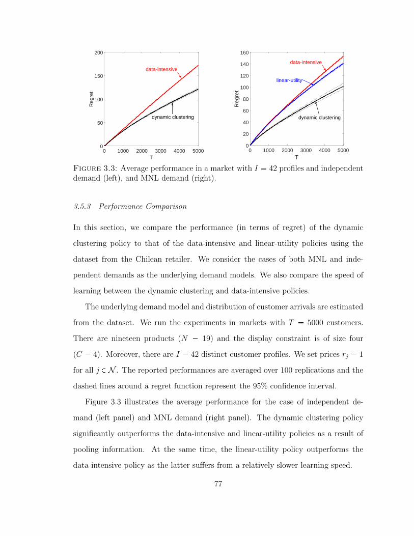
T0 1000 2000 3000 4000 5000

Reg

ret

0

50

100

150

200

data-intensive

dynamic clustering

T0 1000 2000 3000 4000 5000

Reg

ret

0

20

40

60

80

100

120

140

160

linear-utility

data-intensive

dynamic clustering

Figure 3.3: Average performance in a market with I 42 profiles and independentdemand (left), and MNL demand (right).

3.5.3 Performance Comparison

In this section, we compare the performance (in terms of regret) of the dynamic

clustering policy to that of the data-intensive and linear-utility policies using the

dataset from the Chilean retailer. We consider the cases of both MNL and inde-

pendent demands as the underlying demand models. We also compare the speed of

learning between the dynamic clustering and data-intensive policies.

The underlying demand model and distribution of customer arrivals are estimated

from the dataset. We run the experiments in markets with T 5000 customers.

There are nineteen products (N 19) and the display constraint is of size four

(C 4). Moreover, there are I 42 distinct customer profiles. We set prices rj 1

for all j P N . The reported performances are averaged over 100 replications and the

dashed lines around a regret function represent the 95% confidence interval.

Figure 3.3 illustrates the average performance for the case of independent de-

mand (left panel) and MNL demand (right panel). The dynamic clustering policy

significantly outperforms the data-intensive and linear-utility policies as a result of

pooling information. At the same time, the linear-utility policy outperforms the

data-intensive policy as the latter suffers from a relatively slower learning speed.

77

Figure 3.4 (left panel) illustrates the evolution of the root mean squared error

(RMSE) of estimated MNL parameters (i.e., exponentiated mean utilities) for the

dynamic clustering and data-intensive policies in the case of the MNL demand model.

This error is averaged over all products and profiles. As noted from the graph, the

RMSE associated with the dynamic clustering policy decreases significantly faster

than that of the data-intensive policy, implying a faster learning speed. The right

panel of Figure 3.4 shows the evolution of the average number of clusters that emerge

from the dynamic clustering policy over time (i.e., over customer arrivals). As can

be noted from the graph, early on in the selling season, when only a limited number

of transactions have been observed, the average number of clusters is small. That

is, the policy pools transaction information across a large number of customer pro-

files. As more transaction data is collected, the dynamic clustering policy refines the

composition of customer segments (clusters) and better personalizes the assortment

offerings using a larger number of clusters.

In sum, the dynamic clustering policy outperforms the data-intensive and linear-

utility policies in terms of regret (i.e., revenue collection) in the case study based on

the Chilean retailer’s dataset. We find that, under the MNL model, the dynamic

clustering policy results (on average) in 37.7% and 27.3% additional transactions

compared to the data-intensive and linear-utility policies, respectively. Moreover, the

dynamic clustering policy results in more than 65% additional transactions compared

to a randomized assortment policy (which was used by the retailer while collecting the

data). Furthermore, the dynamic clustering policy has a significantly faster learning

speed compared to the data-intensive policy. The proposed policy pools information

across most profiles early on in the selling season, but personalizes the assortment

offerings as more transaction data becomes available.

78

0 1000 2000 3000 4000 5000T

0

0.2

0.4

0.6

0.8

1

RM

SE

data-intensive

dynamic clustering

T×104

1 2 3 4 5

Ave

rage

Num

ber

of C

lust

ers

1

2

3

4

5

6

7

8

Figure 3.4: Speed of learning for different policies (left) and the evolution of theaverage number of clusters under the dynamic clustering policy (right) for MNLdemand and I 42.

3.5.4 Customer Attributes

In this section, we study the impact of a finer definition of customer attributes

on policy performance. Moreover, we compare the computation times of different

policies and illustrate the efficiency and scalability of the dynamic clustering policy.

In addition, we discuss an approach to further expedite the computation time of the

dynamic clustering policy. We finally discuss how one can incorporate management

knowledge about customer similarity into the dynamic clustering policy.

As discussed before, the retailer uses 42 different customer profiles, based on

their understanding of the Chilean retail market. For example, the attribute corre-

sponding to the customer’s location is based on the retailer’s knowledge about the

customer base in Chile (e.g., urban versus rural locations, etc.). The retailer also

groups customers according to their ages into three age groups r0, 29s, r30, 39s, and

r40, 99s, presumably based on an understanding of different purchasing patterns of

customers in each of these three groups. In order to study the impact of a finer

definition of customer attributes, we have extended the study beyond the 42 origi-

nal customer profiles used by the retailer. The raw dataset available to us contains

79

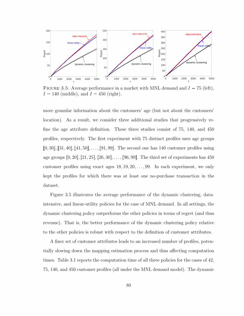
T0 1000 2000 3000 4000 5000

Reg

ret

0

50

100

150

200

data-intensive

linear-utility

dynamic clustering

T0 1000 2000 3000 4000 5000

Reg

ret

0

50

100

150

200

250

linear-utility

dynamic clustering

data-intensive

T0 1000 2000 3000 4000 5000

Reg

ret

0

50

100

150

200

250

300

350

400

linear-utility

dynamic clustering

data-intensive

Figure 3.5: Average performance in a market with MNL demand and I 75 (left),I 140 (middle), and I 450 (right).

more granular information about the customers’ age (but not about the customers’

location). As a result, we consider three additional studies that progressively re-

fine the age attribute definition. These three studies consist of 75, 140, and 450

profiles, respectively. The first experiment with 75 distinct profiles uses age groups

r0, 30s, r31, 40s, r41, 50s, . . . , r91, 99s. The second one has 140 customer profiles using

age groups r0, 20s, r21, 25s, r26, 30s, . . . , r96, 99s. The third set of experiments has 450

customer profiles using exact ages 18, 19, 20, . . . , 99. In each experiment, we only

kept the profiles for which there was at least one no-purchase transaction in the

dataset.

Figure 3.5 illustrates the average performance of the dynamic clustering, data-

intensive, and linear-utility policies for the case of MNL demand. In all settings, the

dynamic clustering policy outperforms the other policies in terms of regret (and thus

revenue). That is, the better performance of the dynamic clustering policy relative

to the other policies is robust with respect to the definition of customer attributes.

A finer set of customer attributes leads to an increased number of profiles, poten-

tially slowing down the mapping estimation process and thus affecting computation

times. Table 3.1 reports the computation time of all three policies for the cases of 42,

75, 140, and 450 customer profiles (all under the MNL demand model). The dynamic

80

clustering policy requires the estimation of the mapping (by running the MCMC). In

Table 3.1, we separate the running time of a customer arrival for which the mapping

is updated (noted as MCMC) and the running time of those arrivals for which there is

no mapping update (in which case the policy uses the prevailing mapping of profiles

to clusters). Similarly, the linear-utility model requires the estimation of attribute-

specific parameters through the maximum likelihood estimation (MLE). Table 3.1

reports the running time of a customer arrival for which the attribute-specific param-

eters are updated (noted as MLE) and the running time of those arrivals in which

there is no parameter update (and for which the linear-utility policy operates under

the prevailing estimates). The computation time of the MCMC and MLE increases

with the granularity of customer attributes (and therefore the number of customer

profiles).

The computation time of the dynamic clustering policy is reasonable and scales

well with the number of profiles. All experiments were run on a personal computer

– a retailer with more sophisticated computational resources would experience even

faster results. Note that, as expected, the data-intensive policy has the fastest com-

putation time (at the expense of a lower revenue performance), as this policy treats

each profile independently. The dynamic clustering policy can also handle a large

number of products without significantly affecting computation times. In the estima-

tion stage, the number of products impacts the calculation of the likelihood functions

and the updates of preference parameters, which are computed in closed-form as dis-

cussed in Section 3.4.3. For the assortment optimization stage, there are efficient

algorithms for the MNL model (for example, the algorithm in Rusmevichientong

et al. (2010) scales polynomially in the number of products). The optimization in

the case of independent demand is trivial.

We next discuss an approach to further improve the computation time of the

dynamic clustering policy, without significantly impacting its performance. This

81

Table 3.1: Average computation time (in seconds) of different policies for MNLdemand and T 5000.

Dynamic Clustering Linear-Utility Data-IntensiveNo mapping update MCMC No parameter update MLE Each customer arrival

I 42 0.00031 1.0818 0.00017 2.7827 0.00015I 75 0.00039 1.7121 0.00018 3.9762 0.00015I 140 0.00054 2.9850 0.00018 5.9750 0.00016I 450 0.00117 8.1729 0.00018 9.1619 0.00017

approach involves reducing the number of customer profiles for clustering purposes.

In particular, this version of the dynamic clustering policy considers customer profiles

within each specific location in isolation and therefore the policy runs the MCMC

for different locations in parallel. We refer to this version of the dynamic clustering

policy as “Location-DC.” Table 3.2 below reports the computation times of this

version of the dynamic clustering policy, together with that of the original policy

(which we refer to as “Original-DC”), for the setting with I 450 profiles and

MNL demand. As can be noted from the table, the “Location-DC” version of the

policy brings significant savings in terms of computation time. While this version is

slightly outperformed by the original dynamic clustering policy in terms of regret, it

still performs significantly better than the data-intensive and linear-utility policies.

Table 3.2: Average computation time (in seconds) of the original and a location-based version of the dynamic clustering policy for MNL demand with I 450 andT 5000. No mapping update MCMC

Original-DC 0.00117 8.1729Location-DC 0.00048 1.5575

We finally discuss how one can incorporate management knowledge about cus-

tomer similarity into the dynamic clustering policy. Suppose that existing manage-

ment insight indicates that “neighboring” profiles (e.g., two profiles with the same

gender and location and very close in age) are likely to have “similar” preferences for

products. The dynamic clustering algorithm can accommodate management knowl-

edge about customers by restricting attention to mappings that only group “neigh-

boring” profiles. (This can be implemented in the MCMC sampling procedure: while

82

updating the cluster label ci of a customer with profile given by a vector xi, the can-

didate cluster label is drawn only from clusters that currently include profiles that are

“similar” to xi – the notion of similarity can be formally defined based on attributes.)

An alternative approach consists of merging upfront profiles that are known to have

similar preferences for products. For example, it may be that, based on an under-

standing of the customer base, management is confident that customers from two

particular ZIP codes or locations have similar tastes for products. Unlike the previ-

ous approach, these customer profiles with similar preferences may not have similar

attributes. One can use this additional information to speed up the learning process

by grouping such profiles together before running the dynamic clustering algorithm.

In sum, we find that the better performance of the dynamic clustering policy

relative to the other policies is robust with respect to the definition of customer

attributes. At the same time, a finer definition of customer attributes (i.e., a larger

number of customer profiles) increases the computation time. However, we show that

the computation time of the dynamic clustering policy is still reasonable and scales

well with the number of profiles. One can further expedite the computation time of

the policy by reducing the number of customer profiles for clustering purposes.

3.5.5 Comparison to Linear-Utility Model

In this section, we compare the dynamic clustering policy to the linear-utility ap-

proach in more detail. We first discuss the advantages of each approach and then

introduce a set of experiments to compare the performance of the two policies.

In addition to better performance of the dynamic clustering policy over the linear-

utility model, the dynamic clustering policy has several other advantages. Retailers

are generally interested in identifying customer segments (i.e., clusters of customers

with similar preferences). These segments are part of the output of the dynamic

clustering policy and can be interpreted based on customers’ attributes – see Figure

83

3.6 below for a representative example based on the dataset from the Chilean retailer.

Figure 3.7 also illustrates the optimal assortments for different clusters in an example

in which the profiles only differ by their geographical location in Chile. Moreover,

the mean utilities may not be linear in customer attributes. The dynamic clustering

policy makes no assumption about the structure of the mean utilities with respect

to customer attributes. In particular, the transaction dataset from the Chilean re-

tailer exhibits a non-linear dependence between mean utilities and attributes. In

such cases, the linearity assumption could result in inaccurate estimates which, in

turn, could hurt the retailer’s revenue. Also, the dynamic clustering policy takes a

Bayesian approach and is designed to expedite the learning process, especially in the

short-term when the amount of transaction data is limited. Overall, the dynamic

clustering policy leads to 27.3% more transactions (on average) than the linear-utility

policy in the experiments based on the dataset under the MNL demand model. The

linear-utility approach, however, uses maximum-likelihood estimation and thus is

better suited for (offline) settings with large amounts of transaction data. As such,

the linear-utility approach can identify whether an attribute is statistically signifi-

cant (relevant) through the estimates of the attribute-specific parameters. One can

make similar observations based on the output of the dynamic clustering policy. For

example, as noted in Figure 3.6, customers in Santiago West tend to have different

preferences for products than customers from Santiago East.

Because the linear-utility approach may be better suited for an offline setting,

we designed an additional set of experiments which mimic an offline setting. More

specifically, because the estimation approach (and underlying model assumption) is

different under the dynamic clustering and linear-utility policies, we further compare

the performance of these policies in a setting in which the performance is mainly

affected by the quality of estimation which, in turn, impacts the assortment deci-

sions made by different policies. To that end, we consider separation-based versions

84

North

Far South

Far North

Santiago West

Center

South

Cluster 2

Cluster 1

Cluster 3

Cluster 4

Far North

Far South

Santiago West

Santiago East

Center

South

Cluster 1

Cluster 2

Cluster 3

North

Santiago EastCluster 5

Cluster 6

Cluster 4

Cluster 5

Far North

Far South

Santiago West

Santiago East

Center

South

Cluster 1

Cluster 2

Cluster 3

North

Cluster 5

Cluster 6

Cluster 4

Figure 3.6: Illustration of clusters (under the most likely mapping) for women fromage groups r0, 29s (left), r30, 39s (middle), and r40, 99s (right) based on customers’location in Chile.

Far North

Far South

Santiago West

Santiago East

Center

South

Cluster 1

Cluster 2

Cluster 3

North

Cluster 4

Cluster 5

Figure 3.7: Illustration of optimal assortments for women from age group r30, 39s.

of these policies, which separate exploration from exploitation. In the separation-

based experiments, we randomly generate a sample of transaction data with random

85

assortment offerings and random customer arrivals based on the estimated MNL pa-

rameters and arrival distribution of profiles from the dataset. All policies use the

same sample to estimate the MNL parameters (exploration stage). Each policy then

finds the optimal assortment for each customer profile. We then generate another

random sample of customer arrivals with the same size as that used in the exploration

phase (according to the estimated arrival distribution) over which each policy offers

its personalized optimal assortment to each arriving customer (exploitation stage).

We consider the cumulative regret and revenue of all policies only for the exploitation

phase as all policies use the same sample (and thus incur the same regret) in the

exploration phase. As a result, any difference in performance is due to the quality

of estimation. We consider two scenarios in terms of the underlying demand model.

The first scenario is based on the original transaction dataset, which exhibits

a non-linear dependence of mean utilities on customer attributes. We experiment

with different sample sizes T . The dynamic clustering policy outperforms both the

data-intensive and linear-utility policies in all instances. Table 3.3 below reports the

percentage improvement of the dynamic clustering policy over the other policies, both

in terms of regret and revenue (i.e., expected number of transactions). The revenue

improvements can be as high as 50% and 25.4% compared to the data-intensive and

linear-utility policies, respectively. Moreover, the improvements are generally higher

for smaller samples sizes, as the dynamic clustering policy performs particularly well

in settings with limited transaction data by pooling information. Table 3.4 reports

the average estimation times (i.e., computation time of MCMC and MLE for the

dynamic clustering and linear-utility policies, respectively). As expected, the data-

intensive policy has the lowest computation time as the estimation can be done

independently for each customer profile. The linear-utility model is faster than the

dynamic clustering policy for smaller sample sizes. However, its computation time

increases significantly for larger sample sizes, suggesting that the linear-utility policy

86

may be better suited for an offline setting.

Table 3.3: Average percentage improvement of dynamic clustering policy over data-intensive and linear-utility policies in separation-based experiments using the originaldataset.

Regret RevenueData-Intensive Linear-Utility Data-Intensive Linear-Utility

T 500 34.2% 24.6% 47.8% 25.4%T 1000 42.6% 28.4% 50.0% 21.6%T 5000 39.0% 26.6% 20.7% 10.7%T 10000 24.3% 12.9% 8.9% 3.9%T 20000 6.7% 3.6% 1.5% 0.8%

Table 3.4: Average estimation time (in seconds) in separation-based experimentsbased on original dataset.

T 500 T 1000 T 5000 T 10000 T 20000Dynamic Clustering 1.214 1.301 2.307 3.861 7.010

Data-Intensive 0.003 0.006 0.025 0.048 0.096Linear-Utility 0.508 0.922 5.872 13.877 31.168

While the original dataset does not exhibit a linear dependence on customer at-

tributes, we generate a second set of (synthetic) experiments in which the underlying

demand model is linear as in (3.7). To that end, we estimate βj in model (3.7) for

each product j from the dataset and use such estimates to randomly generate syn-

thetic (linear) transaction data for simulation. We find that the dynamic clustering

policy outperforms the linear-utility approach in all instances except for that with

the largest transaction sample (i.e., T 20000) – please refer to Table B.1 in Ap-

pendix B.2 for a summary of the results of this numerical study. This suggests that

the benefit of pooling information achieved by clustering can lead to better perfor-

mance even when the underlying demand model is, in fact, linear. Such benefits are

more pronounced in the short-term, i.e., for small and moderate sample sizes.

To conclude, the dynamic clustering policy outperforms the linear-utility ap-

proach in the case study based on the Chilean retailer’s dataset. Each approach has

its advantages and may be deemed more appropriate depending on the specific set-

87

ting. For example, the retailer that provided the dataset is interested in identifying

customer segments (i.e., clusters of customers with similar preferences). These seg-

ments are part of the output of the dynamic clustering policy and can be interpreted

based on customers’ attributes (as in the examples in Figures 3.6 and 3.7).

3.6 Value of Pooling Information

In this section, we provide analytical support for the insights derived in the case

study in Section 3.5. More specifically, this section explores the impact of pooling

information about customers’ preferences on the retailer’s revenue by considering a

stylized version of the dynamic assortment personalization problem. To this end, we

focus on three policies that differ in the extent by which they aggregate information

across customers. The data-intensive policy, described in Section 3.5.2, treats cus-

tomer profiles independently to estimate preferences and make assortment decisions.

We further introduce a semi-oracle policy that knows upfront the underlying map-

ping of profiles to clusters but not the customer preferences for each cluster. The

semi-oracle policy reflects the key element of the dynamic clustering policy – in that

it pools transaction information across customers with similar preferences – but it

bypasses the estimation of the mapping of profiles to clusters by assuming that it

is known to the retailer. Working with the dynamic clustering policy analytically is

not possible, as it requires a Bayesian update of the mapping that cannot be done

in closed-form. In the other extreme, we consider a pooling policy that aggregates

transaction data across all customer profiles (regardless of whether the customers

have similar preferences or not). We show that the semi-oracle outperforms the

data-intensive policy. Moreover, we analytically characterize settings in which the

pooling policy outperforms the data-intensive policy.

All policies we consider in this section – the data-intensive policy (πd-int), the

semi-oracle policy (πs-orc), and the pooling policy (πpool) – follow the same bandit

88

algorithm to determine what assortment to offer each arriving customer. The policies,

however, differ in how they use the available information to estimate the customers’

preferences and make assortment decisions. For ease of analysis, we focus on the

independent demand model in this section.8 We also assume, for tractability, that

C 1 and rj 1 for all products j P N .

LetRπd-int , Rπs-orc , andRπpool denote the regrets associated with the data-intensive,

semi-oracle, and pooling policies, respectively. To simplify notation, we denote them

as Rd-int, Rs-orc, and Rpool hereafter. We further define the gap functions

G1 : Rd-int Rs-orc and G2 : Rd-int Rpool.

Our goal is to determine conditions under which these gaps are non-negative. Because

characterizing the regret functions in closed-form is not possible, we use upper bounds

on the regret for the semi-oracle and pooling polices, denoted by Us-orc and Upool,

respectively, and a lower bound on the regret for the data-intensive policy, denoted

by Ld-int. Therefore, Ld-int Us-orc provides a lower bound for the gap function G1

and Ld-int Upool provides a lower bound for the gap function G2. Hence, we focus

on characterizing settings in which these lower bounds are non-negative, which in

turn implies that G1, G2 ¥ 0.9 Lai and Robbins (1985a) prove an asymptotic lower

bound (for large T ) on the achievable performance of any consistent policy in the

classic bandit setting (i.e., with a homogeneous population of customers).10 Roughly

speaking, the long-run number of mistakes (associated with pulling suboptimal arms)

under any consistent policy is smaller than T a for large T and every a ¡ 0. In

particular, it is smaller than a linear function of T , which corresponds to making

8 One can obtain similar results for the MNL demand model as well.

9 While the lower bounds are not always tight, the goal is to show the non-negativity of the gapfunctions. As a result, working with the bounds enables the analysis and leads to the desired results.

10 An admissible policy π is consistent if, for any distribution of preferences F (that satisfies certain

regularity conditions), RπpT qTa Ñ 0, as T Ñ 8, for every a ¡ 0. That is, if RπpT q opT aq. See Lai

and Robbins (1985a).

89

mistakes for every customer. Let P 1 P denote the set of consistent admissible

policies. We restrict attention to consistent policies π P P 1 and use Lai and Robbins’

lower bound to derive Ld-int. More specifically, we derive a lower bound on the regret

associated with each profile and define Ld-int as the sum of these lower bounds.

The upper bounds on the regrets for the semi-oracle and pooling policies depend

on the specific bandit algorithm used for selecting the product to offer each arriv-

ing customer. We focus here on the celebrated upper confidence bound (UCB1)

policy of Auer et al. (2002). After an initialization phase during which each prod-

uct is offered once, UCB1 offers customer t a product j with the highest index

µja

2 lnpt 1qkjpt 1q, where µj is the sample mean of the number of purchases

for product j, and kjpt1q is the number of times that product j has been offered up

to (and including) time t 1. The UCB1 policy is easy to implement and its regret

admits a finite-time upper bound which is simple to use. We extend the results of

Sections 3.6.1 and 3.6.2 for Thompson Sampling in Appendix B.2.

3.6.1 Semi-Oracle

In this section, we compare the performance of the data-intensive policy to that of

the semi-oracle policy. As expected, the semi-oracle outperforms the data-intensive

policy in terms of regret (i.e., revenue). This result emphasizes the benefit of es-

timating the mapping of profiles to clusters (as in the dynamic clustering policy)

as it helps expedite the learning process by pooling transaction information across

customer profiles within a cluster. (We provide a formal statement and proof of the

result in Theorem 33 in Appendix B.1.)

We next show that there are diminishing marginal returns to pooling information

from an increasing number of customer profiles. To that end, consider a general

market with K clusters where 1 ¤ K I. We assume, without loss of generality, that

K I, since if K I, then both the semi-oracle and data-intensive policies incur

90

the same regret and therefore G1 0. Let Ik denote the set of profiles belonging

to cluster k and Ik : |Ik|. Also, let I 1 : pI1, . . . , IKq. This vector summarizes

the mapping of profiles to clusters. We assume, without loss of generality, that

product 1 has the highest purchase probability for each profile, i.e., µij µi1 for

j 2, . . . , N and all i P I. Computing the lower bound Ld-int Us-orc for the gap

function G1 requires an additional approximation as the setting studied in Lai and

Robbins (1985a) considers a homogeneous population of customers. This additional

approximation involves a first-order Taylor expansion and, as such, the resulting

approximate lower bound is very close to Ld-intUs-orc. We denote by G1lpT, I 1q the

approximation to the lower bound for the gap function G1. This approximate lower

bound depends on the total number of customer arrivals T and on the vector I 1

which encodes the mapping of profiles to clusters. We provide a detailed derivation

of G1lpT, I 1q in Appendix B.1.

Theorem 13. Consider the case of uniform arrivals within each cluster, i.e., pi

PkIk for all i P Ik where Pk :°iPIk pi is constant. We then have that G1lpT, I 1q

is increasing in Ik for T ¡ eIkPk pe is the Euler’s numberq and concave in Ik for

T ¥ 1.

Theorem 13 shows the first- and second-order effects of the number of customer

profiles Ik on the approximate lower bound. We find that, for sufficiently large

T , G1lpT, I 1q is increasing in the number of profiles Ik. That is, the benefit of

pooling information increases with the number of profiles within any cluster k, as it

becomes increasingly more time-consuming for the data-intensive policy to learn the

preferences of each customer profile when Ik increases. In addition, the result shows

that G1lpT, I 1q is concave in Ik. That is, there are diminishing marginal returns

to pooling information from an increasing number of customer profiles within any

cluster.

91

We also explore whether the result in Theorem 13 applies to the dynamic cluster-

ing policy and MNL demand model by considering an example based on the dataset

from the Chilean retailer. Specifically, we estimate the MNL parameters for the cus-

tomer profile (female, r40, 99s, Center) from the dataset and assume that a cluster’s

demand follows such MNL model. We then increase the number of profiles in that

cluster and evaluate the gap between the regrets of the data-intensive and dynamic

clustering policies in a market with T 5000 customers. Figure 3.8 shows the result

of this experiment, where Rd-int and Rdc denote the regrets of data-intensive and

dynamic clustering policies, respectively. As noted in the graph, and consistent with

Theorem 13, the (actual) gap between the regrets of the two policies is increasing

and concave in the number of customer profiles within the cluster.

I2 4 6 8 10

Rd-

int-R

dc

10

20

30

40

50

60

70

Figure 3.8: Gap between the regrets of data-intensive and dynamic clusteringpolicies as a function of number of profiles.

3.6.2 Pooling in the Short-Term

In this section, we consider a setting with heterogeneous customers and a pooling pol-

icy that aggregates information across all customer profiles. As one would expect,

pooling information across all customer profiles is not necessarily beneficial for the

retailer in a heterogeneous market as it could lead to erroneous estimates. However,

92

we show that, under some conditions, the pooling policy tends to outperform the

data-intensive policy in the short-term even if customer preferences are heteroge-

neous. This, in turn, allows us to examine the key drivers of efficiency gains derived

by pooling information.

Consider a market with K ¥ 2 clusters. Without loss of generality, we assume

that K N , where N is the number of products. We also assume that cluster k’s

customers have the highest purchase probability for product k, for k 1, . . . , K.

Furthermore, we assume that µkk µkj ∆ for some ∆ ¡ 0 and for all k 1, . . . , K

and j k, where, to simplify notation, µkj denotes the purchase probability of

product j for all profiles in cluster k. Let P : pP1, P2, . . . , PKq where Pk °iPIk pi is

the proportion of profiles belonging to cluster k. We also define P 1 : pP2, . . . , PK1q.

We assume, without loss of generality, that Pk P1 ¤ 1 for all k 2, . . . , K. Note

that P1 is a measure of heterogeneity in this setting and a smaller P1 leads to a more

heterogeneous customer population. In the extreme, P1 1 reduces this setting to

one with a homogeneous market.

As in Section 3.6.1, we consider an approximate lower bound on the regret of

the data-intensive policy, based on Lai and Robbins (1985a). Existing upper bounds

in the bandit literature (including that of the UCB1 policy) assume a homogeneous

market. This introduces additional complexity in the computation of the upper

bound on the regret of the pooling policy. This upper bound is derived in Appendix

B.1. Let G2lpt, I, P q be the approximation of the lower bound Ld-int Upool to the

gap function G2 at any time period t. We provide a detailed derivation of G2lpt, I, P q

in Appendix B.1. The next result provides conditions under which the pooling pol-

icy outperforms the data-intensive policy (subject to the approximations), that is,

G2lpt, I, P q ¥ 0.

93

Theorem 14. Consider the case of uniform arrivals, i.e., pi 1I for all i P I.

There exist thresholds IlpP q and P1pI, P1q such that if I ¥ IlpP q and P1pI, P

1q

P1 ¤ 1, then

G2lpt, I, P q ¥ 0 for tlpI, P q ¤ t ¤ tupI, P q,

with 1 tlpI, P q ¤ tupI, P q ¤ 8. Moreover, IlpP q and P1pI, P1q are non-increasing

in P1 and I, respectively.

The result in Theorem 14 shows that, under some conditions, the pooling policy

tends to outperform the data-intensive policy for a range of customer arrivals, even if

the retailer learns the customers’ preferences inaccurately in a heterogeneous market

under the pooling policy. This is the result of faster learning under the pooling

policy achieved by aggregating information across all customer profiles. In particular,

Theorem 14 illustrates the benefit of pooling information in the short-term, when

transaction data is limited. Moreover, Theorem 14 implies that three key factors

favor the performance of the pooling policy over the data-intensive policy:

• Heterogeneity (P1): If the population is not too heterogeneous (i.e., if P1 ¡

P1pI, P1q), then the pooling policy tends to outperform the data-intensive pol-

icy for a range of customer arrivals. This is because, under such condition, the

benefit associated with faster learning by aggregating information outweighs

the cost associated with the errors the pooling policy makes by not differenti-

ating between clusters (and therefore offering suboptimal assortments). More-

over, the threshold P1pI, P1q decreases as the number of profiles increases.

• Number of profiles (I): An increase in the number of profiles impacts negatively

on the performance of the data-intensive policy. As I increases, the average

number of customer arrivals per profile decreases and thus it takes longer for

the data-intensive policy to learn the preferences for each profile. On the other

94

hand, the pooling policy aggregates information across all customers and thus

its performance does not degrade as long as P1 ¡ P1pI, P1q. As the population

becomes more homogeneous in terms of preferences (i.e., as P1 increases), the

pooling policy tends to outperform the data-intensive policy for an even smaller

number of customer profiles.

• Number of Customers (t): Although a relatively more homogeneous market

and a large number of profiles can favor the performance of the pooling policy,

the key factor is the amount of transaction information available to the retailer.

When the number of customer arrivals is still relatively small, the data-intensive

policy does not have enough sample points to accurately learn the preference

of each customer profile. On the other hand, the pooling policy aggregates

information and therefore tends to outperform the data-intensive policy as

long as the population is not too heterogeneous with respect to their product

preferences. As more customers arrive, the performance of the data-intensive

policy prevails. In particular, G2lpt, I, P q Ñ 8 (and G2pt, I, P q Ñ 8) as

tÑ 8 if P1 1.

The result in Theorem 14 is consistent with the observations about the dynamic

clustering policy illustrated in the right panel of Figure 3.4. Early on in the selling

season, when only a limited number of transactions have been observed, the average

number of clusters that emerge from the dynamic clustering policy is small. This

echoes the preceding discussion – when limited information is available, the retailer

might be better off pooling all available data (even if they correspond to profiles

with different preferences) to speed up the learning process. The number of clusters

then increases as more data becomes available (as can be noted in the right panel of

Figure 3.4) and the retailer is able to personalize the assortment offerings by better

matching customer preferences.

95

3.7 Conclusion

This paper considers a retailer endowed with multiple products that dynamically

personalizes the assortment offerings over a finite selling season. Customers are

assigned to different profiles based on their observable personal attributes. Their

preferences are unknown to the retailer and must be learned over time. The pri-

mary goal of the paper is to explore the efficient use of data in retail operations

and its benefits (in terms of revenue) for assortment personalization. To that end,

we propose the dynamic clustering policy as a prescriptive approach for assortment

personalization in an online setting. We take advantage of existing tools from the

literature and introduce a policy that adaptively combines estimation (by estimat-

ing customer preferences through dynamic clustering) and optimization (by making

dynamic personalized assortment decisions using a bandit policy) in an online set-

ting. The dynamic clustering policy adaptively adjusts the composition of customer

segments (i.e., mapping of profiles to clusters) based on the observed customers’ pur-

chasing decisions. The policy exploits the similarity in preferences of customers in the

same cluster by aggregating their transaction information and expediting the learn-

ing process. Using the estimated mapping and preferences, the policy uses existing

bandit algorithms to make assortment decisions.

To illustrate the practical value of the dynamic clustering policy in a realistic set-

ting, we apply the policy to a dataset from a large Chilean retailer. We compare the

performance of the dynamic clustering policy with two alternatives: a data-intensive

policy that treats each customer profile independently and a linear-utility policy that

estimates product mean utilities as linear functions of customer attributes. The case

study suggests that the dynamic clustering policy can significantly increase the av-

erage number of transactions relative to the other policies. We also demonstrate the

scalability and efficiency of the dynamic clustering policy in terms of computation

96

time.

We then study a simplified version of the problem in which the retailer offers a

single product to each arriving customer. We show that a semi-oracle policy that

knows upfront the mapping of profiles to clusters (but not the customers’ prefer-

ences) outperforms the data-intensive policy, indicating that pooling information is

beneficial for the retailer. We also demonstrate that there are decreasing marginal

returns to pooling information as the number of customer profiles increases. Finally,

we characterize conditions under which a policy that pools information across all

customer profiles outperforms the data-intensive policy even when customer prefer-

ences are heterogeneous. This result emphasizes the benefit of pooling information

in the short-term, when there is insufficient data to accurately estimate preferences

for each customer profile.

In this work, we have made some simplifying assumptions for tractability. Fu-

ture work can take into consideration the presence of inventory constraints in the

model. Moreover, we have assumed that prices are constant throughout the sell-

ing season. Incorporating pricing decisions is another direction for future research.

Because the proposed approach relies on MCMC for estimation, the computational

cost is a potential concern for implementing the policy in a high-dimensional set-

ting in real-time; nonetheless, the paper discusses several approaches to expedite the

computation. Furthermore, the proposed approach does not assume any particular

relation between the products’ mean utilities and customer attributes. In a high-

dimensional setting, imposing further structure on the utility model (e.g., similar to

the linear-utility approach) is a potential alternative to expedite the estimation.

97

4

Uncertainty in Choice: The Role of Return Policies

4.1 Introduction

Merchandise returns account for a considerable portion of annual retail sales. Ac-

cording to the National Retail Federation (Anonymous, 2017), total merchandise

returns in 2017 reached $351 billion for US retailers. This amount is equivalent to

10% of the total US retail sales in 2017. The size of returns is overwhelming as

it is close to the estimated 2017 federal budget deficit of $400 billion. Returns are

costly for the retailers as they result in reverse logistic costs for handling the returns.

Product returns cost manufacturer and retailers more than $100 billion per year, or

an average loss per company of about 3.8% in profit (Petersen and Kumar, 2010).

According to AlixPartners, items returned to the store cost a retailer roughly $3 to

process and are available for resale within a day. Items shipped back to a distribution

center or third-party logistics provider cost $6 or more to process and take at least

four days before they are available for resale (Phillips, 2017).

Despite its handling costs, retailers recognize the value of offering a return option

to customers as it allows them to return unwanted products. This is especially

98

important for online shoppers as they are unable to fully evaluate the product at

the time of purchase (e.g., the exact fit of a piece of clothing). As a result, many

customers rely on product returns as part of their shopping process.

To reduce the cost and frequency of product returns, some companies create

product-return disincentives such as limited time frames for returns (e.g., within 30

days after purchase) or charging a return fee (e.g., a restocking fee). However, several

recent studies have shown the potential positive impacts of returns. For example,

Petersen and Kumar (2010) find that when a company has a lenient return policy,

customers are more willing to make other purchases. Thus, the question of how

lenient the retailers should be in offering their return policies still remains somewhat

unanswered: on one hand, the retailer incurs reverse logistic costs to handle returned

products; on the other hand, however, customers value the option of return and this,

in turn, could have positive impacts on retailer’s (future) sales.

In this paper, we study the interplay between a retailer’s return and pricing poli-

cies and customers’ purchasing decisions. More specifically, we model the customers’

purchasing and returns decisions using a discrete choice model and study how such

decisions are impacted by the retailer’s pricing and return policies. We study three

main research questions in this work: piq how the pricing decision of the retailer is

impacted by product returns; piiq what factors make the return option favorable for

the retailer (as opposed to not offering the return policy); piiiq what is the impact

of accounting for product returns on demand estimation.

We study the seller’s revenue maximization problem in the cases with and without

product returns. In the returns case, we consider a policy in which the seller fully

reimburses the customer for a returned product. We then model the customers’

purchasing and returns decisions using a discrete choice model. More specifically,

in the case without product returns, we model the customers’ purchasing decisions

as a Multinomial Logit (MNL) model. In the case with product returns, on the

99

other hand, we use a Nested MNL (N-MNL) to model customer’s purchasing and

returns decisions. In such case, customer’s choice can be viewed as a sequential

(two-stage) process in which the customer first decides between purchasing a product

from the offered assortment or choosing the outside option. Conditional on a product

purchase, the customer then decides whether to keep or return the purchased product.

We first focus on the single-product case and characterize the seller’s optimal price

in the cases with and without product returns. The results show that offering the

return option results in different (but not necessarily higher) optimal prices compared

to the case with no returns. Moreover, we find that offering the return option is not

always favorable for the retailer. In addition, we characterize conditions under which

offering the return option to customers increases the retailer’s revenue.

We also numerically study the impact of accounting for product returns on de-

mand estimation. We experiment with a dataset from a large Chilean retailer (this

dataset was used in the second essay in this dissertation). The preliminary numerical

results suggest that our N-MNL model, which accounts for product returns, increases

demand estimation accuracy compared to models that do not consider product re-

turns in their estimation.

The remainder of this paper is organized as follows. Section 4.2 reviews the rel-

evant literature. Section 4.3 describes the customer’s choice model and Section 4.4

models the seller’s revenue maximization problem. Section 4.5 discusses the prelimi-

nary analytical results. Section 4.6 numerically studies the impact of accounting for

product returns on demand estimation. Section 4.7 provides concluding remarks and

future research directions. All proofs are relegated to Appendix C.1.


Product returns and their impact on customers and retailers have been extensively

studied in the literature from both theoretical and empirical perspectives. We first

100

briefly discuss the analytical work and then review the empirical research.

There is an extensive body of literature on return policies. The classic work of

Pasternack (1985) studies the optimal pricing and return policies of a manufacturer

in a newsvendor setting. Davis et al. (1995) develop a simple model to characterize

conditions under which money-back guarantees are optimal. Che (1996) shows that

the seller adopts the (full-refund) return policy (as opposed to a no-return policy)

when consumers are highly risk averse or retail costs are high. Moorthy and Srini-

vasan (1995) find that full refunds may signal high quality. Several other papers focus

on preventing inappropriate returns when customers have no intention of keeping the

purchased products. For example, Hess et al. (1996) show that in the context of mail-

order catalogs, inappropriate returns can be controlled by imposing nonrefundable

charges that increase with the value of the merchandise ordered. Davis et al. (1998)

develop an analytical model to identify potential causes of variation among retailers’

return policies and support their insights empirically.

More recently, Shulman et al. (2009) develop an analytical model to characterize

the seller’s optimal pricing and restocking fee policy while taking into account the

customers’ strategic behavior. They also identify conditions under which it is (or

not) optimal to provide product fit information to customers. Su (2009) studies the

optimal price, quantity, and refund amount decisions of a seller in a newsvendor

setting and investigates the impact of different return policies on supply chain per-

formance. Altug and Aydinliyim (2016) study the impact of consumer’s strategic

purchase deferrals on an online retailer’s return policy. Nageswaran et al. (2017)

study the pricing and return policy decisions of an omnichannel retailer.

In contrast to the papers discussed above, we model the customer’s purchasing

and returns decisions using a discrete choice model. Closest to ours in terms of

the model is the work by Alptekinoglu and Grasas (2014) which uses the N-MNL

framework to model the customer’s choice. The authors study how the optimal

101

assortment decision of a retailer is impacted by its return policy. We, however,

focus on the pricing decision of the retailer. Moreover, the return policy is a decision

variable in our model while in Alptekinoglu and Grasas (2014) the return policy (and

prices) are exogenous. Wang and Sahin (2017) study the impact of consumer search

cost on assortment and pricing decisions of a retailer. They model the consumer

choice as a two-stage “consider-then-choose” process by incorporating the search

cost into the consumer choice model. In a similar setting, Wagner and Martınez-de

Albeniz (2017) study pricing and assortment decisions of a retailer when customers

learn about products’ value in a sequential product exchange process.

Product returns have also been widely studied using empirical studies. We pro-

vide a few examples here. Petersen and Kumar (2009) empirically determine the

factors that help explain product return behavior and the consequences of prod-

uct returns on future customer and firm behavior. The paper shows that increases

in product return increase future customer purchases up to a threshold. Anderson

et al. (2009) develop a structural model to measure the value of the return option to

consumers. Petersen and Kumar (2015) conduct a large-scale field experiment and

show that the firm can increase its profit by accounting for the customer’s perceived

risk related to product returns in addition to managing product return costs. In

our paper, we aim at understanding the impact of accounting for product returns

on demand estimation accuracy using a discrete choice model. To the best of our

knowledge, this issue has not been studied in the existing literature.

4.3 Customer’s Choice Model

In this section, we model the customer’s choice given the seller’s return policy. Sup-

pose that a customer arrives at the store and faces a category of substitutable prod-

ucts. The full assortment consists of n products, but the seller offers a subset or

assortment S. We model the customer’s purchasing decision using a discrete choice

102

model. Because offering the return option to the customer could impact the cus-

tomer’s purchasing decision, we consider the following two scenarios.

4.3.1 Non-Returnable Products

In this case, the products are non-returnable, and thus a purchase means a final sale.

We model customer’s purchasing decision using a Multinomial Logit (MNL) model.

More specifically, let product 0 denote the outside option (e.g., the no-purchase

option or purchasing the product from a competing retailer). The utility of choosing

product i P S Y t0u is given by a linear-in-parameter function of the form1

UNRi : wi µ1εi, where wi : βi pi, (4.1)

and where βi and pi denote the attractiveness (i.e., nominal mean utility) and price

of product i, respectively. The noise terms εi are unobservable by the seller and are

i.i.d. random variables following a standard Gumbel distribution. Moreover, µ1 ¡ 0

is the degree of heterogeneity between products2. Without loss of generality, we set

the mean utility of the outside option w0 0.

The customer purchases the product (including the outside option) with the high-

est utility UNRi . According to the MNL model, the purchase probability of product

i P S Y t0u is given by

PNRi :exppwiµ1q

1°hPS exppwhµ1q

.

(Note that PNRi depends on the assortment S, but we drop such dependence to

simplify the notation.)

1 The superscript NR in UNRi indicates the case with no product returns.

2 Note that having the noise term µ1εi in (4.1) is equivalent to having a noise term that follows aGumbel distribution with location 0 and scale µ1.

103

4.3.2 Returnable Products

In this case, we model the customer’s purchasing and returns decisions using the

Nested Multinomial Logit (N-MNL) framework in order to capture the impact of a

return option on the customer’s decision. In the N-MNL model, customer’s choice

can be viewed as a sequential (two-stage) process in which the customer first decides

between purchasing a product from the offered assortment or choosing the outside

option. Conditional on a product purchase, the customer then decides whether to

keep or return the purchased product. We discuss the model in further detail in what

follows, starting from the second stage.

Second Stage. Suppose that the customer has purchased product i P S in the

first stage. In the second stage, the customer revises her (perceived) utility for the

product after trying it out and evaluating other factors which were bypassed at the

time of purchase (e.g., similarity with other comparable items that she already has,

change of mind, others’ opinions, etc.). At this point, the customer decides whether

to keep or return the purchased product. (Note that if the customer chooses the

outside option in the first stage, the second stage is no longer relevant.) The utility

that the customer obtains from keeping or returning the product is given by

Ukeepi : wi µ2 ε

keepi , U return

i : c µ2 εreturni ,

where wi is the mean utility of product i minus its price and c ¡ 0 is the hassle

cost that the customer incurs in case she decides to return the product (e.g., the

additional trip to the store). Moreover, εkeepi and εreturni denote the customer’s post-

purchase uncertainty which are i.i.d. random variables following a standard Gumbel

distribution, and µ2 ¡ 0 is the degree of heterogeneity between the two options (i.e.,

a measure of post-purchase heterogeneity). Note that for simplicity, we assume that

in case of product returns, the seller fully reimburses the customer. This represents

104

a lenient return policy which seems to be common practice, at least for fashion

products (one can modify the model to represent the case in which the seller only

partially reimburses the customer).

Under the N-MNL model, the conditional probability of returning the product

i P S given that it was purchased in the first stage follows an MNL model and is

given by:

Preturni :exp

cµ2

exp

cµ2

exp

wiµ2

.First Stage. In the first stage, the customer decides between purchasing a product

from the offered assortment or choosing the outside option. At this point, the cus-

tomer does not know for certain if she would keep or return the product in the second

stage (i.e., she cannot observe the realization of the post-purchase uncertainties εkeepi

and εreturni ) if she decides to purchase the product in the first stage. Therefore, the

customer chooses an option with the highest utility while taking into account the un-

certainty in the second stage. More specifically, the utility that the customer obtains

from choosing product i P S Y t0u is given by3

URi : Ai µ1εi, (4.2)

where Ai denotes the expected utility of purchasing product i P S (i.e., after re-

evaluating the product and making the final return/keep decision in the second

stage). More specifically, we have thatAi : E

max!wi µ2 ε

keepi ,c µ2 ε

returni

)for i P S where E denotes the expectation. It can be shown that (see, e.g., Anderson

and De Palma (1992)) Ai is:

Ai µ2 ln

exp

c

µ2

exp

wiµ2

, for i P S, (4.3)

3 The superscript R in URi indicates the case with product returns.

105

up to an additive constant, and we set A0 kpcq ¤ 0 for the outside option (i.e.,

product 0), where kpcq is the expected utility of the outside option (in the case

of returnable products) which is an increasing function of the hassle cost c. (We

discuss this function in more detail in what follows.) Moreover, εi in (4.2) denote

the customer’s pre-purchase uncertainty which are i.i.d. random variables following a

standard Gumbel distribution, and µ1 ¡ 0 is a measure of pre-purchase heterogeneity

– this is the same constant as that in (4.1). (We need the technical condition of

µ1 ¥ µ2 for the validity of the N-MNL model (Anderson and De Palma 1992). This

assumption has been used in the literature and is reasonable – see Alptekinoglu and

Grasas (2014).)

We then have that the probability of choosing product i P S Y t0u in the first

stage is given by

PRi :exppAiµ1q

exppkµ1q °hPS exppAhµ1q

.

Similar to the case with no product returns, we drop the dependence of PRi on the

assortment S to simplify the notation. We also denote kpcq by k for simplicity.

Model Discussion. As mentioned before, the flexibility of being able to return a

product may impact the customer’s purchasing decision. This is accounted for in our

model by formulating the returns case with a N-MNL as opposed to the MNL model

for the no-returns case. However, the return option could also impact the customer’s

evaluation of the outside option. In particular, in the case of non-returnable products,

the customer probably values her outside option more than that in the case with

returnable products (e.g., this could capture the existence of competition between

retailers). This is captured in our model: the mean utility of the outside option in

the case with no returns is w0 0, while in case with returns, the mean utility of the

outside option is A0 kpcq ¤ 0. Moreover, the customer’s evaluation of the outside

106

option (e.g., purchasing the product from a competing retailer) probably depends on

the customer’s hassle cost c (e.g., the cost of making an additional trip to the store

to return the product). To that end, we make the following assumptions about the

function kpcq and provide our justification for them:

• kpcq ¤ 0 for all c ¡ 0 and kp0q 0: as discussed in above, it may be reasonable

to assume that the outside option is less valuable for the customer in the case

with returns; therefore, we assume that kpcq ¤ 0 for all c ¡ 0. Moreover, if

the hassle cost is c 0, the outside option in the case with returns should

be strictly less valuable than that in the no-returns case. This is captured by

kp0q 0.

• kpcq is an increasing function of the hassle cost c: as the hassle cost increases

in the case with returns, the customer would value her outside option more

as it becomes increasingly more costly for the customer to return a purchased

product.

• kpcq Ñ 0 as c Ñ 8: if the hassle cost is extremely large, the customer, in

principle, does not care about the return option as it would be extremely costly

to return a product. This reduces the case with returns to that with no returns.

This is also evident in the purchase and return probabilities: PRi Ñ PNRi and

Preturni Ñ 0 as cÑ 8.

A function that satisfies the assumptions above is kpcq k1pc1q for some positive

constant k1 ¡ 0.

4.4 Seller’s Revenue Maximization Problem

We assume that the seller decides on the price vector p : pp1, . . . , pnq, the assortment

S to offer, and whether to offer the return option to customers in order to maximize

107

total expected revenue. We consider the following cases.

Non-Returnable Products. If products are non-returnable, the seller’s revenue

maximization problem can be represented as follows:

maxS, p

π0pS, pq :¸iPS

PNRi pi

,

where π0 denotes the seller’s expected revenue in the case with no returns.

Returnable Products. If products are returnable, the seller’s revenue maximiza-

tion problem can be represented as follows:

maxS, p

π1pS, pq :¸iPS

PRi pi1 Preturni

,

where π1 denotes the seller’s expected revenue in the case with returns.

4.5 Analysis and Results

In this section, we discuss some preliminary analytical results. In particular, we focus

on the price optimization problem for a simplified version of the seller’s problem. In

Section 4.5.1, we consider the price optimization problem for the single-product case.

In Section 4.5.2, we consider the optimization of a single uniform price for the multi-

product case.

4.5.1 Price Optimization for Single-Product Case

Because we only have one product in this case, we drop the subscript i (for products)

in this section. We first study the case with no returns.

Non-Returnable Product. In the no-returns case, the revenue function becomes:

π0ppq pexp

βpµ1

1 exp

βpµ1

.108

We define φ0ppq : µ1 p1 exp ppβ pqµ1qq. The following result characterizes the

optimal price and revenue in the no-returns case.

Proposition 15 (Optimality). π0ppq is unimodal with a maximum at p0 where p0

is the unique solution to p0 φ0pp0q (first-order condition). Moreover, the optimal

revenue is given by:

π0 π0pp0q p0 µ1 µ1 exp

β p0µ1

.

The next result shows the monotonicity of optimal price and revenue in the

product’s mean utility.

Proposition 16. π0 and p0 are increasing in β.

Returnable Product. The revenue function in this case is also unimodal. Propo-

sition 17 characterizes the optimal price p1 in the case with returns.


is the unique solution to the first-order condition. Moreover, the optimal revenue is

given by:

π1 π1pp1 q

µ1µ2 expβcµ2

exp

cµ2

exp

βp1µ2

µ2µ1

µ1 expp1µ2

exp

cµ2

exp

βp1µ2

µ2µ1

exppkµ1q

µ2 exppkµ1q exp

βcµ2

.

The next result shows the monotonicity of optimal price and revenue in problem

parameters.

Proposition 18. p1 and π1 are: piq increasing in β, and piiq decreasing in k.

Proposition 18 shows that as the product’s mean utility increases, the retailer

can charge a higher optimal price which, in turn, increases the optimal revenue. The

intuition for this finding is as follows: a higher product’s mean utility results in

109

higher purchase and smaller return probabilities which allow the retailer to charge

a higher optimal price. Moreover, Proposition 18 shows that as the outside option

becomes more attractive to customers, the optimal price and revenue decrease.

The dependence of π1 on the hassle cost c relies on the specific form of the

function kpcq and other problem parameters. However, unlike β and k, it might not

be the case that a larger c would always increase (or decrease) π1 . The intuition

for this finding is as follows: although a larger hassle cost decreases the probability

of return, it also decreases the probability of purchase in the first period, because

the outside option becomes more favorable and customers take into account their

expected utility from purchase in the first stage – a lager hassle cost means a smaller

expected utility of purchase for customers (this can be seen from (4.3)). Therefore,

the overall impact of changing c on π1 is not clear. Figure 4.1 illustrates this point

for a setting with kpcq 2pc 1q, β 2, µ1 1, and µ2 0.5. However, we can

prove the following result.

p0 2 4 6 8 10

π1(p

)

0

0.2

0.4

0.6

0.8

1

1.2

1.4

c=0.1

c=0.5

c=5

Figure 4.1: Revenue function for different hassle costs in the case with a singlereturnable product.

Proposition 19. Suppose that kpcq k1pc 1q for some k1 ¡ 0. There exists a

threshold c such that π1 is decreasing in c for all c ¥ c.

110

Proposition 19 shows that in the case with kpcq k1pc1q, the optimal revenue

is decreasing in the hassle cost when such cost is large enough. Thus, if the hassle cost

is relatively large, the decrease in the purchase probability outweighs the decrease in

the return probability and as a result, the optimal revenue decreases.

For the special case in which the mean utility of the outside option does not

depend on the hassle cost, we can also show that the optimal price and revenue are

increasing in the hassle cost.

Proposition 20. Suppose that kpcq 0, @c. We then have that p1 and π1 are

increasing in c.

Returns versus No-Returns. In this section, we compare the optimal price and

revenue in the case with and without product returns. In particular, we characterize

conditions under which offering (or not) the return option is favorable for the retailer.

We first make a numerical observation.

Remark. We can numerically check that the optimal price p1 in the case with

returns could be smaller or larger than p0 , the optimal price in the case with no

returns. It might be possible to analytically characterize conditions under which p1

is larger (or smaller) than p0 . This is, however, a subject of future research.

We can show that for the case of kpcq k1pc 1q, offering the return option is

favorable if the hassle cost is sufficiently large.

Proposition 21. Suppose that kpcq k1pc 1q for some k1 ¡ 0. There exists a

threshold c such that π1 ¥ π0 for all c ¥ c.

For the special case in which the mean utility of the outside option does not

depend on the hassle cost, we can show that not offering the return option is always

preferred by the retailer.

Proposition 22. Suppose that kpcq 0, @c. We then have that π1 ¤ π0 .

111

4.5.2 Single Price Optimization for Multi-Product Case

In this section, we consider the price optimization problem given the full assortment

of products. For simplicity, we consider the single price optimization problem, that

is, we assume that all products are priced equally – given that products are substi-

tutable, this assumption may be reasonable, and has been used in the literature: see

for example Alptekinoglu and Grasas (2014).

Non-Returnable Products. Similar to the single product case, the revenue func-

tion is unimodal in this case.


is the unique solution to the first-order condition. Moreover, the optimal revenue is

given by:

π0 π0pp0q p0 µ1 µ1

n

i1

exp

βi p0µ1

.

Returnable Products. The revenue function in this case is not necessarily uni-

modal as illustrated in Figure 4.2 for an example with two products, and β1

50, β2 10, c 20, µ1 20, µ2 0.5, and k 0.2. It might be possible to analyt-

ically characterize conditions under which the revenue function π1ppq is unimodal in

the multi-product case, however, this is a subject of future research.

4.6 Impact of Product Returns on Demand Estimation

In this section, we numerically study the impact of accounting for product returns

on demand estimation. More specifically, we compare the prediction power of mod-

els that account for product returns with those that ignore product returns. The

preliminary numerical results based on a real dataset suggest that accounting for

product returns increases the demand estimation accuracy.

112

p0 20 40 60 80 100

π1(p

)0

5

10

15

20

25

Figure 4.2: An example of non-unimodality of the revenue function in the casewith two returnable products.

Product returns indeed have an impact on demand estimation as, for example,

ignoring the returns could result in overestimation of customer demand for products.

In order to study such an impact, we assume that the underlying demand model is

unknown to the retailer and must be estimated from historical data. We compare the

demand estimation accuracy of the N-MNL model in Section 4.3.2, which directly

models product returns, with that of two MNL benchmarks that do not explicitly

model product returns. We refer to such benchmarks as MNL-Discard and MNL-

No-Purchase and denote them by MNL-Disc and MNL-NP for simplicity. Both

benchmarks follow an MNL model as described in Section 4.3.1, but they differ

in how they use product returns transactions for demand estimation. The MNL-

Disc model ignores the returns transactions and considers a purchase transaction as

an actual purchase regardless of whether that product was later returned or not.

In other words, the MNL-Disc model discards the returns transactions for demand

estimation and thus, is expected to overestimate the demand. The MNL-NP model,

on the other hand, considers the returns transactions as no-purchases, that is, this

model considers the purchase transaction of a product that was later returned as

113

a no-purchase transaction. The N-MNL model, however, directly uses the returns

transactions to estimate the return probabilities (in the second stage of the model)

in addition to the purchase probabilities (in the first stage).

We experiment with a dataset from a large Chilean retailer (this dataset was

used in the second essay in this dissertation). The description of this dataset is

provided in Section 3.5.1 of this dissertation. In a nutshell, the dataset provides

the assortment history (shown to customers on the retailer’s website) as well as the

click/no-click records for a set of 19 pairs of shoes. This dataset, however, does not

include any returns transactions and thus, cannot be directly used for our purposes.

We augment the dataset with returns transactions by randomly selecting a subset

of purchase (i.e., click) transactions to be labeled as returned. Moreover, because

the number of no-purchases (i.e., no-clicks) is significantly more than the number

of purchases in the dataset, we randomly discard and replicate some of no-purchase

and purchase transactions, respectively.

In order to compare the prediction power of different models, we partition the

dataset into train and test transactions. We randomly select 80% of transactions for

training different models and estimate the demand parameters using the maximum

likelihood estimation. We then use the estimated demand models to predict the out-

come of the test (out-of-sample) transactions. We compare the demand estimation

accuracy of different models using the hard root mean squared error (RMSE) metric

which we define in what follows.

Because the two MNL benchmarks do not model product returns explicitly, they

cannot predict whether a purchased product will be returned (while the N-MNL

model can). Therefore, when testing different models, we study two scenarios in

which we consider (or not) product returns as possible outcomes and calculate two

hard RMSE metrics. More specifically, given an assortment S that is shown to a cus-

tomer, we consider two scenarios with: piq 2 |S|1 possible outcomes which comprise

114

the no-purchase outcome, the purchase-then-keep outcome for each product, and the

purchase-then-return outcome for each product; piiq |S| 1 possible outcomes which

comprise the no-purchase outcome, and the purchase outcome for each product. In

the latter scenario, we consider the returns transactions (i.e., purchase-then-return

transactions) as no-purchases when testing different models. We calculate the hard

RMSE in each scenario and denote them by RMSEhard and RMSEhardr , respectively.

The first scenario favors the N-MNL model as the MNL benchmarks do not account

for product returns outcomes (i.e., |S| out of 2 |S| 1 possible outcomes) and assign

zero probabilities to such outcomes. The second scenario, however, favors the MNL

benchmarks. Given an assortment S, let SR denote the set of possible purchase-then-

keep and purchase-then-return outcomes, that is SR : YjPS tpj, keepq, pj, returnqu.

The RMSEhard metric can be calculated as follows:

RMSEhard :

gffe°Tt1

°jPSRt Yt0u p1 tj otu PM pj|Stqq

2°Tt1 p2 |St| 1q

,

where T denotes the total number of test (out-of-sample) transactions, St denotes the

displayed assortment in transaction t, 1 tu is the indicator function, ot denotes the

actual outcome of transaction t, and PM pj|Stq is the probability of outcome j given

the assortment St under a model M (e.g., the N-MNL model). Similarly, RMSEhardr

can be calculated as:

RMSEhardr :

gffe°Tt1

°jPStYt0u p1 tj otu PM pj|Stqq

2°Tt1 p|St| 1q

.

Table 4.1 shows the hard RMSE of different models for the out-of-sample trans-

actions given a dataset with 32554 total number of transactions (including both the

train and test transactions) and 30% returns rate. We also show in parenthesis the

percentage improvements of the N-MNL model over different benchmarks. To obtain

115

a clearer picture of the relative performance of different models, we also consider two

other benchmarks: an MNL model with identical exponentiated mean utilities of

products set to 1n (where n is the total number of products). We call this model

the MNL-Uni; We also compare to a uniform random model that assigns uniform

probabilities to all possible outcomes. For example, in a scenario with |S|1 possible

outcomes, this model assigns the probability 1p|S| 1q to each possible outcome.

We refer to this model as RAND.

Table 4.1: Hard RMSE of different models on a dataset with 30% returns rate.N-MNL MNL-Disc MNL-NP MNL-Uni RAND

RMSEhard 0.3062 0.3136 (2.37%) 0.3245 (5.64%) 0.4189 (26.91%) 0.3143 (2.57%)RMSEhard

r 0.3917 0.4171 (6.09%) 0.3917 (0%) 0.4725 (17.10%) 0.4 (2.08%)

Several observations based on Table 4.1 are in order. We first note that the

N-MNL model outperforms the benchmarks using both metrics. However, the per-

centage improvements of the N-MNL model over the MNL benchmarks are not very

significant. This is partially explained by the fact that the ratio µ2µ1 in the N-MNL

model is estimated as one using this dataset. To this end, we note that when µ2 µ1,

the N-MNL model reduces to an MNL. Thus, the two models become essentially the

same except for the number of possible outcomes that they account for (i.e., 2 |S|1

versus |S| 1). The percentage improvements of the N-MNL over MNL benchmarks

are generally larger using the RMSEhard metric. The intuition behind this finding

is that the N-MNL model accounts for and predicts some possible outcomes (i.e.,

the returns outcomes) which are not accounted for by the MNL models. However,

using the RMSEhardr metric, the MNL-NP performs as well as the N-MNL as in such

case, product returns are considered as no-purchase transactions. However, using the

RMSEhard metric, the MNL-NP model is outperformed by the N-MNL (and MNL-

Disc) as the MNL-NP model underestimates the demand in such case. We finally

note that the RAND model performs relatively well using both metrics. This further

116

pronounces the better performance of the N-MNL model relative to the benchmarks.

(In our experiments, the performance of the RAND model is independent of the

number of transactions and only depends on the number of possible outcomes.).

We also experimented with datasets with the same number of transactions but

with smaller rates of returns (e.g., 10%). We observed consistent performance, but

the percentage improvements of the N-MNL model over the MNL benchmarks were

smaller. This observation shows that the performance of the N-MNL model relative

to the MNL benchmarks improves as the number of returns transactions increases,

because the main advantage of the N-MNL model over the MNL benchmarks stems

from accounting for product returns.

Finally, we note that the main insight from the numerical experiments is that

accounting for product returns indeed has an impact on demand estimation. In

particular, models that account for product returns (e.g., the studied N-MNL model)

increase the demand estimation accuracy over those that do not explicitly consider

product returns. This point is illustrated by the comparison between the prediction

power of the N-MNL and MNL models as discussed above.

4.7 Conclusion and Future Research

In this paper, we study the interplay between a retailer’s return and pricing policies

and customers’ purchasing decisions. We model the customers’ purchasing and re-

turns decisions using a discrete choice model and study the seller’s revenue maximiza-

tion problem in the cases with and without product returns. For the single-product

case, we characterize the seller’s optimal prices and numerically show that the return

option results in different (but not necessarily higher) optimal prices compared to

the case with no returns. Moreover, we find that offering the return option is not

always favorable for the retailer. In addition, we characterize conditions under which

offering the return option to customers increases the retailer’s revenue.

117

We also numerically study the impact of accounting for product returns on de-

mand estimation. The preliminary numerical results based on a real dataset suggest

that our model, which accounts for product returns, increases demand estimation

accuracy compared to models that do not consider product returns in their estima-

tion.

There are several directions for future research that we still aim at exploring. In

terms of the analytical results, we plan to study conditions under which the optimal

price in the case with returns is larger (or smaller) than that in the no-returns case.

Moreover, further examining the conditions under which offering the return option

increases the retailer’s revenue is another direction to pursue. In addition, we aim

at characterizing the optimal prices in the general case with multiple returnable

products. Finally, we plan to expand the numerical experiments to further explore

the potential benefits of our model in improving the demand estimation accuracy in

a setting with product returns.

118

5

Conclusion

Data-driven approaches to decision-making under uncertainty is at the center of many

operational problems. These are problems in which there is an element of uncertainty

that needs to be estimated (learned) from data in order to make online (dynamic)

operational decisions. An example of such problems is estimating customer demand

from transaction data to make dynamic assortment decisions.

This dissertation adopts a data-driven active learning approach to study various

operational problems under uncertainty with a focus on retail operations. The first

two essays in this dissertation study the classic exploration (i.e., parameter estima-

tion) versus exploitation (i.e., optimization) trade-off from different perspectives. The

first essay takes a theoretical approach and studies such trade-off in a combinatorial

optimization setting. Our paper is the first to prove a lower bound on the asymp-

totic performance of any admissible policy. We also propose near-optimal policies

that are implementable in real-time. The second essay studies the dynamic assort-

ment personalization problem of an online retailer facing heterogeneous customers

with unknown product preferences. We propose a prescriptive approach, called the

dynamic clustering policy, for dynamic estimation of customer preferences and op-

119

timization of personalized assortments. Further focusing on retail operations, the

final essay studies the interplay between a retailer’s return and pricing policies and

customers’ purchasing decisions. We characterize the retailer’s optimal prices in the

cases with and without product returns and determine conditions under which offer-

ing the return option to customers increases the retailer’s revenue. We also explore

the impact of accounting for product returns on demand estimation.

120

Appendix A

Appendices for Chapter 2

A.1 Omitted Proofs and Materials from Section 2.4

A.1.1 A Limit on Achievable Performance

In this section we prove Proposition 3 and Theorem 5. We begin with some prelim-

inaries.

Definition 24 (Regularity). The distribution F is regular if µ P B and the density of

Bpaq: piq can be parametrized by its mean µpaq, and thus we denote it by fap;µpaqq;

piiq 0 Iapµpaq, λpaqq 8 for all lpaq λpaq µpaq upaq, a P A, where

Iapµpaq, λpaqq denotes the Kullback-Leibler divergence (see e.g., Cover and Thomas

(2006)) between fap;µpaqq and fap;λpaqq; and piiiq Iapµpaq, λpaqq is continuous in

λpaq µpaq for all µpaq P plpaq, upaqq.

Definition 25 (Consistency). A policy π is said to be consistent if RπpF,Nq opNαq

for all α ¡ 0, for every regular F .

Define Θa : plpaq, upaqq. For λpaq P Θa, we have that

Iapµpaq, λpaqq

» 8

8rln pfapxa;µpaqqfapxa;λpaqqqsfapxa;µpaqq dxa.

121

Define λ : pλpaq : a P Aq and let Eλ and Pλ denote the expectation and probability

induced when each fa receives the parameter λpaq P Θa for all a P A.

Finally, define TN1pSq as the number of times that the decision-maker has imple-

mented solution S P S prior to periodN1, that is, TN1pSq : |m N 1 : Sm S|.

We can then rewrite the regret function as

RπpF,Nq ¸SPS

∆µS EF

!TN1pSq

).

Next, We prove Proposition 3.

Proof of Proposition 3. Consider D P D as defined in Section 2.4, and take

λ P B ±

aPAplpaq, upaqq so that λpaq µpaq for a R D, and that D S for all

S P Spλq. By the consistency of π, one has that

Eλ

$&%N ¸

SPSpλqTN1pSq

,.- opNαq,

for any α ¡ 0. By construction, each optimal solution under λ includes each a P D.

Thus, one has that°

SPSpλqTN1pSq ¤ max tTN1paq : a P Du, and therefore

Eλ tN max tTN1paq : a P Duu ¤ Eλ

$&%N ¸

SPSpλqTN1pSq

,.- opNαq. (A.1)

We focus on 0 α 1 and take ε such that 0 α ε 1. Define IpD,λq :

|D|max tIapµpaq, λpaqq : a P Du, D P D. We then have that

Pλ"

max tTN1paq : a P Du p1 εq lnN

IpD,λq

* Pλ

"N max tTN1paq : a P Du ¡ N

p1 εq lnN

IpD,λq

*paq

¤Eλ tN max tTN1paq : a P Duu

N p1εq lnNIpD,λq

,

122

where (a) follows from Markov’s inequality. Note that for N large enough, we have

that N pp1 εq lnNIpD,λqq ¡ 0, and because p1 εq lnNIpD,λq OplnNq,

from (A.1) we have that

pN OplnNqq Pλ"


IpD,λq

* opNαq,

where in above, pN OplnNqq refers to N pp1 εq lnNIpD,λqq. The above can

be re-written as

Pλ"


IpD,λq

* opNα1q. (A.2)

For a P D and n P N define

Lnpaq :n

k1

lnfapb

ka;µpaqqfapb

ka;λpaqq

,

where bka denotes the k-th cost realization for a P D when policy π is implemented.

Also, define the event

ΞpNq :

"LTN1paqpaq ¤

p1 αq lnN

|D|for all a P D , max tTN1paq : a P Du

p1 εq lnN

IpD,λq

*,

and note that

Pλ tΞpNqu ¤ Pλ"


IpD,λq

*.

Next, we relate the probability of the event ΞpNq under the two parameter configu-

123

rations.

Pλ tΞpNqu

»ωPΞpNq

dPλpωq

paq

»ωPΞpNq

¹aPD

exppLTN1paqpaqq dPµpωq

pbq¥

»ωPΞpNq

exppp1 αq lnNq dPµpωq

Nα1Pµ tΞpNqu ,

where paq follows from noting that probabilities under λ and µ differ only in that

cost realizations in D have different probabilities under λ and µ, and pbq follows from

noting that LTN1paqpaq ¤ p1 αq lnN |D| for all ω P ΞpNq.

From above and (A.2) we have that

limNÑ8

Pµ tΞpNqu ¤ limNÑ8

N1α Pλ tΞpNqu 0. (A.3)

Now, fix a P D. By the Strong Law of Large Numbers (see page 8 of Lai and

Robbins (1985b)) we have that

limnÑ8

maxm¤n

Lmpaqn Iapµpaq, λpaqq, a.s.rPµs, @a P D.

From above, we have that

limNÑ8

max

$&% Lmpaqp1εq lnN

|D|Iapµpaq,λpaqq

: m p1 εq lnN

|D| Iapµpaq, λpaqq

,.- Iapµpaq, λpaqq, a.s.rPµs, @a P D.

From above and seeing that 1 α ¡ 1 ε, we have for all a P D that

limNÑ8 Pµ!Lmpaq ¡

p1αq lnN|D| for some m p1εq lnN

|D|Iapµpaq,λpaqq

)

limNÑ8 Pµ"

max

"Lmpaq

p1εq lnN|D|Iapµpaq,λpaqq

: m p1εq lnN|D|Iapµpaq,λpaqq

*¡

1α1ε

Iapµpaq, λpaqq

* 0.

124

Because IpD,λq ¥ |D| Iapµpaq, λpaqq, we further have that

limNÑ8

Pµ"Lmpaq ¡

p1 αq lnN

|D|for some m

p1 εq lnN

IpD,λq

* 0 @a P D.

Then, in particular by taking m TN1paq we have that

limNÑ8

Pµ"LTN1paqpaq ¡

p1 αq lnN

|D|, TN1paq

p1 εq lnN

IpD,λq

* 0 @a P D,

which in turn implies

limNÑ8

Pµ"LTN1paqpaq ¡

p1 αq lnN

|D|, max tTN1paq : a P Du

p1 εq lnN

IpD,λq

* 0 @a P D.

Finally, by taking the union of events over a P D we have that

limNÑ8

Pµ"LTN1paqpaq ¡

p1 αq lnN

|D|for some a P D , max tTN1paq : a P Du

p1 εq lnN

IpD,λq

* 0.

(A.4)

Thus, by (A.3), (A.4), and the definition of ΞpNq we have that

limNÑ8

Pµ"


IpD,λq

* 0.

The result follows from letting ε and α approach zero, and taking KD : IpD,λq1.

Theorem 5. The regret of any consistent policy π is such that

lim infNÑ8

RπpF,Nq

lnN¥ zLBP . (2.4)

Proof of Theorem 5. For any consistent policy π, define

ζπpF,Nq :¸SPS

∆µSTN1pSq

125

to be the total additional cost (relative to an oracle) associated with that policy.

Note that EF tζπpF,Nqu RπpF,Nq. The next lemma ties the asymptotic bounds

in (2.2) to the solution to LBP and establishes an asymptotic bound on the regret

of any consistent policy.

Lemma 26. For any consistent policy π and regular F we have that

limNÑ8

PFζπpF,Nq ¥ zLBP lnN

1.

Proof of Lemma 26. Define the event ΥN :DPDtmax tTN1paq : a P Du ¥

KD lnNu and let ΥcN denote the complement of the event ΥN . Note that ζπpF,Nq ¥

zLBP lnN when ΥN occurs, because pxpaq TN1paqlnN, a P Aq and pypSq

TN1pSqlnN,S P Sq are feasible to LBP . Thus, one has that

PF"ζπpF,Nq

lnN zLBP

* PF

"ζπpF,Nq

lnN zLBP , ΥN

* PF

"ζπpF,Nq

lnN zLBP , Υc

N

*¤ PF tΥc

Nu . (A.5)

From Proposition 3 and the union bound, we have that

limNÑ8

PF tΥcNu ¤

¸DPD

limNÑ8

PF tmax tTN1paq : a P Du KD lnNu 0,

because |D| 8. Thus, taking the limit in (A.5) we have that

limNÑ8

PF tζπpF,Nq zLBP lnNu 0.

Note that Lemma 26 establishes convergence in probability (hence it can be used

to bound ζπpF,Nq, rather than just its expectation, which is the regret). Theorem 5

then follows directly from Lemma 26 and Markov’s inequality.

126

A.1.2 Family of Instances with Finite Regret

Proposition 27. If the combinatorial problem in (2.1) corresponds to a short-

est path, minimum-cost spanning tree, minimum-cost perfect matching, generalized

Steiner tree or knapsack problem, then there exists a family of instances where

zLBP 0 while the minimum-size cover of A is arbitrarily large.

Proof of Proposition 27. The family for the shortest path problem is that based

on Example 2 (which is parametrized by an integer k), and described after Theorem

5 in Section 2.4.

For minimum-cost spanning tree, consider a complete graph G pV,Aq with

|V | k nodes, µpaq ε and lpaq 0 for all a P tpi, i 1q : i ku, and lpaq M ¡ 0

for all a R tpi, i 1q : i ku with k ε M . One can check that any cover of A is of

size at least pk 2q2. In contrast, D H, independent of k, thus zLBP 0. Note

that the Steiner tree problem generalizes the minimum-cost spanning tree problem,

thus this instance covers the Steiner tree case as well.

For minimum-cost perfect matching, consider a complete graph G pV,Aq with

|V | 2k nodes, µpaq ε and lpaq 0 for all a P tp2i 1, 2i 2q : i ku, and

lpaq M ¡ 0 for all a R tp2i 1, 2i 2q : i ku with k ε M . One can check

that any cover of A is of size at least 2pk 1q. In contrast, D H, independent of

k, thus zLBP 0.

Finally, for the knapsack problem, consider the items A : t0, 1, . . . , Cku, where

C P N denotes the knapsack capacity, and weights w P RCk1 so that wp0q C, and

wpiq 1 for i ¡ 0. In addition, set up0q 0 and µp0q ε and upiq M 0 for

i ¡ 0 (where upaq denotes the upper bound on the range of the “utility” distribution

of ground element a), with ε M . Note that in this case the problem is of utility

maximization. One can check that any cover of A is of size at least k1. In contrast,

D H, independent of k, thus zLBP 0.

127

A.1.3 LBP-based policy

In this section we make the dependence of the LBP problem (and the set D and

KD) on the cost vector explicit. That is, we rewrite the LBP pνq problem in (2.3)

for a given cost vector ν as follows:

zLBP pνq : min¸SPS

∆νS ypSq

s.t. max txpaq : a P Du ¥ KDpνq, D P Dpνq

xpaq ¤¸

SPS:aPSypSq, a P A

xpaq, ypSq P R, a P A, S P S.

We define ΓLBP pνq as the set of optimal solutions to LBP pνq.

To match the lower bound of Theorem 5, given the construction of LBP pµq, it

is natural to try allocating exploration efforts only to the solutions prescribed by a

solution to LBP pµq (i.e., those S P S with ypSq ¡ 0). Unfortunately, said solution

is not readily available in practice, as it depends on the mean cost vector which is

only partially estimated at any given time. Nonetheless, one might still attempt to

focus exploration on the solution to LBP ppµnq (where pµn ppµnpaq : a P Aq and pµnpaqis the sample mean of cost realizations of ground element a up to (and excluding)

period n) hoping that said solution converges to that of LBP pµq. While this is

indeed the case when pµn Ñ µ, collecting information only on solutions prescribed by

the solution to LBP ppµnq does not suffice (in general) to accurately estimate the full

mean cost vector, as the following example illustrates.

Example 28. Let G pV,Aq be the digraph depicted in Figure A.1 and let S

be composed of all paths from node s to node t. Set lpaq 0 and upaq 8 for

every arc a P A, and F be such that µ peq c, µ pdq µ pp1q µ pq1q ε6,

128

!(p1)="/6 !(q1)="/6

!(p2)=(c-2"/3)/2

s

!(d)="/6

t

!(g1)=(c+"/2)/2

!(f2)=(c+"/2)/2

!(fk)=(c+"/2)/2

!(gk)=(c+"/2)/2

!(e)=c

...

!(q2)=(c-2"/3)/2

!(f1)=(c+"/2)/2

!(g2)=(c+"/2)/2

Figure A.1: Graph for Example 28.

µ pp2q µ pq2q c2ε3

2, and µ pfiq µ pgiq

cε22

for all i P t1, . . . , ku where

0 ε ! c. The shortest (expected) path in this digraph is teu.

For every i P t1, . . . , ku, define Si : td, p1, q1, fi, giu and Si : td, p2, q2, fi, giu. In

Example 28 we have that D ttf1u , tf2u , . . . , tfku , tg1u , tg2u , . . . , tgkuu. This, in

turn, implies that the minimum-regret solution-cover (i.e., exploration set) induced

by the optimal solution to LBP pµq is tSiuki1 with a regret of kε.

Suppose that we implement a policy that initially draws samples of the costs of p1

and q1 that are extremely high, so that the solution to LBP ppµnq consists of solutions

tSiuki1. There on, focusing exploration on the solution to LBP ppµnq might imply

that no further samples of p1 and q1 are needed, thus pµn Ñ ν 1 pν 1paq : a P Aq, with

ν 1 paq µ paq for all a in A except a P tp1, q1u. One can see that in such a case, the

exploration set (solution-cover) that LBP ppµnq could converge to is tSiuki1 with a

regret of ck which is not an optimal solution to LBP pµq.

Example 28 shows that convergence of LBP ppµnq to LBP pµq (and even zLBP ppµnqto zLBP pµq) is not guaranteed if exploration is restricted to the solution to LBP ppµnq.Thus, to assure convergence of zLBP ppµnq to zLBP pµq (so as to attain the asymptotic

129

performance in the lower bound result in Theorem 5), one must collect samples on

a subset of A that might contain more elements than those explored by the solution

to LBP pµq, and do so at a small but positive frequency.

While one might be able to formulate the problem of finding a subset of the ground

set whose exploration incurs the least regret while guaranteeing the convergence

of LBP ppµnq to LBP pµq, we instead choose to expand the exploration efforts to

the whole ground set. By maintaining exploration frequencies on these additional

elements small, the overall regret should still be driven by the cost of exploring the

solution to LBP ppµnq.Following the discussion above, next we propose a policy that focuses exploration

on the solution to LBP ppµnq, but also at a lesser (tunable) degree on a solution-

cover of the ground set. Such an approach ensures the convergence of the solution

to LBP pµq by guaranteeing that pµn Ñ µ (see below for a more detailed discussion).

To simplify the reconstruction of the aforementioned proxy (and the exposition), we

make the following technical assumption, needed for proving a performance guaran-

tee.

Assumption 1. F is regular and the density function fap; q is known by the decision-

maker for all a P A, and there exists a known finite constant K such that KD pµq ¤ K

for all D P D pµq. In addition, there is no set D A such that zComb pµq

zComb ppµ^ lq pDqq with Spµq S ppµ^ lq pDqq.

Knowing the parametric form of the cost density function for each a P A reduces

the burden of estimating KD pµq as this can be performed by simply estimating µ (as

is also the case for ∆µS and the set D pµqq. The last part of Assumption 1 is necessary

to correctly reconstruct the set of constraints (2.3b), and holds with probability

one when, for example, mean costs are random draws from an absolutely continuous

distribution: this suits most practical settings where mean costs are unknown and no

130

particular structure for them is anticipated (note that any additional prior structural

information on the mean cost vector might be taken advantage of).

Under Assumption 1, convergence of zLBP ppµnq to zLBP pµq is assured if pµn con-

verges to µ. As discussed in Example 1, this can be achieved by exploring a cover of

A. We formalize the problem of finding a minimum-regret cover of A in the following

definition.

Definition 29. For a cost vector ν P B, define the cover problem Coverpνq as

zCoverpνq : min¸SPS

∆νS ypSq (A.7a)

s.t. 1 ¤¸

SPS:aPSypSq, a P A (A.7b)

ypSq P t0, 1u , S P S, (A.7c)

where zCoverpνq denotes the optimal objective value of the Coverpνq problem. Also,

define ΓCoverpνq as the set of optimal solutions to Coverpνq.

The proposed policy, which we refer to as the LBP-based policy and denote by π,

is described by Algorithm 2. The LBP-based policy formulates and solves LBP ppµnqand Cover ppµnq, and focuses exploration efforts (at different degrees) on the solutions

to said problems. To enforce the logarithmic exploration frequency found in Theorem

5, the policy uses the doubling trick. This approach also allows us to minimize the

number of times that the underlying combinatorial problem and auxiliary exploration

problems LBP ppµnq and Cover ppµnq need to be solved. Recall that the doubling trick

divides the horizon into cycles of growing length so that cycle i starts at time ni where

tniuiPN is a strictly increasing sequence of positive integers such that n1 1 and ni2

ni1 ¥ ni1ni for all i P N. Within each cycle, we first solve Comb ppµnq, LBP ppµnqand Cover ppµnq, and then ensure that the appropriate exploration frequencies are

achieved (in expectation). The frequency of exploration can then be controlled by

131

varying the increment in length of the cycles (e.g., to achieve exploration frequencies

proportional to lnNN , we can use cycles of exponentially increasing lengths). In

Algorithm 2, we choose ni : maxttei1p1εq

u, ni1 1u for all i ¥ 2, given a tunig

parameter ε. For S P SzSppµnq, we define

pS :

#ypSqpni1 niq if

°S1PS ypS

1q ¤ pni1 niq

ypSq°S1PS ypS

1q otherwise

where ypSq (in the definition of pS) is from the solution to the LBP problem (see

Algorithm 2). We also define pS : p1 °SPSzSppµnq pSq|Sppµnq| for S P Sppµnq.

Note that pS is a probability measure that enforces the right exploration frequency

(as prescribed by the LBP problem) for solution S P S. Also, in Algorithm 2, γ is

a tuning parameter that controls the cover-based exploration frequency.

Algorithm 2 LBP-based policy πpγ, εq

Set i 0, and draw pb1paq : a P Aq randomly from Bfor n 1 to N do

if n ni thenSet i i 1Set S P S ppµnq [Update exploitation set]Set E P ΓCover ppµnq [Update Cover-exploration set]Set px, yq P ΓLBP ppµnq [Update LBP-exploration set]

end ifif Tnpaq γ i for some a P A then

Set Sn S for any S P E such that a P S [Cover-based exploration]else

Set Sn S with probability pS, S P S [LBP-based exploration/Exploitation]end if

end for

A.1.4 Performance Guarantee of the LBP-based policy

Suppose that Assumption 1 holds. The following result provides a performance

guarantee for the LBP-based policy. There, we denote zLBP pµq and zCoverpµq by

zLBP and zCover for simplicity.

132

Theorem 6. Consider γ P p0, 1q and ε ¡ 0 arbitrary. The LBP-based policy πpγ, εq

is such that

limNÑ8

Rπpγ,εqpF,Nq

plnNq1ε¤ zLBP γ zCover, (2.5)

where zCover denotes the optimal objective value of the Cover problem

Proof of Theorem 6. The regret of the policy π (we drop the dependence of π

on γ and ε for simplicity) stems from two sources: exploration efforts and exploitation

errors. That is,

RπpF,Nq R1pF,Nq R2pF,Nq,

where R1pF,Nq is the exploration-based regret, i.e., that incurred at period n during

cycle i if Tnpaq γ i for some a P A, or alternatively when sampling a solution,

picking Sn S with S P Sppµniq, and R2pF,Nq is the exploitation-based regret,

i.e., that incurred when Tnpaq ¥ γ i for all a P A and we sample Sn S. We prove

the result by bounding each term above separately. (We dropped the dependence of

R1pF,Nq and R2pF,Nq on the policy π to simplify notation.)

In the remainder of this proof, E and P denote expectation and probability when

costs are distributed according to F and policy π is implemented.

Step 1 (Exploitation-based regret). Exploitation-based regret during cycle i is

due to implementing suboptimal solutions when minimum cover-based exploration

requirements are met.

Let i1 denote a finite upper bound on the first cycle in which one is sure to

randomize a solution on at least one period, e.g., i1 : 1 infti P N, i ¥ 2 : ni ¥

i |A| , ni1 ni ¡ |A|u. (Note that i1 does not depend on N).

Fix i ¥ i1 and note that when cover-based exploration requirements are met for

n P rni, ni1 1s, one may exploit, that is, one may implement Sn S for some

S P Sppµniq. We use the event tSn P Sppµniqu to denote exploitation. We also define

133

∆µmax : maxSPS t∆

µSu. We then have that

R2pF,Nq ¤ ni1∆µmax

rplnNq1εs¸ii1

ni11¸nni

E 1 Tnpaq ¥ γpi 1q , @a P A ,Sn P Sppµniq(∆µ

Sn

(

¤ ni1∆µmax

8

ii1

pni1 niqP Sppµniq Spµq, Tnipaq ¥ γpi 1q,@a P A

(∆µmax. (A.8)

Next, we find an upper bound for the probability inside the sum in (A.8). For

this, note that

tSppµniq Spµqu ¤aPA

"|pµnipaq µpaq| ¥

∆µmin

2s

*, (A.9)

where s : max t|S| : S P Su and ∆µmin : min t∆µ

S : S P SzS pµqu denote the max-

imum solution size and minimum optimality gap for the full-information problem,

respectively. (We assume, without loss of generality, that ∆µmax and ∆µ

min are both

positive, since otherwise, the problem is trivial.) Indeed, note that

"|pµnipaq µpaq|

∆µmin

2s, @a P A

*

# ¸aPS

pµnipaq ¸aPS

pµnipaq , @S P Spµq , S P SzS pµq

+.

The next proposition, whose proof can be found in Appendix A.6, allows us to

bound (A.8) using the observation above.

Proposition 30. For any fixed a P A, n P N, k P N, and ε ¡ 0 we have that

P t|pµnpaq µpaq| ¥ ε, Tnpaq ¥ ku ¤ 2 exp

"

2ε2k

L2

*,

where L : max tupaq lpaq : a P Au.

Using the above, the union bound, and (A.9), we have that

P tSppµniq Spµq , Tnipaq ¥ γpi 1q , @a P Au ¤

¸aPA

P"|pµnipaq µpaq| ¥

∆µmin

2s, Tnipaq ¥ γpi 1q

*¤ 2 |A| exp

#p∆µ

minq2γpi 1q

2s2L2

+. (A.10)

134

Now, for i ¥ i1, one has that ni1 ¤ epi1q1p1εq and ni ¥ epi1q1p1εq . Hence,

ni1 ni ¤ epi1q1p1εq . Using this, (A.8) and (A.10) we conclude that

R2pF,Nq ¤ ∆µmax

ni1

8

ii12 |A| exp

#pi 1q1p1εq

p∆µminq

2γpi 1q

2s2L2

+.

Because pi1q1p1εq ip∆µ

minq2γ

2s2L2 for i large enough, we conclude that R2pF,Nq ¤ C1,

for a positive finite constant C1, independent of N .

Step 2 (Exploration-based regret). We separate the exploration-based regret

into cover-based and LBP-based regrets. The former arises at period n when there

exists a P A such that Tnpaq γ i. The latter arises when the cover-based ex-

ploration requirements are met and one samples Sn S for S P Sppµniq. Let

RCover1 pF,Nq and RLBP

1 pF,Nq denote the cover-based and LBP-based exploration

regrets, respectively, so that

R1pF,Nq : RCover1 pF,Nq RLBP

1 pF,Nq.

Step 2.1 (Cover-based exploration regret). We first bound the cover-based exploration

regret. Let C denote the set of minimal covers of A, and ∆Cmin denote the minimum

optimality gap for the Cover pµq problem in (A.7), i.e.,

∆Cmin : min

#¸SPE

∆µS

zCoverpµq : E P CzΓCover pµq

+.

We assume that ∆Cmin ¡ 0, since otherwise, the cover problem is trivial. Consider

i ¡ i1 and let Ei P ΓCover ppµniq denote the cover-based exploration set for any period

n P rni, ni1 1s. Define c : max t|E | : E P Cu as the maximum size of a minimal

cover of A and let I : i ¤ plnNq1ε : i ¡ i1 , rγpi 1qs rγ is

(denote the set of

cycles in which cover-based exploration requirements are increased. Noting that

135

Tnipaq ¥ γpi 1q for all a P A when i ¡ i1, we have that

RCover1 pF,Nq ¤ c i1∆µmax

¸iPI

E

#1 tTnipaq ¥ γpi 1q @a P A , Ei P ΓCover pµqu

¸SPEi

∆µS

+

¸iPI

E

#1 tTnipaq ¥ γpi 1q @a P A , Ei R ΓCover pµqu

¸SPEi

∆µS

+

¤ c i1∆µmax

γ plnNq

1ε 1

zCoverpµq

∆µmax c

¸iPI

P tTnipaq ¥ γpi 1q @a P A , Ei R ΓCover pµqu . (A.11)

Next, we bound the probability inside the sum in (A.11). For that, observe

tΓCoverppµniq ΓCoverpµqu ¤aPA

"|pµnipaq µpaq| ¥

∆1

4cs

*, (A.12)

where ∆1 : min ∆Cmin,∆

µmin

(. Indeed, note that"

|pµnipaq µpaq| ∆1

4cs, @a P A

*

"∆pµniS ∆µ

S

∆1

2c, @S P S

*

#¸SPE

∆pµniS ∆µ

S

∆1

2, @E P C

+

#¸SPE

∆pµniS ¡

¸SPE

∆pµniS , @E P ΓCover pµq , E P CzΓCover pµq

+,

where we remember that for a cost vector ν P B, ∆νS

°aPS νpaq zCombpνq. We

note that as discussed in (A.9) in Step 1, by taking ∆1 ¤ ∆µmin, we also ensure that

tSppµniq Spµqu.Using Proposition 30, the union bound, and (A.12), we have that

P tEi R ΓCoverpµq , Tnipaq ¥ γpi 1q , @ a P Au ¤

¸aPA

P"|pµnipaq µpaq| ¥

∆1

4sc, Tnipaq ¥ γpi 1q

*¤ 2 |A| exp

#p∆1q

2γpi 1q

8s2c2L2

+.

(A.13)

136

Using the above and (A.11) we obtain that

RCover1 pF,Nq ¤ γ plnNq1ε zCoverpµq C2,

for a positive finite constant C2, independent of N .

Step 2.2 (LBP-based exploration regret). Consider now the LBP-based exploration

regret RLBP1 pF,Nq. Let ∆D denote a uniform upper bound on the precision of each

mean cost estimate necessary to approximately reconstruct the set Dpµq. That is,

∆D : min ∆µmin,∆

D2 ,∆

D3

(p2sq, where

∆D2 : min

!min

!∆pµ^lqpDqS : S R S ppµ^ lq pDqq

): D AzH, S pµq S ppµ^ lq pDqq

),

∆D3 : min tzCombpµq zComb ppµ^ lq pDqq : D AzH, S pµq S ppµ^ lq pDqqu ,

∆µmin is as defined in Step 1, H :

SPSpµq

aPS tau, and pµ^ lq pDq pµpaq, a P

AzDq Y plpaq : a P Dq. The first threshold ∆µmin ensures that Sppµnq Spµq. This

is supported by Step 1 (see (A.9)). The second threshold ∆D2 ensures that

Dppµnq Dpµq Y 2H .

This follows from noting that: piq for D R D pµq,£aPA

|pµnpaq µpaq| ∆D( tzCombppµnq zComb pppµn ^ lq pDqqu ,

implying that D R D ppµnq; and piiq not all solutions in Spµq are necessarily optimal

in the approximate problem (i.e., using the average costs), therefore, some of their

ground elements might belong toDppµnq. The third threshold ∆D3 ensures thatDpµq

Dppµnq. This follows from noting that for D P Dpµq,£aPA

|pµnpaq µpaq| ∆D( tzCombppµnq ¡ zComb pppµn ^ lq pDqqu ,

implying that D P D ppµnq. We conclude that£aPA

|pµnpaq µpaq| ∆D( tD ppµnq D pµq YHou ,

137

for some Ho P 2H . While we assume, without loss of generality, that ∆µmin and

∆D2 are positive (since otherwise, the problem is trivial), Assumption 1 implies that

∆D3 ¡ 0. Thus, we have that ∆D ¡ 0.

Consider now the issue of approximating the KD constants. We denote such

estimates by KD. By the continuity of Iap, q for all a P A, we have that KDpνq is

also continuous for all D P Dpµq. In addition, because it is known that KDpµq ¤ K,

there exists a finite constant κ ¡ 0 such thatKDppµnq KDpµq ¤ κ

¸aPA

|pµnpaq µpaq| ,

for pµn in a neighborhood of µ (specifically, we consider a ball -using infinite norm- of

radious lower than % p|A|κq centered at µ for % ¡ 0 arbitrary). Note that we make

use of the uniform bound and use the approximation

KDpνq : KDpνq ^K.

This, in turn, implies that KDpνq ¤ K.

Define ∆K : % p|A|κq for % ¡ 0 arbitrary. We conclude that

£aPA

|pµnpaq µpaq| ∆K

(!KDppµnq KDpµq

%, D P Dpµq).

Let pxn, ynq P ΓLBP ppµnq, and consider px, yq P ΓLBP pµq, augmented so that

y pSq K for all S P Spµq (note that because ∆µS 0 for all S P Spµq,

one can make this augmentation without affecting the objective value of LBP pµq).

Suppose that pµn µ8 δp2sq for some 0 δ min ∆K ,∆D, %

(, then we have

that

max txnpaq δ : a P Du ¥ KDpµq, D P Dpµq

max txpaq δ : a P Du ¥ KDppµnq, D P Dppµnq. (A.14)

138

For z P Rk and δ ¡ 0, we define zδ so that zδpjq : zpjqδ1 tzpjq ¡ 0u, j ¤ k, where

zpjq is the j-th element of z. From (A.14) we conclude that px,δ, y,δq is feasible to

LBP ppµnq. Seeing that pµn µ8 δp2sq, we have∆µ

S ∆pµnS

δ for all S P S.

Therefore, we have that

¸SPS

ynpSq∆µS

paq¤

¸SPS

ynpSq∆pµnS |S|Kδ

pbq¤

¸SPS

y,δpSq∆pµnS |S|Kδ

pcq¤

¸SPS

ypSq∆µS δ |S| pδ ∆µ

max Kq |S|Kδ

zLBP pµq δ |S| pδ ∆µmax 2Kq ,

where paq follows from the fact that ynpSq ¤ K for all S P S (this because KDppµnq ¤K), pbq comes from that px,δ, y,δq is feasible to LBP ppµnq, and pcq follows from that∆µ

S ∆pµnS

δ and y,δpSq ¤ ypSq δ for all S P S, and ypSq ¤ K for all S P S.

Seeing that δ ∆D ∆µmin, taking δ ¤ % zLBP pµq p|S| p∆

µmin ∆µ

max 2Kqq, we

have that ¸SPS

ynpSq∆µS ¤ p1 %qzLBP pµq.

Consider i ¡ i1 and let pxi, yiq P ΓLBP ppµniq be the solution used for LBP-based

exploration for n P rni, ni1 1s. In what follows, with abuse of notation, we use the

139

event tSn P ΓLBP ppµnqu to denote the LBP-based exploration. We have that

RLBP1 pF,Nq ¤ ni1∆µmax

rplnNq1εs¸ii1

ni11¸nni

E!1 tTni paq ¥ γpi 1q @a P A , Sn P ΓLBP ppµnqu∆µ

Sn

)

¤ ni1∆µmax

rplnNq1εs¸ii1

ni11¸nni

E!1 tTni paq ¥ γpi 1q, |pµnpaq µpaq| δp2sq,@a P A,Sn P ΓLBP ppµnqu∆µ

Sn

)

rplnNq1εs¸

ii1

ni11¸nni

E!1 tTni paq ¥ γpi 1q,@a P A,YaPA t|pµnpaq µpaq| ¥ δp2squ , Sn P ΓLBP ppµnqu∆µ

Sn

)

¤ ni1∆µmax

rplnNq1εs¸ii1

p1 %q zLBP pµq

8

ii1

pni1 niq∆µmax

¸aPA

P t|pµnpaq µpaq| ¥ δp2sq, Tni paq ¥ γpi 1qu . (A.15)

Using Proposition 30 to bound the probability in (A.15), we have that

RLBP1 pF,Nq ¤ ni1∆µmaxplnNq

1εp1%q zLBP pµq

8

ii1

epi1q1pε1q

∆µmax2 |A| exp

"δ2 γpi 1q

2s2L2

*.

Because pi 1q1p1εq i δ2γ2s2L2 for i large enough, we conclude that

RLBP1 pF,Nq ¤ plnNq1ε p1 %q zLBP pµq C3

for a positive finite constant C3, independent of N . Putting all the above together,

we conclude that

RπpF,Nq ¤ pp1 %q zLBP pµq γ zCoverpµqq plnNq1ε C4,

for a finite positive constant C4, independent of N .

We finally note that the optimal solutions to the Coverppµniq and LBP ppµniq prob-

lems converge a.s. to optimal and %-optimal solutions to Coverpµq and LBP pµq,

respectively. For this, note that Proposition 30, (A.13) and (A.15) imply (via Borel-

Cantelli) that P tEi P ΓCoverpµq e.v.u 1 and

P tpx%i , y%i q is a %-optimal solution to LBP pµq e.v.u 1.

140

The result follows from noting that one can choose % arbitrarily small.

A.1.5 Performance Gap Analysis

In this section we provide a discussion on the gap between the lower and upper

bounds in Theorems 5 and 6.

Optimal Scaling with Respect to N . While it is possible to achieve the optimal

lnN dependence in the upper bound in Theorem 6 (through a different definition of

cycles ni and the introduction of additional tunable parameters), this comes at the

price of additional constants in front of the second term in the right-hand side of

(2.5). We introduce an additional sub-logarithmic term to the optimal lnN scaling,

so as to avoid introducing terms that emanate in part from the proof techniques, and

so as to have a bound that reflects a fundamental insight about the result: asymptotic

regret arises from suboptimal exploration which in the near-optimal policy (i.e., the

LBP-based policy) is distributed between the solution to LBP problem and, at a

lower frequency, the solution to Cover problem.

Improved Upper Bounds. By setting γ arbitrarily close to zero, one can set the

leading constant in the right-hand side of (2.5) arbitrarily close to that in Theorem 5

up to sub-logarithmic terms. However, it is not possible to set γ 0 in general, as

illustrated in Example 28, as this would not guarantee convergence on the solution

to LBP .

It is possible, however, to reduce the gap between the leading constants in The-

orems 5 and 6. For that, instead of complementing exploration on the solution to

LBP with the solution to Cover, one can find a minimum-regret solution set that

fulfills condition (2.2) and is robust to changes in the mean cost of unexplored ground

141

elements. That is, one can design a policy whose regret admits a bound of the form

limNÑ8

Rπpγ,εqpF,Nq

plnNq1ε¤ zR pµ, γq ,

for γ ¡ 0, where zR pν, γq is the optimal solution to a “robust” variation of LBP pνq

for a given cost vector ν P B (this formulation is presented in Appendix A.1.6), and

such that

zLBP pνq ¤ zR pν, γq ¤ zLBP pνq γ zCoverpνq.

While we do not prove such bounds here (this requires more convoluted, lengthier

arguments), the insight derived from it remains the same: regret emanates from sub-

optimal exploration. There are settings, however, where samples from exploring the

solution to LBP suffice to guarantee the optimality of said solution. For example, one

can show that if Combpq is a weighted basis or independent set matroid minimization

problem, feedback from the solution to LBP suffices to guarantee its optimality. In

such cases one has that zLBP pνq zR pν, γq for all γ ¡ 0 and ν P B, thus a variation

of the LBP-based policy focusing exploration exclusively on a %-optimal solution to

the robust LBP problem (and not a cover) admits a performance bound of

limNÑ8

Rπpγ,ε,%qpF,Nq

plnNq1ε¤ p1 %qzLBP pµq,

for % ¡ 0 and ε ¡ 0 arbitrary (see Remark 7 for the role of % in said algorithm).

Improved Lower Bounds. As shown above, in general it is not possible to improve

the leading constant in (2.5) as finding and validating an optimal solution to LBP pµq

might require knowledge of the mean costs of ground elements that are not explored

by said solution. Hence, to find an optimal solution of LBP pµq we may need comple-

mentary exploration through a cover or a robust version of LBP pµq. In contrast, our

theoretical lower bound assumes advance knowledge of these unexplored costs, which

142

allows it to bypass this complementary exploration. This difference is precisely the

source of the gap between the leading constants in (2.4) and (2.5). It may be possi-

ble to derive an improved lower bound by not assuming such an advance knowledge.

Unfortunately, it is not clear how to derive such a bound using the techniques in this

paper or previous work on bandits.

A.1.6 Adjoint Formulation for Tighter Upper Bound

The following formulation is a variation of LBP that is robust with respect to changes

in the mean cost vector of elements that are not “covered” by its optimal solution.

For that, we introduce an additional variable wpaq indicating whether one would

impose additional exploration (beyond that required in the lower bound result -

the parameter γ indicates the frequency of such exploration) on a ground element

a P A, and variable rpaq indicates the degree at which element a P A is covered in

a solution. The variable z computes the minimum cost attainable if one were to

change the mean cost of an unexplored ground element. Finally, the formulation

imposes that the optimal cost is not lower than such an alternative minimum cost.

In the formulation below, we define ν 1 : pν ^ lq pta P A : rpaq 0uq where for a set

143

D, pν ^ lq pDq pµpaq1 ta R Du lpaq1 ta P Du : a P Aq.

zRpν, γq : min¸SPS

∆νS ypSq

s.t. z miny1PR|S|

#¸SPS

∆ν1

S y1pSq : rpaq ¤

¸SPS:aPS

y1pSq, a P A

+¸SPS

∆νS ypSq ¤ z

rpaq ¤¸

SPS:aPSypSq, a P A

rpaq xpaq γ wpaq, a P A

max txpaq : a P Du ¥ KDpνq, D P Dpνq

wpaq P t0, 1u , xpaq, rpaq, ypSq P R, a P A, S P S.


A.2.1 Equivalence of LBP and OCP

In this section we prove the equivalence of LBP and OCP problems in Lemma 9.

Proof of Lemma 9. We prove the result by contradiction. Let R-OCP pµq denote

the linear relaxation of OCP pµq. Without loss of generality, we assume that K

1. Let px, yq be a feasible solution to R-OCP pµq, and suppose that there exists

a D P D such that max txpaq : a P Du 0. By the definition of D, one has that

zCombppµ^ lq pDqq zCombpµq, thus for S P Sppµ^ lq pDqq, we have that

zCombppµ^ lq pDqq ¸

aPSzDµpaq

¸aPD

lpaq

paq¥

¸aPS

plpaqp1 xpaqq µpaqxpaqq

pbq¥ zCombpµq,

144

where paq follows from the fact that lpaq plpaqp1 xpaqq µpaqxpaqq, for a P D,

and µpaq ¥ plpaqp1 xpaqq µpaqxpaqq, for a R D, and pbq follows from the fact

that px, yq satisfies constraints (2.7c) (because it is feasible to R-OCP pµq). The

last inequality above contradicts zCombppµ^ lq pDqq zCombpµq, thus we have that

max txpaq : a P Du 1 for all D P D, therefore px, yq is feasible to LBP pµq.

Now, let px, yq be a feasible solution to LBP pµq such that xpaq P t0, 1u for all

a P A (note that when KD 1 for all D P D, one can restrict attention only to

feasible solutions to LBP pµq with binary x), and that xpaq 1 and ypSq 1

for all a P S and S P Spµq (because ∆µS 0 for all S P Spµq, this extra

requirement does not affect the optimal solution to LBP pµq). Suppose px, yq is not

feasible to R-OCP pµq, i.e., there exists some S P S such that

¸aPS

plpaqp1 xpaqq µpaqxpaqq zCombpµq. (A.17)

Let S0 be one such S that additionally minimizes the left-hand side in (A.17) (in case

of ties we pick any minimizing solution S0 with smallest value of |ta P S0 : xpaq 0u|).

Then D : ta P S0 : xpaq 0u (or a subset of D) belongs to D. This contradicts the

feasibility of px, yq to LBP pµq, because if px, yq is feasible to LBP pµq, then we must

have max txpaq : a P Du ¥ 1 for all D P D. Thus, we conclude that px, yq is feasible

to R-OCP pµq.

Summarizing, when KD 1 for all D P D, feasible solutions to R-OCP pµq

are feasible to LBP pµq, and feasible solutions to LBP pµq that cover all optimal

elements in A are feasible to R-OCP pµq. The result follows from noting that there

always exists an optimal solution to LBP pµq such that x is binary, and xpaq 1

and ypSq 1 for all a P S and S P Spµq.

145

A.2.2 Modified OCP-Based Policy

In this section we discuss a variant of the OCP-based policy for which we can prove a

performance guarantee. We obtain this policy based on OCP by simply exploring the

elements of ΓOCP ppµnq with frequency plnNq1ε N (more precisely, by implementing

G for some pC,Gq P ΓOCP ppµnq). Enforcing this exploration frequency and updating

ΓOCP ppµnq can again be achieved through the doubling trick where we define the cycles

as ni : maxttei1p1εq

u, ni11u with ε ¡ 0 arbitrary, for all i ¥ 2. However, to obtain

an asymptotic performance bound on this policy, we need additional modifications

similar to those for the LBP-based policy in Algorithm 2. The resulting policy,

which we refer to as the modified OCP-based policy and denote by π1OCP , is depicted

in Algorithm 3.

To prove an asymptotic performance bound on the policy described by Algo-

rithm 3, we need a relaxed version of Assumption 1.

Assumption 2. There is no set D A such that zComb pµq zComb ppµ^ lq pDqq

with Spµq S ppµ^ lq pDqq.

Note that Assumption 2 ensures that Constraint (2.7c) is not active for any

S R S pµq and any vectors x and y satisfying (2.7b) and (2.7d).

As discussed in Section A.1.3, this assumption holds when, for example, mean

costs are randomly drawn from an absolutely continuous distribution. This suits

most practical settings where mean costs are unknown and no particular structure

for them is anticipated.

Remark 7. Note that parameter % in Algorithm 3 allows the policy to converge to an

optimal solution to OCP pµq (because there might exist multiple optimal solutions,

the “Update OCP-exploration set” step ensures that the policy settles on one of

them). Also, as in Algorithm 2, γ is a tuning parameter that controls the cover-

based exploration frequency.

146

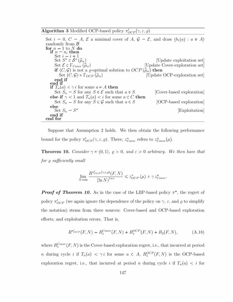
Algorithm 3 Modified OCP-based policy π1OCP pγ, ε, %q

Set i 0, C A, E a minimal cover of A, G E , and draw pb1paq : a P Aqrandomly from Bfor n 1 to N do

if n ni thenSet i i 1Set S P S ppµnq [Update exploitation set]Set E P ΓCover ppµnq [Update Cover-exploration set]if pC,Gq is not a %-optimal solution to OCP ppµnq then

Set pC,Gq P ΓOCP ppµnq [Update OCP-exploration set]end if

end ifif Tnpaq γ i for some a P A then

Set Sn S for any S P E such that a P S [Cover-based exploration]else if γ 1 and Tnpaq i for some a P C then



end for

Suppose that Assumption 2 holds. We then obtain the following performance

bound for the policy π1OCP pγ, ε, %q. There, zCover refers to zCoverpµq.

Theorem 10. Consider γ P p0, 1q, % ¡ 0, and ε ¡ 0 arbitrary. We then have that

for % sufficiently small

limNÑ8

Rπ1OCP pγ,ε,%qpF,Nq

plnNq1ε¤ zOCP pµq γ zCover.

Proof of Theorem 10. As in the case of the LBP-based policy π, the regret of

policy π1OCP (we again ignore the dependence of the policy on γ, ε, and % to simplify

the notation) stems from three sources: Cover-based and OCP-based exploration

efforts, and exploitation errors. That is,

Rπ1OCP pF,Nq RCover1 pF,Nq ROCP

1 pF,Nq R2pF,Nq, (A.18)

where RCover1 pF,Nq is the Cover-based exploration regret, i.e., that incurred at period

n during cycle i if Tnpaq γ i for some a P A, ROCP1 pF,Nq is the OCP-based

exploration regret, i.e., that incurred at period n during cycle i if Tnpaq i for

147

some a P C, and R2pF,Nq is the exploitation-based regret, i.e., that incurred when

exploration conditions are met and one implements solution Sn S with S P

Sppµnq.We prove the result by bounding each term in (A.18) separately. It turns out

that the bounds for RCover1 pF,Nq and R2pF,Nq in Step 1 and Step 2.1 in the proof

of Theorem 6 apply to this setting unmodified, thus we omit them here. Next, we

bound the OCP-based exploration regret ROCP1 pF,Nq.

As in the proof of the LBP-based policy, in the remainder of this proof, E and

P denote expectation and probability when costs are distributed according to F and

policy π1OCP is implemented.

Step 2.2’ (OCP-based exploration regret).

Following the arguments in Step 2.2 of the proof of Theorem 6, we first define

the minimum precision threshold on the accuracy of mean cost estimates necessary

to reconstruct the solution to OCP pµq. For that, we define

∆D : min ∆µmin,∆

D2 ,∆

D3 ,∆

D4

(p8scq,

where

∆D2 : min

!min

!∆pµ^lqpDqS : S R S ppµ^ lq pDqq

): D AzH, S pµq S ppµ^ lq pDqq

),

∆D3 : min tzCombpµq zComb ppµ^ lq pDqq : D AzH, S pµq S ppµ^ lq pDqqu ,

∆D4 : min

#¸SPG

∆µS

zOCP pµq : pC,Gq P GzΓOCP pµq

+,

and G denotes the set of all feasible solutions pC,Gq to OCP pµq problem. Note that

as in the proof of Theorem 6, ∆µmin min t∆µ

S : S P SzS pµqu, s max t|S| : S P Su,

c max t|E | : E P Cu, i.e., the maximum size of a minimal cover of A, and H SPSpµq

aPS tau. Also note that ∆D

4 denotes the minimum optimality gap of

problem OCP pµq. Note that thresholds ∆µmin, ∆D

2 and ∆D4 are always positive,

while ∆D3 ¡ 0 by Assumption 2.

148

We now check that having mean cost estimates with enough precision allows to

reconstruct the feasible set G. Consider px, yq satisfying (2.7b) and (2.7d). We first

note that as discussed in Step 1 of the proof of Theorem 6, tpµn µ8 ∆µminp2squ

ensures that tSppµnq Spµqu. One then has that

!pµn µ8 ∆

D)

# ¸aPS

xpaq ppµnpaq µpaqq

∆Ds, @S P S

+X

!zCombppµnq zCombpµq

∆Ds)

# ¸aPS

pxpaqpµnpaq p1 xpaqqlpaqq zCombppµnq

¸aPS

pxpaqµpaq p1 xpaqqlpaqq zCombpµq

2∆Ds, @S P S

+.

We conclude that, because 2∆Ds ∆D2 ^∆D

3 ,

¸aPS

pxpaqµpaq p1 xpaqqlpaqq ¥ zCombpµq iff¸aPS

pxpaqpµnpaq p1 xpaqqlpaqq ¥ zCombppµnq.

Having the same feasible region for both OCP pµq and OCP ppµnq problems, we

now show that %-optimal solutions to the latter problem corresponds to an optimal

solution to the former. Indeed, we have that

pµn µ8 ∆D(

"∆pµnS ∆µ

S

∆D4

4c, @S P S

*

#¸SPG

∆pµnS ∆µ

S

∆D4

4, @pC,Gq P G

+

#¸SPG

∆pµnS ¡ ∆D

4 2¸SPG

∆pµnS , @pC,Gq P ΓOCP pµq , pC,Gq P GzΓOCP pµq

+.

The above not only implies that ΓOCP ppµnq ΓOCP pµq, but also that %-optimal

solutions to OCP ppµnq are also optimal to OCP pµq, as long as % ∆D4 2. Letting

Γ%OCP pνq denote the set of %-optimal solutions to OCP pνq, the above implies that for

% ∆D4 2,

pµn µ8 ∆D( tΓ%OCP ppµnq ΓOCP pµqu .

149

We are now ready to provide a bound on ROCP1 pF,Nq. Similar to the proof of

Theorem 6, let i1 be a finite upper bound on a cycle in which one is sure to conduct

all OCP-based explorations (e.g., i1 : 1 inf ti P N, i ¥ 2 : ni1 ni ¡ i |A|u). Fix

i ¡ i1 and let pCi,Giq denote the OCP-based exploration set for any period n P

rni, ni1 1s. Define the events Ξ1i : tpCi,Giq P ΓOCP pµqu and Ξ2

i : tGi Gi1u.

We then have that

ROCP1 pF,Nq ¤ ni11∆µmax

rplnNq1εs¸ii11

E

#1 Tni1paq ¥ γpi 2q , @a P A ,

Ξ1i X Ξ2

i

( ¸SPGi

∆µS

+

rplnNq1εs¸ii11

i E

#1!Tni1paq ¥ γpi 2q , @a P A ,

Ξ1i X Ξ2

i

c) ¸SPGi

∆µS

+

¤ ni11∆µmax

plnNq1ε 1

zOCP pµq

∆µmax c

8

ii11

i P!Tni1paq ¥ γpi 2q , @a P A ,

Ξ1i X Ξ2

i

c), (A.19)

where pΞ1i X Ξ2

i qc

denotes the complement of the event pΞ1i X Ξ2

i q. Next, we bound

the probability inside the sum in (A.19). For that, observe that

pµni1

µ8 _ pµni µ8 ∆D( Γ%OCP ppµni1

q ΓOCP pµq(

X tΓOCP pµq Γ%OCP ppµniquΞ1i X Ξ2

i

.

Using above and Proposition 30, we conclude that

P Tni1

paq ¥ γpi 2q , @a P A ,Ξ1i X Ξ2

i

c(¤ 4 |A| exp

#

2∆D

2γpi 2q

L2

+.

(A.20)

Using the above and (A.19), we have that

ROCP1 pF,Nq ¤ plnNq1ε zOCP pµq C5,

for a finite positive constant C5, independent of N . Putting the results from Steps 1

150

and 2.1 (from the proof of Theorem 6), and Step 2.2’ together, we conclude that

Rπ1OCP pF,Nq ¤ pzOCP pµq γ zCoverpµqq plnNq1ε C6,

for a finite positive constant C6, independent of N .

We finally note that the optimal solutions to the Coverppµniq and OCP ppµniqproblems converge a.s. to optimal solutions to Coverpµq and OCP pµq, respectively.

For this, note that Proposition 30, (A.13) and (A.20) imply (via Borel-Cantelli) that

P tEi P ΓCoverpµq e.v.u 1 and

P tpCi,Giq P ΓOCP pµq e.v.u 1.


A.3.1 General Complexity of OCP

To prove Theorem 11 and Proposition 12, we will use the following lemma.

Lemma 31. We may restrict the OCP or Cover problems to have at most |A|

non-zero ypSq variables without changing the problems.

Proof of Lemma 31. For the OCP problem, the result follows from noting that

any critical set C can be covered by at most |A| solutions (i.e., by a solution-cover

G of at most size |A|). Hence, if an optimal solution for OCP has |G| ¡ |A|, we may

remove one solution from it while preserving feasibility. If the removed solution is

suboptimal for Comb, we would obtain a solution with lower objective value contra-

dicting the optimality for OCP . If the removed solution is optimal for Comb, we

obtain an alternate optimal solution for OCP .

For the Cover problem, the result follows by noting that A can be covered by at

most |A| solutions.

151

Theorem 11. If Comb is in P, then OCP is in NP.

Proof of Theorem 11. By Lemma 31, optimal solutions to OCP and Cover have

sizes that are polynomial in |A| and their objective function can be evaluated in

polynomial time. Checking the feasibility of these solutions for OCP can be achieved

in polynomial time, because checking (2.7c) can be achieved by solving Combpνxq

where νx : pνxpaq : a P Aq for νxpaq : lpaqp1 xpaqq νpaqxpaq. This problem is

polynomially solvable by assumption.

A.3.2 Critical Sets for Matroids

Lemma 32. Let Combpνq be a weighted basis or independent set matroid minimiza-

tion problem. Then there exists a unique critical set that can be found in polynomial

time.

Proof of Lemma 32. To simplify the exposition, we assume that S pνq tSu

is a singleton. Also, for S P S, we let eS denote the incidence vector associated with

S (i.e., eS : peSpaq : a P Aq with eSpaq P t0, 1u, a P A, is such that eSpaq 1 if

a P S and eSpaq 0 otherwise).

Let P : conv eS(SPS

R|A| be the independent set (base) polytope of S.

Then, for ν feasible, S P S pνq if and only if°aPS νpaq ¤

°aPS νpaq for any S P S

such that eS

and eS are adjacent vertices in P . Furthermore, each adjacent vertex

to eS

can be obtained from S by: removing (denoted by “R”), adding (denoted

by “A”), or exchanging (denoted by “E”) a single element of S (Schrijver, 2003,

Theorem 40.6). Thus, we construct the set C so that S is always optimal if and

only if the cost of all elements of C are at their expected value. The construction

procedure starts with C S. In some steps we distinguish between S corresponding

to independent sets or bases.

R. (for the independent set case) From the optimality of S, removing an element

152

never leads to optimality.

A. (for the independent set case) For each a P AzS such that S Y tau is an

independent set, if lpaq 0, then add a to C.

E. (for both cases) For each a P AzS, add a to C if

lpaq max tνpa1q : a1 P S, S Y tau z ta1u is an independent set (base)u .

By construction, covering all elements in C guarantees optimality of S, and

not covering some guarantees that S is no longer optimal. Note that the set C is

unique. For the case of multiple optimal solutions we simply repeat this procedure

for each one. Finally, the only computationally non-trivial step in the construction

of C is checking that this set is an independent set or a base, which can be done in

polynomial time.

A.3.3 Basic MIP Formulation for OCP

In this section we prove Proposition 12.

Proof of Proposition 12. For any feasible solution px, yq to (2.8), we have that x

is the incidence vector of a critical set. This, because (2.8d) enforces dual feasibility

of w when elements with xpaq 0 are not covered, and (2.8e) forces the objective

value of the dual of Combpν 1q to be greater than or equal to zCombpνq, where ν 1

diagplqp1xqdiagpνqx. With this, the optimal objective value of Combpν 1q is greater

than or equal to zCombpνq. On the other hand, any yi is the incidence vector of some

S P S because of (2.8c) and the assumptions on M and d. Finally, (2.8b) ensures

that the critical set is covered by the solution-cover (i.e., yi’s) induced by OCP .

Lemma 31 ensures that the |A| variables yi are sufficient for an optimal solution to

OCP . If less than |A| solutions are needed for the cover, then the optimization can

pick the additional yi variables to be the incidence vector of an optimal solution to

153

Combpνq so that they do not increase the objective function value. The extension

for Cover is straightforward.

A.3.4 IP Formulation for OCP when Combpνq Admits a Compact IP Formulation

Suppose Combpνq admits a compact IP formulation such that yS(SPS ty P

t0, 1u|A| : My ¤ du for some M P Rm|A| and d P Rm, where yS denotes the in-

cidence vector of S P S. For simplicity, we assume that A t1, . . . , |A|u. Then an

IP formulation of OCP pνq is given by

min¸iPA

¸aPA

νpaqyipaq zCombpνq

(A.21a)

s.t. xpaq ¤¸iPA

yipaq, a P A (A.21b)

Myi ¤ d, i P A (A.21c)¸aPS

plpaqp1 xpaqq νpaqxpaqq ¥ zCombpνq, S P S (A.21d)

xpaq, yipaq P t0, 1u , a, i P A. (A.21e)

As in formulation (2.8), a feasible solution px, yq to (A.21) is such that x is the

incidence vector of a critical set (this is enforced by (A.21d)), and the yi’s are a

cover of such set, due to (A.21b), (A.21c), and the assumptions on M and d. Note

that an efficient cover includes at most |A| solutions (the optimization can pick the

additional yi to be the incidence vector of an optimal solution).

Formulation (A.21) has a polynomial number of variables, but the number of

constraints described by (A.21d) is in general exponential. However, the computa-

tional burden of separating these constraints is the same as solving Combpνq (finding

a violated inequality (A.21d) or showing that it satisfies all these inequalities can be

done by solving Comb pν 1q for ν 1paq lpaqp1 xpaqq νpaqxpaq). Hence, if we can

solve Combpνq sufficiently fast (e.g., when the problem is in P, or it is a practi-

154

cally solvable NP-hard problem) we should be able to effectively solve (A.21) with

a branch-and-cut algorithm that dynamically adds constraints (A.21d) as needed.

Finally, note that a formulation for Cover is obtained by setting xpaq 1 for all

a P A and removing (A.21d).

A.3.5 Linear-sized Formulation of OCP for Shortest Path Problem

Let Combpνq correspond to a shortest s t path problem in a digraph G pV,Aq.

Define A A Y tpt, squ and let δout and δin denote the outbound and inbound arcs

in digraph G pV, Aq. An optimal solution px, p, wq to

min

¸aPA

νpaq ppaq

zCombpνq p ppt, sqq (A.22a)

s.t. xpaq ¤ ppaq, a P A (A.22b)¸aPδoutpvq

ppaq ¸

aPδinpvqppaq 0, v P V (A.22c)

wpuq wpvq ¤ l ppu, vqq p1 x ppu, vqqq ν ppu, vqqx ppu, vqq , pu, vq P A(A.22d)

wpsq wptq ¥ zCombpνq (A.22e)

ppaq P Z, a P A (A.22f)

xpaq P t0, 1u , wpvq P R, a P A, v P V, (A.22g)

is such that pC,Gq is an optimal solution to OCP pνq, where C ta P A : xpaq 1u

and G S is a set of paths for which ppaq |tS P G : a P Su|. Such a set G can be

constructed from p in time Op|A||V |q.

The first difference between formulations (A.22) and (2.8) is the specialization

of the LP duality constraints to the shortest path setting. The second one is the

fact that the paths in cover G are aggregated into an integer circulation in aug-

mented graph G, which is encoded in variables p. Indeed, using known properties

155

of circulations (Schrijver, 2003, pp. 170-171), we have that p °SPG y

S, where yS

is the incidence vector of the circulation obtained by adding pt, sq to path S. Fur-

thermore, given a feasible p we can recover the paths in G in time Op|A||V |q. To

obtain a formulation for Cover, we simply set xpaq 1 for all a P A and remove

(A.22d)–(A.22e).

It is possible to construct similar formulations for other problems with the well-

known integer decomposition property (Schrijver, 2003).

A.3.6 A Time-Constrained Asynchronous Policy

Depending on the application, real-time implementation might require choosing a

solution Sn P S prior to the exogenous arrival of the cost vector Bn. However,

the solution times for the problems OCP pq or even Combpq could be longer than

the time available to the executing policy. For example, most index-based policies

must solve an instance of Combpq at each period, which might not be possible in

practice. Fortunately, a key feature of our proposed OCP-based policies is that the

frequency at which the problems Combpq and OCP pq need to be solved decreases

exponentially. Indeed, such problems are solved at the beginning of each cycle and

the length of cycle i is Θ pexp piHqq for a fixed tuning parameter H ¡ 0. Hence, as

cycles elapse, there will be eventually enough time to solve these problems.

Nonetheless, the policy cannot proceed until the problems Combpq and OCP pq

are solved. However, one can easily modify the policy so that it begins solving

Combpq and OCP pq at the beginning of a cycle, but continues to implement in-

cumbent solutions while these problems are being solved (such solutions might be

computed either upfront or in previous cycles). Solutions to these problems update

incumbent solutions as they become available, which for long cycles would be at the

beginning of the next one. Algorithm 4 presents one such possible modification for

the OCP-based policy.

156

Algorithm 4 Basic Time-Constrained Asynchronous OCP-based policy πAOCP pHq

Set i 0, C A, and G a minimal cover of ALet S P S be an arbitrary solution and pµComb pµOCP be an initial cost estimateAsynchronously begin solving Comb ppµCombq and OCP ppµOCP qfor n 1 to N do

if n ni thenSet i i 1if Asynchronous solution to Comb ppµCombq has finished then

Set S P S ppµCombq [Update exploitation set]Set pµComb pµnAsynchronously begin solving Comb ppµCombq

end ifif Asynchronous solution to OCP ppµOCP q has finished then

Set pC,Gq P ΓOCP ppµOCP q [Update OCP-exploration set]Set pµOCP pµnAsynchronously begin solving OCP ppµOCP q

end ifend ifif Tnpaq i for some a P C then



end for

A.3.7 Greedy Oracle Polynomial-Time Heuristic

To further illustrate the potential practicality of policies based on OCP , we develop

a greedy heuristic for solving OCP that only requires a polynomial number of queries

to an oracle for Combpq (plus a polynomial number of additional operations). This

heuristic always returns a solution that is equal and possibly arbitrarily better than

a minimal cover of A.

We begin by describing the heuristic for solving OCP pνq in Algorithm 5. Given

a cost vector ν, the heuristic first sets all costs to their lowest possible values, and

successively solves instances of Comb, each time incorporating the incumbent so-

lution into the solution-cover G, adding its ground elements to the (critical) set

C, and updating the cost vector accordingly. The procedure stops when the feed-

back from C suffices to guarantee the optimality of the best solution (i.e., when

zCombpν1q ¥ zCombpνq). To achieve efficiency of such a feedback, the heuristic then

157

prunes elements in C that are not required to guarantee sufficiency of the feedback.

Algorithm 5 Oracle Polynomial-Time Heuristic

Set ν 1 : pν 1paq : a P Aq plpaq : a P Aq, G H, C H.while zComb pν

1q zComb pνq doSelect S P S pν 1q and set ν 1paq νpaq for all a P SG Ð G Y tSu and C Ð C Y S

end whilefor a P C do

if zComb ppν1 ^ lq ptauqq ¥ zComb pνq then

C Ð Cz tau and ν 1paq Ð lpaqend if

end for

Note that in each iteration of the first loop, Algorithm 5 calls an oracle for Comb

and adds at least one ground element to C. Similarly, in the second loop, the heuristic

calls such an oracle once for every element in C. Hence, the procedure calls such an

oracle at most 2 |A| times. Thus, the heuristic makes a linear number of calls to the

oracle for Comb. In particular, if Comb is in P, then the heuristic runs in polynomial

time.

The performance of the heuristic ultimately depends on the specifics of a setting.

For instance, in the setting of Example 1, the heuristic returns, in the worst case, a

solution with |G| k, which is of the order of a cover of A. In the setting of Example

2 on the other hand, the heuristic returns a solution with |G| 2 (in such a setting

a cover of A is of order k). It is not hard to identify settings where the heuristic

performs arbitrarily better than any cover of A.

We finally note that the heuristic in Algorithm 5 can be modified as follows for

solving the Cover problem: the first loop should be implemented while A C and

the second loop is no longer needed. The resulting set G provides a cover of A.

A.4 Additional Computational Results

In this section we provide the computational results for Examples 1, 2 and 28. Figure

A.2 depicts the average performance of different policies on Examples 1 (left), 2

158

(center) and 28 (right), respectively.

N100 600 1100 1600 2000

Reg

ret

50

100

150

200

N100 600 1100 1600 2000

Reg

ret

100

200

300

400

500

Extended UCB1+

UCB1+

Extended UCB1+

Lower Bound

OCP-based

Greedy-Heuristic

Lower BoundGreedy-Heuristic

OCP-based

UCB1+

N100 600 1100 1600 2000

Reg

ret

5

10

15

20

Greedy-Heuristic

UCB1+

OCP-based

Extended UCB1+

Figure A.2: Average performance of different policies on Examples 1 (left), 2(center) and 28 (right).

On Example 1, the OCP-based and Greedy-Heuristic policies perform signifi-

cantly better than the benchmark policies. The situation is essentially the same on

Example 2, only that this time Extended UCB1+ outperforms the UCB1+ policy.

There, the solution to OCP pµq is only of size 2, which helps our policies achieve the

best performance. (Note that for this setting, the Greedy-Heuristic tends to find the

actual optimal solution to OCP pµq even with unreliable estimates.) On Example 28,

the heuristic solution to OCP coincides with the minimum-regret cover of S, thus

the Greedy-Heuristic policy is outperformed by UCB1+ (note that this latter policy

rarely uses the arcs p2 and q2, since the costs of p1 and q1 are close to 0).

As we discussed before, the lower bound in Theorem 5 is asymptotic, so it is not

clear whether the lower bound is meaningful in the finite time. However, we plot the

lower bound for the three shortest path examples in Figure A.2. As can be noted

from the graph, in Examples 1 and 2, the lower bound is in fact meaningful and the

regret of the OCP-based and Greedy-Heuristic policies is much closer to the lower

bound than the other benchmark policies. In Example 28, however, the lower bound

is not meaningful, that is, the lower bound is larger than the regret of all policies as

it only provides an asymptotic lower bound on regret.

159

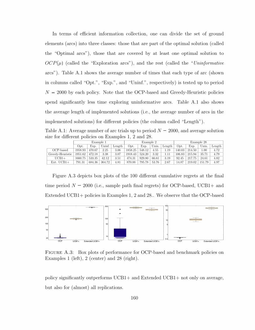
In terms of efficient information collection, one can divide the set of ground

elements (arcs) into three classes: those that are part of the optimal solution (called

the “Optimal arcs”), those that are covered by at least one optimal solution to

OCP pµq (called the “Exploration arcs”), and the rest (called the “Uninformative

arcs”). Table A.1 shows the average number of times that each type of arc (shown

in columns called “Opt.”, “Exp.”, and “Uninf.”, respectively) is tested up to period

N 2000 by each policy. Note that the OCP-based and Greedy-Heuristic policies

spend significantly less time exploring uninformative arcs. Table A.1 also shows

the average length of implemented solutions (i.e., the average number of arcs in the

implemented solutions) for different policies (the column called “Length”).

Table A.1: Average number of arc trials up to period N 2000, and average solutionsize for different policies on Examples 1, 2 and 28.

Example 1 Example 2 Example 28Opt. Exp. Uninf. Length Opt. Exp. Unin. Length Opt. Exp. Unin. Length

OCP-based 1958.93 470.67 2.25 3.06 1858.25 548.12 4.55 1.19 140.03 214.50 1.00 4.72Greedy-Heuristic 1951.62 472.18 3.38 3.07 1918.43 524.20 3.32 1.11 106.83 215.94 35.71 4.79

UCB1+ 1660.75 533.35 42.12 3.51 474.31 929.80 66.61 3.19 92.45 217.75 24.61 4.82Ext. UCB1+ 791.31 684.36 364.72 4.81 870.88 795.78 53.76 2.67 14.87 219.02 151.79 4.97

Figure A.3 depicts box plots of the 100 different cumulative regrets at the final

time period N 2000 (i.e., sample path final regrets) for OCP-based, UCB1+ and

Extended UCB1+ policies in Examples 1, 2 and 28.. We observe that the OCP-based

OCP UCB1+ Extended UCB1+

20

50

100

200

500

OCP UCB1+ Extended UCB1+

10

50

100

500

OCP UCB1+ Extended UCB1+0.5

1

5

10

50

100

Figure A.3: Box plots of performance for OCP-based and benchmark policies onExamples 1 (left), 2 (center) and 28 (right).

policy significantly outperforms UCB1+ and Extended UCB1+ not only on average,

but also for (almost) all replications.

160

A.5 Alternative Feedback Setting

The flexibility of the OCP-based policies allows them to be easily extended or com-

bined with other techniques that consider similar what-and-how-to-explore questions.

For instance, the OCP-based policy can be easily combined with the “barycentric

spanner” of Awerbuch and Kleinberg (2004) to extend our results from element-level

observations to set- or solution-level observations as follows. For a particular appli-

cation, it might be the case that the decision-maker only has access, for example,

to the total cost incurred by implementing solution Sn. We begin by showing how a

cover-based policy (i.e., a policy that conducts exploration by implementing solutions

in a cover) can be adapted to this last setting. For a set of ground elements S A,

let IS : pISpaq : a P Aq P t0, 1u|A| denote the incidence vector of the ground set (so

that S ta : ISpaq 1, a P Au). We say a solution set E recovers a set E A if for

each a P E, there exists a vector γpaq : pγSpaq, S P Eq P R|E| such that

¸SPE

γSpaqIS Itau. (A.23)

Without loss of generality, one can assume that each ground element is recovered

by at least one solution set. Let E be a solution set that recovers A, and let γ :

pγpaq, a P Aq be such that°SPE γSpaqIS Itau, for all a P A. One can implement a

cover-based policy with E playing the role of a cover while using the estimate mean

cost vector pµn ppµnpaq : a P Aq, where

pµnpaq :¸SPE

γSpaq

|m n : Sm S|

¸m n:SmS

¸aPS

bmpaq, a P A. (A.24)

The estimate above reconstructs the expected cost of each solution in E and uses

(A.23) to translate such estimates to the ground-element level. Implementing this

modification requires precomputing a solution set E recovering A. Such a set can be

161

selected so that |E | ¤ |A|, and computed by solving Op|A|q instances of Combpq (see

e.g., the algorithm in Awerbuch and Kleinberg (2004)).

The idea above can also be used to extend the OCP-based policy to this new

setting. For that we could consider the estimates in (A.24) and pC, Eq to be a

solution to an alternative version of OCP pνq, denoted by OCP 1pνq, where in addition

to (2.7b)-(2.7d), one imposes that E recovers C, that is, OCP 1pνq is given by

min¸SPS

∆νS ypSq (A.25a)

s.t.¸SPS

γSpaqIS xpaqItau, a P A (A.25b)

γSpaq ¤ Q ypSq, S P S, a P A (A.25c)

γSpaq ¤ Q ypSq, S P S, a P A (A.25d)¸aPS

plpaqp1 xpaqq bpaqxpaqq ¥ zCombpνq, S P S (A.25e)

xpaq, ypSq P t0, 1u , γSpaq P R, a P A, S P S, (A.25f)

where Q is an instance-dependent constant, whose size is polynomial in the size of

the instance. The additional constraints(A.25b)-(A.25d) in OCP 1pνq ensure that the

solution-cover E recovers the critical set C. Like OCP , the formulation above can be

specialized to accommodate the combinatorial structure of Comb. The performance

guarantee in Theorem 10 would remain valid with the constants associated with

OCP 1. We anticipate that the challenge of solving OCP 1 effectively is comparable

to that of solving OCP .

A.6 Auxiliary Result for the Proof of Theorem 6 and Theorem 10

In this section we prove Proposition 30 which we used in the proof of Theorem 6 and

Theorem 10.

162

Proof of Proposition 30. For m P N, define tmpaq : inf tn P N : Tnpaq mu1.

Indexed by m, one has that Btmpaqpaq µpaq is a bounded martingale difference

sequence, thus one has that

P t|pµnpaq µpaq| ¥ ε , Tnpaq ¥ ku P

$&%Tnpaq¸m1

Btmpaqpaq µpaq

¥ ε Tnpaq , Tnpaq ¥ k

,.-¤

8

hk

P

# h

m1

Btmpaqpaq µpaq

¥ ε h , Tnpaq h

+

paq¤ 2

8

hk

exp

"2 hε2

L2

*P tTnpaq hu

¤ 2 exp

"2 kε2

L2

*,

where paq follows from the Hoeffding-Azuma Inequality (see, for example, Lemma

A.7 in Cesa-Bianchi and Lugosi (2006)).

163

Appendix B


B.1 Proofs

Detailed Derivation of the approximate lower bound G1lpT,I 1q. We define

product j’s optimality gap for customers with profile i as ∆ij : maxt1¤l¤Nutµiluµ

ij

for j P N and i P I. Let kijptq denote the number of times that product j has been

offered to a customer with profile i up to (and including) time t. One can rewrite the

retailer’s regret associated with a policy π, defined in (3.3), as RπpT, Iq °Ii1R

πi pT q

where Rπi pT q is the regret associated with profile i and policy π:

Rπi pT q :

N

j1

∆ij Eπ

kijpT q

.

The regret is proportional to the number of times that suboptimal assortments are

offered to customers over the selling season.

In their seminal work, Lai and Robbins (1985a) proved that the regret of any

consistent policy in a classic bandit setting grows asymptotically with order at least

164

lnpT q. Formally, for any consistent policy π, we have that

lim infTÑ8

RπpT q

lnpT q¥

¸jPN :∆j¡0

∆j

Dj

, (B.1)

where ∆j is the optimality gap and Dj is the Kullback-Leibler divergence associated

with arm j P N .1

Because all profiles within a cluster have the same distribution of preferences,

with some abuse of notation, we let ∆kj denote the optimality gap of product j for

all profiles in cluster k; that is, ∆ij ∆k

j for all i P Ik where recall that Ik denotes

the set of profiles belonging to cluster k. Similarly, we let Dij Dk

j for all i P Ik.

Building on Lai and Robbins’ result in (B.1), we consider the following (asymptotic)

lower bound on the regret for the data-intensive policy:

Ld-intpT, I 1q :K

k1

N

j2

∆kj

Dkj

¸iPIk

E rlnpTiqs ,

where Ti is the (random) number of customers from profile i that arrive during the

selling season. Hence,°Ii1 Ti T almost surely.2 Note that Ld-int is the sum of the

lower bound on the regret associated with each profile (or cluster). Unlike the setting

studied in Lai and Robbins (1985a), which considers a homogeneous population of

customers, the number of customer arrivals from each profile (i.e, Ti) is random.

This introduces additional complexity in the computation of the lower bound, which

we address by using a first-order Taylor expansion of the term lnpTiq.3 We therefore

1 The Kullback-Leibler divergence measures the difference between two probability distributions.For the Bernoulli distribution, we have Dj : µj lnpµjµ

q p1 µjq lnpp1 µjqp1 µqq, whereµ : maxjPN tµju.

2 Although the lower bound in (B.1) is attained when T Ñ 8, one can obtain a similar lowerbound on the regret associated with each profile i, Rπi pT q, as Ti Ñ 8. This is because Ti Ñ 8almost surely as T Ñ8, as long as pi ¡ 0 for each profile i P I.

3 In deriving the bounds, we use a first-order Taylor expansion which, as one may expect, providesa reasonable approximation for smooth functions – we also verified this numerically.

165

approximate Ld-int by replacing lnpTiq by its first-order Taylor expansion around the

mean EpTiq piT . To this end, we have that lnpTiq lnppiT q p1ppiT qqpTi piT q

and taking expectation on both sides, we have that E rlnpTiqs lnppiT q as EpTiq

piT . Thus, we approximate the lower bound function Ld-int with Lapxd-int where

Ld-intpT, I 1q Lapxd-intpT, I1q :

K

k1

N

j2

∆kj

Dkj

¸iPIk

lnppiT q.

Using the results in Auer et al. (2002) for the UCB1 policy, an upper bound on

the regret for the semi-oracle policy is given by:

Us-orcpT, I 1q :K

k1

N

j2

8

∆kj

E rlnpT 1kqs

1

π2

3

N

j2

∆kj

,

where T 1k denotes the (random) number of customers from cluster k. Using a similar

first-order Taylor expansion as in Lapxd-int, we approximate the upper bound function

Us-orc with Uapxs-orc where

Us-orcpT, I 1q Uapxs-orcpT, I 1q :

K

k1

N

j2

8

∆kj

lnpPkT q

1

π2

3

N

j2

∆kj

,

where Pk :°iPIk pi.

We therefore approximate the lower bound function Ld-intpT, I 1qUs-orcpT, I 1q by

G1lpT, I 1q : Lapxd-intpT, I1q Uapx

s-orcpT, I 1q.

Since the gap function can be defined as the gap associated with each cluster, we

further define G1lpT, I 1q °Kk1G

k1lpT, Ikq where

Gk1lpT, Ikq :

N

j2

∆kj

Dkj

¸iPIk

lnppiT q

N

j2

8

∆kj

lnpPkT q

1

π2

3

N

j2

∆kj

.

166

The next result provides conditions under which G1lpT, I 1q ¥ 0.

Theorem 33. For each k P t1, . . . , Ku, suppose that Ik ¥ Ikl for some Ikl independent

of T and of the distribution of customer arrivals. Then, piq there exist thresholds

tkl pIkq such that G1lpT, I 1q ¥ 0 for T ¥ maxk tkl pIkq

(; and piiq G1lpT, I 1q is increasing

and concave in T .

Proof. piq To prove that G1lpT, I 1q ¥ 0, we first characterize conditions under which

Gk1lpT, Ikq ¥ 0. After some algebra, we obtain that

Gk1lpT, Ikq A lnpT q B,

where A : Ik

°Nj2 ∆k

j Dkj

°Nj2 8∆k

j ,

B :

N

j2

∆kj D

kj

ln

¹iPIk

pi

N

j2

8∆kj

lnpPkq

1 π23

N

j2

∆kj ,

Pk °iPIk pi, and Dk

j is the Kullback-Leibler divergence number. Let Ikl be the

smallest integer greater than°N

j2 8∆kj

°N

j2 ∆kj D

kj

and set Ik ¥ Ikl . Note

that A ¡ 0 for Ik ¥ Ikl . We therefore have that Gk1lpT, Ikq ¥ 0 if

T ¥ tkl pIkq : rexppBAqs.

The result follows from noting that G1lpT, I 1q °Kk1G

k1lpT, Ikq.

piiq This part follows immediately as G1lpT, I 1q °Kk1G

k1lpT, Ikq where Gk

1lpT, Ikq

A lnpT q B (where A and B are as defined in part piq), and A ¡ 0 for Ik ¥ Ikl .

As expected, the semi-oracle outperforms the data-intensive policy as it learns

about customers’ preferences faster by pooling information across customer profiles

within any cluster. The requirement of sufficiently large Ik in Theorem 33 is mostly

technical and emerges from the mismatch between the leading constants in the lower

167

and upper bounds to the regret functions. On the other hand, the requirement on

T ensures that the number of customers in each profile is not too small with high

probability. Theorem 33piiq shows that G1lpT, I 1q is increasing (and, in fact, grows

to infinity) in the number of arriving customers T .

Proof of Theorem 13. We assume for simplicity that Ik is continuous. The results

follow directly for the discrete case. We prove the results by taking the first- and

second-order partial derivatives. We first prove that BG1lpT, I 1qBIk ¡ 0. We have

that ln±

iPIk pi Ik lnpPkq Ik lnpIkq. Then,

BG1lpT, I 1qBIk

N

j2

∆kj

Dkj

plnpT q lnpPkq lnpIkq 1q .

Note that BG1lpT, I 1qBIk ¡ 0 if T ¡ eIkPk. To prove concavity, note that

B2G1lpT, I 1qBIk

2

N

j2

∆kj

Dkj

1

Ik

0.

168

Detailed Derivation of the approximate lower bound G2lpT, I, P q. We as-

sume that ∆kj ∆ ¡ 0 for all k 1, . . . , K and j k, where recall that ∆k

j de-

notes the optimality gap of product j for all profiles in cluster k. Similarly, we let

Dkj D ¡ 0 for all k 1, . . . , K and j k, where Dk

j denotes the Kullback-Leibler

divergence associated with product j for all profiles in cluster k. As in derivation of

the approximate lower bound G1lpT, I 1q, we consider the (asymptotic) lower bound

on the regret of the data-intensive policy:

Ld-intpT, I, P q :pK 1q∆

D

I

i1

E rlnpTiqs .

Existing upper bounds in the bandit literature (including that of the UCB1 policy)

assume a homogeneous market. This introduces additional complexity in the com-

putation of the upper bound on the regret of the pooling policy, which we address

in the following result.

Lemma 34. The regret for the pooling policy in this setting is at most

UpoolpT, I, P q

8 lnpT q

∆

K

k2

1

P1 Pk

1

π2

3

pKP1 1q∆

T p1 P1q∆.

Note that Upool in Lemma 34 has an additional term compared to its counterpart

in the case of a homogeneous market. The term inside square brackets is the upper

bound on the regret of the pooling policy relative to a “weak” oracle. The “weak”

oracle assumes that the market is homogeneous and therefore always offers product

1 (as it has a higher purchase probability averaged over all customer profiles) to

any arriving customer. However, the regret has to also account for the pooling

policy’s inability to differentiate between clusters. The term outside square brackets

incorporates such a penalty. Note that this penalty term disappears as P1 Ò 1.

169

Let G2lpT, I, P q be the approximation of the lower bound Ld-intUpool, obtained

by replacing lnpTiq with its first-order Taylor expansion. That is,

G2lpT, I, P q :pK 1q∆

D

I

i1

lnppiT q

8 lnpT q∆

K

k2

1

P1 Pk

T p1 P1q∆

1 π2

3

pKP1 1q∆

.

Proof of Lemma 34. We construct Upool in two steps. First, consider a “weak”

oracle that assumes that the market is homogeneous, and therefore, presumes that

the purchase probabilities are P1µ1jP2µ

2j PKµ

Kj for each product j, where µkj

denotes the purchase probability of product j for cluster k. Because the optimality

gap of products in all clusters is the same (i.e., ∆kj ∆ for any cluster k and product

j k) and P1 ¡ max tP2, . . . , PKu, the weak oracle offers product 1 to all arriving

customers regardless of their profiles (or clusters). As a result, the optimality gap of

product k 2, . . . , K (averaged over all profiles) for the weak oracle is:

∆1k : pP1µ

11 P2µ

21 PKµ

K1 q pP1µ

1k P2µ

2k PKµ

Kk q pP1 Pkq∆ ¡ 0.

If the pooling policy follows the UCB1 algorithm of Auer et al. (2002) (which assumes

a homogeneous market), its regret relative to the weak oracle is at most

K

k2

8 lnpT q

∆1k

1

π2

3

∆1k

8 lnpT q

∆

K

k2

1

P1 Pk

1

π2

3

pKP1 1q∆.

The pooling policy’s regret, however, has to also account for its inability to differ-

entiate between clusters. Now, consider a “strong” oracle that knows the purchase

probabilities of all customer profiles (and thus the mapping of profiles to clusters).

The strong oracle offers product k to customers from cluster k for k 1, . . . , K,

while the weak oracle offers product 1 to all arriving customers regardless of their

profiles (or clusters). As a result, the weak oracle incurs an additional cost (regret)

170

relative to the strong oracle whenever a customer from a cluster other than cluster

1 arrives. Hence, the weak oracle’s regret relative to the strong oracle due to the

lack of knowledge of the mapping of profiles to clusters is T p1P1q∆. Therefore, we

obtain

UpoolpT, I, P q

8 lnpT q

∆

K

k2

1

P1 Pk

1

π2

3

pKP1 1q∆

T p1 P1q∆.

Proof of Theorem 14. Note that if P1 1, this setting coincides with a homoge-

neous market and thus the results follow from Theorem 33. Therefore, we prove the

results for P1 1.

We first characterize conditions under which G2lpt, I, P q ¥ 0. For simplicity we

assume that t is continuous, but similar arguments apply to the discrete case. After

some algebra, we obtain that

G2lpt, I, P q A1 lnptq B1t C 1,

where A1 : pK 1qI∆D 8β∆, B1 : p1 P1q∆,

C 1 : ppK 1q∆Dq ln

I¹i1

pi

1 π23

pKP1 1q∆,

β :°Kk2 1 pP1 Pkq, and D is the Kullback-Leibler divergence. Note that if

A1 ¤ 0, then G2lpt, I, P q 0 for all t ¥ 1 as B1 ¡ 0 and C 1 ¡ 0. Thus, we need

A1 ¡ 0 which requires that

I ¡8βD

pK 1q∆2. (B.2)

Having A1 ¡ 0 implies that G2lpt, I, P q is a concave function of t, and this function

has a maximum at t A1B1. Let Gmaxl : maxt¡0 tG2lpt, I, P qu G2lpA

1B1, I, P q.

171

Note that BG2lpt, I, P qBt ¥ p q 0 for t ¤ p¡q A1B1, and G2lpt, I, P q Ñ 8 as

t Ñ 8 (since B1 ¡ 0). Therefore, if Gmaxl ¡ 0, we have that G2lpt, I, P q ¥ 0 for

tlpI, P q ¤ t ¤ tupI, P q for some thresholds 1 tlpI, P q ¤ tupI, P q ¤ 8. In what

follows, we provide conditions that guarantee that Gmaxl ¡ 0. We have that

Gmaxl A1 lnpA1B1q A1 C 1.

It follows that Gmaxl ¡ 0 if

A1

B1 ¡ exp

C 1

A1 1

. (B.3)

Considering the fact that arrivals are uniform, i.e., pi 1I,@i, we have that

ln±I

i1 pi

I lnpIq. This implies that

C 1

A1 ppK 1q∆Dq I lnpIq p1 π23q pKP1 1q∆

pK 1qI∆D 8β∆

lnpIq p8β∆q lnpIq p1 π23q pKP1 1q∆

pK 1qI∆D 8β∆

lnpIq fpI, P q,

where

fpI, P q :p8β∆q lnpIq p1 π23q pKP1 1q∆

pK 1qI∆D 8β∆.

Therefore, to ensure that (B.3) holds, we provide conditions that guarantee that

A1

B1 ¡ expplnpIq fpI, P q 1q pexppfpI, P q 1qq I. (B.4)

After some algebra, we obtain that (B.4) is true if

K 1

p1 P1qD exppfpI, P q 1q

I ¡

8β

p1 P1q∆2. (B.5)

172

Note that for the above inequality to hold, the left-hand side of (B.5) must be

positive. This requires that P1 ¡ Π1pI, P q where

Π1pI, P q : 1K 1

D exppfpI, P q 1q.

For any given I and P 1, we let P1pI, P1q : inftP1 : P1 ¡ Π1pI, P q,max tP2, . . . , PKu

P1 1u where PK 1 pP1 P2 PK1q and recall that P 1 pP2, . . . , PK1q.

Note that Π1pI, P q 1. Moreover, in what follows (Lemma 35), we show that

fpI, P q (and thus Π1pI, P q) is decreasing in P1 for I ¡ e. Therefore, such P1pI, P1q

exists for I ¡ e. It follows that, if P1 ¡ P1pI, P1q and I ¡ e, then after some algebra

we have that (B.5) is true if

I ¡8βD

∆2 ppK 1q exppfpI, P q 1qp1 P1qDq. (B.6)

We now present the intermediate result.

Lemma 35. fpI, P q is decreasing in I and P1 (assuming that the vector P 1 is con-

stant) for I ¡ e.

Proof. We prove the result by taking the first-order partial derivatives. We have that

Bf

BI

8pK 1qβD p8β∆q2p1Iq ppK 1q∆Dq

p8β∆q lnpIq

1 π23

pKP1 1q∆

ppK 1qI∆D 8β∆q

2

rp8pK 1qβDq p1 lnpIqqs p8β∆q

2p1Iq

1 π23

pK 1qpKP1 1q∆2D

ppK 1qI∆D 8β∆q2 .

Note that p8pK 1qβDq p1 lnpIqq 0 guarantees that BfBI 0. The former

inequality holds if I ¡ e.

We note that PK 1 pP1 P2 PK1q. We then have that

Bβ

BP1

1

pP1 P2q2

1

pP1 P3q2

1

pP1 PK1q2

2

p2P1 P2 P3 PK1 1q2

0.

173

Thus, β is decreasing in P1 which implies that the denominator of function f is

increasing in P1. Therefore, to show that function f is decreasing in P1, we provide

conditions that guarantee that its numerator is decreasing in P1. Let fnum denote

the numerator of function f . We then have that

BfnumBP1

p8 lnpIq∆q γ K1 π23

∆,

where γ : BβBP1. Therefore, BfnumBP1 0 if

lnpIq ¡K p1 π23q∆2

8γ.

Since γ ¥ K, we have that I ¡ exp pp1 π23q∆28q guarantees that BfBP1 0.

Because expp1q e ¡ exp pp1 π23q∆28q as 0 ∆ ¤ 1, we conclude that I ¡ e

guarantees that BfnumBP1 0.

We conclude that in order to have Gmaxl ¡ 0, we need that P1 ¡ P1pI, P

1q and

the inequalities (B.2) and (B.6) to hold. Seeing that the right-hand side of inequality

(B.6) is larger than that for inequality (B.2), for any given P , we set IlpP q to be

the smallest integer I greater than e that satisfies the inequality (B.6) and take

I ¥ IlpP q. From Lemma 35, we know that fpI, P q is decreasing in I for I ¡ e.

Because the right-hand side of the inequality (B.6) is increasing in fpI, P q (and thus

decreasing in I for I ¡ e), such IlpP q exists (note that the right-hand side of the

inequality (B.6) converges to 8βD p∆2ppK 1q p1 P1qeDqq as I Ñ 8). This

completes the proof of G2lpt, I, P q ¥ 0.

We next prove that IlpP q is non-increasing in P1 (assuming that the vector P 1 is

constant). We know that IlpP q is the smallest integer I greater than e that satisfies

the inequality in (B.6). The result follows from noting that the right-hand side of

inequality (B.6) is decreasing in P1 for I ¡ e as a result of Lemma 35.

174

We finally prove that P1pI, P1q is non-increasing in I. We have from above that

P1pI, P1q inf tP1 : P1 ¡ Π1pI, P q,max tP2, . . . , PKu P1 1u ,

where Π1pI, P q 1 pK 1qpD exppfpI, P q 1qq. The result follows from noting

that Π1pI, P q is decreasing in I for I ¡ e as a result of Lemma 35.

175

B.2 Additional Proofs and Numerical Results

Extension of Theoretical Results for Thompson Sampling. Consider a clas-

sic bandit setting with N arms and Bernoulli rewards and suppose, without loss of

generality, that arm 1 is the unique optimal arm. Let ∆j denote the optimality gap

of product j. Agrawal and Goyal (2011) prove the following upper bound on the

regret of Thompson Sampling policy in this setting:

RπpT q ¤ C1 lnpT q C2,

where π denotes the Thompson Sampling policy,

C1 : 1152

N

j2

1

∆2j

2

288N

j2

1

∆2j

72N

j2

1

∆j

and

C2 : 192NN

j2

1

∆2j

104pN 1q.

Using the upper bound above, extending the results of Section 3.6.1 is immediate.

In what follows, we discuss the changes to the proof of Lemma 34 and Theorem 14.

Following the same arguments as in the proof of Lemma 34, we have in this setting

that

UpoolpT, I, P q pC 11 lnpT q C 1

2q T p1 P1q∆,

where

C 11 : 1152

K

k2

1

∆1k

2

2

288K

k2

1

∆1k

2 72K

k2

1

∆1k

and

C 12 : 192N

K

k2

1

∆1k

2 104pN 1q,

176

and ∆1k pP1 Pkq∆ is as defined in the proof of Lemma 34. After some algebra,

we obtain that

G2lpt, I, P q A1 lnptq B1t C 1,

whereA1 : pK 1qI∆DC 11, B1 : p1P1q∆, C 1 : ppK 1q∆Dq ln

±Ii1 pi

C 12. Following the same arguments as in the proof of Theorem 14, we need A1 ¡ 0

which requires that

I ¡C 1

1D

pK 1q∆. (B.7)

The only changes to the rest of the proof are the definitions of the functions fpI, P q

and IlpP q, and inequality (B.6). In this setting, we have that

fpI, P q :C 1

1 lnpIq C 12

pK 1qI∆D C 11

.

After some algebra, we have that the inequality (B.6) in this setting becomes

I ¡C 1

1D

∆ ppK 1q exppfpI, P q 1qp1 P1qDq. (B.8)

Similar to the proof of Theorem 14, we note that the right-hand side of inequality

(B.8) is larger than that for inequality (B.7). Thus, we define IlpP q as the smallest

integer I greater than e that satisfies the inequality in (B.8).

To conclude the extension, we only need to prove Lemma 35 in this setting.

Following the same arguments as in the proof of Lemma 35, we have that

Bf

BIrpC 1

1pK 1q∆Dq p1 lnpIqqs C 11

2I ppK 1q∆C 12Dq

ppK 1qI∆D C 11q

2 .

Note that I ¡ e guarantees that BfBI 0. To show that fpI, P q is decreasing

in P1, note that ∆1k is increasing in P1 which, in turn, implies that C 1

1 and C 12 are

decreasing in P1.

177

The non-increasing property of IlpP q and P1pI, P1q in P1 and I, respectively,

follows from similar arguments as in the proof of Theorem 14 and the discussion

above.

Details of Numerical Study in Section 3.5.5. The separation-based experiments

are discussed at the end of Section 3.5.5. Table B.1 below reports the percentage

improvement of the dynamic clustering policy over the other policies, both in terms

of regret and revenue (i.e., expected number of transactions) in the separation-based

experiments using a synthetic linear dataset.

Table B.1: Average percentage improvement of dynamic clustering policy over data-intensive and linear-utility policies in separation-based experiments using a syntheticlinear dataset.

Regret RevenueLinear-Utility Data-Intensive Linear-Utility Data-Intensive

T 500 31.2% 42.4% 26.2% 51%T 1000 33.4% 50% 20.3% 51%T 5000 36.4% 56% 11.1% 28.5%T 10000 16.7% 47.1% 3.3% 16.7%T 20000 -21.3% 34.4% -2.5% 8.5%

178

Appendix C


C.1 Proofs

Proof of Proposition 15. Considering the first-order condition (FOC) of π0ppq

with respect to p, after some algebra we have that

Bπ0ppq

Bp

exp ppβ pqµ1q pφ0ppq pq

pexppβµ1q expppµ1qq2 µ1

0,

where φ0ppq µ1 p1 exp ppβ pqµ1qq. Root of the above equation can be found

by either setting p 8, or by setting φ0ppqp 0. One can easily see that φ0ppq is a

decreasing function of p, and that φ0pp 0q ¡ 0 and φ0ppq Ñ µ1 as pÑ 8. Thus, the

equation φ0pp0q p0 has a unique solution at a finite price 0 p0 8. Therefore,

the FOC only holds at p p0 and p 8. We also note that Bπ0ppqBp ¡ 0 for

0 ¤ p p0 and Bπ0ppqBp 0 for p ¡ p0 . Thus, π0ppq is increasing (decreasing) in p

for p smaller than (larger than) p0 . Finally, we note that π0pp 0q 0, π0ppq Ñ 0

as p Ñ 8, and π0ppq is finite for all finite values of 0 p 8. These imply that

π0ppq is a unimodal function of p with a maximum at the optimal price 0 p0 8.

179

Replacing p0 by φ0pp0q in π0ppq, we obtain that

π0 π0pp0q p0 µ1 µ1 exp

β p0µ1

.

Proof of Proposition 16. From the Envelope Theorem and after some algebra,

we have that

Bπ0Bβ

Bπ0

Bβ

pp0

1

1 expβp0µ1

¡ 0.

Thus, π0 is increasing in β. To see that p0 is increasing in β, we note from the proof

of Proposition 15 that φ0ppq µ1p1 exp ppβ pqµ1qq, which is increasing in β.

Thus, the optimal price p0 which is the unique solution to φ0pp0q p0 is increasing

in β.

Proof of Proposition 17. Considering the FOC of π1ppq with respect to p, after

some algebra we have that Bπ1ppqBp 0 by either setting p 8, or by setting

φ1ppq p 0 where

φ1ppq

exp

βcµ2

exp

pµ2

exp

kµ1

expcµ2

exp

βpµ2

µ2µ1µ1µ2

exppµ2

exp

kµ1

expcµ2

exp

βpµ2

µ2µ1µ1 exp

kµ1 βc

µ2

µ2

.

Let C1 :

expcµ2

exp

βpµ2

µ2µ1. We then have that

Bφ1ppq

Bp

expbcpµ2

exp

kµ1

C1

µ1

C1µ1 exp

kµ1

pµ1 µ2q

exp

kµ1

2pβcqµ2

C1µ

22

exppµ2

exp

kµ1

C1

µ1 exp

kµ1

βcµ2

µ2

2 .

Because µ1 ¥ µ2, we can see from above that Bφ1ppqBp 0 for all p ¥ 0, that is, the

function φ1ppq is decreasing in p. We can also see that φ1pp 0q ¡ 0 and φ1ppq Ñ µ2

as p Ñ 8. Thus, the equation φ1pp1q p1 has a unique solution at a finite price

180

0 p1 8. Therefore, the FOC only holds at p p1 and p 8. One can also

check that Bπ1ppqBp ¡ 0 for 0 ¤ p p1 and Bπ1ppqBp 0 for p ¡ p1 . Thus, π1ppq

is increasing (decreasing) in p for p smaller than (larger than) p1 . Finally, we note

that π1pp 0q 0, π1ppq Ñ 0 as p Ñ 8, and π1ppq is finite for all finite values of

0 p 8. These imply that π1ppq is a unimodal function of p with a maximum at

the optimal price 0 p1 8. Replacing p1 by φ1pp1q in π1ppq, we obtain that

π1 π1pp1 q

µ1µ2 expβcµ2

exp

cµ2

exp

βp1µ2

µ2µ1

µ1 expp1µ2

exp

cµ2

exp

βp1µ2

µ2µ1

exppkµ1q

µ2 exppkµ1q exp

βcµ2

.


we have that

Bπ1Bβ

Bπ1

Bβ

pp1

exp

βcµ2

exp

cµ2

exp

βp1µ2

µ2µ1

exp

βcµ2

exp

p1µ2

exp

kµ1

expcµ2

exp

βp1µ2

µ2µ1 ¡ 0.

Thus, π1 is increasing in p1 . Moreover, we have that

Bφ1

Bβ

expbcpµ2

exp

kµ1

C1

µ1

C1µ1 exp

kµ1

pµ1 µ2q

exp

kµ1 2pβcq

µ2

C1µ

22

exppµ2

exp

kµ1

C1

µ1 exp

kµ1 βc

µ2

µ2

2 ,

where φ1 is as defined in the proof of Proposition 17 and

C1

exp

c

µ2

exp

β p

µ2

µ2µ1.

Because µ1 ¥ µ2, we can see from above that Bφ1Bβ ¡ 0. Thus, the optimal price

p1 which is the unique solution to φ1pp1q p1 is increasing in β.

181

To prove the results for k, note that

π1ppq exp

βcµ2

exp

cµ2

exp

βpµ2

µ2µ1p

expβcµ2

exp

pµ2

exp

kµ1

expcµ2

exp

βpµ2

µ2µ1 .

From above, we can easily see that π1 is decreasing in k which implies that π1 is also

decreasing in k. In addition,

Bφ1

Bk

expkµ1 βc

µ2

C1

exp

βcµ2

exp

pµ2

µ2

2exp

pµ2

exp

kµ1

C1

µ1 exp

kµ1 βc

µ2

µ2

2 0.

Thus, p1 which is the unique solution to φ1pp1q p1 is decreasing in k.


we have that the sign of Bπ1Bc Bπ1Bc|pp1 is determined by the sign of

p1 cq2 exp

k1

µ1 c µ1p1µ2

C2 µ1 exp

β c

µ2

k1µ2 exp

p1µ2

p1 cq2pµ1 µ2q k1µ2

,

where C2 :

expcµ2

exp

βp1µ2

µ2µ1. From above, we can see that for suffi-

ciently large c, the term expppβ cq µ2q k1µ2 dominates the function above, thus,

Bπ1Bc 0 for large enough c. We can also check that

limcÑ8

Bφ1

Bc limcÑ8

µ1

1 exp

βpµ1

µ2

exp

βcµ2

µ2

µ1p1 cq2 exp

βcµ2

1 exp

βpµ1

p1 cq2 µ2

2 exp

2pβcqµ2

0,

where φ1 is as defined in the proof of Proposition 17. Seeing that the optimal price

p1 is the unique solution to φ1pp1q p1 , we conclude that there exists a threshold c1

such that p1 is roughly constant for c ¥ c1 (we know that as cÑ 8, p1 converges to

p0 which is the optimal price for the no-returns case). The discussion above implies

that there exists a threshold c such that π1 is decreasing in c for c ¥ c.

182

Proof of Proposition 20. In case that kpcq 0, @c, we have that

Bπ1

Bc

expβcpµ2

C1 pµ1 C1µ1 µ2q

expβcµ2

exp

pµ2

2

p1 C1q2 µ1µ2

,

where C1

expcµ2

exp

βpµ2

µ2µ1. Because µ1 ¥ µ2, we can see from above

that Bπ1Bc ¡ 0 and thus, π1 is increasing in c which, in turn, implies that π1 is

increasing in c. Moreover, we have that

Bφ1

Bc

expβcpµ2

pC2

1µ21 µ1pµ1 µ2q C1p2µ2

1 µ1µ2 µ22qq

exppµ2

p1 C1qµ1 exp

βcµ2

µ2

2 ,

where φ1 is as defined in the proof of Proposition 17. Because µ1 ¥ µ2, we have that

p2µ21 µ1µ2 µ2

2q ¤ 0 which then implies that Bφ1Bc ¡ 0. Thus, p1 which is the

unique solution to φ1pp1q p1 is increasing in c.

Proof of Proposition 21. We note that the case with product returns reduces

to that without returns as c Ñ 8. (This is evident from the purchase and return

probabilities: PRi Ñ PNRi and Preturni Ñ 0 as c Ñ 8.) That is, π1 Ñ π0 as c Ñ 8.

From Proposition 19, we know that for the case of kpcq k1pc 1q, there exists

a threshold c such that π1 is decreasing in c for all c ¥ c. The result follows from

above and seeing that π0 is independent of c.

Proof of Proposition 22. As discussed in the proof of Proposition 21, π1 Ñ π0

as c Ñ 8. From Proposition 20, we know that for the case of kpcq 0, @c, we

have that π1 is increasing in c. The result follows from above and seeing that π0 is

independent of c.

183

Proof of Proposition 23. The result follows from a similar line of arguments

as in the proof of Proposition 15, but with the difference that φ0ppq µ1p1 °ni1 expp

βip0µ1

qq.

184

Bibliography

Abernethy, J., Hazan, E. and Rakhlin, A. (2008). Competing in the dark: An efficientalgorithm for bandit linear optimization.. ‘COLT’. pp. 263–274.

Achterberg, T. and Wunderling, R. (2013). Mixed Integer Programming: Analyzing12 Years of Progress. Springer Berlin Heidelberg. Berlin, Heidelberg. pp. 449–481.

Agrawal, R. (1995). The continuum-armed bandit problem. SIAM J. Control Optim.33(6), 1926–1951.

Agrawal, R., Hegde, M. and Teneketzis, D. (1990). Multi-armed bandit problemswith multiple plays and switching cost. Stochastics: An International Journal ofProbability and Stochastic Processes 29(4), 437–459.

Agrawal, S., Avadhanula, V., Goyal, V. and Zeevi, A. (2016). MNL-bandit: A dy-namic learning approach to assortment selection. Working paper, Columbia Uni-versity.

Agrawal, S. and Goyal, N. (2011). Analysis of thompson sampling for the multi-armedbandit problem. arXiv preprint arXiv:1111.1797 .

Alptekinoglu, A. and Grasas, A. (2014). When to carry eccentric products? optimalretail assortment under consumer returns. Production and Operations Management23(5), 877–892.

Altug, M. S. and Aydinliyim, T. (2016). Counteracting strategic purchase deferrals:The impact of online retailers return policy decisions. Manufacturing & ServiceOperations Management 18(3), 376–392.

Anantharam, V., Varaiya, P. and Walrand, J. (1987). Asymptotically efficient allo-cation rules for the multiarmed bandit problem with multiple plays-part i: IIDrewards. Automatic Control, IEEE Transactions on 32(11), 968–976.

Anderson, E. T., Hansen, K. and Simester, D. (2009). The option value of returns:Theory and empirical evidence. Marketing Science 28(3), 405–423.

Anderson, S. P. and De Palma, A. (1992). Multiproduct firms: A nested logit ap-proach. The Journal of Industrial Economics pp. 261–276.

185

Anonymous (2017). 2017 consumer returns in the retail industry. Appriss Retail .

Ansari, A. and Mela, C. F. (2003). E-customization. J. Marketing Res. 40(2), 131–145.

Antoniak, C. E. (1974). Mixtures of dirichlet processes with applications to bayesiannonparametric problems. The annals of statistics pp. 1152–1174.

Applegate, D., Bixby, R., Chvatal, V. and Cook, W. (2011). The Traveling Sales-man Problem: A Computational Study. Princeton Series in Applied Mathematics.Princeton University Press.

Arora, N., Dreze, X., Ghose, A., Hess, J. D., Iyengar, R., Jing, B., Joshi, Y., Kumar,V., Lurie, N., Neslin, S. et al. (2008). Putting one-to-one marketing to work:Personalization, customization, and choice. Marketing Lett. 19(3-4), 305–321.

Auer, P., Cesa-Bianchi, N. and Fischer, P. (2002). Finite-time analysis of the multi-armed bandit problem. Machine Learn. 47(2-3), 235–256.

Auer, P., Cesa-bianchi, N., Freund, Y. and Schapire, R. E. (2003). The non-stochasticmulti-armed bandit problem. SIAM Journal on Computing 32, 48–77.

Awerbuch, B. and Kleinberg, R. D. (2004). Adaptive routing with end-to-end feed-back: distributed learning and geometric approaches. ‘Proceedings of the thirty-sixth annual ACM symposium on Theory of computing’. STOC ’04. ACM. NewYork, NY, USA. pp. 45–53.

Balas, E. and Carrera, M. C. (1996). A dynamic subgradient-based branch-and-bound procedure for set covering. Operations Research 44, 875–890.

Bernstein, F., Kok, A. G. and Xie, L. (2015). Dynamic assortment customizationwith limited inventories. Manufacturing Service Oper. Management 17(4), 538–553.

Bernstein, F., Modaresi, S. and Saure, D. (2017). A dynamic clustering approach todata-driven assortment personalization. Forthcoming at Management Sci.

Berry, D. and Fristedt, B. (1985). Bandit Problems. Chapman and Hall. London,UK.

Besbes, O. and Saure, D. (2016). Product assortment and price competition undermultinomial logit demand. Production Oper. Management 25(1), 114–127.

Bixby, R. E. (2012). A brief history of linear and mixed-integer programming com-putation. Documenta Mathematica pp. 107–121.

Bubeck, S., Munos, R., Stoltz, G. and Szepesvari, C. (2011). X-armed bandits. Jour-nal of Machine Learning Research 12, 1655–1695.

186

Burda, M., Harding, M. and Hausman, J. (2008). A bayesian mixed logit–probitmodel for multinomial choice. Journal of Econometrics 147(2), 232–246.

Caro, F. and Gallien, J. (2007). Dynamic assortment with demand learning for sea-sonal consumer goods. Management Sci. 53(2), 276–292.

Carvajal, R., Constantino, M., Goycoolea, M., Vielma, J. P. and Weintraub, A.(2013). Imposing connectivity constraints in forest planning models. OperationsResearch 61(4), 824–836.

Cesa-Bianchi, N. and Lugosi, G. (2006). Prediction, Learning, and Games. Cam-bridge University Press.

Cesa-Bianchi, N. and Lugosi, G. (2012). Combinatorial bandits. Journal of Computerand System Sciences .

Che, Y.-K. (1996). Customer return policies for experience goods. The Journal ofIndustrial Economics pp. 17–24.

Chen, W., Wang, Y. and Yuan, Y. (2013). Combinatorial multi-armed bandit: Gen-eral framework, results and applications. ‘Proceedings of the 30th InternationalConference on Machine Learning (ICML-13)’. pp. 151–159.

Chen, X., Owen, Z., Pixton, C. and Simchi-Levi, D. (2015). A statistical learningapproach to personalization in revenue management. Available at SSRN 2579462.

Ciocan, D. F. and Farias, V. F. (2014). Fast demand learning for display advertisingrevenue management. Working paper, MIT.

Cook, W. J., Cunningham, W. H., Pulleyblank, W. R. and Schrijver, A. (1998).Combinatorial optimization. John Wiley & Sons, Inc.. New York, NY, USA.

Cover, T. and Thomas, J. (2006). Elements of Information theory. John Wiley &Sons, Inc.. Hoboken, NJ.

Dani, V., Hayes, T. P. and Kakade, S. M. (2008). Stochastic linear optimizationunder bandit feedback.. ‘COLT’. pp. 355–366.

Davis, S., Gerstner, E. and Hagerty, M. (1995). Money back guarantees in retailing:Matching products to consumer tastes. Journal of Retailing 71(1), 7–22.

Davis, S., Hagerty, M. and Gerstner, E. (1998). Return policies and the optimal levelof hassle. Journal of Economics and Business 50(5), 445–460.

eMarketer (2017). Worldwide retail and ecommerce sales: emarketer’s estimates for2016-2021. https://www.emarketer.com/Report/Worldwide-Retail-Ecommerce-Sales-eMarketers-Estimates-20162021/2002090.

187

Etcheberry, J. (1977). The set-covering problem: A new implicit enumeration algo-rithm. Operations research 25, 760–772.

Ferguson, T. (1973). A bayesian analysis of some nonparametric problems. The an-nals of statistics pp. 209–230.

Ferguson, T. S. (1983). Bayesian density estimation by mixtures of normal distribu-tions. Recent advances in statistics 24, 287–302.

Fischetti, M. and Lodi, A. (2011). ‘Heuristics in mixed integer programming, volume3 of wiley encyclopedia of operations research and management science, jj cochranedt’.

Fisher, M. and Vaidyanathan, R. (2014). A demand estimation procedure for re-tail assortment optimization with results from implementations. Management Sci.60(10), 2401–2415.

Gai, Y., Krishnamachari, B. and Jain, R. (2012). Combinatorial network optimiza-tion with unknown variables: Multi-armed bandits with linear rewards and indi-vidual observations. IEEE/ACM Transactions on Networking (TON) 20(5), 1466–1478.

Gallego, G., Li, A., Truong, V.-A. and Wang, X. (2015). Online resource allocationwith customer choice. arXiv preprint arXiv:1511.01837 .

Gamrath, G., Fischer, T., Gally, T., Gleixner, A. M., Hendel, G., Koch, T., Maher,S. J., Miltenberger, M., Muller, B., Pfetsch, M. E., Puchert, C., Rehfeldt, D.,Schenker, S., Schwarz, R., Serrano, F., Shinano, Y., Vigerske, S., Weninger, D.,Winkler, M., Witt, J. T. and Witzig, J. (2016). The scip optimization suite 3.2.Technical Report 15-60. ZIB. Takustr.7, 14195 Berlin.

Gelman, A., Carlin, J. B., Stern, H. S. and Rubin, D. B. (2014). Bayesian dataanalysis. Vol. 2. Taylor & Francis.

Gittins, J. (1979). Bandit processes and dynamic allocation rules. Journal of theRoyal Statistical Society 41, 148–177.

Gleixner, A., Eifler, L., Gally, T., Gamrath, G., Gemander, P., Gottwald, R. L.,Hendel, G., Hojny, C., Koch, T., Miltenberger, M., Muller, B., Pfetsch, M. E.,Puchert, C., Rehfeldt, D., Schlosser, F., Serrano, F., Shinano, Y., Viernickel,J. M., Vigerske, S., Weninger, D., Witt, J. T. and Witzig, J. (2017). The scipoptimization suite 5.0. Technical Report 17-61. ZIB. Takustr.7, 14195 Berlin.

Golrezaei, N., Nazerzadeh, H. and Rusmevichientong, P. (2014). Real-time optimiza-tion of personalized assortments. Management Sci. 60(6), 1532–1551.

188

Heller, K. A. and Ghahramani, Z. (2005). Bayesian hierarchical clustering. ‘Proceed-ings of the 22nd international conference on Machine learning’. ACM. pp. 297–304.

Hess, J. D., Chu, W. and Gerstner, E. (1996). Controlling product returns in directmarketing. Marketing Letters 7(4), 307–317.

Hoffman, K. L. and Padberg, M. (1993). Solving airline crew scheduling problemsby branch-and-cut. Management Science 39, 657–682.

Jasin, S. and Kumar, S. (2012). A re-solving heuristic with bounded revenue loss fornetwork revenue management with customer choice. Mathematics of OperationsResearch 37(2), 313–345.

Junger, M., Liebling, T., Naddef, D., Nemhauser, G., Pulleyblank, W., Reinelt, G.,Rinaldi, G. and Wolsey, L. (2010). Springer-Verlag. New York.

Kallus, N. and Udell, M. (2016). Dynamic assortment personalization in high dimen-sions. arXiv preprint arXiv:1610.05604 . Working paper, Cornell University.

Kleinberg, R., Slivkins, A. and Upfal, E. (2008). Multi-armed bandits in metricspaces. CoRR abs/0809.4882.

Koch, T. and Martin, A. (1998). Solving steiner tree problems in graphs to optimality.Networks 32(3), 207–232.

Kok, A. G., Fisher, M. L. and Vaidyanathan, R. (2015). Assortment planning: Re-view of literature and industry practice. Retail Supply Chain Management pp. 175–236.

Kulkarni, S. and Lugosi, G. (1997). Minimax lower bounds for the two-armed banditproblem. ‘Decision and Control, 1997., Proceedings of the 36th IEEE Conferenceon’. Vol. 3. IEEE. pp. 2293–2297.

Lai, T. L. (1987). Adaptive treatment allocation and the multi-armed bandit prob-lem. The Annals of Statistics pp. 1091–1114.

Lai, T. L. and Robbins, H. (1985a). Asymptotically efficient adaptive allocation rules.Advances in Applied Mathematics 6(1), 4–22.

Lai, T. L. and Robbins, H. (1985b). Asymptotically efficient adaptive allocation rules.Advances in Applied Mathematics 6(1), 4–22.

Linden, G., Smith, B. and York, J. (2003). Amazon.com recommendations: Item-to-item collaborative filtering. Internet Computing, IEEE 7(1), 76–80.

Liu, K., Vakili, S. and Zhao, Q. (2012). Stochastic online learning for network opti-mization under random unknown weights. Working paper.

189

Magnanti, T. L. and Wolsey, L. A. (1995). Optimal trees. Vol. 7 of Handbooks in Oper-ational Research and Management Science. North-Holland, Amsterdam. pp. 503–615.

Maher, S. J., Fischer, T., Gally, T., Gamrath, G., Gleixner, A., Gottwald, R. L.,Hendel, G., Koch, T., Lubbecke, M. E., Miltenberger, M., Muller, B., Pfetsch,M. E., Puchert, C., Rehfeldt, D., Schenker, S., Schwarz, R., Serrano, F., Shinano,Y., Weninger, D., Witt, J. T. and Witzig, J. (2017). The scip optimization suite4.0. Technical Report 17-12. ZIB. Takustr.7, 14195 Berlin.

Martin, R. K. (1991). Using separation algorithms to generate mixed integer modelreformulations. Operations Research Letters 10, 119–128.

Mersereau, A., Rusmevichientong, P. and Tsitsiklis, J. (2009). A structured multi-armed bandit problem and the greedy policy. IEEE Transactions on AutomaticControl 54(12), 2787–2802.

Modaresi, S., Saure, D. and Vielma, J. P. (2014). Learning in combinatorial opti-mization: What and how to explore. Working paper, MIT.

Moorthy, S. and Srinivasan, K. (1995). Signaling quality with a money-back guaran-tee: The role of transaction costs. Marketing Science 14(4), 442–466.

Nageswaran, L., Cho, S.-H. and Scheller-Wolf, A. A. (2017). Consumer return policiesin omnichannel operations. Working paper, Carnegie Mellon University.

Neal, R. (2000). Markov chain sampling methods for dirichlet process mixture mod-els. Journal of Computational and Graphical Statistics 9(2), 249–265.

Nino-Mora, J. (2011). Computing a classic index for finite-horizon bandits. IN-FORMS Journal on Computing 23(2), 254–267.

Pasternack, B. A. (1985). Optimal pricing and return policies for perishable com-modities. Marketing science 4(2), 166–176.

Petersen, J. A. and Kumar, V. (2009). Are product returns a necessary evil? an-tecedents and consequences. Journal of Marketing 73(3), 35–51.

Petersen, J. A. and Kumar, V. (2010). Can product returns make you money?. MITSloan Management Review 51(3), 85.

Petersen, J. A. and Kumar, V. (2015). Perceived risk, product returns, and opti-mal resource allocation: evidence from a field experiment. Journal of MarketingResearch 52(2), 268–285.

Phillips, E. E. (2017). Retailers offer myriad returns options to retain customers.Wall Street Journal .

190

Robbins, H. (1952). Some aspects of the sequential design of experiments. Bulletinof the American Mathematical Society 58, 527–535.

Robbins, H. (1985). Some aspects of the sequential design of experiments. HerbertRobbins Selected Papers pp. 169–177.

Rothvoß, T. (2013). Some 0/1 polytopes need exponential size extended formulations.Mathematical Programming 142, 255–268.

Rothvoß, T. (2017). The matching polytope has exponential extension complexity.Journal of the ACM (JACM) 64(6), 41.

Rusmevichientong, P., Shen, Z.-J. M. and Shmoys, D. B. (2010). Dynamic assortmentoptimization with a multinomial logit choice model and capacity constraint. Oper.Res. 58(6), 1666–1680.

Rusmevichientong, P. and Tsitsiklis, J. (2010). Linearly parameterized bandits.Mathematics of Operations Research 35(2), 395–411.

Ryzhov, I. O. and Powell, W. B. (2009). The knowledge gradient algorithm foronline subset selection. ‘Proceedings of the 2009 IEEE International Symposiumon Adaptive Dynamic Programming and Reinforcement Learning’. pp. 137–144.

Ryzhov, I. O. and Powell, W. B. (2011). Information collection on a graph. OperationsResearch 59(1), 188–201.

Ryzhov, I. O., Powell, W. B. and Frazier, P. I. (2012). The knowledge gradientalgorithm for a general class of online learning problems. Operations Research60(1), 180–195.

Saure, D. and Zeevi, A. (2013). Optimal dynamic assortment planning with demandlearning. Manufacturing Service Oper. Management 15(3), 387–404.

Schrijver, A. (2003). Combinatorial Optimization - Polyhedra and Efficiency.Springer.

Shulman, J. D., Coughlan, A. T. and Savaskan, R. C. (2009). Optimal restockingfees and information provision in an integrated demand-supply model of productreturns. Manufacturing & Service Operations Management 11(4), 577–594.

Stanley, R. (1999). Enumerative combinatorics, Volume 2. Cambridge studies in ad-vanced mathematics. Cambridge University Press.

Su, X. (2009). Consumer returns policies and supply chain performance. Manufac-turing & Service Operations Management 11(4), 595–612.

Thompson, W. R. (1933). On the likelihood that one unknown probability exceedsanother in view of the evidence of two samples. Biometrika pp. 285–294.

191

Toriello, A. and Vielma, J. P. (2012). Fitting piecewise linear continuous functions.European Journal of Operational Research 219, 86 – 95.

Ulu, C., Honhon, D. and Alptekinoglu, A. (2012). Learning consumer tastes throughdynamic assortments. Oper. Res. 60(4), 833–849.

Ventura, P. and Eisenbrand, F. (2003). A compact linear program for testing opti-mality of perfect matchings. Operations Research Letters 31(6), 429–434.

Vielma, J. P. (2015). Mixed integer linear programming formulation techniques.SIAM Review 57, 3–57.

Wagner, L. and Martınez-de Albeniz, V. (2017). Pricing and assortment strategieswith product exchanges. Working paper, IESE Business School.

Wang, R. and Sahin, O. (2017). The impact of consumer search cost on assortmentplanning and pricing. Management Science .

Wedel, M. and Kamakura, W. A. (2012). Market segmentation: Conceptual andmethodological foundations. Vol. 8. Springer Science & Business Media.

Whittle, P. (1982). Optimization over time: Vol I. John Wiley and Sons Ltd.

Williamson, D. P. and Shmoys, D. B. (2011). The Design of Approximation Algo-rithms. Cambridge University Press.

Wood, M. (2014). A new kind of e-commerce adds a personal touch. New York Times.

192

Biography

Sajad Modaresi received his Bachelor’s degree in Industrial Engineering in 2010 from

Sharif University of Technology in Tehran, Iran, and his Master of Science in Indus-

trial Engineering from University of Pittsburgh in 2012. Upon receiving his Ph.D. in

Business Administration from Duke University, he will join the Kenan-Flagler Busi-

ness School at the University of North Carolina in Chapel Hill as an Assistant Pro-

fessor of Operations Management.

The first essay of this dissertation (Modaresi et al., 2014) is under revision at

Operations Research. An earlier version of this paper won the second prize in the

INFORMS JFIG Paper Competition in 2013. The second essay (Bernstein et al.,

2017) is accepted for publication at Management Science. The final essay is a working

paper.

193

Data-Driven Learning Models with Applications to Retail ...

Documents

Transcript of Data-Driven Learning Models with Applications to Retail ...