Data-driven goodness-of-fit tests - arXiv.org e-Print archive · 2018-10-22 · Data-driven...

arX

iv:0

708.

0169

v4 [

mat

h.ST

] 2

1 Se

p 20

17

Data-driven goodness-of-fit tests

Mikhail Langovoy∗

Machine Learning and Optimization Laboratory,EPFL IC, INJ 339, Station 14,CH-1015 Lausanne, Switzerland

e-mail: [email protected]

Abstract: We propose and study a general method for construction of

consistent statistical tests on the basis of possibly indirect, corrupted, or

partially available observations. The class of tests devised in the paper con-

tains Neyman’s smooth tests, data-driven score tests, and some types of

multi-sample tests as basic examples. Our tests are data-driven and are

additionally incorporated with model selection rules. The method allows to

use a wide class of model selection rules that are based on the penalization

idea. In particular, many of the optimal penalties, derived in statistical

literature, can be used in our tests. We establish the behavior of model

selection rules and data-driven tests under both the null hypothesis and

the alternative hypothesis, derive an explicit detectability rule for alterna-

tive hypotheses, and prove a master consistency theorem for the tests from

the class. The paper shows that the tests are applicable to a wide range

of problems, including hypothesis testing in statistical inverse problems,

multi-sample problems, and nonparametric hypothesis testing.

MSC subject classification: Primary 62G10; secondary 60F10, 62H10,

62E20.

Keywords and phrases: Data-driven test, model selection, large devi-

ations, asymptotic consistency, generalized likelihood, random quadratic

form, statistical inverse problems, stochastic processes.

1. Introduction

Constructing good tests for statistical hypotheses is an essential problem ofstatistics. There are two main approaches to constructing test statistics. Inthe first approach, roughly speaking, some measure of distance between thetheoretical and the corresponding empirical distributions is proposed as thetest statistic. Classical examples of this approach are the Cramer-von Misesand the Kolmogorov-Smirnov statistics (Kolmogorov [1933]). More generally,Lp−distance based tests, as well as graphical tests based on confidence bands,usually belong to this type, and so do kernel tests (see Dette [2002]) and RKHS-based kernel tests that recently became especially popular in machine learn-ing (see, e.g., Sejdinovic et al. [2013], Zaremba et al. [2013], Chwialkowski et al.[2016]). Although these tests are capable of giving very good results, each ofthese tests is asymptotically optimal only in a finite number of directions ofalternatives to a null hypothesis (see Nikitin [1995]).

Nowadays, there is an increasing interest to the second approach of construct-ing test statistics. The idea of this approach is to construct tests in such a waythat the tests would be asymptotically optimal in some sense, or most powerful,at least in a reach enough set of directions. Test statistics constructed following

∗Financial support of the Deutsche Forschungsgemeinschaft GK 1023 ”Identifikation in

Mathematischen Modellen” is gratefully acknowledged.

1

imsart-generic ver. 2007/04/13 file: Langovoy_NT-tests_Arxiv.tex date: October 22, 2018

http://arxiv.org/abs/0708.0169v4

mailto:[email protected]

M. Langovoy/Data-driven tests 2

this approach are often called score test statistics. The pioneer of this approachwas Neyman [1937]. See also, for example, Wilks [1938], Le Cam [1956], Neyman[1959], Bickel and Ritov [1992], Inglot and Ledwina [1996] for subsequent de-velopments and improvements, and Fan et al. [2001a], Bickel et al. [2006] andLi and Liang [2008] for recent results in the field. This approach is also closelyrelated to the theory of efficient (adaptive) estimation - Bickel et al. [1993],Ibragimov and Has′minskiı [1981]. Additionally, it was shown, at least in somebasic situations, that data-driven score tests are asymptotically optimal in thesense of intermediate efficiency in an infinite number of directions of alternatives(see Inglot and Ledwina [1996]) and show good overall performance in practice(see Kallenberg and Ledwina [1995]).

Classical score tests have been extensively developed in recent literature:see, for example, the generalized likelihood ratio statistics for nonparametricmodels in Fan et al. [2001a], tailor-made tests in Bickel et al. [2006] and thesemiparametric generalized likelihood ratio statistics in Li and Liang [2008]. SeeBickel et al. [2006] for a recent general overview of this and other existing theo-ries of statistical testing, and a discussion of some advantages and disadvantagesof different classes of testing methods.

An important line of development in the area of optimal testing concernswith minimax testing, see Ingster [1993], and adaptive minimax testing, seeSpokoiny [1996]. Those tests are optimal in a certain minimax sense againstwide classes of nonparametric alternatives. In Fan et al. [2001a] it was shownthat, for many types of statistical problems, generalized likelihood ratio statisticsachieve optimal minimax and adaptive minimax rates. Within the method ofthe present paper, one can construct and use different variations of data-drivengeneralized likelihood ratio statistics, too. It is expected that these new testswould share the same optimality properties as the optimal tests from Fan et al.[2001a].

Historically, most of the systematic developments in statistical hypothesistesting were concerned with tests based on directly available observations, ratherthan with tests for those cases where the variables of interest are only availableindirectly, and where the test has to be based on noisy, corrupted, or auxiliarythird-party variables. Examples of this type of problems arise in many modernapplications, such as testing hypothesis about noisy signals in statistical in-verse problems Langovoy [2008], Holzmann et al. [2007], Bissantz et al. [2007],or hypothesis testing for stochastic processes. However, most of the existing so-lutions were proposed either on a case-by-case basis, or for relatively specifictypes of problems. This paper aims to develop a methodological approach thatis applicable for both direct and indirect types of hypothesis testing problems.

1.1. Main contributions

In this paper we propose and study a general method for construction of con-sistent statistical tests on the basis of possibly indirect, corrupted, or partiallyavailable observations.

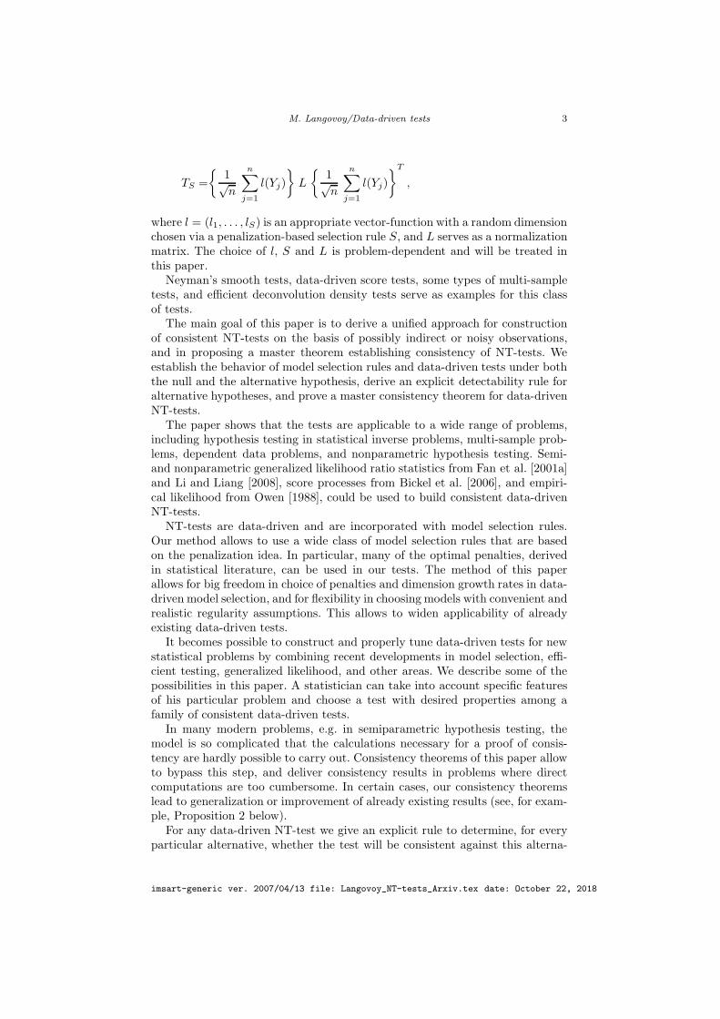
We introduce a class of data-driven statistical NT-tests. These tests are con-cerned with testing hypotheses about variables of interestX1, X2, . . . , Xm on thebasis of auxiliary third-party variables Y1, Y2, . . . , Yn, and their correspondingtest statistics are, in general, random quadratic forms of the type



TS =

{1√n

n∑

j=1

l(Yj)

}L

{1√n

n∑

j=1

l(Yj)

}T

,

where l = (l1, . . . , lS) is an appropriate vector-function with a random dimensionchosen via a penalization-based selection rule S, and L serves as a normalizationmatrix. The choice of l, S and L is problem-dependent and will be treated inthis paper.

Neyman’s smooth tests, data-driven score tests, some types of multi-sampletests, and efficient deconvolution density tests serve as examples for this classof tests.

The main goal of this paper is to derive a unified approach for constructionof consistent NT-tests on the basis of possibly indirect or noisy observations,and in proposing a master theorem establishing consistency of NT-tests. Weestablish the behavior of model selection rules and data-driven tests under boththe null and the alternative hypothesis, derive an explicit detectability rule foralternative hypotheses, and prove a master consistency theorem for data-drivenNT-tests.

The paper shows that the tests are applicable to a wide range of problems,including hypothesis testing in statistical inverse problems, multi-sample prob-lems, dependent data problems, and nonparametric hypothesis testing. Semi-and nonparametric generalized likelihood ratio statistics from Fan et al. [2001a]and Li and Liang [2008], score processes from Bickel et al. [2006], and empiri-cal likelihood from Owen [1988], could be used to build consistent data-drivenNT-tests.

NT-tests are data-driven and are incorporated with model selection rules.Our method allows to use a wide class of model selection rules that are basedon the penalization idea. In particular, many of the optimal penalties, derivedin statistical literature, can be used in our tests. The method of this paperallows for big freedom in choice of penalties and dimension growth rates in data-driven model selection, and for flexibility in choosing models with convenient andrealistic regularity assumptions. This allows to widen applicability of alreadyexisting data-driven tests.

It becomes possible to construct and properly tune data-driven tests for newstatistical problems by combining recent developments in model selection, effi-cient testing, generalized likelihood, and other areas. We describe some of thepossibilities in this paper. A statistician can take into account specific featuresof his particular problem and choose a test with desired properties among afamily of consistent data-driven tests.

In many modern problems, e.g. in semiparametric hypothesis testing, themodel is so complicated that the calculations necessary for a proof of consis-tency are hardly possible to carry out. Consistency theorems of this paper allowto bypass this step, and deliver consistency results in problems where directcomputations are too cumbersome. In certain cases, our consistency theoremslead to generalization or improvement of already existing results (see, for exam-ple, Proposition 2 below).

For any data-driven NT-test we give an explicit rule to determine, for everyparticular alternative, whether the test will be consistent against this alterna-



tive. This rule allows us to describe, in a closed form, the set of detectablealternatives for every NT-test.

1.2. Paper outline

In Section 2, we describe the framework and introduce a class of NT-statistics,for the case of deterministic model dimension. This is one of the main buildingblocks for our tests. In Section 3, we define penalization-based model selectionrules that will be used in our tests, and introduce a concept of data-driven tests.In Section 4, we establish behavior of model selection rules and data-driven NT-tests for the case when the alternative hypothesis is true. In this Section, wealso derive an explicit consistency condition that allows to check whether anyparticular alternative could be detected by the data-driven NT-test. In Section 5we describe what happens with a data-driven NT-test under the null hypothesis.Finally, in Section 6 a master consistency theorem for data-driven NT-tests isgiven. Additionally, each section contains examples illustrating the applicabilityof new concepts by connecting them to a variety of well-established special cases.

2. NT-statistics

2.1. Basic definition: NT-statistics with deterministic dimensions

Let X1, X2, . . . be a sequence of random variables with values in an arbitrarymeasurable space X. Suppose that for everym the random variablesX1, . . . , Xm

have the joint distribution Pm from the family of distributions Pm. Supposethere is a given functional F acting from the direct product of the families⊗∞

m=1 Pm = (P1,P2, . . .) to a known set Θ, and that F(P1, P2, . . .) = θ. Weconsider the following generic

Problem: test the hypothesis H0 : θ ∈ Θ0 ⊂ Θ against the alternativeHA : θ ∈ Θ1 = Θ\Θ0, on the basis of indirect observations Y1, . . . , Yn havingtheir values in an arbitrary measurable space Y (i.e. not necessarily on the basisof variables of interest X1, . . . , Xm).

Here Θ can be any set, for example, a functional space; correspondingly,parameter θ can be infinite dimensional. It is not assumed that Y1, . . . , Yn

are independent or identically distributed. The measurable space Y can be in-finite dimensional. This allows to apply the results of this paper in statisticsfor stochastic processes. Additional assumptions on Y ′

i s will be imposed below,when it would be necessary.

An important feature of our approach is that we are able to consider the casewhen the null hypothesis H0 is not about observable Y ′

i s, but about some otherrandom variables X1, . . . , Xm. This makes it possible to use our method in thecase of statistical inverse problems (see Langovoy [2008], and Examples 2 and3 below). Under conditions of Theorem 3 of the present paper, it would be stillpossible to extract from Y ′

i s enough information in order to build a consistenttest about X ′

is.Now we introduce one of the main concepts of this paper.



Definition 1. (NT-statistics with deterministic dimensions). Supposewe have n random observations Y1, . . . , Yn with values in a measurable spaceY. Let k be a fixed number and l = (l1, . . . , lk) be a vector-function, whereli : Y → R for i = 1, . . . , k are some known Lebesgue measurable functions. Set

L = {E0[l(Y )]Tl(Y )}−1

, (1)

where the mathematical expectation E0 is taken with respect to P0, and P0

is the (fixed and known in advance) distribution function of some auxilliaryrandom variable Y, where Y is assuming its values in the space Y. Assume thatE0 l(Y ) = 0 and L is well defined in the sense that all its elements are finite.Put

Tk =

{1√n

n∑

j=1

l(Yj)

}L

{1√n

n∑

j=1

l(Yj)

}T

. (2)

We call Tk a statistic of Neyman’s type (or NT-statistic).

Here l1, . . . , lk can be some score functions, as was the case for the classicalNeyman’s test Neyman [1937], but it is possible to use any other functions,depending on the problem under consideration. We prove below that underadditional assumptions it is possible to construct consistent tests of such formwithout using scores in (2). We will discuss different possible sets of meaningfuladditional assumptions on l1, . . . , lk in Sections 4 - 6.

Scores are based on the notion of maximum likelihood. In our constructionsit is possible to use, for example, truncated, penalized or generalized likelihoodto build a test. It is even possible to use functions l1, . . . , lk such that they areunrelated to any kind of likelihood.

If, for example, Y ′i s are equally distributed, then the natural choice for P0 is

their distribution function under the null hypothesis. Thus, L will be the inverseto the covariance matrix of the vector l(Y ). Such construction is often used inscore tests for simple hypothesis. But our definition allows to use a reasonablesubstitution instead of the covariance matrix. This is helpful for testing in cer-tain semi- or nonparametric models.

2.2. Examples of NT-tests

Example 1. Neyman’s smooth tests. The basic example of an NT-statisticis the Neyman’s smooth test statistic for simple hypotheses (see Neyman [1937]).Let X1, . . . , Xn be i.i.d. random variables. Consider the problem of testing thesimple null hypothesis H0 that the X ′

is have the uniform distribution on [0, 1].Let {φj} denote the family of orthonormal Legendre polynomials on [0, 1]. Thenfor every k one has the test statistic

Tk =

k∑

j=1

{1√n

n∑

i=1

φj(Xi)

}2

.



We see that Neyman’s classical test statistic is an NT-statistic, with Yi = Xi

for all i in this very simplest example.

Hypothesis testing in statistical inverse problems is an important but still arather unexplored area in modern statistics. Applications to statistical inverseproblems served as the main motivation for studying NT-tests.

Example 2. Statistical inverse problems. The most well-known examplehere is the deconvolution problem. This problem appears when one has noisysignals or measurements: in physics, seismology, optics and imaging, engineer-ing. It is a building block for many complicated statistical inverse problems.The book Carroll et al. [2006] provides many examples related to deconvolutionproblems. In Langovoy [2008], data-driven score tests for the problem were con-structed, thus solving the deconvolution density testing problem. The solutionof Langovoy [2008] is a special case of the results of the present paper.

The basic deconvolution density testing problem is formulated as follows.Suppose that instead of Xi one observes Yi, where

Yi = Xi + εi,

and ε′is are i.i.d. with a known density h with respect to the Lebesgue measure λ;also Xi and εi are independent for each i and E εi = 0, 0 < E ε2 < ∞. Assumethat X has a density with respect to λ. Our null hypothesis H0 is the simplehypothesis that X has a known density f0 with respect to λ. Let us choose forevery k ≤ d(n) an auxiliary parametric family {fθ}, θ ∈ Θ ⊆ R

k such thatf0 from this family coincides with f0 from the null hypothesis H0. The true Fpossibly has no relation to the chosen {fθ}. Set

l(y) =

∂∂θ

( ∫Rfθ(s)h( y − s) ds

)∣∣∣θ=0∫

Rf0(s)h( y − s) ds

(3)

and define the corresponding test statistic Uk by the formula (2). Under ap-propriate regularity assumptions, Uk is an NT-statistic (see Langovoy [2007]).As was shown in Langovoy [2008], the data-driven test US , based on Uk, isasymptotically consistent against a wide class of nonparametric alternatives.

Subsequently, Butucea et al. [2009] proposed an adaptive goodness-of-fit testfor this model with indirect observations, which appears to be the first nonpara-metric adaptive test in statistical inverse problems. The test from Butucea et al.[2009] is restricted to polynomially smooth error density and to signal densitiescoming from even narrower smoothness classes. The data-driven test US fromLangovoy [2007] was intended to cover wider scope of applications and to havea flexible penalization procedure, so optimality properties were not attainableover the intended consistency range. Adaptive modifications of US can be con-structed via using special penalties, tailored to deliver minimax optimality forconvolution densities from properly restricted classes (analogously to the methodof Fan et al. [2001b]).

The following example serves as an illustration of applicability of NT-teststo multisample problems.



Example 3. Rank Tests for Independence. Let X1 = (V1,W1), . . . , Xn =(Vn,Wn) be i.i.d. random variables with the distribution function D and themarginal distribution functions F and G for V1 and W1. Assume that F andG are continuous, but unknown. It is the aim to test the null hypothesis ofindependence

H0 : D(v, w) = F (v)G(w), v, w ∈ R, (4)

against a wide class of alternatives. The following construction was proposed inKallenberg and Ledwina [1999].Let φj denote the j−th orthonormal Legendre polynomial (i.e., φ1(x) =

√3(2x−

1), φ2(x) =√5(6x2−6x+1), etc.). The score test statistic from Kallenberg and Ledwina

[1999] is

Tk =

k∑

j=1

{1√n

n∑

i=1

φj

(Ri − 1/2

n

)φj

(Si − 1/2

n

)}2

, (5)

where Ri stands for the rank of Vi among V1, . . . , Vn and Si for the rank of Wi

among W1, . . . ,Wn. Thus defined Tk satisfies Definition 1 of NT-statistics: put

Yi = (Y(1)i , Y

(2)i ) :=

(Ri − 1/2

n,Si − 1/2

n

)

and lj(Yi) := φj(Y(1)i )φj(Y

(2)i ). Under the null hypothesis Lk = Ek×k, and

E0l(Z) = 0. Thus, Tk is an NT-statistic. New Yi depends on the original X ′is

(= (Vi,Wi)′s) in a nontrivial way, but still contains some information about the

pair of interest. �Many other examples, including data-driven tests based on partial likelihood

(see Cox [1975]), can be found in Langovoy [2007] and Langovoy [2009].

3. Data-driven tests and model selection

3.1. Selection rules and data-driven tests: definitions

It was shown that for achieving optimality of efficient score tests it is im-portant to select the right number of components in the test statistic (seeBickel and Ritov [1992], Eubank et al. [1993], Fan [1996], Kallenberg [2002]).Therefore, we provide a corresponding refinement for NT-statistics as well. Us-ing the idea of a penalized likelihood, we propose a general mathematical frame-work for constructing rules to find reasonable model dimensions. We make ourtests data-driven, i.e., the tests choose a reasonable number of components inthe test statistics automatically and accordingly to the data. Our constructionoffers substantial freedom in the choice of penalties and possible basis models.This way, it is easy to take into account specific features of particular problemsand to choose suitable statistical models and reasonable penalties in order tobuild tests with desired properties for each particular problem.

We will not restrict a possible number of components in test statistics bysome fixed number, but instead we allow the number of components to grow



unlimitedly as the number of observations grows. This is important because themore observations Y1, . . . , Yn we have, the more information is available aboutthe problem. This makes it possible to give a more detailed description of thephenomena under investigation. In our case this means that the complexity ofthe model and the possible number of components in the corresponding teststatistic grow with n at a controlled rate.

Denote by Mk a statistical model designed for a specific statistical problemsatisfying assumptions of Section 2. Assume that the true parameter value θbelongs to the parameter set of Mk, call it Θk. We say that the family ofmodels Mk for k = 1, 2, . . . is nested if for their parameter sets it holds thatΘ1 ⊆ Θ2 ⊆ . . . . Here Θ′

ks can be infinite-dimensional. We also do not requirethat all Θ′

ks are different (analogously to Birge and Massart [2001], p. 221).Let Tk be an arbitrary statistic for testing validity of the model Mk on the basisof observations Y1, . . . , Yn. The following definition applies for the sequence ofstatistics {Tk}.Definition 2. (Penalty, selection rule, and data-driven tests) Considera nested family of models Mk for k = 1, . . . , d(n), where d(n) is a controlsequence, giving the largest possible model dimension for the case of n obser-vations. Choose a function π(·, ·) : N × N → R, where N is the set of natu-ral numbers. Assume that π(1, n) < π(2, n) < . . . < π(d(n), n) for all n andπ(j, n)−π(1, n) → ∞ as n → ∞ for every j = 2, . . . , d(n). Call π(j, n) a penaltyattributed to the j-th model Mj and the sample size n.

Then a selection rule S for the sequence of statistics {Tk} is an integer-valuedrandom variable satisfying the condition

S = min{k : 1 ≤ k ≤ d(n); Tk−π(k, n) ≥ Tj−π(j, n), j = 1, . . . , d(n)

}. (6)

We call TS a data-driven test statistic for testing validity of the initial model.

The definition is expected to be applied, of course, only if the sequence {Tk}is increasing unboundedly, in the sense that Tk(Y1, . . . , Yn) → ∞ in probabilityas k → ∞.

In statistical literature, one often tries to choose penalties such that theypossess some sort of minimax or Bayesian optimality. Classical examples of thepenalties constructed via this approach are Schwarz’s penalty π(j, n) = j logn(see Schwarz [1978]), and minimum description length penalties, see Rissanen[1983]. For more examples of optimal penalties and recent developments, seeAbramovich et al. [2007], Birge and Massart [2001] or Bunea et al. [2007]. Inthis paper, we do not aim for optimality of the penalization; our goal is to beable to build consistent data-driven tests based on different choices of penalties.The penalization technique that we use in this paper allows for many possiblechoices of penalties. In our framework it is possible to use most of the penaltiesfrom the abovementioned papers. As an illustration, see Example 4 below.

3.2. Model selection rules: examples

Example 2, continued. Data-driven tests for inverse problems. Onecan incorporate Uk with the following selection rule widely used in statistical



literature:

S = min{k : 1 ≤ k ≤ d(n); Tk−k logn ≥ Tj−j logn, j = 1, 2, . . . , d(n)

}. (7)

This selection rule satisfies Definition 2, so thus defined US extends the teststatistic from Langovoy [2008] and makes it a data-driven NT-statistic. �

Example 4. Gaussian model selection.Birge and Massart in Birge and Massart[2001] proposed a method of model selection in a framework of Gaussian lin-ear processes. This framework is quite general and includes as special cases aGaussian regression with fixed design, Gaussian sequences and the model ofIbragimov and Has’minskii. In this example we briefly describe the construction(for more details see the original paper) and then discuss the relation with ourresults.

Given a linear subspace S of some Hilbert space H, we call Gaussian linearprocess on S, with mean s ∈ H and variance ε2, any process Y indexed by S ofthe form

Y (t) = 〈s, t〉+ εZ(t),

for all t ∈ S, and where Z denotes a linear isonormal process indexed by S

(i.e. Z is a centered and linear Gaussian process with covariance structureE[Z(t)Z(u)] = 〈t, u〉). Birge and Massart considered estimation of s in thismodel.Let S be a finite dimensional subspace of S and set γ(t) = ‖t‖2 − 2Y (t). Onedefines the projection estimator on S to be the minimizer of γ(t) with respectto t ∈ S. Given a finite or countable family {Sm}m∈M of finite dimensionallinear subspaces of S, the corresponding family of projection estimators sm,built for the same realization of the process Y, and given a nonnegative functionpen defined on M, Birge and Massart estimated s by a penalized projectionestimator s = sm, where m is any minimizer with respect to m ∈ M of thepenalized criterion

crit(m) = −‖sm‖2 + pen(m) = γ(sm) + pen(m).

They proposed some specific penalties pen such that the penalized projectionestimator has the optimal order risk with respect to a wide class of loss functions.The method of model selection of this paper has a relation with the one ofBirge and Massart [2001].

4. Data-driven NT-tests: alternative hypothesis case

In this section we study the behavior of NT-statistics and model selection rulesunder alternatives.

4.1. Explicit consistency condition

Let P denote the alternative distribution of Y ′i s. Suppose that EP l(Y ) exists.

Now we formulate the following crucial explicit consistency condition:



Consistency condition

〈C〉 there exists integer K = K(P ) ≥ 1 such thatEP l1(Y ) = 0, . . . , EP lK−1(Y ) = 0, EP lK(Y ) = CP 6= 0 ,

where l1, . . . , lk are as in Definition 1.

Example 1 (continued). Consistent smooth tests. In this basic problem,condition 〈C〉 is simply equivalent to the following one: there exists K = KP

such that EP φK(X) 6= 0. �

Example 2 (continued). Consistent density testing in inverse prob-lems. Let F be a true distribution of X . Here F is not supposed to be para-metric and possibly does not have a density. Let l be the score vector given by(3) and h be the known error density. As was shown in Langovoy [2008] andLangovoy [2007], if there exists an integer K = K(F ) ≥ 1 such that

EF∗h l1(Y ) = 0, . . . , EF∗h lK−1(Y ) = 0, EF∗h lK(Y ) 6= 0 , (8)

then US is asymptotically consistent against a wide class of nonparametric al-ternatives. �

We see that conditions equivalent to 〈C〉 naturally appear in studies of con-sistency of data-driven score tests. This condition explicitly describes whichdirections of alternatives to the null hypothesis can be captured by an NT-test.

4.2. Model selection under alternatives

We impose now two additional assumptions on the abstract model of Section2. First, we assume that Y1, Y2, . . . are identically distributed. We do not as-sume that Y1, Y2, . . . are independent. It is possible that the sequence of interestX1, X2, . . . consists of dependent and nonidentically distributed random vari-ables.

It is only important that the new (possibly obtained by a complicated trans-formation) sequence Y1, Y2, . . . obeys the consistency conditions. Then it is pos-sible to build consistent tests of hypotheses about X ′

is. The intuition behindthis is that, even after a complicated transformation, the transformed sequencestill can contain some part of the information about the sequence of interest.However, if the transformed sequence Y1, Y2, . . . is not chosen reasonably, thentest can be meaningless: it can be formally consistent, but against an empty oralmost empty set of alternatives.

Another assumption we impose is that the first K components of l(Yi)′s sat-

isfy both the law of large numbers and the multivariate central limit theorem, i.e.that for the vectors l(Y1) = (l1(Y1), . . . , lK(Y1)), . . . , l(Yn) = (l1(Yn), . . . , lK(Yn))it holds that

1

n

n∑

j=1

l(Yj) → EP l(Y ) in P − probability as n → ∞,



n−1/2n∑

j=1

(l(Yj)− EP l(Y )) →d N (9)

where N stands for a K−dimensional normal distribution with zero mean vec-tor.These assumptions restrict the choice of the function l and leave us with auniquely determined P0. Nonetheless, random variables of interest X1, . . . , Xn

are still allowed to be nonidentically distributed, and their transformed coun-terparts Y1, . . . , Yn are still allowed to be dependent.Without loss of generality, below we always assume that

limn→∞

d(n) = ∞ . (10)

The (relatively degenerate) case when d(n) is nondecreasing and bounded fromabove by some constant D can be handled analogously to the method of thispaper, see Langovoy [2007].

To clarify the statement of the next theorem, we remind that in Definition 1L is a k × k−matrix. Below we will sometimes denote it Lk in order to stressthe model dimension. Accordingly, ordered eigenvalues of Lk will be denoted

λ(k)1 ≥ λ

(k)2 ≥ . . . ≥ λ

(k)k . We have the sequence of matrices {Lk}∞k=1 and each

matrix has its own eigenvalues. Whenever possible, we will use the simplifiednotation from Definition 1.

Proposition 1. Let 〈C〉 and (10) holds and

limn→∞

supk≤d(n)

π(k, n)

nλ(k)k

= 0 . (11)

Then

limn→∞

P (S ≥ K) = 1 .

Remark 1. Condition (11) means that not only n tends to infinity, but that it isalso possible for k to grow infinitely, but at the controlled rate. This conditionis needed to ensure that the penalty π is not so large that it trivializes the data-driven model choice. It is easy to check (11) for any specific function π since theeigenvalues of Lk are known in advance, and it is easy to satisfy (11) becausewe are free to choose π from the whole range of possible penalty functions.

4.3. Data-driven NT-tests under detectable alternatives

Now suppose that the alternative distribution P is such that 〈C〉 is satisfied andthat there exists a sequence {rn}∞n=1 such that limn→∞ rn = ∞ and

〈A〉 P

(1

n

∣∣∣∣n∑

i=1

[lK(Yi)− EP lK(Yi)

]∣∣∣∣ ≥ y

)= O

(1

rn

).



Note that in 〈A〉 we do not require uniformity in y, i.e. rn gives us the rate, butthe exact bound can depend on y. In some sense condition 〈A〉 is a way to makethe weak law of large numbers for lK(Yi)

′s more precise. The following lemmashows that condition 〈A〉 is often easily satisfied.

Lemma 1. Let lK(Yi)′s be bounded i.i.d. random variables with finite expecta-

tion and variance σ2. Then condition 〈A〉 is satisfied with rn = exp(ny2/2σ).

Therefore, one can often expect exponential rates in 〈A〉, but even a much slowerrate is not a problem. The proof of this standard lemma is omitted.

The main result of this section is the following theorem that describes asymp-totic behavior of NT-tests under alternative hypotheses.

Theorem 1. Let 〈A〉, 〈C〉, (10) and (11) holds and

d(n) = o(rn) as n → ∞ . (12)

Then TS →P ∞ as n → ∞ .

Remark 2. Sometimes it is possible to find asymptotic distributions of NT-statistics, both under the null hypothesis and under alternatives. In order todo this, one can approximate the quadratic form Tk by certain quadratic formin N1, . . . , Nk, where Ni’s are Gaussian random variable with suitably chosenmean and covariance structure. When this approximation is possible, the errorof approximation is often of order n−1/2 and depends on the smallest eigenvalueof the covariance of l(Y1). See Gotze and Tikhomirov [1999], p. 1078 for moredetails.

Note that for proving consistency of data-driven NT-tests one doesn’t need toknow asymptotic distributions of underlying NT-statistics. Theorem 1 is strongenough for our purposes.

5. Data-driven NT-tests under the null hypothesis

Now we study the asymptotic behavior of data-driven NT-statistics under thenull hypothesis.

5.1. Proper penalties and majorants for data-driven tests

The following two technical definitions are useful for data-driven model selectionin general.

Definition 3. (Penalties of proper weight). Let {Tk} be a sequence of NT-statistics and S be a selection rule for it. Suppose that λ1 ≥ λ2 ≥ . . . are orderedeigenvalues of L, where L is defined by (1). We say that the penalty π(k, n) inS is of proper weight, if the following conditions holds:

1. there exists sequences of real numbers {s(k, n)}∞k,n=1 , {t(k, n)}∞

k,n=1 , suchthat

(a)

limn→∞

supk≤un

s(k, n)

nλ(k)k

= 0 ,



where {un}∞n=1 is some real sequence such that limn→∞ un = ∞.

(b) limn→∞ t(k, n) = ∞ for every k ≥ 2,

limk→∞ t(k, n) = ∞ for every fixed n.

2. s(k, n) ≤ π(k, n)− π(1, n) ≤ t(k, n) for all k, n.3.

limn→∞

supk≤mn

π(k, n)

nλ(k)k

= 0 ,

where {mn}∞n=1 is some real sequence such that limn→∞ mn = ∞.

Definition 3 is more general than required for our present goals. As can be seenfrom Theorem 2 below, in our research on consistency of data-driven tests wecan assume un = mn = d(n) for all n, where d(n) is the model complexitygrowth rate from Definition 2. We have chosen to state Definition 3 in its fullgenerality because of its general usefulness in model selection.

Condition 2 of Definition 3 is needed to ensure that the penalty π actuallypenalizes models with large dimension k. The choice of s(k, n) and t(k, n) willbe explained below.For notational convenience, for l = (l1, . . . , lk) from Definition 1 we denote

lj :=1

n

n∑

i=1

lj(Yi) , l := (l1, l2, . . . , lk) (13)

and define a quadratic form

Qk(l) = (l1, l2, . . . , lk)L (l1, l2, . . . , lk)T. (14)

In the new notation, Tk = Qk(l), where Tk is the statistic from Definition 1.Below we also use the notation of Definition 3.

Definition 4. (Proper majorant). Let S be with a penalty of proper weight.Assume that there exists a Lebesgue measurable function ϕ(·, ·) : R × R → R,such that ϕ is monotonically decreasing in the second argument and monotoni-cally nondecreasing in the first one, and assume that

1. for every ε > 0 there exists K = Kε such that for every n > n(ε)

〈B1〉un∑

k=Kε

ϕ(k; s(k, n)) < ε ,

where {un}∞n=1 is as in Definition 3.2.

〈B2〉 P0 (nQk(l) ≥ y) ≤ ϕ(k; y)

for all k ≥ 1 and y ∈ [s(k, n); t(k, n)] , where P0 is as in Definition 1.

We call ϕ a proper majorant for (large deviations of) the statistic TS . Equiva-lently, we say that (large deviations of) the statistic TS are properly majoratedby ϕ.



Again, one is free to assume in this Definition that un = d(n) for all n. In Def-initions 3 and 4 we need some lower bound s(k, n) to be sure that the penaltyπ is not ”too light”, i.e. that the penalty somehow affects the choice of themodel dimension and protects us from choosing a ”too complicated” model. Innontrivial cases, it follows from 〈B1〉 that s(k, n) → ∞ as k → ∞. The exactchoice of functions s and t for each specific problem is dictated by the variantof inequalities 〈B1〉 and 〈B2〉 that holds in this particular statistical problem.

Example 1 (continued). Model selection for data-driven smooth tests.Put π(k, n) = k logn. Then Prohorov’s inequality (see Appendix) suggests thefollowing possible ϕ in Definition 4:

ϕ(k; y) =150210

Γ(k/2)

(y2

2

) k−1

2

exp

{− y2

4

}, (15)

with, for example, s(k, n) := 3k and t(k, n) := 1/4√

n/k . All conditions ofDefinitions 3 and 4 can be easily checked. It follows that one can afford any

model dimension growth rate such that d(n) = o({n/ logn}1/3). �For many test statistics Prohorov’s inequality can’t be used to estimate the

large deviations. This is usually the case for more complicated models wherethe matrix L is not diagonal. This is typical for statistical inverse problems aswell as for problems with dependent data. If one deals with likelihood-basedNT-statistics, then the easiest way is to use large deviations results that wereestablished in studies on usual likelihood tests and their efficiencies. Otherwise,one has to find a direct way to estimate the test statistic.

Remark 3. There is a general approach that makes it possible to check conditionsof Definition 4, and to study distributions of NT-statistics for moderate samplesizes, in many particular situations. This method consists of two steps. On thefirst step, one approximates the quadratic formQ(l(Y )) by the simpler quadraticform Q(N), where N is the Gaussian random variable with the same mean andcovariance structure as l(Y ). This approximation is possible, for example, underconditions given in Gotze and Tikhomirov [1999] or Bentkus and Gotze [1996].These authors gave the rate of convergence for such approximation. The secondstep is to establish a large deviation result for the quadratic form Q(N); thisform has a more predictable distribution. Even for strongly dependent randomvariables, one can hope to use results from Horvath and Shao [1999].

5.2. Data-driven NT-statistics under null hypotheses

The following is the key result describing the behaviour of a data-driven NT-statistic under the null hypothesis.

Theorem 2. Let {Tk} be a sequence of NT-statistics and S be a selection rulefor the sequence. Assume that the penalty in S is of proper weight and that largedeviations of statistics TS are properly majorated. Suppose that

d(n) ≤ min{un ,mn} . (16)

Then S = OP0(1) and TS = OP0

(1).



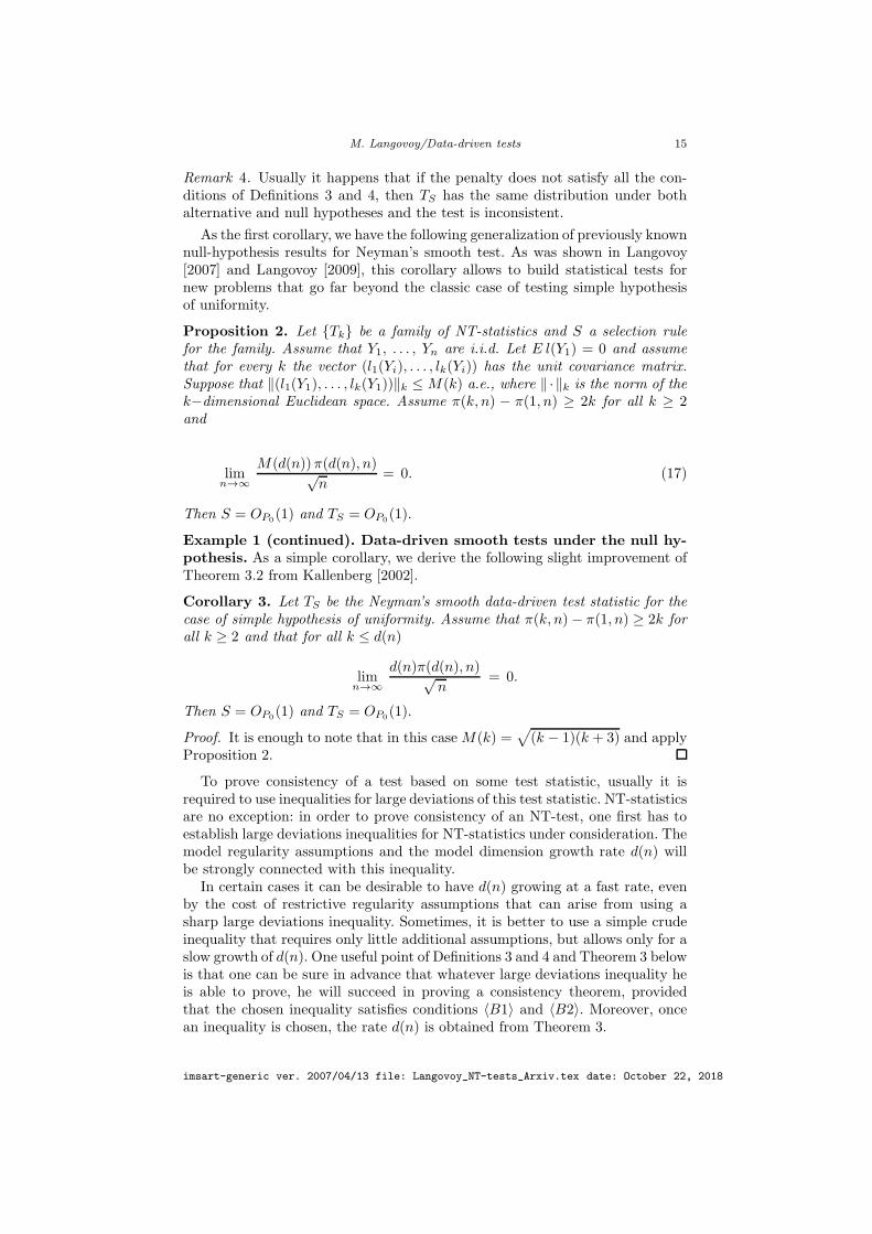
Remark 4. Usually it happens that if the penalty does not satisfy all the con-ditions of Definitions 3 and 4, then TS has the same distribution under bothalternative and null hypotheses and the test is inconsistent.

As the first corollary, we have the following generalization of previously knownnull-hypothesis results for Neyman’s smooth test. As was shown in Langovoy[2007] and Langovoy [2009], this corollary allows to build statistical tests fornew problems that go far beyond the classic case of testing simple hypothesisof uniformity.

Proposition 2. Let {Tk} be a family of NT-statistics and S a selection rulefor the family. Assume that Y1, . . . , Yn are i.i.d. Let E l(Y1) = 0 and assumethat for every k the vector (l1(Yi), . . . , lk(Yi)) has the unit covariance matrix.Suppose that ‖(l1(Y1), . . . , lk(Y1))‖k ≤ M(k) a.e., where ‖ ·‖k is the norm of thek−dimensional Euclidean space. Assume π(k, n) − π(1, n) ≥ 2k for all k ≥ 2and

limn→∞

M(d(n))π(d(n), n)√n

= 0. (17)


(1).

Example 1 (continued). Data-driven smooth tests under the null hy-pothesis. As a simple corollary, we derive the following slight improvement ofTheorem 3.2 from Kallenberg [2002].

Corollary 3. Let TS be the Neyman’s smooth data-driven test statistic for thecase of simple hypothesis of uniformity. Assume that π(k, n)− π(1, n) ≥ 2k forall k ≥ 2 and that for all k ≤ d(n)

limn→∞

d(n)π(d(n), n)√n

= 0.


(1).

Proof. It is enough to note that in this case M(k) =√(k − 1)(k + 3) and apply

Proposition 2.

To prove consistency of a test based on some test statistic, usually it isrequired to use inequalities for large deviations of this test statistic. NT-statisticsare no exception: in order to prove consistency of an NT-test, one first has toestablish large deviations inequalities for NT-statistics under consideration. Themodel regularity assumptions and the model dimension growth rate d(n) willbe strongly connected with this inequality.

In certain cases it can be desirable to have d(n) growing at a fast rate, evenby the cost of restrictive regularity assumptions that can arise from using asharp large deviations inequality. Sometimes, it is better to use a simple crudeinequality that requires only little additional assumptions, but allows only for aslow growth of d(n).One useful point of Definitions 3 and 4 and Theorem 3 belowis that one can be sure in advance that whatever large deviations inequality heis able to prove, he will succeed in proving a consistency theorem, providedthat the chosen inequality satisfies conditions 〈B1〉 and 〈B2〉. Moreover, oncean inequality is chosen, the rate d(n) is obtained from Theorem 3.



6. Consistency theorem

Now we formulate the general consistency theorem for data-driven NT-tests. Weunderstand consistency of the test based on TS in the sense that under the nullhypothesis TS is bounded in probability, while under fixed alternatives TS → ∞in probability.

Theorem 3. (Consistency of data-driven NT-tests.) Let {Tk} be a se-quence of NT-statistics and S be a selection rule for it. Assume that the penaltyin S is of proper weight. Assume that conditions (A), (10) and (11) are satis-fied and that d(n) = o(rn), d(n) ≤ min{un,mn}. Then the test based on TS isconsistent against any alternative distribution P satisfying condition (C).

Without a general consistency theorem, one has to perform the whole proofof consistency of a data-driven test anew for every particular problem. This be-comes especially difficult in many semi- and nonparametric problems. Using thegeneral consistency Theorem 3, some type of consistency result can be obtainedfor any data-driven NT-statistics, and types of detectable alternatives can becharacterized explicitly.

Example 4 (continued). Data-driven tests for Gaussian linear pro-cesses. In the model of Birge and Massart γ(t) is the least squares criterionand sm is the least squares estimator of s, which is in this case the maximumlikelihood estimator. Therefore ‖sm‖2 is the Neyman score for testing the hy-pothesis s = 0 within this model. Risk-optimizing penalties pen proposed inBirge and Massart [2001] satisfy the conditions of Definition 2 (after the changeof notations pen(m) = π(m,n); for the explicit expressions of pen′s see theoriginal paper). Therefore, ‖sm‖2 is, in our terminology, the data-driven NT-statistic. As follows from the consistency Theorem 3, ‖sm‖2 can be used fortesting s = 0 and has a good range of consistency, even though this particularpenalty probably does not lead to adaptively optimal testing, see Baraud et al.[2003]. �

Many other examples of applications of the consistency theorem can be foundin Langovoy [2007] and Langovoy [2009].

Remark 5. In general, it seems to be possible to use the idea of a score pro-cess and some other technics from Bickel et al. [2006] in order to construct andanalyze NT-statistics. This can be seen by the fact that such applications asin Example 6 naturally appear in both papers. The difference with the abovepaper would be that we prefer to use test statistics of the form (2) rather thanintegrals or suprema of score processes.

In semi- and nonparametric models, generalized likelihood ratios from Fan et al.[2001a] and Li and Liang [2008], as well as different modifications of empiricallikelihood, could also be a powerful tool for constructing NT-statistics.

Acknowledgments. Author would like to thank Fadoua Balabdaoui, ShotaGugushvili and Axel Munk for helpful discussions. Most of this research wasdone at Georg-August-University of Gottingen, Germany.



References

A. N. Kolmogorov. Sulla Determinazione Empirica di una Legge di Dis-tribuzione. Giornale dell’Istituto Italiano degli Attuari, 4:83–91, 1933.

Holger Dette. A consistent test for heteroscedasticity in nonparametric regres-sion based on the kernel method. Journal of statistical planning and inference,103(1):311–329, 2002.

Dino Sejdinovic, Bharath Sriperumbudur, Arthur Gretton, and Kenji Fukumizu.Equivalence of distance-based and rkhs-based statistics in hypothesis testing.The Annals of Statistics, pages 2263–2291, 2013.

Wojciech Zaremba, Arthur Gretton, and Matthew Blaschko. B-test: A non-parametric, low variance kernel two-sample test. In Advances in neural infor-mation processing systems, pages 755–763, 2013.

Kacper Chwialkowski, Heiko Strathmann, and Arthur Gretton. A kernel testof goodness of fit. In International Conference on Machine Learning, pages2606–2615, 2016.

Ya. Nikitin. Asymptotic efficiency of nonparametric tests. Cambridge UniversityPress, Cambridge, 1995. ISBN 0-521-47029-3.

J. Neyman. Smooth test for goodness of fit. Skand. Aktuarietidskr., 20:150–199,1937.

S.S. Wilks. The large-sample distribution of the likelihood ratio for testingcomposite hypotheses. Ann. Math. Stat., 9:60–62, 1938.

L. Le Cam. On the asymptotic theory of estimation and testing hypotheses.In Proceedings of the Third Berkeley Symposium on Mathematical Statisticsand Probability, 1954–1955, vol. I, pages 129–156, Berkeley and Los Angeles,1956. University of California Press.

J. Neyman. Optimal asymptotic tests of composite statistical hypotheses. InProbability and statistics: The Harald Cramer volume (edited by Ulf Grenan-der), pages 213–234. Almqvist & Wiksell, Stockholm, 1959.

P. J. Bickel and Y. Ritov. Testing for goodness of fit: a new approach. InNonparametric statistics and related topics (Ottawa, ON, 1991), pages 51–57.North-Holland, Amsterdam, 1992.

T. Inglot and T. Ledwina. Asymptotic optimality of data-driven Neyman’s testsfor uniformity. Ann. Statist., 24(5):1982–2019, 1996. ISSN 0090-5364.

J. Fan, C. Zhang, and J. Zhang. Generalized likelihood ratio statistics and Wilksphenomenon. Ann. Stat., 29(1):153–193, 2001a.

P. J. Bickel, Y. Ritov, and T. M. Stoker. Tailor-made tests for goodness offit to semiparametric hypotheses. Ann. Statist., 34(2):721–741, 2006. ISSN0090-5364.

Runze Li and Hua Liang. Variable selection in semiparametric regressionmodeling. Ann. Statist., 36(1):261–286, 2008. ISSN 0090-5364. . URLhttp://dx.doi.org/10.1214/009053607000000604.

P. J. Bickel, C. A. J. Klaassen, Y. Ritov, and J. A. Wellner. Efficient and adap-tive estimation for semiparametric models. Johns Hopkins Series in the Math-ematical Sciences. Johns Hopkins University Press, Baltimore, MD, 1993.ISBN 0-8018-4541-6.

I. A. Ibragimov and R. Z. Has′minskiı. Statistical estimation, volume 16 ofApplications of Mathematics. Springer-Verlag, New York, 1981. ISBN 0-387-90523-5. Asymptotic theory, Translated from the Russian by Samuel Kotz.

W. C. M. Kallenberg and T. Ledwina. Consistency and Monte Carlo simulation


http://dx.doi.org/10.1214/009053607000000604


of a data driven version of smooth goodness-of-fit tests. Ann. Statist., 23(5):1594–1608, 1995. ISSN 0090-5364.

Yu. I. Ingster. Asymptotically minimax hypothesis testing for nonparametricalternatives. I, II, III. Math. Methods Statist., 2:85–114, 171–189, 249–268,1993. ISSN 1066-5307.

V. G. Spokoiny. Adaptive hypothesis testing using wavelets. Ann. Statist., 24(6):2477–2498, 1996. ISSN 0090-5364.

M. Langovoy. Data-driven efficient score tests for deconvolution hy-potheses. Inverse Problems, 24(2):025028 (17pp), 2008. URLhttp://stacks.iop.org/0266-5611/24/025028.

Hajo Holzmann, Nicolai Bissantz, and Axel Munk. Density testing in a contam-inated sample. Journal of multivariate analysis, 98(1):57–75, 2007.

Nicolai Bissantz, Thorsten Hohage, Axel Munk, and Frits Ruymgaart. Conver-gence rates of general regularization methods for statistical inverse problemsand applications. SIAM Journal on Numerical Analysis, 45(6):2610–2636,2007.

A. B. Owen. Empirical likelihood ratio confidence intervals for a single func-tional. Biometrika, 75(2):237–249, 1988. ISSN 0006-3444.

R. J. Carroll, D. Ruppert, L. A. Stefanski, and C. M. Crainiceanu. Measure-ment error in nonlinear models, volume 105 of Monographs on Statistics andApplied Probability. Chapman & Hall/CRC, Boca Raton, FL, second edition,2006. ISBN 978-1-58488-633-4; 1-58488-633-1. A modern perspective.

M. Langovoy. Data-driven goodness-of-fit tests. University of Gottingen,Gottingen, 2007. Ph.D. thesis.

Cristina Butucea, Catherine Matias, Christophe Pouet, et al. Adaptivegoodness-of-fit testing from indirect observations. Ann. Inst. Henri PoincareProbab. Stat, 45(2):352–372, 2009.

J. Fan, C. Zhang, and J. Zhang. Generalized likelihood ratio statistics and Wilksphenomenon. Ann. Statist., 29(1):153–193, 2001b. ISSN 0090-5364.

W. C. M. Kallenberg and T. Ledwina. Data-driven rank tests for independence.J. Amer. Statist. Assoc., 94(445):285–301, 1999. ISSN 0162-1459.

D. R. Cox. Partial likelihood. Biometrika, 62(2):269–276, 1975. ISSN 0006-3444.M. Langovoy. Model selection, large deviations and consistency of data-driventests. EURANDOM Report No. 2009-007. EURANDOM, Eindhoven, 2009.

R. L. Eubank, J. D. Hart, and V. N. LaRiccia. Testing goodness of fit via non-parametric function estimation techniques. Comm. Statist. Theory Methods,22(12):3327–3354, 1993. ISSN 0361-0926.

J. Fan. Test of significance based on wavelet thresholding and Neyman’s trun-cation. J. Amer. Statist. Assoc., 91(434):674–688, 1996. ISSN 0162-1459.

W. C. M. Kallenberg. The penalty in data driven Neyman’s tests. Math. MethodsStatist., 11(3):323–340 (2003), 2002. ISSN 1066-5307.

L. Birge and P. Massart. Gaussian model selection. J. Eur. Math. Soc. (JEMS),3(3):203–268, 2001. ISSN 1435-9855.

G. Schwarz. Estimating the dimension of a model. Ann. Statist., 6(2):461–464,1978. ISSN 0090-5364.

J. Rissanen. A universal prior for integers and estimation by minimum descrip-tion length. Ann. Statist., 11(2):416–431, 1983. ISSN 0090-5364.

Felix Abramovich, Vadim Grinshtein, and Marianna Pensky. Onoptimality of Bayesian testimation in the normal means problem.Ann. Statist., 35(5):2261–2286, 2007. ISSN 0090-5364. . URL


http://stacks.iop.org/0266-5611/24/025028


http://dx.doi.org/10.1214/009053607000000226.Florentina Bunea, Alexandre B. Tsybakov, and Marten H. Wegkamp. Aggre-gation for Gaussian regression. Ann. Statist., 35(4):1674–1697, 2007. ISSN0090-5364. . URL http://dx.doi.org/10.1214/009053606000001587.

F. Gotze and A. N. Tikhomirov. Asymptotic distribution of quadratic forms.Ann. Probab., 27(2):1072–1098, 1999. ISSN 0091-1798.

V. Bentkus and F. Gotze. Optimal rates of convergence in the CLT for quadraticforms. Ann. Probab., 24(1):466–490, 1996. ISSN 0091-1798.

L. Horvath and Q.-M. Shao. Limit theorems for quadratic forms with applica-tions to Whittle’s estimate. Ann. Appl. Probab., 9(1):146–187, 1999. ISSN1050-5164.

Yannick Baraud, Sylvie Huet, and Beatrice Laurent. Adaptive tests of linearhypotheses by model selection. The Annals of Statistics, 31(1):225–251, 2003.

A. V. Prohorov. Sums of random vectors. Teor. Verojatnost. i Primenen., 18:193–195, 1973. ISSN 0040-361x.

Appendix.

Proof. (Proposition 1). By the law of large numbers, as n → ∞ ,

1

n

n∑

i=1

lK(Yi) →P CP 6= 0. (18)

We get

TK =

{1√n

n∑

i=1

−→l (Yi)

}Lk

{1√n

n∑

i=1

−→l (Yi)

}T

≥ λ(k)K

∥∥∥∥1√n

n∑

i=1

−→l (Yi)

∥∥∥∥2

≥ λ(k)K · 1

n

( n∑

i=1

lK(Yi)

)2

. (19)

By (18)

TK − π(K,n) ≥ nλ(k)K ·

( 1

n

n∑

i=1

lK(Yi))2− π(K,n)

= nλ(k)K

(C2

K + oP (1)CK

)− π(K,n)

= nλ(k)K C2

K + oP(nλ

(k)K

)− π(K,n) ,

and, because K and CK are constants determined by fixed P, condition (11)yields

TK − π(K,n) →P ∞ as n → ∞ . (20)

On the other hand, by (9)


http://dx.doi.org/10.1214/009053607000000226

http://dx.doi.org/10.1214/009053606000001587


(1√n

n∑

i=1

l1(Yi), . . . ,1√n

n∑

i=1

lK−1(Yi),

)→P N ,

where N is a (K − 1)−dimensional multivariate normal distribution with theexpectation vector equal to zero. This implies that Tk = OP (1) for all k =1, 2, . . . ,K − 1, because

Tk ≤ λ(k)1

∥∥∥∥1

n

n∑

i=1

l(Yi)

∥∥∥∥2

= λ(k)1 OP (1) = OP (1)

and λ(1)1 , λ

(2)1 , . . . , λ

(K−1)1 are constants and K < ∞. Now by (20)

limn→∞

K−1∑

k=1

P(Tk − π(k, n) ≥ TK − π(K,n)

)= 0 .

But for d(n) ≥ K

P (S < K) ≤K−1∑

k=1

P(Tk − π(k, n) ≥ TK − π(K,n)

),

and the theorem follows.

Because of assumption 〈A〉 we can prove the following lemma.

Lemma 2.

P

(∣∣∣∣1

n

n∑

i=1

lK(Yi)

∣∣∣∣ ≤√

x

λKn

)= O

(1

rn

).

Proof. Denote xn :=√

xλKn , and remember that by 〈C〉 we have EP lK(Yi) =

CK . Obviously, xn → 0 as n → ∞. We have

P

(∣∣∣∣1

n

n∑

i=1

lK(Yi)

∣∣∣∣ ≤ xn

)= P

(− xn ≤ 1

n

n∑

i=1

lK(Yi) ≤ xn

)

= P

(− xn − CK ≤ 1

n

n∑

i=1

(lK(Yi)− EP lK(Yi)

)≤ xn − CK

).

Here we get two cases. First, suppose CK > 0. Then we continue as follows:

P

(− xn − CK ≤ 1

n

n∑

i=1


)≤ xn − CK

)

≤ P

(1

n

n∑

i=1


)≤ xn − CK

)

≤ P

(∣∣∣∣1

n

n∑

i=1


)∣∣∣∣ ≥∣∣xn − CK

∣∣)

(for all n ≥ some nK)



≤ P

(∣∣∣∣1

n

n∑

i=1


)∣∣∣∣ ≥ CK

2

)= O

(1

rn

)

by 〈A〉, and so we proved the lemma for the case CK > 0. In case if CK < 0,we write

P

(− xn − CK ≤ 1

n

n∑

i=1


)≤ xn − CK

)

≤ P

(1

n

n∑

i=1


)≥ −xn − CK

)

and then we proceed analogously to the previous case.

Proof. (Theorem 1). Let x > 0. Since Tj > TK if j > K and (10) holds, we getby Proposition 1 that

P (TS ≤ x) =

d(n)∑

j=K

P (Tj ≤ x, S = j) + o(1)

≤ d(n)P (TK ≤ x) + o(1)

≤ d(n)P

(λK

1

n

( n∑

i=1

lK(Yi)

)2

≤ x

)+ o(1)

= d(n)P

(∣∣∣∣1

n

n∑

i=1

lK(Yi)

∣∣∣∣ ≤√

x

λKn

)+ o(1) .

Now by Lemma 2 and (12) we get

P (TS ≤ x) = O

(d(n)

rn

)+ o(1) = o(1) .

Proof. (Theorem 2). If S ≥ K, then Tk − T1 ≥ π(k, n) − π(1, n) for someK ≤ k ≤ d(n) and so, equivalently,

{1√n

n∑

i=1

l(Yi)

}L

{1√n

n∑

i=1

l(Yi)

}T

−{

1√n

n∑

i=1

l1(Yi)

}2

{E0[l1(Y )]T l1(Y )}−1 ≥ π(k, n)− π(1, n) (21)

for some K ≤ k ≤ d(n), where l = (l1, l2, . . . , lk). We can rewrite (21) in termsof the notation (13)-(14) as follows:

(√n l1, . . . ,

√n lk)L (

√n l1, . . . ,

√n lk)

T(22)



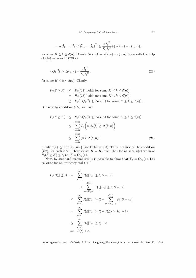
= n (l1, . . . , lk)L (l1, . . . , lk)T ≥ n l1

2

E0 l12+

(π(k, n)− π(1, n)

),

for some K ≤ k ≤ d(n). Denote ∆(k, n) := π(k, n)− π(1, n); then with the helpof (14) we rewrite (22) as

nQk(l) ≥ ∆(k, n) +n l1

2

E0 l12 , (23)

for some K ≤ k ≤ d(n). Clearly,

P0(S ≥ K) ≤ P0

((21) holds for some K ≤ k ≤ d(n)

)

= P0

((23) holds for some K ≤ k ≤ d(n)

)

≤ P0

(nQk(l) ≥ ∆(k, n) for some K ≤ k ≤ d(n)

).

But now by condition 〈B2〉 we have

P0(S ≥ K) ≤ P0

(nQk(l) ≥ ∆(k, n) for some K ≤ k ≤ d(n)

)

≤d(n)∑

k=K

P0

(nQk(l) ≥ ∆(k, n)

)

≤d(n)∑

k=K

ϕ(k; ∆(k, n)

), (24)

if only d(n) ≤ min{un,mn} (see Definition 3). Thus, because of the condition〈B2〉, for each ε > 0 there exists K = Kε such that for all n > n(ε) we haveP0(S ≥ K) ≤ ε, i.e. S = OP0

(1).Now, by standard inequalities, it is possible to show that TS = OP0

(1). Letus write for an arbitrary real t > 0

P0(|TS | ≥ t) =

Kε∑

m=1

P0(|Tm| ≥ t; S = m)

+

d(n)∑

m=Kε+1

P0(|Tm| ≥ t; S = m)

≤Kε∑

m=1

P0(|Tm| ≥ t) +

d(n)∑

m=Kε+1

P0(S = m)

=

Kε∑

m=1

P0(|Tm| ≥ t) + P0(S ≥ Kε + 1)

≤Kε∑

m=1

P0(|Tm| ≥ t) + ε

=: R(t) + ε.



For t → ∞ we have P0(|Tm| ≥ t) → 0 for every fixed m, so R(t) → 0 as t → ∞.Now it follows that for arbitrary ε > 0

limt→∞

P0(|TS | ≥ t) ≤ ε,

therefore

limt→∞

P0(|TS | ≥ t) = 0

and

limt→∞

P0(|TS | ≥ t) = 0.

This completes the proof.

Proof. (Theorem 3). Follows from Theorems 1 and 2 and our definition of con-sistency.

In the next proof we will need the following theorem from Prohorov [1973].

Theorem 4. Let Z1, . . . , Zn be i.i.d. random vectors with values in Rk. LetEZi = 0 and let the covariance matrix of Zi be equal to the identity matrix.Assume ‖Z1‖k ≤ L a.e. Then, for 2k ≤ y2 ≤ nL−2, we have

Pr

(‖n−1/2

n∑

i=1

Zi‖k ≥ y

)≤ 150210

Γ(k/2)

(y2

2

) k−1

2

exp

{− y2

2

(1− ηn

)},

where 0 ≤ ηn ≤ Lyn−1/2.

Proof. (Proposition 2) Here TS is an NT-statistic with Lk = Ek×k and λ(k)1 =

. . . = λ(k)k = 1. Therefore Theorem 2 is applicable. Put s(k, n) =

√2k , t(k, n) =

0.5√n M(k)−1. The Prohorov inequality is applicable if M(k)π(k, n) ≤ √

nand M2(k)π(k, n) ≤ n for all k ≤ d(n); therefore assumption (17) guaranteesthat the Prohorov inequality is applicable and, moreover, that 〈B2〉 holds with

ϕ(k; y) =150210

Γ(k/2)

(y2

2

) k−1

2

exp

{− y2

4

}. (25)

Since ϕ is exponentially decreasing in y under (17), it is a matter of simplecalculations to prove that 〈B1〉 is satisfied with un = d(n) for any sequence{d(n)} such that (17) holds.


Data-driven goodness-of-fit tests - arXiv.org e-Print archive · 2018-10-22 · Data-driven...

Documents

Transcript of Data-driven goodness-of-fit tests - arXiv.org e-Print archive · 2018-10-22 · Data-driven...