Data Collection and Compilation for a Geodatabase of … · · 2012-04-12Data Collection and...
77
U.S. Department of the Interior U.S. Geological Survey Data Series 678 Prepared in cooperation with the Middle Pecos Groundwater Conservation District, Pecos County, City of Fort Stockton, Brewster County, and Pecos County Water Control and Improvement District No. 1 Data Collection and Compilation for a Geodatabase of Groundwater, Surface-Water, Water-Quality, Geophysical, and Geologic Data, Pecos County Region, Texas, 1930–2011
-
Upload
nguyenphuc -
Category
Documents
-
view
220 -
download
2
Transcript of Data Collection and Compilation for a Geodatabase of … · · 2012-04-12Data Collection and...

U.S. Department of the InteriorU.S. Geological Survey
Data Series 678
Prepared in cooperation with the Middle Pecos Groundwater Conservation District, Pecos County, City of Fort Stockton, Brewster County, and Pecos County Water Control and Improvement District No. 1
Data Collection and Compilation for a Geodatabase of Groundwater, Surface-Water, Water-Quality, Geophysical, and Geologic Data, Pecos County Region, Texas, 1930–2011

Cover left. The historical topographic map is a closeup of the City of Fort Stockton, Pecos County, Texas, Fort Stockton quadrangle (U.S. Geological Survey, 1923, scale 1:62,500). The map also shows Comanche Springs, which is one of the sampling sites in this study.
Cover right. Water-quality sampling by U.S. Geological Survey, San Solomon Springs, Balmorhea, Texas (photograph by T. L. Sample, U.S. Geological Survey).

Data Collection and Compilation for a Geodatabase of Groundwater, Surface-Water, Water-Quality, Geophysical, and Geologic Data, Pecos County Region, Texas, 1930–2011
By Daniel K. Pearson, Johnathan R. Bumgarner, Natalie A. Houston, Gregory P. Stanton, Andrew P. Teeple, and Jonathan V. Thomas
Prepared in cooperation with the Middle Pecos Groundwater Conservation District, Pecos County, City of Fort Stockton, Brewster County, and Pecos County Water Control and Improvement District No. 1
Data Series 678
U.S. Department of the InteriorU.S. Geological Survey

U.S. Department of the InteriorKEN SALAZAR, Secretary
U.S. Geological SurveyMarcia K. McNutt, Director
U.S. Geological Survey, Reston, Virginia: 2012
This and other USGS information products are available at http://store.usgs.gov/ U.S. Geological Survey Box 25286, Denver Federal Center Denver, CO 80225
To learn about the USGS and its information products visit http://www.usgs.gov/ 1-888-ASK-USGS
Any use of trade, product, or firm names is for descriptive purposes only and does not imply endorsement by the U.S. Government.
Although this report is in the public domain, permission must be secured from the individual copyright owners to reproduce any copyrighted materials contained within this report.
Suggested citation:Pearson, D.K., Bumgarner, J.R., Houston, N.A., Stanton, G.P., Teeple, A.P. and Thomas, J.V., 2012, Data collection and compilation for a geodatabase of groundwater, surface-water, water-quality, geophysical, and geologic data, Pecos County region, Texas, 1930–2011: U.S. Geological Survey Data Series 678, 67 p.

iii
Contents
Abstract ...........................................................................................................................................................1Introduction.....................................................................................................................................................1
Purpose and Scope ..............................................................................................................................1Description of Study Area ...................................................................................................................3Hydrogeologic Setting .........................................................................................................................3
Methods...........................................................................................................................................................7Water-Quality Methods ........................................................................................................................7
Water-Quality Sample Collection ..............................................................................................7Groundwater Sampling ......................................................................................................7Surface-Water Sampling .................................................................................................10Spring Sampling ................................................................................................................10
Analytical Methods ...................................................................................................................10Geochemical Quality Assurance .............................................................................................11
Geophysical Methods ........................................................................................................................25Surface Geophysical Methods ...............................................................................................25Time-Domain Electromagnetic Soundings ............................................................................25Audiomagnetotelluric Soundings ............................................................................................29Inverse Modeling of Surface Geophysical Results ..............................................................29Borehole Geophysical Methods ..............................................................................................30Electromagnetic Induction Logs .............................................................................................30Natural Gamma Logs .................................................................................................................30Electric Logs ...............................................................................................................................30Caliper Logs ................................................................................................................................30Fluid Resistivity and Temperature Logs ..................................................................................31Optical Borehole Imaging .........................................................................................................31Acoustic Borehole Imaging ....................................................................................................31Electromagnetic Flowmeter .....................................................................................................31Geophysical Data Quality Assurance and Formats .............................................................32
Geodatabase Compilation ..........................................................................................................................32Geodatabase Design ..........................................................................................................................32Data Input .............................................................................................................................................33Geodatabase Data Quality Assurance ............................................................................................33Metadata ..............................................................................................................................................33
References Cited..........................................................................................................................................35Glossary .........................................................................................................................................................39Appendix 1. Time-Domain Electromagnetic Resistivity from Field
Measurements as a Function of Time and Inverse Modeling Results (Smooth and Layered-Earth Models) ..........................................................................................41
Appendix 2. Inverse Modeling Results of Audio-Magnetotelluric Soundings as a Function of Resistivity and Depth ........................................................................................47
Appendix 3. Digital Database Resources .............................................................................................61Appendix 4. Federal Geographic Data Committee-Compliant Metadata Record ..........................63

iv
Figures 1. Map showing location of study area and Pecos County region,
Texas, 2011 .....................................................................................................................................2 2. Map showing extent of the major aquifers (Pecos Valley,
Edwards-Trinity [subcrop], and Edwards-Trinity [outcrop]) and minor aquifers (Igneous, Dockum, Rustler, and Capitan Reef Complex), Pecos County region, Texas, 2011 ..............................................................................................6
3. Map showing site locations of field-collected geochemical data, Pecos County region, Texas, 2010–11 .......................................................................................8
4. Site locations of field-collected geophysical data, including borehole logging and surface geophysical sites, Pecos County region, Texas, 2009–11 .............................................................................................................................26
5. Diagram showing simplified geodatabase data model for hydrogeologic data for the Pecos County region, Texas, 2011 ......................................................................34
Tables 1. Hydrostratigraphic section in the Pecos County region, Texas ............................................4 2. Geochemical data-collection sites in the Pecos County region,
Texas, 2010–11 ...............................................................................................................................9 3. Helium-4 measured in groundwater samples collected in the Pecos
County region, Texas, 2010–11 ..................................................................................................10 4. Results of major ion, trace element, and nutrient analyses from
equipment blanks and field blanks collected in association with geochemical samples collected in the Pecos County region, Texas, 2010–11 .............................................................................................................................12
5. Relative percent differences between sequential replicate and environmental samples analyzed for major ions, trace elements, and elemental isotopes collected in the Pecos County region, Texas, 2010–11 ......................22
6. Time-domain electromagnetic geophysical sounding sites, Pecos County region, Texas, 2009–11 ..................................................................................................27
7. Audio magnetotelluric geophysical sounding sites, Pecos County region, Texas, 2009–11 .............................................................................................................................27
8. Borehole geophysical data-collection sites, Pecos County region, Texas, 2009–11 .............................................................................................................................28

v
Conversion FactorsInch/Pound to SI
Multiply By To obtain
Lengthinch (in.) 2.54 centimeter (cm)foot (ft) 0.3048 meter (m)mile (mi) 1.609 kilometer (km)
Areasquare mile (mi2) 2.590 square kilometer (km2)
Flow ratefoot per second (ft/s) 0.3048 meter per second (m/s)gallon per minute (gal/min) 0.06309 liter per second (L/s)
Temperature in degrees Celsius (°C) may be converted to degrees Fahrenheit (°F) as follows:
°F=(1.8×°C)+32
Horizontal coordinate information is referenced to North American Datum of 1983 (NAD 83)
Concentrations of chemical constituents in water are given either in milligrams per liter (mg/L) or micrograms per liter (µg/L).


Data Collection and Compilation for a Geodatabase of Groundwater, Surface-Water, Water-Quality, Geophysical, and Geologic Data, Pecos County Region, Texas, 1930–2011
By Daniel K. Pearson, Johnathan R. Bumgarner, Natalie A. Houston, Gregory P. Stanton, Andrew P. Teeple, and Jonathan V. Thomas
AbstractThe U.S. Geological Survey, in cooperation with Middle
Pecos Groundwater Conservation District, Pecos County, City of Fort Stockton, Brewster County, and Pecos County Water Control and Improvement District No. 1, compiled groundwater, surface-water, water-quality, geophysical, and geologic data for site locations in the Pecos County region, Texas, and developed a geodatabase to facilitate use of this information. Data were compiled for an approximately 4,700 square mile area of the Pecos County region, Texas. The geodatabase contains data from 8,242 sampling locations; it was designed to organize and store field-collected geochemical and geophysical data, as well as digital database resources from the U.S. Geological Survey, Middle Pecos Groundwater Conservation District, Texas Water Development Board, Texas Commission on Environmental Quality, and numerous other State and local databases. The geodatabase combines these disparate database resources into a simple data model. Site locations are geospatially enabled and stored in a geodatabase feature class for cartographic visualization and spatial analysis within a Geographic Information System. The sampling locations are related to hydrogeologic information through the use of geodatabase relationship classes. The geodatabase relationship classes provide the ability to perform complex spatial and data-driven queries to explore data stored in the geodatabase.
IntroductionThe U.S. Geological Survey (USGS), in cooperation
with the Middle Pecos Groundwater Conservation District (MPGCD), Pecos County, City of Fort Stockton (COFS), Brewster County, and Pecos County Water Control and Improvement District No. 1, developed a geodatabase of available groundwater, surface-water, water-quality, geophysical, and geologic data for site locations in the Pecos County region, Texas (fig. 1). Digital data resources from
existing databases and previous publications were identified and assessed for inclusion into the geodatabase based on data quality and completeness. Data were gathered from various Federal, State, and local databases including USGS, MPGCD, COFS, Texas Water Development Board (TWDB), Texas Commission on Environmental Quality (TCEQ), Texas Railroad Commission (TXRRC), U.S Environmental Protection Agency (USEPA), and the University of Texas Land System (UTLD). In addition to downloadable data sources, geochemical and geophysical data collected by the USGS during 2009–11 were included into the geodatabase. The geodatabase contains data from 8,242 sampling locations (sites) in the study area. Data from groundwater, surface-water, and water-quality sampling sites are included. Geophysical data and driller log files were compiled for 626 of the groundwater sites, along with the geologic data associated with those logs.
Purpose and Scope
This report documents data collection, compilation, and geodatabase design for a geodatabase of groundwater, surface-water, water-quality, geophysical, and geologic data collected from more than 8,000 sampling locations in the Pecos County region, Texas. Data were compiled from existing digital databases, previously published reports, and USGS field-collected data. The geodatabase compiled for this report will be used by the cooperating agencies as a data clearinghouse for obtaining groundwater, surface-water, water-quality, geophysical, and geologic data. Following a description of the study area, the methodologies used for field-collected data acquisition and the compilation of existing digital database resources and previously published reports in the geodatabase are described. The geodatabase compilation processes section includes an explanation of the geodatabase design, data input steps, and quality-assurance controls. The geodatabase provides detailed information regarding site locations and associated groundwater, surface-water, water-quality, geophysical, and geologic information.

2 Data Collection and Compilation for a Geodatabase, Pecos County Region, Texas, 1930–2011
HUDSPETHCOUNTY
WIN
KL
ER
CO
UN
TY
EC
TO
RC
OU
NT
YM
IDL
AN
DC
OU
NT
YG
LA
SSC
OC
KC
OU
NT
Y
STE
RL
ING
CO
UN
TY
CU
LB
ER
SON
CO
UN
TY
CO
KE
CO
UN
TY
RE
EV
ES
CO
UN
TY
LOV
ING
CO
UN
TY
WA
RD
CO
UN
TY
CR
AN
EC
OU
NT
YU
PTO
NC
OU
NT
YR
EA
GA
NC
OU
NT
YIR
ION
CO
UN
TY
PEC
OS
CO
UN
TY
JEFF
DAV
ISC
OU
NT
YC
RO
CK
ET
TC
OU
NT
Y
PRE
SID
IOC
OU
NT
Y
BR
EW
STE
RC
OU
NT
Y
SUTTONCOUNTY
SCHLEICHERCOUNTY
TE
RR
EL
LC
OU
NT
Y
VAL
VE
RD
EC
OU
NT
Y
Win
k
Mon
ahan
s
Peco
s
Cra
ne
Ran
kin
Big
Lak
eM
ccam
ey
Van
Hor
nFo
rtSt
ockt
onIr
aan
Ozo
na
Alp
ine
Mar
fa
Sand
erso
n
Pres
idio
Gra
ndfa
lls
Girv
in
Pecos R
iver
Peco
s Riv
er
ED
WA
RD
S
PL
AT
EA
UP
EC
OS
V
AL
LE
Y
ME
XI
CA
N
HI
GH
LA
ND
HI
GH
P
LA
IN
S
BA
RIL
LA
M
OU
NT
AIN
S
GL
AS
S
MO
UN
TA
IN
S
MA
RA
TH
ON
BA
SI
N
TO
YA
H
BA
SI
N
Río Grande
Río G
rand
e
31°3
0'31
°30'
30°0
'30
°0'
102°
0'
102°
0'
103°
30'
103°
30'
TE
XA
S
LOCA
TION
MAP
Stud
y ar
ea
EXPL
AN
ATIO
N
Peco
s Co
unty
regi
on
Stud
y ar
ea
Bas
in a
nd ra
nge
boun
dary
Gre
at p
lain
s bo
unda
ry
020
40 M
ILES
10
2040
KIL
OMET
ERS
010
Base
mod
ified
from
U.S
. Geo
logi
cal S
urve
y 1:
2,00
0,00
0-sc
ale
digi
tal d
ata
Albe
rs E
qual
Are
a Pr
ojec
tion,
Tex
as S
tate
Map
ping
Sys
tem
Nor
th A
mer
ican
Dat
um o
f 198
3
Phys
iogr
aphi
c di
visi
on d
ata
from
Fe
nnem
an a
nd J
ohns
on, 1
946
Figu
re 1
. Lo
catio
n of
stu
dy a
rea
and
Peco
s Co
unty
regi
on, T
exas
, 201
1.

Introduction 3
Description of Study Area
The study area (fig. 1) includes the western part of the MPGCD management area (Pecos County) and extends beyond Pecos County to include the extent of the field-collected data gathered for this project. The study area was modified from the TWDB Groundwater Availability Model (GAM) of the Edwards-Trinity and Pecos Valley aquifers extent (Anaya and Jones, 2009). The northeastern boundary of the project study area was set at the Pecos River, while the southeastern and northwestern boundaries were aligned to the data cells of the GAM model and set to the extent of the geodatabase contents. The southwestern boundary was modified using the “active” part of the GAM model as a template for editing the final study area boundary. Geospatial data were compiled for the Pecos County region of West Texas including parts of Pecos, Reeves, Jeff Davis, Brewster, Terrell, Crane, Ward and Crockett Counties.
The study area is located in the Pecos Valley, Edwards Plateau, and High Plains sections of the Great Plains Physiographic Province and the Mexican Highland section of the Basin and Range Province (Fenneman and Johnson, 1946; fig. 1). West of the Pecos River, the Edwards Plateau section of the Great Plains Physiographic Province (Fenneman and Johnson, 1946) is defined by the boundary of the major geographic features in the area: (1) the Pecos River; (2) the Toyah Basin; (3) the Marathon Basin, characterized by ridges and isolated buttes and mesas; (4) the Glass Mountains; and (5) the Barilla Mountains (Small and Ozuna, 1993, fig. 1).
Hydrogeologic Setting
The geologic setting contributed to the formation of two major and four minor aquifers in the study area. The major aquifers include the Pecos Valley and the Edwards-Trinity, and the minor aquifers include the Igneous, the Dockum, the Rustler, and the Capitan Reef Complex (also called the Capitan Reef) aquifers (table 1, fig. 2). The Pecos Valley aquifer is composed of Cenozoic-age alluvium consisting of unconsolidated silt, sand, gravel and clay (Small and Ozuna, 1993). In the northern part of the study area the Pecos Valley aquifer uncomformably overlies the Cretaceous-age Edwards-Trinity aquifers, Triassic-age Dockum aquifer, and Permian-age Rustler aquifer. The Igneous aquifer is a minor aquifer that is composed of Tertiary-age volcanic and volcaniclastic rocks. Located southwest of the study area, the Igneous aquifer uncomformably overlies the Cretaceous-age Edwards-Trinity aquifer. The Edwards-Trinity aquifer
is composed of lower Cretaceous-age rocks of limestone, marl, and clay of the Washita Group; limestone of the Fredericksburg Group; and sand, limestone, and shale of the Trinity group (table 1). The Edwards part of the aquifer is composed of rocks of the Washita and Fredericksburg Groups, which locally are referred to as the Edwards and Sixshooter Groups (Brand and DeFord, 1958; Small and Ozuna, 1993; Smith and others, 2000). The Fort Lancaster Formation, the Burt Ranch Member, and the Fort Terrett Formation make up the Edwards Group and occur in the eastern part of the study area (Rose, 1972; Smith and Brown, 1983; Small and Ozuna, 1993). The Boracho Formation, the University Mesa Marl, which is a facies change equivalent of the Boracho Formation, and the Finlay Formation make up the Sixshooter Group and occur in the western part of Pecos County (Brand and DeFord, 1958; Small and Ozuna, 1993; Smith and others, 2000). The Buda Limestone, which overlies the Boracho Formation, is present east of Fort Stockton. Regionally, the Buda Limestone, the Fort Lancaster Formation, and the Burt Ranch Member form the Washita Group. The Fort Terrett Formation forms the Fredericksburg Group. The Trinity group is composed of the Maxon Sand, the Glen Rose Formation, and the Basal Cretaceous Sand (Anaya and Jones, 2009). The individual formations in the Trinity Group are not separated for the purposes of this report. Locally the Trinity Group is known as the Trinity Sands (Small and Ozuna, 1993; Rees and Buckner, 1980).
The Dockum aquifer is a minor aquifer and is composed of Triassic-age rocks of shale, sand, sandstone, and conglomerate of the Dockum Group (Bradley and Kalaswad, 2003). The stratigraphic nomenclature of the Dockum Group has been updated and regionalized in the literature as better information became available (Lehman, 1994a,b; Bradley and Kalaswad, 2003). In Pecos County, a sand unit within the Dockum aquifer is recognizable in some geophysical logs, but the individual formations of the Dockum Group are not separated for the purposes of this report. Locally, the Dockum aquifer is also known as the Santa Rosa aquifer (Small and Ozuna, 1993).
The Rustler and Capitan Reef aquifers are minor aquifers composed of Permian-age rocks. The Rustler aquifer is composed of mostly dolomite, anhydrite, and some limestone of the Rustler Formation. A basal unit consists of sand, conglomerate, and some shale (Small and Ozuna, 1993; LBG-Guyton, 2003). The Capitan Reef aquifer consists of reef, fore-reef, and back-reef facies of dolomite and limestone of the older Capitan Limestone.

4 Data Collection and Compilation for a Geodatabase, Pecos County Region, Texas, 1930–2011
Table 1. Hydrostratigraphic section in the Pecos County region, Texas.
[Water-yielding properties: yields (gallons per minutes) - small less than 50, moderate 50 to 500, large is more than 500; Classification of water dissolved-solids concentration (milligrams per liter) - fresh less than 1,000, slightly saline 1,000 to 3,000, moderately saline 3,000 to 10,000]
Era System Series or group Stratigraphic unit
Approximate maximum
thickness (feet)
Cen
ozoi
c
Quaternary and Tertiary Alluvium 1,150
Tertiary Volcanic Rocks, Undivided 1,000+
Mes
ozoi
c Cretaceous
Gul
fian
Serie
s
Terlingua Group Boquillas Formation
250
Western Pecos County
Eastern Pecos County
Com
anch
ean
Serie
s Washita Group
Western Pecos County Eastern Pecos County100 200
Sixs
hoot
er G
roup
* Buda LimestoneBoracho Formation*
Edw
ards
G
roup
**
Fort Lancaster Formation*** 410 350University
Mesa Marl***Burt Ranch
Member**Fredericksburg
GroupFinlay
Formation*Fort Terrett Formation** 165 200
Trinity Group Trinity Sands
Maxon Sands**** 300****Glen Rose Formation**** 200+****
“Basal” Sand**** 100****
Triassic Dockum GroupMiddle 600
Lower 70
Pale
ozoi
c Permian
Ochoan Series
Dewey Lake Red Beds 600Southern
Pecos County
Northern Pecos CountySouthern
Pecos County
Northern Pecos
County
Tessey Limestone
Rustler Formation
1,050
450
Salado Formation 2,200
Castile Formation 2,300
Gua
dalu
pian
Se
ries
Whitehorse Group
Gilliam Limestone Capitan Limestone Guadalupian
Formations; undivided 870 1,650 1,900
Lower Guadalupian Formations; undivided 2,000
Lower Permian Formations; undivided 10,000
Pennsylvanian Pennsylvanian Formations; undivided 6,000
* — Brand and DeFord, 1968
** — Rose, 1972
*** — Smith and Brown, 1983
**** — Rees and Buckner, 1980

Introduction 5
Character of rocks Water yielding propertiesHydrostratigrphic
unit
Unconsolidated silt, sand, gravel, clay, boulders, caliche, gypsum, and conglomerate
Yields range from small to large quantities of fresh to moderately saline water Pecos Valley
Lavas, pyroclastic tuffs, volcanic ash, tuff breccias, fragmental breccias, agglomerates; few thin beds of conglomerates, sandstones, and
freshwater limestonesYields small quantities of freshwater Igneous
Brown to red flaggy limestone interbedded with shale Not known to yield water
Soft nodular limestone, marl, and thin-bedded hard granular limesoneDoes not yield water in most of the study area; however, may yield small quantities
in Reeves County
Edwards-Trinity
Hard massive limestone, thin-bedded limestone, and soft nodular limestone with some clay Yields small quantities of water
Soft nodular limestone, marl, and hard massive ledge-forming limestone Yields small quantities of water
Massive ledge-forming limestone and soft nodular limestone Yields small quantities of fresh to moderately saline water
Crossbedded, fine- to coarse-grained, poorly to well-cemented quartz sand with some silt, shale, and limestone
Yields small to moderate quantities of fresh to slightly saline water
Reddish-brown to gray coarse-grained sandstone Yields small to moderate quantities of fresh to slightly saline water Dockum
Red shale and siltstone Not known to yield water
Sand, shale, gypsum, and anhydrite Not known to yield water
Southern Pecos County Northern Pecos County Southern Pecos County Northern Pecos County
Limestone and dolomite
Red shale, sandstone, anhydrite, dolomite, limestone, conglomerate, and halite
Not known to yield water
Yields small to large quantities of slightly to moderately saline water
Rustler
Mostly halite, with anhydrite and some dolomite Not known to yield water Mostly calcareous anhydrite, with halite and
associated salts and some limestone Not known to yield water
Lim
esto
ne ,
dolo
mite
, an
d sa
nd-
ston
eLi
mes
tone
, do
lom
ite,
and
reef
ta
lus
Dolomite, limestone, anhydrite, shale, and sand-stone
Yields freshwater to a few wells in the Glass Moutains
Yields moderate to large quantities of moderately
saline waterCapitan Reef
Dolomite, dolomitic limestone, limestone, and siliceous shale Yields small to large quantities of moderately saline water
Shale, siliceous shale, limestone, dolomitic limestone, sandstone, and basal conglomerate Yields small quantities of water
Limestone, sand, sandstone, shale chert, and conglomerate Yields small quantities of water

6 Data Collection and Compilation for a Geodatabase, Pecos County Region, Texas, 1930–2011
ll
ll
ll
ll
ll
ll
ll
ll
ll
ll
ll
ll
ll
ll
ll
ll
ll
ll
ll
ll
ll
ll
ll
ll
ll
ll
ll
ll
ll
ll
ll
ll
ll
ll
ll
ll
ll
ll
ll
ll
ll
ll
ll
ll
ll
ll
ll
ll
ll
ll
ll
ll
ll
ll
ll
ll
ll
ll
ll
ll
ll
ll
ll
ll
ll
ll
ll
ll
ll
ll
ll
ll
ll
ll
ll
ll
ll
ll
ll
ll
ll
ll
ll
ll
ll
ll
ll
ll
ll
ll
ll
ll
ll
ll
ll
ll
ll
ll
ll
ll
ll
ll
ll
ll
ll
ll
ll
ll
ll
ll
ll
ll
ll
ll
ll
ll
ll
ll
ll
ll
ll
ll
ll
ll
ll
ll
ll
ll
ll
ll
ll
ll
ll
ll
ll
ll
ll
ll
ll
ll
ll
ll
ll
ll
ll
ll
ll
ll
ll
ll
ll
ll
ll
ll
ll
ll
ll
ll
ll
ll
ll
ll
ll
ll
ll
ll
ll
ll
ll
ll
ll
ll
ll
ll
ll
ll
ll
ll
ll
ll
ll
ll
ll
ll
ll
ll
ll
ll
ll
ll
ll
ll
ll
ll
ll
ll
ll
ll
ll
ll
ll
ll
ll
ll
ll
ll
ll
ll
ll
ll
ll
ll
ll
ll
ll
ll
ll
l
Pecos
River
Peco
s Riv
er
Fort
Stoc
kton
RE
EV
ES
CO
UN
TY
WA
RD
CO
UN
TY
CR
AN
EC
OU
NT
YU
PTO
NC
OU
NT
Y
PEC
OS
CO
UN
TY
JEFF
DAV
ISC
OU
NT
Y
BR
EW
STE
RC
OU
NT
Y
TE
RR
EL
LC
OU
NT
Y
CR
OC
KE
TT
CO
UN
TY
31°0
'
30°3
0'
102°
30'
103°
0'
103°
30'
Maj
or a
quife
r (cl
ippe
d to
stu
dy b
ound
ary)
Pec
os V
alle
y
Edw
ards
-Trin
ity (s
ubcr
op)
Edw
ards
-Trin
ity (o
utcr
op)
Min
or a
quife
r (cl
ippe
d to
stu
dy b
ound
ary)
Igne
ous
Doc
kum
Rus
tler
Cap
itan
Reef
Com
plex
Stud
y ar
ea b
ound
ary
EXPL
AN
ATIO
N
ll
ll
010
20 K
ILOM
ETER
S5
15
010
1520
MIL
ES5
Base
mod
ified
from
U.S
. Geo
logi
cal S
urve
y 1:
2,00
0,00
0-sc
ale
digi
tal d
ata
Albe
rs E
qual
Are
a Pr
ojec
tion,
Texa
s M
appi
ng S
yste
mN
orth
Am
eric
an D
atum
of 1
983
Aqui
fer d
ata
mod
ified
from
Ash
wor
th
and
Hopk
ins,
199
5
Figu
re 2
. Ex
tent
of t
he m
ajor
aqu
ifers
(Pec
os V
alle
y, E
dwar
ds-T
rinity
[sub
crop
], an
d Ed
war
ds-T
rinity
[out
crop
]) an
d m
inor
aqu
ifers
(Ign
eous
, Doc
kum
, Rus
tler,
and
Capi
tan
Reef
Com
plex
), Pe
cos
Coun
ty re
gion
, Tex
as, 2
011.

Methods 7
MethodsThe geodatabase contains data gathered in support of this
project using two different data collection strategies. First, new (data collected during the study period) geochemical and geophysical data were collected in the field in 2009, 2010, and 2011 by USGS. Second, existing data from Federal, State and local agencies that manage and store groundwater, surface-water, water-quality, geophysical, and geology information were gathered and compiled into the geodatabase. These data were downloaded using internet portal, through direct connect with the native database using secured access, or gathered from published reports or other hardcopy sources.
Water-Quality Methods
Geochemical data were collected in 2010 and 2011 at 44 data-collection sites (fig. 3, table 2). Final results were reviewed for completeness and accuracy and, with the exception of data for one constituent, uploaded to the USGS National Water Information System (NWIS) for warehousing (U.S. Geological Survey, 2011a). Helium–4 (4He) data were the only data collected that are not available from NWIS; these data are presented in table 3.
Water-Quality Sample Collection
Geochemical samples were collected in 2010–11 from 38 wells screened in the Pecos Valley, Edwards-Trinity, Dockum, Rustler, and Capitan Reef aquifers, from 4 springs, and from 2 Pecos River surface-water sites (fig. 3, table 2) (Wilde and others, variously dated). Almost all of the data can be accessed using the USGS NWIS at http://waterdata.usgs.gov (U.S. Geological Survey, 2011a). Those data that were not uploaded to the USGS NWIS web are included herein. Physicochemical properties (water temperature, dissolved oxygen, specific conductance, pH, turbidity, and alkalinity), barometric pressure, and depth to water were measured in the field at the time of sample collection. All samples were analyzed for major ions, nutrients, trace elements, and isotopes (hydrogen [hydrogen–2/hydrogen–1 (2H/1H)], oxygen [oxygen–18/oxygen–16 (18O/16O)], and strontium [strontium–87/strontium–86 (87Sr/86Sr)]). Samples collected from select sites were analyzed for pesticide compounds, tritium (3H), dissolved gases, and 4He.
Groundwater Sampling
Groundwater samples were collected using procedures described in the USGS National Field Manual for the
Collection of Water-Quality Data (U.S. Geological Survey, variously dated), the USGS Chlorofluorocarbon Laboratory, Reston, Virginia (U.S. Geological Survey, 2011b), and the USGS Stable Isotope Laboratory in Reston, Va. (U.S. Geological Survey, 2011c). Groundwater-quality samples, physicochemical properties, and water-level data were collected once from each site (fig. 3) during 2010–11. Water levels in wells were measured manually at the time of sampling, when possible, by using an electric tape or steel tape.
Observation wells were pumped using an electric, portable, submersible, positive displacement pump (Grundfos Redi–flo2, Redi–flo–3) constructed of stain less steel and Teflon. Water was pumped from domestic and municipal wells using existing pumps, and samples were collected at the wellhead prior to installation of any pressure tanks or filtering or other treatment devices. Prior to any treatment, a connection was made for purging and sampling by using a brass con nector with compression fitting to refrigeration-grade copper tubing.
Prior to sample collection, one to three casing volumes were purged from the well, depending on well type, either observation or supply. For wells that are continuously pumped (or pumped regularly every few hours) such as those used for public supply, domestic supply, or industrial purposes, purging less than three casing volumes is permissible (U.S. Geological Survey, variously dated, chapter A4). The purge procedure removes stagnant water in the well, reduces chemical artifacts of well installation or well construction materials, or mitigates effects of infrequent pumping. After purging was complete, the physicochemical properties dissolved oxygen, pH, specific conductance, and water temperature were measured until readings were stable (Wilde, variously dated). Once readings stabilized, water samples were collected through Teflon tubing in new, precleaned bottles. Water samples were collected and processed onsite to minimize changes to the water-sample chemistry or contami nation from the atmosphere. To prevent degradation of water samples and maintain the initial concentration of compounds between the time of sample collection and laboratory analyses, samples were preserved with the appropriate acid (when required) or chilled to 4 degrees Celsius (oC) according to the laboratory protocols and shipped overnight to the analyzing laboratories.
At each site after sample completion, sampling equipment was cleaned according to established protocols prior to use at the next site (Wilde, 2004). All samples were stored on ice in coolers following collection and during shipping. Samples were shipped overnight to the analyzing laboratories.

8 Data Collection and Compilation for a Geodatabase, Pecos County Region, Texas, 1930–2011
0842
7500
0843
7000
0844
1500
0844
4500
0844
6500
0844
6600
3032
2210
3263
701
3033
4210
3064
001
3038
5210
2432
902
3039
4110
3175
001
3040
0610
3315
601
3040
2010
3025
20230
4117
1025
6010
1
3046
0510
3444
601
3046
4610
3013
401
3047
1510
3263
501
3048
0210
3003
901
3048
0510
3013
301
3048
0710
3025
301
3049
5010
3013
401
3051
1210
2265
901
3051
3210
3015
701
3051
4010
2521
101
3053
3110
3020
501
3053
5410
2373
501
3054
1910
2545
301
3055
0210
3504
101
3055
0910
3510
101
3055
2910
2560
601
3055
311 0
3474
201
3055
5910
3154
101
3058
3610
2131
701
3058
5910
2571
001
3059
4910
2552
301
3101
3610
2311
601
3106
2510
3175
201
3107
1810
2484
801
3108
0610
3171
901
3109
4910
3090
401
3112
3510
3000
901
3114
2210
2555
101
3116
0210
2400
601
3116
0210
2400
901
3116
1010
3050
901
Peco
s Riv
er
Peco
s Riv
er
RE
EV
ES
CO
UN
TY
WA
RD
CO
UN
TY
CR
AN
EC
OU
NT
Y
UPT
ON
CO
UN
TY
PEC
OS
CO
UN
TY
JEFF
DAV
ISC
OU
NT
Y
BR
EW
STE
RC
OU
NT
Y
TE
RR
EL
LC
OU
NT
Y
CR
OC
KE
TT
CO
UN
TY
Fort
Stoc
kton
Gra
ndfa
lls
Girv
in
31°0
'
30°3
0'
102°
30'
103°
0'
103°
30'
EXPL
AN
ATIO
NSt
udy
area
bou
ndar
yG
eoch
emic
al s
ampl
ing
site
Grou
ndw
ater
wel
l and
sta
tion
num
ber
Sprin
g an
d st
atio
n nu
mbe
rU.
S. G
eolo
gica
l Sur
vey
st
ream
flow
-gag
ing
stat
ion
an
d st
atio
n nu
mbe
rG
eoda
taba
se s
ite
0842
7500
3106
2510
3175
201
0844
1500
Base
mod
ified
from
U.S
. Geo
logi
cal S
urve
y 1:
2,00
0,00
0-sc
ale
digi
tal d
ata
Albe
rs E
qual
Are
a Pr
ojec
tion,
Texa
s St
ate
Map
ping
Sys
tem
Nor
th A
mer
ican
Dat
um o
f 198
3
010
20 M
ILES
515
010
20 K
ILOM
ETER
S5
15
Figu
re 3
. Si
te lo
catio
ns o
f fie
ld-c
olle
cted
geo
chem
ical
dat
a, P
ecos
Cou
nty
regi
on, T
exas
, 201
0–11
.

Methods 9
Table 2. Geochemical data-collection sites in the Pecos County region, Texas, 2010–11.
[USGS, U.S. Geological Survey; dd, decimal degrees; --, not applicable]
USGS station number Station name or State well number Latitude (dd) Longitude (dd) Site type Contributing aquifer
08427500 San Solomon Springs 30.94292 -103.78824 Spring --08437000 Santa Rosa Spring 31.26743 -102.95828 Spring --08441500 Pecos River below Grandfalls, Tex. 31.28348 -102.74265 Stream --08444500 Comanche Springs 30.88628 -102.87495 Spring --08446500 Pecos River near Girvin, Tex. 31.11320 -102.41764 Stream --08446600 Diamond Y Springs 31.00190 -102.92358 Spring --302955103451101 PS-52-34-303 30.49860 -103.75300 Well Igneous303222103263701 BK-52-29-8xx (Brewster County ET Well) 30.53950 -103.44346 Well Edwards-Trinity303342103064001 US-52-07-502 30.93779 -103.18711 Well Edwards-Trinity303852102432902 US-53-19-7xx (PC QW) 30.64799 -102.72470 Well Rustler303941103175001 US-52-22-8xx (Farm Well 3) 30.66139 -103.29720 Well Edwards-Trinity304006103315601 PS-52-20-601 30.66827 -103.53216 Well Edwards-Trinity304020103025202 US-52-24-501 30.67295 -103.05601 Well Rustler304117102560101 US-53-17-501 30.68806 -102.93361 Well Edwards-Trinity304605103444601 PS-52-11-702 30.77100 -103.74800 Well Igneous304646103013401 US-52-16-910 30.77931 -103.02615 Well Edwards-Trinity304715103263501 US-52-13-801 30.78740 -103.44343 Well Edwards-Trinity304802103003901 US-52-16-611 30.80088 -103.01110 Well Edwards-Trinity304805103013301 US-52-16-609 30.80129 -103.02618 Well Rustler304807103025301 US-52-16-504 30.80241 -103.04844 Well Capitan Reef305112102265901 US-53-13-208 30.85341 -102.44965 Well Dockum305132103015701 US-52-16-3xx (S-21) 30.85899 -103.03244 Well Edwards-Trinity305140102521101 US-53-09-306 30.87393 -102.88229 Well Edwards-Trinity305331103020501 US-52-08-909 30.89210 -103.03516 Well Edwards-Trinity305354102373501 US-53-03-9xx 30.89825 -102.62647 Well Edwards-Trinity305419102545301 US-53-01-907 30.90560 -102.91610 Well Edwards-Trinity305502103504101 PS-52-02-404 30.91737 -103.84518 Well Pecos Valley305509103510101 PS-52-02-4xx (Balmerea) 30.91911 -103.85027 Well Edwards-Trinity305529102560601 US-53-01-5xx (Apache 3) 30.92470 -102.93490 Well Rustler305531103474201 WD-52-02-507 30.92539 -103.79511 Well Edwards-Trinity305559103154101 US-52-06-603 30.93305 -103.26194 Well Dockum305836102131701 US-53-07-105 30.97667 -102.22139 Well Edwards-Trinity305859102571001 US-53-01-210 30.98293 -102.95271 Well Edwards-Trinity305949102552301 US-53-01-208 30.99718 -102.92291 Well Dockum310136102311601 US-45-60-903 31.02670 -102.52102 Well Edwards-Trinity310625103175201 WD-46-62-201 31.10685 -103.29777 Well Pecos Valley310718102484801 US-45-58-2xx 31.12162 -102.81354 Well Edwards-Trinity310806103171901 WD-46-54-901 31.13502 -103.28796 Well Rustler310949103090401 US-46-55-9xx (Weatherby Ranch) 31.16341 -103.15103 Well Dockum311235103000901 US-46-56-309 31.20974 -103.00262 Well Edwards-Trinity311422102555101 US-45-49-203 31.23974 -102.93097 Well Capitan Reef311602102400601 US-45-43-807 31.26942 -102.67609 Well Pecos Valley311602102400901 US-45-43-8xx (PA 1) 31.26934 -102.68214 Well Pecos Valley311610103050901 US-46-48-701 31.26959 -103.08683 Well Dockum

10 Data Collection and Compilation for a Geodatabase, Pecos County Region, Texas, 1930–2011
Surface-Water Sampling
Streamflow velocities at the Pecos River surface- water sites were below 1.5 feet per second (ft/s) and, therefore, samples were collected using the multi-vertical grab sampling method (U.S. Geological Survey, variously dated). A sample was collected at each site using a 1-liter Teflon bottle with a 5/16- inch (in.) nozzle. The grab sample was then composited in a Teflon churn and dispensed into appropriate containers.
At each site after sample completion, sampling equipment was cleaned according to established protocols prior to use at the next site (Wilde, 2004). All samples were stored on ice in coolers following collection and during shipping. Samples were shipped overnight to the analyzing laboratories.
Spring Sampling
Spring water was sampled as close to a spring orifice as possible. Otherwise, spring water was sampled from the bottom of the pool or nearest to the primary discharge location based on anecdotal evidence. Spring-water samples were collected using a peristaltic pump and flexible Teflon diaphragm head by immersing Teflon tubing below the water surface into or near the spring orifice, avoiding contact with the atmosphere and standing surface water. San Solomon Springs (8427500) was sampled from the main discharge point. Comanche Springs (08444500) was sampled at the Government Spring discharge point, which is the primary discharge orifice of the springs. A spring orifice could not be located at the Diamond Y Springs (08446600) or Santa Rosa Spring (08437000) sites, so the samples were taken from the spring pools.
At each site after sample completion, sampling equipment was cleaned according to established protocols
Table 3. Helium-4 measured in groundwater samples collected in the Pecos County region, Texas, 2010–11.
[USGS, U.S. Geological Survey; cc/g, cubic centimeter per gram; H2O, water; STP, standard temperature and pressure]
USGS station number Date Sample start time Helium-4 (cc/g of H2O at STP x 10-9)
305509103510101 9/1/2010 16:00 81311602102400901 8/17/2010 21:00 164302955103451101 9/2/2010 11:00 55304715103263501 8/28/2010 14:00 230305140102521101 8/10/2010 17:00 261305502103504101 8/15/2010 19:00 53304006103315601 6/23/2011 11:00 3,877305531103474201 6/22/2011 11:00 573304605103444601 6/22/2011 14:00 68
prior to use at the next site (Wilde, 2004). All samples were stored on ice in coolers following collection and during shipping. Samples were shipped overnight to the analyzing laboratories.
Analytical MethodsSamples collected and analyzed for major ions, nutrients,
trace elements, and pesticide compounds were analyzed by the USGS National Water Quality Laboratory (NWQL), Denver, Colorado, using published methods. Methods for major ions are published in Fishman and Friedman (1989), Fishman (1993), and American Public Health Association (1998). Nutrients methods are published in Patton and Kryskalla (2003) and Fishman (1993). Trace element methods are published in Fishman and Friedman (1989), Garbarino and others (2006), and Garbarino (1999). Pesticide compound methods are published in Zaugg and others (1995), Lindley and others (1996), Madsen and others, (2003), and Sandstrom and others (2001). Samples for analysis of oxygen and hydrogen isotopes were analyzed at the USGS Stable Isotope Laboratory in Reston, Va. 18O/16O analytical methods are described in Révész and Coplen (2008a) and 2H/1H methods are described in Révész and Coplen (2008b). Samples for analysis of strontium isotopes were analyzed at the Menlo Park Isotope Laboratory in Menlo Park, California. Samples for the analysis of tritium were shipped to the Menlo Park Tritium Laboratory in Menlo Park, Calif. Analytical methods for 3H are documented in Ostlund and Warner (1962) and Thatcher and others (1977). Samples for the analysis of dissolved gases and 4–helium were shipped to the USGS Dissolved Gas Laboratory in Reston, Va., and analyzed by methods described in Busenberg and others (1993) and Busenberg and others (2001). Samples for the analysis of 3–helium were analyzed by the Noble Gas Laboratory of

Methods 11
concentration of 3.8 mg/L was greater than the measured zinc concentrations in 11 of the environmental samples. All of these detections of concern were measured in the field blank collected on August 28, 2010, except the lead concentration of 0.24 mg/L, which was measured in the field blank collected on August 12, 2010, and the filtered ammonia concentration of 0.011, which was measured in the field blank collected on June 22, 2011.
The cause of the low-level contamination of several metals in the field blank collected on August 28, 2010, and the detected concentrations of lead in three of the field blanks collected on August 12, 18, and 28, 2010, is currently (February 2012) unknown. The corresponding metals data from samples associated with these blanks were censored in the database.
Sequential replicate samples were collected to measure the variation in results originating from sampling and analytical methods. Sequential replicate sample results are included in table 5. Inorganic constituent replicates were collected with a new, preconditioned capsule filter. Capsule filters were replaced prior to collecting the sequential replicate in case of filter loading, which might reduce the effective pore size of the filter (Horowitz and others, 1996).
Replicate samples were compared with associated environmental samples to assess the variability of the measured concentrations by computing the relative percent difference (RPD) for each constituent with equation 1:
RPD = |C1 – C2|/((C1 + C2)/2) × 100, (1)
where C1 is constituent concentration, in milligrams per
liter, from the environmental sample; and C2 is constituent concentration, in milligrams per
liter, from the replicate sample.
RPDs of 10 percent or less indicate good agreement between the paired results if the concentrations are sufficiently large compared to their associated LRL (Oden and others, 2011). An RPD was not computed for a replicated constituent if the paired results were censored as estimated or less than their associated LRL.
There was generally good agreement between the environmental and replicate samples with a few exceptions. Several of the replicate metal concentrations measured on January 25, 2011, and June 23, 2011, were greater than 10 percent different (table 5). All but one of these samples with greater than 10 percent differences were detected at or near the detection limit so that small variability in the analysis caused large RPDs. The one exception was the detected lead concentration in the June 23, 2011, sample and, because of issues with lead concentrations in the blanks, these were already censored. The causes of the greater than 10 percent differences between some of the environmental and replicate samples are unknown.
Lamont-Doherty Earth Observatory of Columbia University, Palisades, New York, using methods described in Schlosser and others (1988).
The USGS uses two reporting conventions for the analytical data from the National Water Quality Laboratory, the laboratory reporting level (LRL) and the long-term method detection level (LT-MDL). The LRL is two times the LT-MDL, and concentrations measured between the LRL and LT-MDL are reported as estimated concentrations (Childress and others, 1999).
Geochemical Quality AssuranceQuality-control data were collected to assess the
precision and accuracy of sample-collection procedures and laboratory analyses (U.S. Geological Survey, variously dated). Quality-control samples consisted of two equipment blank samples, four field blank samples, four sequential replicate samples, and environmental matrix-spike samples.
Equipment blanks were collected annually in a controlled environment to determine if the cleaning procedures for sample containers and the equipment for sample collection and sample processing were sufficient to produce contaminant-free samples. Field blank samples were collected and processed at a sampling site prior to environmental samples to ensure equipment cleaning conducted in the field between sites was adequate, and that the collection, processing, or transporting procedures in the field did not contaminate the samples.
Equipment blank results indicate the sampling equipment did not introduce appreciable amounts of the constituents of interest to the samples and, with a few exceptions, equipment blank results were less than the reporting limits (table 4). Field blank results indicate the sample collection and handling procedures did not introduce appreciable contamination of the constituents of interest to the environmental samples, with a few exceptions, and provided another indication that representative samples were collected. Analytes detected in the field blanks included ammonia, barium, calcium, chloride, cobalt, copper, fluoride, lead, magnesium, manganese, molybdenum, nickel, sodium, strontium, sulfate, thallium, total nitrogen, and zinc (table 4). Because most of the concentrations measured in the field blanks were low, with a few exceptions, the environmental results do not show a bias except for some of the metal concentrations measured in the field blank samples collected on August 28, 2010, and the lead concentrations in some of the blank samples. The detected copper concentration of 1.5 mg/L was greater than the measured copper concentrations in 23 of the environmental samples. The detected filtered lead concentrations of 0.24 mg/L and 0.23 mg/L were greater than the measured lead concentrations in 21 of the environmental samples. The detected molybdenum concentration of 0.77 mg/L was greater than the measured molybdenum concentrations in five of the environmental samples. The detected nickel concentration of 0.48 mg/L was greater than the measured nickel concentrations in 19 of the environmental samples. The detected zinc

12 Data Collection and Compilation for a Geodatabase, Pecos County Region, Texas, 1930–2011Ta
ble
4.
Resu
lts o
f maj
or io
n, tr
ace
elem
ent,
and
nutri
ent a
naly
ses
from
equ
ipm
ent b
lank
s an
d fie
ld b
lank
s co
llect
ed in
ass
ocia
tion
with
geo
chem
ical
sam
ples
col
lect
ed in
th
e Pe
cos
Coun
ty re
gion
, Tex
as, 2
010–
11.
[USG
S, U
.S. G
eolo
gica
l Sur
vey;
mg/
L, m
illig
ram
s per
lite
r; µg
/L, m
icro
gram
s per
lite
r; --
, no
data
; <, l
ess t
han;
E, e
stim
ated
; M, p
rese
nce
verifi
ed b
ut n
ot q
uant
ified
; U, a
naly
zed
for b
ut n
ot d
etec
ted
at a
co
ncen
tratio
n eq
ual t
o or
gre
ater
than
the
long
-term
met
hod
dete
ctio
n le
vel]
USG
S st
atio
n nu
mbe
r
Stat
ion
nam
e or
St
ate
wel
l nu
mbe
rD
ate
Sam
ple
star
t tim
eSa
mpl
e ty
pe
Calc
ium
, w
ater
, fil
tere
d (m
g/L)
Mag
nesi
um,
wat
er,
filte
red
(mg/
L)
Pota
ssiu
m,
wat
er,
filte
red
(mg/
L)
Sodi
um,
wat
er,
filte
red
(mg/
L)
Bro
mid
e,
wat
er,
filte
red
(mg/
L)
Chlo
ride
, w
ater
, fil
tere
d (m
g/L)
Fluo
ride
, w
ater
, fil
tere
d (m
g/L)
Hyd
roge
n
sulfi
de, w
ater
, un
filte
red
(mg/
L)
3020
0909
7405
901
Aus
tin F
ield
H
eadq
uarte
rs03
-15-
2010
14:0
0Eq
uipm
ent
blan
k<0
.04
<0.0
16<0
.06
<0.1
0<0
.02
<0.1
2<0
.08
--
3020
0909
7405
901
Aus
tin F
ield
H
eadq
uarte
rs04
-05-
2010
12:3
0Eq
uipm
ent
blan
k--
----
----
----
--
3116
1010
3050
901
US-
46-4
8-70
108
-12-
2010
10:0
5Fi
eld
blan
k<.
04<.
016
<.06
<.10
<.02
<.12
<.08
--
3048
0510
3013
301
US-
52-1
6-60
908
-18-
2010
15:0
5Fi
eld
blan
k<.
04<.
016
<.06
<.10
<.02
<.12
<.08
--
3047
1510
3263
501
US-
52-1
3-80
108
-28-
2010
13:0
5Fi
eld
blan
k.1
1.0
26<.
06E.
10<.
02.1
4E.
05U
3055
3110
3474
201
WD
-52-
02-5
0706
-22-
2011
10:0
0Fi
eld
blan
k.0
3<.
008
<.02
<.06
<.01
<.06
<.04
--
USG
S st
atio
n nu
mbe
r
Stat
ion
nam
e or
St
ate
wel
l nu
mbe
rD
ate
Sam
ple
star
t tim
eSa
mpl
e ty
pe
Silic
a,
wat
er,
filte
red
as
SiO
2 (m
g/L)
Sulfa
te,
wat
er,
filte
red
(mg/
L)
Am
mon
ia
plus
org
anic
ni
trog
en,
wat
er, f
ilter
ed
as n
itrog
en
(mg/
L)
Am
mon
ia
plus
org
anic
ni
trog
en,
wat
er,
unfil
tere
d as
nitr
ogen
(m
g/L)
Am
mon
ia,
wat
er,
filte
red
as N
H4
(mg/
L)
Am
mon
ia,
wat
er,
filte
red
as
nitr
ogen
(m
g/L)
Am
mon
ia,
wat
er,
unfil
tere
d as
NH
4 (m
g/L)
Am
mon
ia,
wat
er,
unfil
tere
d as
ni
trog
en
(mg/
L)
3020
0909
7405
901
Aus
tin F
ield
H
eadq
uarte
rs03
-15-
2010
14:0
0Eq
uipm
ent
blan
k<0
.06
<0.1
8<0
.10
----
--<0
.052
<0.0
4
3020
0909
7405
901
Aus
tin F
ield
H
eadq
uarte
rs04
-05-
2010
12:3
0Eq
uipm
ent
blan
k--
----
E0.0
7--
--<.
052
<.04
3116
1010
3050
901
US-
46-4
8-70
108
-12-
2010
10:0
5Fi
eld
blan
k<.
06<.
18--
--<0
.026
<0.0
20--
--
3048
0510
3013
301
US-
52-1
6-60
908
-18-
2010
15:0
5Fi
eld
blan
k<.
06<.
18--
--<.
026
<.02
0--
--
3047
1510
3263
501
US-
52-1
3-80
108
-28-
2010
13:0
5Fi
eld
blan
k<.
06E.
12--
--<.
026
<.02
0--
--
3055
3110
3474
201
WD
-52-
02-5
0706
-22-
2011
10:0
0Fi
eld
blan
k<.
03<.
09--
--.0
14.0
11--
--

Methods 13
UU
SGS
stat
ion
num
ber
Stat
ion
nam
e or
St
ate
wel
l nu
mbe
rD
ate
Sam
ple
star
t tim
eSa
mpl
e ty
pe
Nitr
ate
plus
nitr
ite,
wat
er,
filte
red
as
nitr
ogen
(m
g/L)
Nitr
ate,
w
ater
, fil
tere
d
(mg/
L)
Nitr
ate,
w
ater
, fil
tere
d as
ni
trog
en
(mg/
L)
Nitr
ite,
wat
er,
filte
red
(mg/
L)
Nitr
ite,
wat
er,
filte
red
(mg/
L) a
s ni
trog
en
Org
anic
ni
trog
en,
wat
er,
filte
red
(mg/
L)
Org
anic
ni
trog
en,
wat
er,
unfil
tere
d (m
g/L)
Ort
hoph
osph
ate,
w
ater
, filt
ered
(m
g/L)
3020
0909
7405
901
Aus
tin F
ield
H
eadq
uarte
rs03
-15-
2010
14:0
0Eq
uipm
ent
blan
k<0
.04
----
----
----
<0.0
25
3020
0909
7405
901
Aus
tin F
ield
H
eadq
uarte
rs04
-05-
2010
12:3
0Eq
uipm
ent
blan
k<.
04<0
.177
<0.0
40<0
.007
<0.0
02--
<0.0
7.0
80
3116
1010
3050
901
US-
46-4
8-70
108
-12-
2010
10:0
5Fi
eld
blan
k<.
04<.
177
<.04
0<.
007
<.00
2<0
.10
--<.
025
3048
0510
3013
301
US-
52-1
6-60
908
-18-
2010
15:0
5Fi
eld
blan
k<.
04<.
177
<.04
0<.
007
<.00
2<.
10--
<.02
5
3047
1510
3263
501
US-
52-1
3-80
108
-28-
2010
13:0
5Fi
eld
blan
k<.
04<.
177
<.04
0<.
007
<.00
2<.
10--
<.02
5
3055
3110
3474
201
WD
-52-
02-5
0706
-22-
2011
10:0
0Fi
eld
blan
k<.
02<.
089
<.02
0<.
003
<.00
1<.
04--
<.01
2
USG
S st
atio
n nu
mbe
r
Stat
ion
nam
e or
St
ate
wel
l nu
mbe
rD
ate
Sam
ple
star
t tim
eSa
mpl
e ty
pe
Ort
hoph
os-
phat
e,
wat
er,
filte
red
as
phos
phor
us
(mg/
L)
Phos
phor
us,
wat
er,
filte
red
as
phos
phor
us
(mg/
L)
Phos
phor
us,
wat
er,
unfil
tere
d as
ph
osph
orus
(m
g/L)
Tota
l ni
trog
en
(nitr
ate
+ ni
trite
+
amm
onia
+
orga
nic-
N),
wat
er,
filte
red,
an
alyt
ical
ly
dete
rmin
ed
(mg/
L)
Tota
l ni
trog
en,
wat
er,
filte
red
(mg/
L)
Tota
l ni
trog
en,
wat
er,
unfil
tere
d (m
g/L)
Alu
min
um,
wat
er,
filte
red
(µg/
L)B
ariu
m, w
ater
, fil
tere
d (µ
g/L)
3020
0909
7405
901
Aus
tin F
ield
H
eadq
uarte
rs03
-15-
2010
14:0
0Eq
uipm
ent
blan
k<0
.008
<0.0
06--
--<0
.14
--<3
.4<0
.14
3020
0909
7405
901
Aus
tin F
ield
H
eadq
uarte
rs04
-05-
2010
12:3
0Eq
uipm
ent
blan
k.0
26E.
03E0
.03
----
<0.1
1--
--
3116
1010
3050
901
US-
46-4
8-70
108
-12-
2010
10:0
5Fi
eld
blan
k<.
008
----
<0.1
0--
--<3
.4<.
14
3048
0510
3013
301
US-
52-1
6-60
908
-18-
2010
15:0
5Fi
eld
blan
k<.
008
----
<.10
----
<3.4
<.14
3047
1510
3263
501
US-
52-1
3-80
108
-28-
2010
13:0
5Fi
eld
blan
k<.
008
----
E.10
----
<3.4
M
3055
3110
3474
201
WD
-52-
02-5
0706
-22-
2011
10:0
0Fi
eld
blan
k<.
004
----
<.05
----
339
<.07

14 Data Collection and Compilation for a Geodatabase, Pecos County Region, Texas, 1930–2011
USG
S st
atio
n nu
mbe
r
Stat
ion
nam
e or
St
ate
wel
l nu
mbe
rD
ate
Sam
ple
star
t tim
eSa
mpl
e ty
pe
Ber
ylliu
m,
wat
er,
filte
red
(µg/
L)
Cadm
ium
, w
ater
, fil
tere
d
(µg/
L)
Chro
miu
m,
wat
er,
filte
red
(µ
g/L)
Coba
lt,
wat
er,
filte
red
(µg/
L)
Copp
er,
wat
er,
filte
red
(µg/
L)
Copp
er,
wat
er,
unfil
tere
d,
reco
ver-
able
(µ
g/L)
Iron
, w
ater
, fil
tere
d (µ
g/L)
Lead
, wat
er,
filte
red
(µg/
L)
3020
0909
7405
901
Aus
tin F
ield
H
eadq
uarte
rs03
-15-
2010
14:0
0Eq
uipm
ent
blan
k--
<0.0
2<0
.12
--<1
.0--
<6<0
.03
3020
0909
7405
901
Aus
tin F
ield
H
eadq
uarte
rs04
-05-
2010
12:3
0Eq
uipm
ent
blan
k--
----
----
<1.4
----
3116
1010
3050
901
US-
46-4
8-70
108
-12-
2010
10:0
5Fi
eld
blan
k<0
.01
<.02
<.12
<0.0
1<1
.0--
<6.2
4
3048
0510
3013
301
US-
52-1
6-60
908
-18-
2010
15:0
5Fi
eld
blan
k<.
01<.
02<.
12<.
01E.
92--
<6.1
0
3047
1510
3263
501
US-
52-1
3-80
108
-28-
2010
13:0
5Fi
eld
blan
k<.
01<.
02<.
12.0
21.
5--
<6.2
3
3055
3110
3474
201
WD
-52-
02-5
0706
-22-
2011
10:0
0Fi
eld
blan
k<.
01<.
02<.
06.3
5<.
50--
<3.0
5
USG
S st
atio
n
num
ber
Stat
ion
nam
e or
St
ate
wel
l nu
mbe
rD
ate
Sam
ple
star
t tim
eSa
mpl
e ty
pe
Lead
, wat
er,
unfil
tere
d,
reco
vera
ble
(µg/
L)
Lith
ium
, w
ater
, fil
tere
d
(µg/
L)
Man
gane
se,
wat
er,
filte
red
(µ
g/L)
Mol
ybde
-nu
m, w
ater
, fil
tere
d (µ
g/L)
Nic
kel,
wat
er,
filte
red
(µg/
L)
Silv
er,
wat
er,
filte
red
(µg/
L)
Stro
ntiu
m,
wat
er,
filte
red
(µg/
L)Th
alliu
m, w
ater
, fil
tere
d (µ
g/L)
3020
0909
7405
901
Aus
tin F
ield
H
eadq
uarte
rs03
-15-
2010
14:0
0Eq
uipm
ent
blan
k--
--<0
.3--
<0.1
2<0
.01
<0.4
0--
3020
0909
7405
901
Aus
tin F
ield
H
eadq
uarte
rs04
-05-
2010
12:3
0Eq
uipm
ent
blan
k<0
.06
----
----
----
--
3116
1010
3050
901
US-
46-4
8-70
108
-12-
2010
10:0
5Fi
eld
blan
k--
<0.4
<.3
<0.0
3<.
12<.
01<.
40E0
.02
3048
0510
3013
301
US-
52-1
6-60
908
-18-
2010
15:0
5Fi
eld
blan
k--
<.4
<.3
.05
E.08
<.01
<.40
<.02
3047
1510
3263
501
US-
52-1
3-80
108
-28-
2010
13:0
5Fi
eld
blan
k--
<.4
E.2
.77
.48
<.01
.53
<.02
3055
3110
3474
201
WD
-52-
02-5
0706
-22-
2011
10:0
0Fi
eld
blan
k--
<.2
.7<.
01<.
09<.
01<.
20<.
01
Tabl
e 4.
Re
sults
of m
ajor
ion,
trac
e el
emen
t, an
d nu
trien
t ana
lyse
s fro
m e
quip
men
t bla
nks
and
field
bla
nks
colle
cted
in a
ssoc
iatio
n w
ith g
eoch
emic
al s
ampl
es c
olle
cted
in
the
Peco
s Co
unty
regi
on, T
exas
, 201
0–11
.—Co
ntin
ued
[USG
S, U
.S. G
eolo
gica
l Sur
vey;
mg/
L, m
illig
ram
s per
lite
r; µg
/L, m
icro
gram
s per
lite
r; --
, no
data
; <, l
ess t
han;
E, e
stim
ated
; M, p
rese
nce
verifi
ed b
ut n
ot q
uant
ified
; U, a
naly
zed
for b
ut n
ot d
etec
ted
at a
co
ncen
tratio
n eq
ual t
o or
gre
ater
than
the
long
-term
met
hod
dete
ctio
n le
vel]
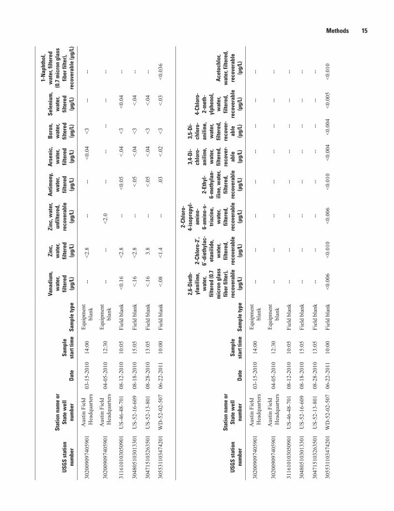
Methods 15
USG
S st
atio
n
num
ber
Stat
ion
nam
e or
St
ate
wel
l nu
mbe
rD
ate
Sam
ple
star
t tim
eSa
mpl
e ty
pe
Vana
dium
, w
ater
, fil
tere
d
(µg/
L)
Zinc
, w
ater
, fil
tere
d
(µg/
L)
Zinc
, wat
er,
unfil
tere
d,
reco
vera
ble
(µg/
L)
Ant
imon
y,
wat
er,
filte
red
(µg/
L)
Ars
enic
, w
ater
, fil
tere
d (µ
g/L)
Bor
on,
wat
er,
filte
red
(µg/
L)
Sele
nium
, w
ater
, fil
tere
d (µ
g/L)
1-N
apht
hol,
w
ater
, filt
ered
(0
.7 m
icro
n gl
ass
fiber
filte
r),
reco
vera
ble
(µg/
L)
3020
0909
7405
901
Aus
tin F
ield
H
eadq
uarte
rs03
-15-
2010
14:0
0Eq
uipm
ent
blan
k--
<2.8
----
<0.0
4<3
----
3020
0909
7405
901
Aus
tin F
ield
H
eadq
uarte
rs04
-05-
2010
12:3
0Eq
uipm
ent
blan
k--
--<2
.0--
----
----
3116
1010
3050
901
US-
46-4
8-70
108
-12-
2010
10:0
5Fi
eld
blan
k<0
.16
<2.8
--<0
.05
<.04
<3<0
.04
--
3048
0510
3013
301
US-
52-1
6-60
908
-18-
2010
15:0
5Fi
eld
blan
k<.
16<2
.8--
<.05
<.04
<3<.
04--
3047
1510
3263
501
US-
52-1
3-80
108
-28-
2010
13:0
5Fi
eld
blan
k<.
163.
8--
<.05
<.04
<3<.
04--
3055
3110
3474
201
WD
-52-
02-5
0706
-22-
2011
10:0
0Fi
eld
blan
k<.
08<1
.4--
.03
<.02
<3<.
03<0
.036
USG
S st
atio
n
num
ber
Stat
ion
nam
e or
St
ate
wel
l nu
mbe
rD
ate
Sam
ple
star
t tim
eSa
mpl
e ty
pe
2,6-
Die
th-
ylan
iline
, w
ater
, fil
tere
d (0
.7
mic
ron
glas
s fib
er fi
lter)
, re
cove
rabl
e (µ
g/L)
2-Ch
loro
-2’,
6’-d
ieth
ylac
-et
anili
de,
wat
er,
filte
red,
re
cove
rabl
e (µ
g/L)
2-Ch
loro
-4-
isop
ropy
l-am
ino-
6-
amin
o-s-
tr
iazi
ne,
wat
er,
filte
red,
re
cove
rabl
e (µ
g/L)
2-Et
hyl-
6-m
ethy
lan-
iline
, wat
er,
filte
red,
re
cove
rabl
e (µ
g/L)
3,4-
Di-
chlo
ro-
anili
ne,
wat
er,
filte
red,
re
cove
r-ab
le
(µg/
L)
3,5-
Di-
chlo
ro-
anili
ne,
wat
er,
filte
red,
re
cove
r-ab
le
(µg/
L)
4-Ch
loro
-2-
met
h-yl
phen
ol,
wat
er,
filte
red,
re
cove
rabl
e (µ
g/L)
Ace
toch
lor,
w
ater
, filt
ered
, re
cove
rabl
e
(µg/
L)
3020
0909
7405
901
Aus
tin F
ield
H
eadq
uarte
rs03
-15-
2010
14:0
0Eq
uipm
ent
blan
k--
----
----
----
--
3020
0909
7405
901
Aus
tin F
ield
H
eadq
uarte
rs04
-05-
2010
12:3
0Eq
uipm
ent
blan
k--
----
----
----
--
3116
1010
3050
901
US-
46-4
8-70
108
-12-
2010
10:0
5Fi
eld
blan
k--
----
----
----
--
3048
0510
3013
301
US-
52-1
6-60
908
-18-
2010
15:0
5Fi
eld
blan
k--
----
----
----
--
3047
1510
3263
501
US-
52-1
3-80
108
-28-
2010
13:0
5Fi
eld
blan
k--
----
----
----
--
3055
3110
3474
201
WD
-52-
02-5
0706
-22-
2011
10:0
0Fi
eld
blan
k<0
.006
<0.0
10<0
.006
<0.0
10<0
.004
<0.0
04<0
.005
<0.0
10

16 Data Collection and Compilation for a Geodatabase, Pecos County Region, Texas, 1930–2011
USG
S st
atio
n
num
ber
Stat
ion
nam
e or
St
ate
wel
l nu
mbe
rD
ate
Sam
ple
star
t tim
eSa
mpl
e ty
pe
Ala
chlo
r,
wat
er,
filte
red,
re
cove
rabl
e (µ
g/L)
alph
a-En
do-
sulfa
n, w
ater
, fil
tere
d,
reco
vera
ble
(µg/
L)
Atr
azin
e,
wat
er,
filte
red,
re
cove
rabl
e (µ
g/L)
Azi
npho
s-m
ethy
l ox
ygen
an
alog
, w
ater
, fil
tere
d,
reco
vera
ble
(µg/
L)
Azi
npho
s-m
ethy
l, w
ater
, fil
tere
d (0
.7
mic
ron
glas
s fib
er
filte
r),
reco
ver-
able
(µg/
L)
Ben
flura
-lin
, wat
er,
filte
red
(0.7
mi-
cron
gla
ss
fiber
fil
ter)
, re
cove
r-ab
le (µ
g/L)
Carb
aryl
, w
ater
, fil
tere
d (0
.7 m
icro
n gl
ass
fiber
filte
r),
reco
vera
ble
(µg/
L)
Carb
ofur
an,
wat
er, f
ilter
ed
(0.7
mic
ron
gl
ass
fiber
fil
ter)
, re
cove
rabl
e
(µg/
L)
3020
0909
7405
901
Aus
tin F
ield
H
eadq
uarte
rs03
-15-
2010
14:0
0Eq
uipm
ent
blan
k--
----
----
----
--
3020
0909
7405
901
Aus
tin F
ield
H
eadq
uarte
rs04
-05-
2010
12:3
0Eq
uipm
ent
blan
k--
----
----
----
--
3116
1010
3050
901
US-
46-4
8-70
108
-12-
2010
10:0
5Fi
eld
blan
k--
----
----
----
--
3048
0510
3013
301
US-
52-1
6-60
908
-18-
2010
15:0
5Fi
eld
blan
k--
----
----
----
--
3047
1510
3263
501
US-
52-1
3-80
108
-28-
2010
13:0
5Fi
eld
blan
k--
----
----
----
--
3055
3110
3474
201
WD
-52-
02-5
0706
-22-
2011
10:0
0Fi
eld
blan
k<0
.008
<0.0
06<0
.008
<0.0
4<0
.120
<0.0
14<0
.060
<0.0
60
Tabl
e 4.
Re
sults
of m
ajor
ion,
trac
e el
emen
t, an
d nu
trien
t ana
lyse
s fro
m e
quip
men
t bla
nks
and
field
bla
nks
colle
cted
in a
ssoc
iatio
n w
ith g
eoch
emic
al s
ampl
es c
olle
cted
in
the
Peco
s Co
unty
regi
on, T
exas
, 201
0–11
.—Co
ntin
ued
[USG
S, U
.S. G
eolo
gica
l Sur
vey;
mg/
L, m
illig
ram
s per
lite
r; µg
/L, m
icro
gram
s per
lite
r; --
, no
data
; <, l
ess t
han;
E, e
stim
ated
; M, p
rese
nce
verifi
ed b
ut n
ot q
uant
ified
; U, a
naly
zed
for b
ut n
ot d
etec
ted
at a
co
ncen
tratio
n eq
ual t
o or
gre
ater
than
the
long
-term
met
hod
dete
ctio
n le
vel]

Methods 17
USG
S st
atio
n
num
ber
Stat
ion
nam
e or
St
ate
wel
l nu
mbe
rD
ate
Sam
ple
star
t tim
eSa
mpl
e ty
pe
Chlo
rpyr
ifos
oxyg
en
anal
og,
wat
er,
filte
red,
re
cove
rabl
e (µ
g/L)
Chlo
rpyr
ifos,
w
ater
, fil
tere
d,
reco
vera
ble
(µg/
L)
cis-
Pe
rmet
hrin
, w
ater
, fil
tere
d
(0.7
mic
ron
glas
s fib
er
filte
r),
reco
vera
ble
(µg/
L)
cis-
Pr
opic
on-
azol
e,
wat
er,
filte
red,
re
cove
rabl
e (µ
g/L)
Cyan
azin
e,
wat
er,
filte
red,
re
cove
r-ab
le
(µg/
L)
Cyflu
thri
n,
wat
er,
filte
red,
re
cove
r-ab
le
(µg/
L)
Cype
rme-
thri
n,
wat
er,
filte
red,
re
cove
rabl
e (µ
g/L)
DCP
A, w
ater
, fil
tere
d
(0.7
mic
ron
gl
ass
fiber
fil
ter)
, re
cove
rabl
e
(µg/
L)
3020
0909
7405
901
Aus
tin F
ield
H
eadq
uarte
rs03
-15-
2010
14:0
0Eq
uipm
ent
blan
k--
----
----
----
--
3020
0909
7405
901
Aus
tin F
ield
H
eadq
uarte
rs04
-05-
2010
12:3
0Eq
uipm
ent
blan
k--
----
----
----
--
3116
1010
3050
901
US-
46-4
8-70
108
-12-
2010
10:0
5Fi
eld
blan
k--
----
----
----
--
3048
0510
3013
301
US-
52-1
6-60
908
-18-
2010
15:0
5Fi
eld
blan
k--
----
----
----
--
3047
1510
3263
501
US-
52-1
3-80
108
-28-
2010
13:0
5Fi
eld
blan
k--
----
----
----
--
3055
3110
3474
201
WD
-52-
02-5
0706
-22-
2011
10:0
0Fi
eld
blan
k<0
.06
<0.0
04<0
.010
<0.0
08<0
.022
<0.0
16<0
.020
<0.0
08
USG
S st
atio
n
num
ber
Stat
ion
nam
e or
St
ate
wel
l nu
mbe
rD
ate
Sam
ple
star
t tim
eSa
mpl
e ty
pe
Des
ulfi-
nylfi
pron
il am
ide,
w
ater
, fil
tere
d,
reco
vera
ble
(µg/
L)
Des
ulfin
yl-
fipro
nil,
w
ater
, fil
tere
d,
reco
vera
ble
(µg/
L)
Dia
zino
n,
wat
er,
filte
red,
re
cove
rabl
e (µ
g/L)
Dic
hlor
vos,
w
ater
, fil
tere
d,
reco
vera
ble
(µg/
L)
Dic
ro-
toph
os,
wat
er,
filte
red,
re
cove
r-ab
le
(µg/
L)
Die
ldri
n,
wat
er,
filte
red,
re
cove
r-ab
le
(µg/
L)
Dim
etho
-at
e, w
ater
, fil
tere
d (0
.7 m
icro
n gl
ass
fiber
filte
r),
reco
vera
ble
(µg/
L)
Dis
ulfo
ton
sulfo
ne, w
ater
, fil
tere
d,
reco
vera
ble
(µ
g/L)
3020
0909
7405
901
Aus
tin F
ield
H
eadq
uarte
rs03
-15-
2010
14:0
0Eq
uipm
ent
blan
k--
----
----
----
--
3020
0909
7405
901
Aus
tin F
ield
H
eadq
uarte
rs04
-05-
2010
12:3
0Eq
uipm
ent
blan
k--
----
----
----
--
3116
1010
3050
901
US-
46-4
8-70
108
-12-
2010
10:0
5Fi
eld
blan
k--
----
----
----
--
3048
0510
3013
301
US-
52-1
6-60
908
-18-
2010
15:0
5Fi
eld
blan
k--
----
----
----
--
3047
1510
3263
501
US-
52-1
3-80
108
-28-
2010
13:0
5Fi
eld
blan
k--
----
----
----
--
3055
3110
3474
201
WD
-52-
02-5
0706
-22-
2011
10:0
0Fi
eld
blan
k<0
.029
<0.0
12<0
.006
<0.0
4<0
.08
<0.0
08<0
.006
<0.0
1

18 Data Collection and Compilation for a Geodatabase, Pecos County Region, Texas, 1930–2011
USG
S st
atio
n
num
ber
Stat
ion
nam
e or
St
ate
wel
l nu
mbe
rD
ate
Sam
ple
star
t tim
eSa
mpl
e ty
pe
Dis
ulfo
ton,
w
ater
, fil
tere
d
(0.7
mic
ron
glas
s fib
er
filte
r),
reco
vera
ble
(µg/
L)
Endo
sulfa
n su
lfate
, w
ater
, fil
tere
d,
reco
vera
ble
(µg/
L)
EPTC
, w
ater
, fil
tere
d
(0.7
mic
ron
glas
s fib
er
filte
r),
reco
vera
ble
(µg/
L)
Ethi
on
mon
oxon
, w
ater
, fil
tere
d,
reco
vera
ble
(µg/
L)
Ethi
on,
wat
er,
filte
red,
re
cove
r-ab
le
(µg/
L)
Etho
prop
, w
ater
, fil
tere
d (0
.7
mic
ron
glas
s fib
er
filte
r),
reco
ver-
able
(µg/
L)
Fena
mip
hos
sulfo
ne,
wat
er,
filte
red,
re
cove
rabl
e (µ
g/L)
Fena
mip
hos
sulfo
xide
, wat
er,
filte
red,
re
cove
rabl
e
(µg/
L)
3020
0909
7405
901
Aus
tin F
ield
H
eadq
uarte
rs03
-15-
2010
14:0
0Eq
uipm
ent
blan
k--
----
----
----
--
3020
0909
7405
901
Aus
tin F
ield
H
eadq
uarte
rs04
-05-
2010
12:3
0Eq
uipm
ent
blan
k--
----
----
----
--
3116
1010
3050
901
US-
46-4
8-70
108
-12-
2010
10:0
5Fi
eld
blan
k--
----
----
----
--
3048
0510
3013
301
US-
52-1
6-60
908
-18-
2010
15:0
5Fi
eld
blan
k--
----
----
----
--
3047
1510
3263
501
US-
52-1
3-80
108
-28-
2010
13:0
5Fi
eld
blan
k--
----
----
----
--
3055
3110
3474
201
WD
-52-
02-5
0706
-22-
2011
10:0
0Fi
eld
blan
k<0
.04
<0.0
16<0
.006
<0.0
2<0
.008
<0.0
16<0
.054
<0.0
8
USG
S st
atio
n
num
ber
Stat
ion
nam
e or
St
ate
wel
l nu
mbe
rD
ate
Sam
ple
star
t tim
eSa
mpl
e ty
pe
Fena
mip
hos,
w
ater
, fil
tere
d,
reco
vera
ble
(µg/
L)
Fipr
onil
sulfi
de,
wat
er,
filte
red,
re
cove
rabl
e (µ
g/L)
Fipr
onil
su
lfone
, w
ater
, fil
tere
d,
reco
vera
ble
(µg/
L)
Fipr
onil,
w
ater
, fil
tere
d,
reco
vera
ble
(µg/
L)
Fono
fos,
w
ater
, fil
tere
d,
reco
ver-
able
(µ
g/L)
Hex
a-zi
none
, w
ater
, fil
tere
d,
reco
ver-
able
(µ
g/L)
Ipro
dion
e,
wat
er,
filte
red,
re
cove
rabl
e (µ
g/L)
Isof
enph
os,
wat
er, f
ilter
ed,
reco
vera
ble
(µ
g/L)
3020
0909
7405
901
Aus
tin F
ield
H
eadq
uarte
rs03
-15-
2010
14:0
0Eq
uipm
ent
blan
k--
----
----
----
--
3020
0909
7405
901
Aus
tin F
ield
H
eadq
uarte
rs04
-05-
2010
12:3
0Eq
uipm
ent
blan
k--
----
----
----
--
3116
1010
3050
901
US-
46-4
8-70
108
-12-
2010
10:0
5Fi
eld
blan
k--
----
----
----
--
3048
0510
3013
301
US-
52-1
6-60
908
-18-
2010
15:0
5Fi
eld
blan
k--
----
----
----
--
3047
1510
3263
501
US-
52-1
3-80
108
-28-
2010
13:0
5Fi
eld
blan
k--
----
----
----
--
3055
3110
3474
201
WD
-52-
02-5
0706
-22-
2011
10:0
0Fi
eld
blan
k<0
.03
<0.0
12<0
.024
<0.0
18<0
.005
<0.0
08<0
.014
<0.0
06
Tabl
e 4.
Re
sults
of m
ajor
ion,
trac
e el
emen
t, an
d nu
trien
t ana
lyse
s fro
m e
quip
men
t bla
nks
and
field
bla
nks
colle
cted
in a
ssoc
iatio
n w
ith g
eoch
emic
al s
ampl
es c
olle
cted
in
the
Peco
s Co
unty
regi
on, T
exas
, 201
0–11
.—Co
ntin
ued
[USG
S, U
.S. G
eolo
gica
l Sur
vey;
mg/
L, m
illig
ram
s per
lite
r; µg
/L, m
icro
gram
s per
lite
r; --
, no
data
; <, l
ess t
han;
E, e
stim
ated
; M, p
rese
nce
verifi
ed b
ut n
ot q
uant
ified
; U, a
naly
zed
for b
ut n
ot d
etec
ted
at a
co
ncen
tratio
n eq
ual t
o or
gre
ater
than
the
long
-term
met
hod
dete
ctio
n le
vel]

Methods 19
USG
S st
atio
n
num
ber
Stat
ion
nam
e or
St
ate
wel
l nu
mbe
rD
ate
Sam
ple
star
t tim
eSa
mpl
e ty
pe
lam
bda-
Cy
halo
thri
n,
wat
er,
filte
red,
re
cove
rabl
e (µ
g/L)
Mal
aoxo
n,
wat
er,
filte
red,
re
cove
rabl
e (µ
g/L)
Mal
athi
on,
wat
er,
filte
red,
re
cove
rabl
e (µ
g/L)
Met
alax
yl,
wat
er,
filte
red,
re
cove
rabl
e (µ
g/L)
Met
hi-
dath
ion,
w
ater
, fil
tere
d,
reco
ver-
able
(µ
g/L)
Met
hyl
para
oxon
, w
ater
, fil
tere
d,
reco
ver-
able
(µ
g/L)
Met
hyl
para
thio
n,
wat
er,
filte
red
(0.7
mic
ron
glas
s fib
er fi
lter)
, re
cove
rabl
e (µ
g/L)
Met
olac
hlor
, w
ater
, filt
ered
, re
cove
rabl
e
(µg/
L)
3020
0909
7405
901
Aus
tin F
ield
H
eadq
uarte
rs03
-15-
2010
14:0
0Eq
uipm
ent
blan
k--
----
----
----
--
3020
0909
7405
901
Aus
tin F
ield
H
eadq
uarte
rs04
-05-
2010
12:3
0Eq
uipm
ent
blan
k--
----
----
----
--
3116
1010
3050
901
US-
46-4
8-70
108
-12-
2010
10:0
5Fi
eld
blan
k--
----
----
----
--
3048
0510
3013
301
US-
52-1
6-60
908
-18-
2010
15:0
5Fi
eld
blan
k--
----
----
----
--
3047
1510
3263
501
US-
52-1
3-80
108
-28-
2010
13:0
5Fi
eld
blan
k--
----
----
----
--
3055
3110
3474
201
WD
-52-
02-5
0706
-22-
2011
10:0
0Fi
eld
blan
k<0
.010
<0.0
22<0
.016
<0.0
14<0
.012
<0.0
1<0
.008
<0.0
20
USG
S st
atio
n
num
ber
Stat
ion
nam
e or
St
ate
wel
l nu
mbe
rD
ate
Sam
ple
star
t tim
eSa
mpl
e ty
pe
Met
ribu
zin,
w
ater
, fil
tere
d,
reco
vera
ble
(µg/
L)
Mol
inat
e,
wat
er,
filte
red
(0.7
m
icro
n gl
ass
fiber
filte
r),
reco
vera
ble
(µg/
L)
Myc
lobu
tani
l, w
ater
, fil
tere
d,
reco
vera
ble
(µg/
L)
Oxy
fluor
fen,
w
ater
, fil
tere
d,
reco
vera
ble
(µg/
L)
Pend
i-m
etha
lin,
wat
er,
filte
red
(0.7
m
icro
n gl
ass
fiber
fil
ter)
, re
cove
r-ab
le (µ
g/L)
Phor
ate
oxyg
en
anal
og,
wat
er,
filte
red,
re
cove
r-ab
le
(µg/
L)
Phor
ate,
w
ater
, fil
tere
d (0
.7 m
icro
n gl
ass
fiber
filte
r),
reco
vera
ble
(µg/
L)
Phos
met
oxy
gen
anal
og, w
ater
, fil
tere
d,
reco
vera
ble
(µ
g/L)
3020
0909
7405
901
Aus
tin F
ield
H
eadq
uarte
rs03
-15-
2010
14:0
0Eq
uipm
ent
blan
k--
----
----
----
--
3020
0909
7405
901
Aus
tin F
ield
H
eadq
uarte
rs04
-05-
2010
12:3
0Eq
uipm
ent
blan
k--
----
----
----
--
3116
1010
3050
901
US-
46-4
8-70
108
-12-
2010
10:0
5Fi
eld
blan
k--
----
----
----
--
3048
0510
3013
301
US-
52-1
6-60
908
-18-
2010
15:0
5Fi
eld
blan
k--
----
----
----
--
3047
1510
3263
501
US-
52-1
3-80
108
-28-
2010
13:0
5Fi
eld
blan
k--
----
----
----
--
3055
3110
3474
201
WD
-52-
02-5
0706
-22-
2011
10:0
0Fi
eld
blan
k<0
.012
<0.0
04<0
.010
<0.0
06<0
.012
<0.0
3<0
.020
<0.0
5

20 Data Collection and Compilation for a Geodatabase, Pecos County Region, Texas, 1930–2011
USG
S st
atio
n
num
ber
Stat
ion
nam
e or
St
ate
wel
l nu
mbe
rD
ate
Sam
ple
star
t tim
eSa
mpl
e ty
pe
Phos
met
, w
ater
, fil
tere
d,
reco
vera
ble
(µg/
L)
Prom
eton
, w
ater
, fil
tere
d,
reco
vera
ble
(µg/
L)
Prom
etry
n,
wat
er,
filte
red,
re
cove
rabl
e (µ
g/L)
Prop
anil,
w
ater
, fil
tere
d
(0.7
mic
ron
glas
s fib
er fi
lter)
, re
cove
rabl
e (µ
g/L)
Prop
ar-
gite
, w
ater
, fil
tere
d (0
.7
mic
ron
glas
s fib
er
filte
r),
reco
ver-
able
(µ
g/L)
Sim
azin
e,
wat
er,
filte
red,
re
cove
r-ab
le
(µg/
L)
Tebu
thi-
uron
, w
ater
, fil
tere
d (0
.7 m
icro
n gl
ass
fiber
filte
r),
reco
vera
ble
(µg/
L)
Teflu
thri
n,
wat
er, f
ilter
ed,
reco
vera
ble
(µ
g/L)
3020
0909
7405
901
Aus
tin F
ield
H
eadq
uarte
rs03
-15-
2010
14:0
0Eq
uipm
ent
blan
k--
----
----
----
--
3020
0909
7405
901
Aus
tin F
ield
H
eadq
uarte
rs04
-05-
2010
12:3
0Eq
uipm
ent
blan
k--
----
----
----
--
3116
1010
3050
901
US-
46-4
8-70
108
-12-
2010
10:0
5Fi
eld
blan
k--
----
----
----
--
3048
0510
3013
301
US-
52-1
6-60
908
-18-
2010
15:0
5Fi
eld
blan
k--
----
----
----
--
3047
1510
3263
501
US-
52-1
3-80
108
-28-
2010
13:0
5Fi
eld
blan
k--
----
----
----
--
3055
3110
3474
201
WD
-52-
02-5
0706
-22-
2011
10:0
0Fi
eld
blan
k<0
.140
<0.0
12<0
.006
<0.0
10<0
.02
<0.0
06<0
.03
<0.0
10
Tabl
e 4.
Re
sults
of m
ajor
ion,
trac
e el
emen
t, an
d nu
trien
t ana
lyse
s fro
m e
quip
men
t bla
nks
and
field
bla
nks
colle
cted
in a
ssoc
iatio
n w
ith g
eoch
emic
al s
ampl
es c
olle
cted
in
the
Peco
s Co
unty
regi
on, T
exas
, 201
0–11
.—Co
ntin
ued
[USG
S, U
.S. G
eolo
gica
l Sur
vey;
mg/
L, m
illig
ram
s per
lite
r; µg
/L, m
icro
gram
s per
lite
r; --
, no
data
; <, l
ess t
han;
E, e
stim
ated
; M, p
rese
nce
verifi
ed b
ut n
ot q
uant
ified
; U, a
naly
zed
for b
ut n
ot d
etec
ted
at a
co
ncen
tratio
n eq
ual t
o or
gre
ater
than
the
long
-term
met
hod
dete
ctio
n le
vel]

Methods 21
USG
S st
atio
n
num
ber
Stat
ion
nam
e or
St
ate
wel
l nu
mbe
rD
ate
Sam
ple
star
t tim
eSa
mpl
e ty
pe
Terb
ufos
ox
ygen
an
alog
su
lfone
, w
ater
, fil
tere
d,
reco
vera
ble
(µg/
L)
Terb
ufos
, w
ater
, filt
ered
(0
.7 m
icro
n gl
ass
fiber
fil
ter)
, re
cove
rabl
e (µ
g/L)
Terb
uthy
la-
zine
, w
ater
, fil
tere
d,
reco
vera
ble
(µg/
L)
Thio
ben-
carb
, wat
er,
filte
red
(0
.7 m
icro
n gl
ass
fiber
filte
r),
reco
vera
ble
(µg/
L)
tran
s-Pr
opi-
cona
zole
, w
ater
, fil
tere
d,
reco
ver-
able
(µ
g/L)
Trib
upho
s,
wat
er,
filte
red,
re
cove
r-ab
le
(µg/
L)
Trifl
ural
in,
wat
er,
filte
red
(0.7
mic
ron
glas
s fib
er fi
lter)
, re
cove
rabl
e (µ
g/L)
Org
anic
ca
rbon
, wat
er,
unfil
tere
d
(mg/
L)
3020
0909
7405
901
Aus
tin F
ield
H
eadq
uarte
rs03
-15-
2010
14:0
0Eq
uipm
ent
blan
k--
----
----
----
E0.3
3020
0909
7405
901
Aus
tin F
ield
H
eadq
uarte
rs04
-05-
2010
12:3
0Eq
uipm
ent
blan
k--
----
----
----
<.6
3116
1010
3050
901
US-
46-4
8-70
108
-12-
2010
10:0
5Fi
eld
blan
k--
----
----
----
--
3048
0510
3013
301
US-
52-1
6-60
908
-18-
2010
15:0
5Fi
eld
blan
k--
----
----
----
--
3047
1510
3263
501
US-
52-1
3-80
108
-28-
2010
13:0
5Fi
eld
blan
k--
----
----
----
--
3055
3110
3474
201
WD
-52-
02-5
0706
-22-
2011
10:0
0Fi
eld
blan
k<0
.04
<0.0
2<0
.01
<0.0
16<0
.01
<0.0
18<0
.018
--
USG
S st
atio
n
num
ber
Stat
ion
nam
e or
St
ate
wel
l nu
mbe
rD
ate
Sam
ple
star
t tim
eSa
mpl
e ty
pe
Ura
nium
(n
atur
al),
w
ater
, fil
tere
d
(µg/
L)
3020
0909
7405
901
Aus
tin F
ield
H
eadq
uarte
rs03
-15-
2010
14:0
0Eq
uipm
ent
blan
k--
3020
0909
7405
901
Aus
tin F
ield
H
eadq
uarte
rs04
-05-
2010
12:3
0Eq
uipm
ent
blan
k--
3116
1010
3050
901
US-
46-4
8-70
108
-12-
2010
10:0
5Fi
eld
blan
k<0
.01
3048
0510
3013
301
US-
52-1
6-60
908
-18-
2010
15:0
5Fi
eld
blan
k<.
01
3047
1510
3263
501
US-
52-1
3-80
108
-28-
2010
13:0
5Fi
eld
blan
k<.
01
3055
3110
3474
201
WD
-52-
02-5
0706
-22-
2011
10:0
0Fi
eld
blan
k<.
004

22 Data Collection and Compilation for a Geodatabase, Pecos County Region, Texas, 1930–2011
Table 5. Relative percent differences between sequential replicate and environmental samples analyzed for major ions, trace elements, and elemental isotopes collected in the Pecos County region, Texas, 2010–11.
[USGS, U.S. Geological Survey; mg/L, milligrams per liter; µg/L, micrograms per liter; pCi/L, picocuries per liter; NTRU, Nephelometric Turbidity Ratio Unit; <, concentration was less than laboratory reporting level; --, RPD not calculated because the concentration for one or both samples in the pair was less than the laboratory reporting level]
USGS station number
Date Constituent Sequential replicate
result
Environmental result
Relative percent
differences
08437000 1/25/2011 Alkalinity, water, filtered inflection-point titration method (incremental titration method), field (mg/L as calcium carbonate)
254.0 232.0 9.05
08437000 1/25/2011 Aluminum, water, filtered (µg/L) 5.6 <5.1 --08437000 1/25/2011 Ammonia, water, filtered (µg/L) .057 .060 5.1308437000 1/25/2011 Arsenic, water, filtered (µg/L) 1.7 1.7 008437000 1/25/2011 Barium, water, filtered (µg/L) 20 20 008437000 1/25/2011 Beryllium, water, filtered (µg/L) .04 .04 008437000 1/25/2011 Bicarbonate, water, filtered, inflection-point titration
method (incremental titration method), field (mg/L)309 283 8.78
08437000 1/25/2011 Boron, water, filtered (µg/L) 1,010 1,020 0.9908437000 1/25/2011 Bromide, water, filtered (mg/L) 2.33 2.37 1.7008437000 1/25/2011 Cadmium, water, filtered (µg/L) .10 .05 66.6708437000 1/25/2011 Calcium, water, filtered (mg/L) 447 462 3.3008437000 1/25/2011 Carbonate, water, filtered, inflection-point titration method
(incremental titration method), field (mg/L).3 .2 40.00
08437000 1/25/2011 Chloride, water, filtered (mg/L) 1,180 1,180 008437000 1/25/2011 Chromium, water, filtered (µg/L) .40 .43 7.2308437000 1/25/2011 Cobalt, water, filtered (µg/L) .46 .36 24.3908437000 1/25/2011 Delta deuterium, water, unfiltered (per mil) -46.70 -47.00 -0.6408437000 1/25/2011 Delta oxygen-18, water, unfiltered (per mil) -6.57 -6.56 -0.1508437000 1/25/2011 Dissolved solids dried at 180 degrees Celsius, water,
filtered (mg/L)4,530 4,520 0.22
08437000 1/25/2011 Fluoride, water, filtered (mg/L) 1.70 1.72 1.1708437000 1/25/2011 Iron, water, filtered (µg/L) 15 <13 --08437000 1/25/2011 Lead, water, filtered (µg/L) 0.11 <0.04 --08437000 1/25/2011 Lithium, water, filtered (µg/L) 280 279 0.3608437000 1/25/2011 Magnesium, water, filtered (mg/L) 176 180 2.2508437000 1/25/2011 Manganese, water, filtered (µg/L) 12.8 12.5 2.3708437000 1/25/2011 Molybdenum, water, filtered (µg/L) 13.7 13.7 008437000 1/25/2011 Nickel, water, filtered (µg/L) 2.0 1.9 5.1308437000 1/25/2011 Nitrite, water, filtered (µg/L) .02 .02 008437000 1/25/2011 Nitrate plus Nitrite, water, filtered (mg/L) 2.97 2.95 0.6808437000 1/25/2011 Orthophosphate, water, filtered (mg/L as phosphorus) .02 .02 008437000 1/25/2011 Potassium, water, filtered (mg/L) 21.1 21.6 2.3408437000 1/25/2011 Selenium, water, filtered (µg/L) 5.4 5.6 3.6408437000 1/25/2011 Silica, water, filtered (mg/L as SiO2) 32.4 32.8 1.2308437000 1/25/2011 Silver, water, filtered (µg/L) <.01 .02 --08437000 1/25/2011 Sodium, water, filtered (mg/L) 688 696 1.1608437000 1/25/2011 Strontium, water, filtered (µg/L) 8,760 9,060 3.3708437000 1/25/2011 Sulfate, water, filtered (mg/L) 1,550 1,550 0

Methods 23
08437000 1/25/2011 Thallium, water, filtered (µg/L) 0.28 0.26 7.4108437000 1/25/2011 Total nitrogen, water, filtered (mg/L) 3.09 3.16 2.2408437000 1/25/2011 Tritium, water, unfiltered (pCi/L) 1.9 1.8 5.4108437000 1/25/2011 Uranium (natural), water, filtered (µg/L) 21.0 21.1 0.4808437000 1/25/2011 Vanadium, water, filtered (µg/L) 6.3 6.5 3.13304006103315601 6/23/2011 Alkalinity, water, filtered inflection-point titration method
(incremental titration method), field (mg/L as calcium carbonate)
330 336 1.80
304006103315601 6/23/2011 Ammonia, water, filtered (µg/L) .781 .780 0.13304006103315601 6/23/2011 Antimony, water, filtered (µg/L) <.03 .13 --304006103315601 6/23/2011 Arsenic, water, filtered (µg/L) 3.1 3.0 3.28304006103315601 6/23/2011 Barium, water, filtered (µg/L) 40 40 0304006103315601 6/23/2011 Beryllium, water, filtered (µg/L) .02 .02 0304006103315601 6/23/2011 Bicarbonate, water, filtered, inflection-point titration
method (incremental titration method), field (mg/L)401 409 1.98
304006103315601 6/23/2011 Boron, water, filtered (µg/L) 1,120 1,110 0.90304006103315601 6/23/2011 Cadmium, water, filtered (µg/L) .03 .03 0304006103315601 6/23/2011 Calcium, water, filtered (mg/L) 26.8 27.0 0.74304006103315601 6/23/2011 Carbonate, water, filtered, inflection-point titration method
(incremental titration method), field (mg/L).7 .6 15.38
304006103315601 6/23/2011 Chloride, water, filtered (mg/L) 57.1 58.6 2.59304006103315601 6/23/2011 Cobalt, water, filtered (µg/L) .07 <0.02 --304006103315601 6/23/2011 Dissolved solids dried at 180 degrees Celsius, water,
filtered (mg/L)869 859 1.16
304006103315601 6/23/2011 Fluoride, water, filtered (mg/L) 1.22 1.23 0.82304006103315601 6/23/2011 Iron, water, filtered (µg/L) 66 65 1.53304006103315601 6/23/2011 Lead, water, filtered (µg/L) .02 1.21 193.50304006103315601 6/23/2011 Lithium, water, filtered (µg/L) 198 199 0.50304006103315601 6/23/2011 Magnesium, water, filtered (mg/L) 4.39 4.38 0.23304006103315601 6/23/2011 Manganese, water, filtered (µg/L) 15.9 16.1 1.25304006103315601 6/23/2011 Molybdenum, water, filtered (µg/L) 12.5 12.5 0304006103315601 6/23/2011 Orthophosphate, water, filtered (mg/L as phosphorus) .019 .019 0304006103315601 6/23/2011 Potassium, water, filtered (mg/L) 7.25 7.43 2.45304006103315601 6/23/2011 Selenium, water, filtered (µg/L) .06 .06 0304006103315601 6/23/2011 Silica, water, filtered (mg/L as SiO2) 20.7 21.1 1.91304006103315601 6/23/2011 Sodium, water, filtered (mg/L) 266 265 0.38304006103315601 6/23/2011 Strontium, water, filtered (µg/L) 1,020 1,030 0.98304006103315601 6/23/2011 Sulfate, water, filtered (mg/L) 271 271 0304006103315601 6/23/2011 Total nitrogen, water, filtered (mg/L) .85 .86 1.17304006103315601 6/23/2011 Uranium (natural), water, filtered (µg/L) 22.4 22.4 0304006103315601 6/23/2011 Vanadium, water, filtered (µg/L) .19 .21 10.00
Table 5. Relative percent differences between sequential replicate and environmental samples analyzed for major ions, trace elements, and elemental isotopes collected in the Pecos County region, Texas, 2010–11.—Continued
[USGS, U.S. Geological Survey; mg/L, milligrams per liter; µg/L, micrograms per liter; pCi/L, picocuries per liter; NTRU, Nephelometric Turbidity Ratio Unit; <, concentration was less than laboratory reporting level; --, RPD not calculated because the concentration for one or both samples in the pair was less than the laboratory reporting level]
USGS station number
Date Constituent Sequential replicate
result
Environmental result
Relative percent
differences

24 Data Collection and Compilation for a Geodatabase, Pecos County Region, Texas, 1930–2011
304006103315601 6/23/2011 Zinc, water, filtered (µg/L) 2.6 3.0 14.29305331103020501 8/17/2010 Alkalinity, water, filtered inflection-point titration method
(incremental titration method), field (mg/L as calcium carbonate)
230 235 2.15
305331103020501 8/17/2010 Arsenic, water, filtered (µg/L) .60 .56 6.90305331103020501 8/17/2010 Barium, water, filtered (µg/L) 15 16 6.45305331103020501 8/17/2010 Bicarbonate, water, filtered, inflection-point titration
method (incremental titration method), field (mg/L)280 286 2.12
305331103020501 8/17/2010 Boron, water, filtered (µg/L) 388.8 396.4 1.94305331103020501 8/17/2010 Bromide, water, filtered (mg/L) 1.06 1.05 0.95305331103020501 8/17/2010 Calcium, water, filtered (mg/L) 275 278 1.08305331103020501 8/17/2010 Carbonate, water, filtered, inflection-point titration method
(incremental titration method), field (mg/L).2 .2 0
305331103020501 8/17/2010 Chloride, water, filtered (mg/L) 760 758 0.26305331103020501 8/17/2010 Cobalt, water, filtered (µg/L) .11 .11 0305331103020501 8/17/2010 Delta deuterium, water, unfiltered (per mil) -50.50 -52.30 -3.50305331103020501 8/17/2010 Delta oxygen-18, water, unfiltered (per mil) -7.41 -7.47 -0.81305331103020501 8/17/2010 Dissolved solids dried at 180 degrees Celsius, water,
filtered (mg/L)2,770 2,770 0
305331103020501 8/17/2010 Fluoride, water, filtered (mg/L) 1.31 1.30 0.77305331103020501 8/17/2010 Lead, water, filtered (µg/L) .19 .19 0305331103020501 8/17/2010 Lithium, water, filtered (µg/L) 130 133 2.28305331103020501 8/17/2010 Magnesium, water, filtered (mg/L) 107 109 1.85305331103020501 8/17/2010 Molybdenum, water, filtered (µg/L) 14.2 14.5 2.09305331103020501 8/17/2010 Nickel, water, filtered (µg/L) .88 .83 5.85305331103020501 8/17/2010 Nitrate plus Nitrite, water, filtered (mg/L) 1.63 1.61 1.23305331103020501 8/17/2010 Orthophosphate, water, filtered (mg/L as phosphorus) .016 .018 11.76305331103020501 8/17/2010 Potassium, water, filtered (mg/L) 15.0 15.2 1.32305331103020501 8/17/2010 Selenium, water, filtered (µg/L) 3.6 3.7 2.74305331103020501 8/17/2010 Silica, water, filtered (mg/L as SiO2) 23.4 23.3 0.43305331103020501 8/17/2010 Sodium, water, filtered (mg/L) 418 421 0.72305331103020501 8/17/2010 Strontium, water, filtered (µg/L) 5,490 5,330 2.96305331103020501 8/17/2010 Sulfate, water, filtered (mg/L) 912 908 0.44305331103020501 8/17/2010 Thallium, water, filtered (µg/L) .87 .87 0305331103020501 8/17/2010 Total nitrogen, water, filtered (mg/L) 1.61 1.61 0305331103020501 8/17/2010 Tritium, water, unfiltered (pCi/L) 1.5 1.3 14.29305331103020501 8/17/2010 Uranium (natural), water, filtered (µg/L) 8.76 8.90 1.59305331103020501 8/17/2010 Vanadium, water, filtered (µg/L) 1.8 1.9 5.41305509103510101 9/1/2010 Delta deuterium, water, unfiltered (per mil) -11.70 -11.50 -1.72305509103510101 9/1/2010 Delta oxygen-18, water, unfiltered (per mil) -0.52 -0.61 -15.93
Table 5. Relative percent differences between sequential replicate and environmental samples analyzed for major ions, trace elements, and elemental isotopes collected in the Pecos County region, Texas, 2010–11.—Continued
[USGS, U.S. Geological Survey; mg/L, milligrams per liter; µg/L, micrograms per liter; pCi/L, picocuries per liter; NTRU, Nephelometric Turbidity Ratio Unit; <, concentration was less than laboratory reporting level; --, RPD not calculated because the concentration for one or both samples in the pair was less than the laboratory reporting level]
USGS station number
Date Constituent Sequential replicate
result
Environmental result
Relative percent
differences

Methods 25
Field spikes are used to assess bias and variability from degradation of organic constituent concentrations during sample processing, storage, and analysis. Field spikes are environmental replicate samples into which a known volume and concentration of target analytes are added. Analytical recoveries of the spiked target compounds are expressed as percentages of expected (theoretical) concentrations. Computed field-spike recoveries (equation 2) are compared to theoretical and laboratory recoveries to evaluate matrix interferences or degradation of organic compounds:
Recovery = [(Cspiked – Cunspiked) ÷ Cexpected] × 100, (2)
where Cspiked is the measured concentration of analyte
in the spiked environmental sample, in micrograms per liter;
Cunspiked is the measured concentration of analyte in the unspiked environmental sample, in micrograms per liter;
Cexpected is the theoretical concentration of analyte in the spiked environmental sample, in micrograms per liter, and is computed as
Cexpected = Csolution × Vspike ÷ Vsample, (3)
where Csolution is concentration of analyte in spiked
environmental solution, in micrograms per liter;
Vspike is volume of spike added to environmental sample, in milliliters; and
Vsample is volume of environmental sample, in liters.
A mixture of target analytes was added to a replicate environmental sample (site 305419102545301 collected on August 6, 2010). The calculated spike recoveries in this report were compared to time-series graph of groundwater spike recoveries in appendix 3 of Martin and Eberle (2011). In 2010, the spike recoveries in this report are within the range of spike recoveries shown by Martin and Eberle, indicating no bias in the results. For target analytes not included, the spiked recoveries of reagent water by the NWQL were reviewed for method performance, with methods appearing to be operating normally (U.S. Geological Survey, 2012).
Geophysical Methods
Surface and borehole geophysical data were collected throughout the study area from 2009 to 2011 to supplement compiled historical data and to minimize data gaps. Time-domain electromagnetic (TDEM) soundings were collected at 4 locations (fig. 4, table 6) and audio-magnetotelluric (AMT)
soundings were collected at 13 locations (fig. 4, table 7) and borehole geophysical logs were collected at 44 locations (fig. 4, table 8). Site locations and associated information can be accessed using the USGS NWIS (U.S. Geological Survey, 2011a) and archived geophysical database.
Surface Geophysical Methods
Surface geophysical resistivity methods can be used to detect changes in the electrical properties of the subsurface (Zohdy and others, 1974). The electrical properties of soil and rock are determined by water content, porosity, clay content and mineralogy, and conductivity (or reciprocal of electri-cal resistivity) of the pore water (Lucius and others, 2007). Resistivity measurements can be used to construct graphical images of the spatial distribution of electrical properties of the subsurface which, in turn, can be used to identify stratigraphic units and describe subsurface hydrogeology. The two surface geophysical methods used to evaluate the subsurface stratigraphy and hydrogeology in the study area were TDEM and AMT. Comprehensive descrip tions of the theory and application of surface geophysical resistivity methods, as well as tables of the electrical properties of earth materials, are presented in Keller and Frischknecht (1966) and Lucius and others (2007).
Time-Domain Electromagnetic Soundings
Four TDEM soundings were collected at four different sites using the Geonics Protem 47 and 57 systems (Geonics Limited, 2006a,b). Each of the locations were near wells that had borehole geophysical logs collected by the USGS. Locations were selected so that the TDEM could be compared to the borehole geophysical logs to determine if this geophysical method would yield information to fill in data gaps associated with these sites.
The Geonics Protem 47 and 57 systems (hereinafter referred to as Protem 47 and 57, respectively) were used to collect TDEM soundings at each site. The Protem 47 and 57 use a multi turn receiver (Rx) coil to measure electromagnetic fields in the center of the transmitter (Tx) loop. The effective area of the receiver relates to the sensitivity of the Rx coil. The 100 square meter (m2) Rx coil of the Protem 57 is able to measure smaller voltages than the 31.4-m2 coil of the Protem 47. At each sounding, an integration time of 15 seconds (s) was used to measure six different data sets (the compilation of these data sets is referred to as a stack). The mean value of all the soundings collected over the integration time is stored. The values stored in the stack are averaged to ensure data quality and repeatability, and averaging is done prior to the inversion step, which is explained in the inverse modeling section of this report.

26 Data Collection and Compilation for a Geodatabase, Pecos County Region, Texas, 1930–2011
31°0
'
30°3
0'
102°
30'
103°
0'
103°
30'
Peco
s Riv
er
Peco
s Riv
er
RE
EV
ES
CO
UN
TY
WA
RD
CO
UN
TY
CR
AN
EC
OU
NT
Y
UPT
ON
CO
UN
TY
PEC
OS
CO
UN
TY
JEFF
DAV
ISC
OU
NT
Y
BR
EW
STE
RC
OU
NT
Y
TE
RR
EL
LC
OU
NT
Y
CR
OC
KE
TT
CO
UN
TY
3037
1710
3214
801
3038
5210
2432
901
3026
3010
2503
801
3039
4810
3205
801
3021
2510
3022
801
3037
1810
3214
601
3038
2410
2285
001
3050
4210
2595
60130
4620
1030
1510
1
3051
1010
2533
401
3052
3410
2504
301
3055
4810
3161
401
3045
5110
2361
201
3050
5510
3110
801
3035
0310
2303
601
3041
3410
2312
601
3047
1110
3003
301
3047
1510
3263
501
3047
2810
2304
401
3114
3410
2384
801
3046
2210
2312
401
3053
5710
2172
001
3112
4410
2451
401
3 100
4110
2152
901
3056
2710
3071
901
3057
1510
2571
401
3053
2310
2530
201
3054
1610
2184
801
3053
3610
2361
801
3054
0410
2512
701
3108
0610
3171
901
3042
1010
2443
201
3057
4010
3110
901
3111
2410
2302
201
3057
0610
2095
501
3102
3810
3191
701
3058
3510
2134
701
3111
0010
3080
50131
1235
1030
0090
1
3021
2210
2504
501
3041
5310
3090
501
3056
0410
2581
301
3116
2510
2403
901
3116
1510
3035
101
AM
T#13
AM
T#10
AM
T#9
AM
T#6
AM
T#5
AM
T#4
AM
T#3
AM
T#2
AM
T#1
AM
T#8
AM
T#7
AM
T#11
AM
T#12
TDEM
#4
TDEM
#2TD
E M#1
TDEM
#3
Fort
Stoc
kton
Gra
ndfa
lls
Girv
in
EXPL
AN
ATIO
NSt
udy
area
bou
ndar
yG
eoch
emic
al s
ampl
ing
site
Bor
ehol
e lo
ggin
g si
te a
nd
st
atio
n nu
mbe
r A
udio
-mag
neto
tellu
ric s
ound
ing
si
te a
nd s
ite id
entif
ier
Tim
e-do
mai
n el
ectro
mag
netic
so
undi
ng s
ite a
nd s
ite id
entif
ier
Geo
data
base
site
3102
3810
3191
701
AMT#
4
TDEM
#3 Base
mod
ified
from
U.S
. Geo
logi
cal S
urve
y 1:
2,00
0,00
0-sc
ale
digi
tal d
ata
Albe
rs E
qual
Are
a Pr
ojec
tion,
Texa
s St
ate
Map
ping
Sys
tem
Nor
th A
mer
ican
Dat
um o
f 198
3
010
20 M
ILES
515
010
20 K
ILOM
ETER
S5
15
Figu
re 4
. Si
te lo
catio
ns o
f fie
ld-c
olle
cted
geo
phys
ical
dat
a, in
clud
ing
bore
hole
logg
ing
and
surfa
ce g
eoph
ysic
al s
ites,
Pec
os C
ount
y re
gion
, Tex
as, 2
009–
11.

Methods 27
Table 6. Time-domain electromagnetic geophysical sounding sites, Pecos County region, Texas, 2009-11
[TDEM, time-domain electromagnetic; USGS, U.S. Geological Survey; dd, decimal degrees]
Sounding identification number USGS station number State well number Latitude (dd) Longitude (dd)
TDEM#1 305110102533401 US-53-09-301 30.85286 -102.89278
TDEM#2 305042102595601 US-53-09-106 30.84509 -102.99899
TDEM#3 304711103003301 US-52-16-909 30.69795 -103.15138
TDEM#4 303824102285001 US-53-21-703 30.64000 -102.48052
Table 7. Audio magnetotelluric geophysical sounding sites, Pecos County region, Texas, 2009-11.
[AMT, audio magnetotelluric; USGS, U.S.Geological Survey; dd, decimal degrees; --, sounding not collected at/near well site]
Sounding identification number USGS station number State well number Latitude (dd) Longitude (dd)
AMT#1 -- -- 30.57745 -103.28333AMT#2 -- -- 30.51932 -103.30687AMT#3 -- -- 30.71023 -103.52157AMT#4 -- -- 30.88350 -103.38389AMT#5 -- -- 30.80659 -103.48194AMT#6 -- -- 30.60335 -102.78842AMT#7 303824102285001 US-53-21-703 30.64000 -102.48052AMT#8 302630102503801 US-53-34-401 30.44176 -102.84396AMT#9 -- -- 31.06002 -103.13731AMT#10 -- -- 30.94134 -102.55057AMT#11 304622102312401 US-53-12-901 30.77304 -102.52379AMT#12 310806103171901 WD-46-54-901 31.13502 -103.28796AMT#13 -- -- 30.86516 -103.82792

28 Data Collection and Compilation for a Geodatabase, Pecos County Region, Texas, 1930–2011
Table 8. Borehole geophysical data-collection sites, Pecos County region, Texas, 2009-11.[USGS, U.S. Geological Survey; dd, decimal degrees]
USGS station number State well number Latitude (dd) Longitude (dd)
302122102504501 US-53-42-101 30.356 -102.8458611302125103022801 BK-52-48-301 30.357 -103.0411306302630102503801 US-53-34-401 30.4417611 -102.8439611303503102303601 US-53-28-303 30.5842111 -102.5100694303717103214801 US-52-30-107 30.62143889 -103.3638306303718103214601 US-52-30-108 30.62181944 -103.3632389303824102285001 US-53-21-703 30.64 -102.4805194303852102432901 US-53-19-701 30.6479 -102.7247111303948103205801 52-22-7xx 30.66344444 -103.3494444304134102312601 US-53-20-603 30.69278889 -102.5239889304153103090501 US-52-23-604 30.69795 -103.1513806304210102443201 53-19-4xx 30.70269444 -102.7422778304551102361201 US-53-12-701 30.76448056 -102.6038694304620103015101 US-53-02-7xx (COFS 6) 30.7721 -103.0308304622102312401 US-53-12-901 30.77303889 -102.5237889304711103003301 US-52-16-909 30.78641944 -103.0093194304715103263501 US-52-13-801 30.7874 -103.4434306304728102304401 US-53-12-902 30.79098056 -102.5121611305042102595601 US-53-09-106 30.84508889 -102.9989889305055103110801 52-15-2xx 30.84863889 -103.1856667305110102533401 US-53-09-301 30.8528611 -102.8927806305234102504301 US-53-02-708 30.87618056 -102.8452111305323102530201 US-53-01-908 30.88951944 -102.8839694305336102361801 US-53-04-701 30.89363889 -102.6054305357102172001 US-53-06-901 30.89923056 -102.2891194305404102512701 US-53-02-710 30.9012 -102.8577305416102184801 US-53-06-803 30.90458056 -102.3132694305548103161401 US-52-06-604 30.9302 -103.2706305604102581301 US-53-01-4xx (Apache 4) 30.93455 -102.9703305627103071901 US-52-08-402 30.94075 -103.122305706102095501 US-53-07-601 30.95175 -102.1653611305715102571401 US-53-01-503 30.9542611 -102.9538194305740103110901 US-52-07-201 30.9612 -103.1860806305835102134701 US-53-07-106 30.9765 -102.2297694310041102152901 US-45-62-901 31.0115611 -102.25855310238103191701 US-46-62-801 31.0440111 -103.3213889310806103171901 WD-46-54-901 31.13501944 -103.2879611311100103080501 US-46-55-603 31.1834611 -103.1347389311124102302201 US-45-52-602 31.19008056 -102.5065389311235103000901 US-46-56-309 31.20973889 -103.0026194311244102451401 US-45-50-302 31.21208889 -102.7539694311434102384801 US-45-51-306 31.24468056 -102.6493311615103035101 US-46-48-805 31.2708111 -103.0641611311625102403901 US-45-43-806 31.27378889 -102.6778389

Methods 29
For each TDEM sounding collected, the voltages measured from the eddy currents were averaged and evaluated statistically by using preprocessing scripts (Joe Vrabel, U.S. Geological Survey, written commun., 2010). These scripts use the raw field data (voltage data) to cal culate the uncertainty of each time gate (measured voltage values at discreet intervals of time increasing after shutoff of the cur rent) independently. After calculating the standard deviation of the voltage, the user can specify limits to trim the data set (remove outliers prior to inverse modeling). For this study, the data were initially filtered by using the mean of the six stacks collected. Outliers were evaluated by the program and any data that were more than 10 percent above or below other data points were removed. The averages of each time gate were saved as processed data files to be used in the inversion software (Interpex Limited, 1996).
Audiomagnetotelluric SoundingsA total of 13 AMT soundings was collected and
processed within the study area using the Stratagem EH4 electrical conductivity imaging system developed by Geometrics, Inc. and Electromagnetic Instruments, Inc. (Geometrics, 2012), and in accordance with techniques described by Asch and Sweetkind (2010). Of the 13 soundings collected, 4 of these soundings were collected near wells that had borehole geophysical logs collected by the USGS. These locations were selected so that the AMT soundings could be compared to the borehole geophysical logs, which aid in the interpretation of the AMT soundings. The remaining nine sounding locations were selected in areas where little or no other compiled data were located.
The Stratagem EH4 system was used to collect AMT data for each sounding location. The Stratagem EH4 system measures perpendicular arrays of electrical and magnetic fields labeled as X and Y directions within a range of 10 hertz (Hz) to 100 kilohertz (kHz) (Asch and Sweetkind, 2010). The electric field was measured by four stainless-steel electrodes placed into the earth with a 25-meter dipole (two electrodes separated by 25 meters) in the X direction and a 25-meter dipole in the Y direction. A fifth electrode was used as a ground. The ambient magnetic field was measured with two induction magnetometer coils that were placed more than 3 meters away from the electrode dipoles and are placed level in a small trench and then covered with dirt to ensure there is no movement of the coil. The controlled source transmitter was a 400-watt transmitter to supplement the received electromagnetic signal in the frequency range from 900 Hz to 23,000 Hz. The X and Y directions were chosen on a site by site basis with the X and Y directions being approximately 45 degrees from visible anthropogenic sources (Geometrics, 2007).
Time-series datasets were analyzed and selected based on the optimal signal-to-noise ratio before calculations were performed on the datasets. The measured AMT time-series
datasets at each location were converted to the frequency domain and processed to determine a two-dimensional (2D) impedance tensor of apparent resistivity and phase (Asch and Sweetkind, 2010). Poor quality (noisy) data were filtered out in the time-series datasets before the conversion was made and in the spectral and resistivity datasets after conversion. Apparent resistivity is the approximate ratio of the magnitude of the electric field to the magnitude of the magnetic field for a given frequency (Asch and Sweetkind, 2010). The impedance tensor was rotated to an angle that closely represented a 2D earth at each sounding location. This allows for the separation of the TE and TM modes, which can be used to identify lateral variation across the sounding site.
Data were exported from Imagem, the Stratagem data acquisition program, into two files: a cross-power data file, which contained spectral conversion of the data and a magnetotelluric (MT) impedance data file, which contained the apparent resistivity and phase conversion of the data (Geometrics, 2007). These files were used during the 2D inversion modeling process.
Inverse Modeling of Surface Geophysical Results
Apparent resistivity represents the resistivity of a completely uniform (homogenous and isotropic) subsurface (Keller and Frischknecht, 1966). Inverse modeling is the process of creating an estimate of the true distribution of subsurface resistivity (derived from the actual heterogeneous, anisotropic rocks) from the measured apparent resistivity (modeled as homogeneous, isotropic rocks). To estimate the resistivity of nonuniform earth material, inverse modeling software is used. The IX1Dv3 program, developed by Interpex Limited (1996), was used for inverse modeling of the TDEM soundings. The AMT sounding data were inverted using selected inversion algorithms within the Geotools MT software package used to process AMT and MT data (Geotools, 1998).
For this report, root mean square errors (RMSE) of 10 percent or less were generally considered acceptable, and RMSEs of 5 percent were generally considered good.The inverse modeling results of the TDEM data collected throughout the area had RMSEs of less than 4 percent for all soundings collected (appendix 1). The TDEM results were not able to resolve the depths needed to make geologic picks, so AMT was used to obtain deeper information.
The inverse modeling results of the AMT data collected throughout the area had acceptable errors between the measured field data and the calculated model data (appendix 2). There were two locations (AMT07 and AMT13, fig. 4) where anthropogenic noise distorted the signal sufficiently such that a poor inversion result was obtained. Four of the AMT soundings were located near wells from which geophysical logs were obtained, allowing the data quality to be assessed using borehole geophysical results.

30 Data Collection and Compilation for a Geodatabase, Pecos County Region, Texas, 1930–2011
Borehole Geophysical MethodsBorehole geophysical data such as natural gamma,
formation resistivity, and caliper are commonly used to characterize and identify stratigraphic units (Keys, 1997). Many of these data had been collected in some wells in the study area as parts of previous studies and petroleum exploration (Small, and Ozuna, 1993; Smith and others, 2000). Conventional borehole geophysical log data such as natural gamma, formation resistivity, fluid resistivity, temperature, and caliper were collected in 44 wells where additional geophysical data were most critical to supplement existing data. In addition to the conventional borehole geophysical methods, advanced borehole geophysical measurements of vertical flow (magnitude and direction), in the borehole were collected in six representative wells using the Electromagnetic (EM) flowmeter. These data can be evaluated to determine the relation of flow to the hydrostratigraphic units in each well. All borehole geophysical data were collected using a Century Geophysical Corporation System VI logging system conveyed by a 0.25-in. diameter 4-conductor wireline or a Mount Sopris Instruments Matrix logging system conveyed by a 0.1875-in. diameter single conductor wireline. Limitations, calibration procedures, and algorithms of the geophysical probes are available from the manufacturers (Century Geophysical Corporation, 2012; Mount Sopris Instruments, 2012).
Electromagnetic Induction LogsElectromagnetic induction probes measure conductivity
in air- or water-filled holes and perform well in open holes or polyvinyl chloride (PVC) cased holes. The measurement of conductivity commonly is reciprocated to provide logs with curves of resistivity and conductivity (Keys, 1997). Conductivity is affected by the salinity of borehole and formation fluids and the type of lithology encountered. Generally, pure carbonates, sands, and gravels have lower conductivity, thus higher resistivity, than clays or shales (Keys, 1997). A Century Geophysical Corporation 9510 or a Geonics EM39 induction conductivity probe was calibrated and was used to the manufacturer’s specifications (Century Geophysical Corporation, written commun., 2011; Mount Sopris Instruments, written commun., 2011). The EM induction conductivity measurements (commonly sensitive to metallic conductive objects) were affected at depths corresponding with metal objects such as centralizers and stainless steel screens.
Natural Gamma LogsNatural gamma logs provide a record of gamma
radiation detected at depth in a borehole. Fine-grained sediments that con tain abundant clay tend to be more
radioactive than quartz-grain sandstones or carbonates (Keys, 1997). The natural gamma log was run in conjunction with the fluid resistivity log and was recorded in natural gamma counts per second simultaneously as the induction log was recorded in both cased and open boreholes. A Century Geophysical Corporation 8044 multiparameter probe or a Mount Sopris Instruments 2PGA–1000 natural gamma probe with a sodium iodide detector was calibrated and was used to the manufacturer’s specifications. The natural gamma and induction logs collectively can be useful in identifying lithologies and contact depths of the strata penetrated in the borehole.
Electric LogsElectric logs use a series of electrodes mounted on the
downhole probe and a surface electrode in the ground to measure potential (or voltage) that varies with the electrical properties of fluids and rock materials. Electric logs require an uncased, fluid-filled hole to allow the current to flow into the formation. Electric logs include the following electrical methods measured in boreholes: normal resistivity, lateral resistivity, spontaneous potential, and single-point resistance. A Century Geophysical Corporation model 8044 multiparameter E-log probe was used to measure normal resistivity, lateral resistivity, spontaneous potential, and single-point resistance. These geophysical methods are explained in detail in Keys (1990, 1997).
Caliper LogsCaliper logs provide a measurement of the diameter of
the borehole and are useful in determining changes in borehole diameter that can be related to drilling techniques, cavernous formations, lithology, and well construction. The Century Geophysical Corporation model 7074 and the Mount Sopris Instruments 2PCA–1000, three-arm caliper probes were used in this study and recorded an average diameter measured by the three arms. The Century Geophysical Corporation 7074 probe was run in the short or long arm configurations (depending on hole diameter) for boreholes from 2 to 24 and 2 to 36 inches in diameter, respectively (Century Geophysical Corporation, 2012). The Mount Sopris Instruments 2PCA–1000 can be used in boreholes from 2 to 17 inches in diameter (Mount Sopris Instruments, 2012). Other limitations and algorithms of the geophysical probes can be found at Century Geophysical Corporation (2012) and Mount Sopris Instruments (2012). The caliper logs were collected using the Century Geophysical Corporation System IV or Mount Sopris Instruments Matrix logging systems. The caliper was cali-brated by performing a two-point calibration on short sections of pipe (rings) where diameters were larger and smaller than the borehole sizes that were expected to be encountered.

Methods 31
Fluid Resistivity and Temperature LogsFluid resistivity logs provide a record of the capacity
of the borehole fluid to conduct electrical current (Keys, 1990). Changes in fluid resistivity are measured by ring electrodes inside a housing that allows borehole fluid to flow through it. When feasible, fluid resistivity logs were run as the first logging run to record the ambient conditions before other probes have passed through the borehole and have vertically mixed the borehole fluid. Curve deflections on the fluid resistivity log can indicate horizontal or vertical flow, stratification of borehole fluid, or screened intervals in cased wells. The fluid resistiv ity values also can be used in calculations with other logs. Fluid resistivity and the reciprocal (fluid conductivity) are shown on the logs in this study for comparison to specific-conductance values collected at springs (appendix 1).
The fluid conductivity values contained in the logs for this study are the values recorded at the ambient borehole temperature and are not corrected to a standard tempera ture. A Century Geophysical Corporation model 8044 multiparameter E-log probe or a Mount Sopris Instruments model 2PFA–1000 probe was used to log fluid resistivity in uncased (open) boreholes and cased wells. Calibration of the fluid resistivity logging probes was done with solutions of known conductivity in a two-point calibration. Temperature logs record the temperature of the borehole fluid that the logging probe passes through as it is raised or lowered in the borehole. A Century Geophysical Corporation model 8044 multiparameter E-log probe or a Mount Sopris Instruments model 2PFA–1000 probe was used to log fluid temperature in uncased (open) boreholes and cased wells. All temperature logs were collected as the probe was lowered in the borehole to maximize the flow into the sensor housing at the bottom of the Century Geophysical Corporation model 8044 logging probe. Temperature logs can provide useful information on the movement of water through a water-well borehole, including the location of depth intervals that produce or accept water (Keys, 1990).
Optical Borehole ImagingThe optical borehole imager (OBI) is an oriented logging
device that can provide a high-resolution, 360-degree image or “cylin drical picture” of the circumference of the borehole that can be used to evaluate secondary porosity features such as fractures and solution openings. The OBI uses a digital scanning camera and conical mirror, which records a 360-degree image of the borehole wall showing the texture, color, and fractures in air-filled or clear fluid-filled boreholes (Hearst and others, 2000). A cylindrical light ring between the camera and mirror illuminates the part of the borehole wall being imaged. An Advanced Logic Technology optical borehole imager or OBI40 was used to collect optical images
of the surface wall of open and cased wells in both air and clear water (Advanced Logic Technology, 2012). The utility and analytical methods of optical imaging are explained in Keys (1997) and Hearst and others (2000).
Acoustic Borehole Imaging
The acoustic borehole imager (ABI) is an oriented logging device that can provide a high-resolution, 360-degree image or cylin drical acoustic image of the circumference of the borehole that can be used to evaluate secondary porosity features such as fractures and solution openings. Acoustic borehole imaging tools generate an image of the borehole wall by transmitting ultrasonic pulses from a rotating sensor and recording the amplitude and traveltime of the signals reflected at the interface between the borehole fluid and borehole wall. Because of the need for sound waves to be transmitted to and from the borehole wall and rock formation, ABI tools can only be used in fluid-filled holes. An Advanced Logic Technology acoustic borehole imager or ABI40 was used to collect acoustic borehole images. These are multiecho systems that measure multiple echoes of amplitude and traveltime. The ABI image shows the borehole-fracture intersection by scattering acoustic energy and enabling the defined orientation and fracture aperture to be used to cal culate the strike and dip of planar features such as fractures and bedding planes (Hearst and others, 2000; Keys, 1997; Paillet, 1991).
Electromagnetic Flowmeter
The EM flowmeter measures the vertical flow rate and direction in a borehole using the principal of Faraday’s Law of EM Induction (Century Geophysical Corporation, written commun., 2006). The EM flowmeter probe consists of an electromagnet and two electrodes 180 degrees apart and oriented 90 degrees to the magnetic field inside a hollow cylinder or tube. The voltage induced by a conduc tor moving at right angles through the magnetic field is directly proportional to the velocity of the conductor (water) through the field (Century Geophysical Corporation, written commun., 2006). Generally, when using the tool to measure low-velocity flow, rubber diverters direct the water flow through the tube, which is open at both ends, instead of around the tool. Because the diameter of the tube and voltage response is calibrated, the volume of flow is instantaneously recorded. The direction of water flow is determined by the polarity of the response; upward flow is positive and downward flow is negative. If there are vertical hydraulic head gradients within the aquifer adjacent to the borehole, then the ambient flow profile is subtracted from the flow profile during steady pumping to yield the estimated relative interval transmissivity (Paillet, 2001).

32 Data Collection and Compilation for a Geodatabase, Pecos County Region, Texas, 1930–2011
Geophysical Data Quality Assurance and Formats
All logs collected during 2009–11 were collected according to the American Society of Testing and Materials (ASTM) borehole geophysical standard procedures: (1) ASTM Standard Guide for Planning and Conducting Borehole Geophysical Logging - D5753-05 (American Society of Testing and Materials, 2010), (2) ASTM Standard Guide for Conducting Borehole Geophysical Logging Mechanical Caliper - D6167 – 97 (American Society of Testing and Materials, 2004), and (3) ASTM Standard Guide for Conducting Borehole Geophysical Logging Electromagnetic Induction - D6726 – 01 (American Society of Testing and Materials, 2007). All logs were collected in digital format and were recorded in the proprietary format of the data acquisition equipment used to collect the logs. These proprietary data formats were converted to and stored as Log American Standard Code for Information Interchange (ASCII) Standard (Canadian Well Logging Society, 2011) tabular data and presented as chart logs in a portable document format (PDF) file (appendix 2). All surface geophysical data were collected in accordance with ASTM Standard Guide for Selecting Surface Geophysical Methods - D6429 (American Society of Testing and Materials, 1999).
Geodatabase CompilationGroundwater, surface-water, water-quality, geophysical,
and geologic information were downloaded from existing database resources hosted by various Federal, State, and local agencies. The geodatabase comprises data accessed and downloaded from enterprise database resources that warehouse environmental data, such as USGS NWIS, USEPA Modernized Storage and Retrieval Repository (STORET), TWDB Groundwater Database, TCEQ Surface Water Quality Information System (SWQMIS), and others.
The USGS groundwater, surface-water, and water-quality data were obtained from NWIS and include measurements taken as part of routine sampling and project-specific sampling in the Texas Water Science Centers (U.S. Geological Survey, 2011a). In addition, field-collected geochemical and geophysical data reported in the sections above were included with the downloaded data obtained from NWIS. The USEPA data were obtained from the Modern STORET and include mostly surface water-quality data supplied by State and local agencies (U.S. Environmental Protection Agency, 2011). Data from the TWDB Groundwater Database include well information, water quality, and water levels reported to TWDB from Federal, State, and local entities (Texas Water Development Board, 2011). The TCEQ SWQMIS data were obtained using direct connection with the database
(Texas Commission on Environmental Quality, 2011). This information includes mostly surface-water information focused on water quality for sites throughout Texas. Local database resources were used from the City of Fort Stockton and Middle Pecos Groundwater Conservation District. Additional data were mined from published reports and other hardcopy data resources in the geodatabase. In most cases, these data were acquired directly from the source agency and accessed through the publishing agency’s website or online libraries. Appendix 3 provides detail about the database resources used in the final geodatabase product.
Many of the data resources compiled into the geodatabase came from databases or other digital files with vastly different file formats, contents, structure, and function. The compilation process included a qualitative and quantitative analysis of each individual data source to identify relevant, authoritative data to include in the geodatabase. Data were extracted from the native data source using custom queries and export functions, and then loaded into the geodatabase using import functions and structured query language (SQL) code. This process incorporates data from many disparate databases into a single compilation and may result in duplicate records in the geodatabase because of redundant data reported between unique databases.
The first step of this process was to compile all geographic site locations from independent database resources into a single master site file for the geodatabase. Site locations were provided in a compatible geospatial data format (geodatabase feature class or shapefile format) or latitude/longitude coordinates were identified in the tabular information. The final master site file was then related to the groundwater, surface-water, water-quality, geophysical, and geologic data stored in data tables in the geodatabase. Groundwater levels and geologic data were combined into a single table for all available sources, while groundwater, surface-water, and water-quality data were stored in separate tables in the geodatabase and organized by source agency.
Geodatabase Design
A geodatabase is a spatially enabled database that con-tains spatial and tabular data and allows users to associate tabular data with physical and spatial components (Shah and Houston, 2007). It is capable of handling volumes of data efficiently through the use of a relational database management system. The geodatabase can be explored interactively using a GIS or accessed through traditional database queries. Using a GIS, the spatial data can be viewed in combination with other relevant geospatial data layers (aerial imagery, surface geology, administrative boundaries, and so forth) to analyze distribution patterns, data gaps, spatial relationships, and to create cartographic representations of the geodatabase contents.

Geodatabase Compilation 33
The geodatabase is comprised of database objects: feature classes, relationship classes, and attribute tables. Feature classes store geospatial data objects of similar geometry type (point, line, or polygon). A collection of feature classes are stored and managed in a feature dataset, which uses a single, defined geographic or projected coordinate system for all data stored within the database object. Relationship classes link geospatial data stored in the feature classes with related tabular information stored in attribute tables. Relationship classes allow the end user to query data by establishing connections between geospatial data stored in the feature classes with related tabular information stored within the geodatabase attribute tables (Zeiler, 1999). The geoda tabase designed for this study was based on an Environmental Systems Research Institute (ESRI) ArcGIS 10.0 personal geodatabase platform. ArcGIS personal geodatabases store database information as Microsoft Access (97–2003) files (Zeiler, 1999).
Figure 5 shows the simplified geodatabase model used for this project. Figure elements are shaded to highlight the distinction between data sources, data elements used to store geographic information and those used to store related tabular information. Compiling data, entering data into the geodatabase, ensuring data quality, and documenting the associated meta data were the primary steps in creating the geodatabase.
Data Input
Digital data were imported and select hardcopy data were entered manually into the geodatabase. Data were extracted from the native data resources using custom queries and basic data export functions and then were loaded into the geodatabase using import functions and SQL code within Microsoft Access. Whenever possible, SQL code was used to automate the creation of tables within the geodatabase and to load data into specified database elements within the geodatabase. Traditional geodatabase import/export functions within ArcGIS were used for the final compilation for geospatial components. The Microsoft Access table and query design wizards also were used for data input. In addition, ESRI ArcCatalog was used to create tables and upload data into the geodatabase attribute tables using the “Simple Data Loader.” This efficient tool allows the end-user to load both spatial and tabular data, stored in various native data formats, into a geodatabase feature class or attribute table.
Geodatabase Data Quality Assurance
Database schemas and data formats from the various source agencies are incongruent, so the final database schema was simplified to capture only essential information needed
for the geodatabase. Using database imports functions and SQL code, the disparate data were loaded into the generalized schema for geographic locations (sitefile) and attribute tables that store water-level and water-quality data. Simple cross-checks were performed to ensure the number of records from the native data resources were consistent with the number of records imported into the geodatabase after loading.
In some cases, data from one source agency were reported in one or more of the unique database sources used in this project. For example, some of water-level altitudes collected by the USGS and stored in NWIS were also stored in the TWDB Groundwater Database. Based on the design of the geodatabase, native database resources uploaded into the geodatabase reside in independent attribute tables and are linked to the sitefile through relationship classes linked by the unique identifier for each record. The design of the geodatabase operates under the assumption that data might be duplicated between source agencies.
Additional quality assurance methods can be applied after querying the geodatabase to ensure a higher level of data quality. This may include a search for duplicate geographic site locations using a tolerance established by the end-user. Shah and Maltby (2010) used a 30-meter horizontal buffer to identify site locations near each other and then used additional fields (for example, source agency) to eliminate duplicate information where possible. Additionally, tabular information can be reviewed post-query using a combination of key fields, such as source agency, date/time, site type, parameter name or result values, to help identify potential duplicates. While these steps can help eliminate duplicate data, the possibility that duplicate data exist in the post-query results is still high based on the inability to precisely identify all duplicate data because of data rounding, incongruent database schemas, and other data handling errors present in each database resource.
Metadata
Federal Geographic Data Committee (FGDC) compliant metadata were created for each spatial data layer in the geodatabase. Metadata describe the “who, what, when, where, why, and how” for each spatial data layer. FGDC metadata include data categories such as title, abstract, publication date, and sourcing information. In addition, the metadata record describes the geographic setting for each spatial data layer, including the geographic or projected coordinate system and vertical/horizontal datum. Lastly, the metadata record describes the attribute label definitions and domain values for fields in the attribute table of the spatial data layer. A detailed listing of metadata contents can be found at http://www.fgdc.gov/metadata (Federal Geographic Data Committee, 2012). The metadata record for the sitefile feature class can be found in appendix 4.

34 Data Collection and Compilation for a Geodatabase, Pecos County Region, Texas, 1930–2011
DB
SA
TX
RR
C
BR
AC
S
US
GS
Sit
efil
e
Dri
ller
s Lo
gs
Geo
phys
ical
Log
s
UT
LDG
eolo
gy
EPA
MP
GC
D
TC
EQ
TX
RR
C
TW
DB
CO
FS
US
GS
UT
LD
Wat
er L
evel
Wat
er S
ampl
e
EPA
TC
EQ
TW
DB
US
GS
MP
GC
DT
WD
BU
SG
S
Wat
er R
esul
t
Sit
efil
e
GEO
DAT
AB
ASE
DAT
A M
OD
EL -
Wat
er L
evel
and
Wat
er S
ampl
e/Re
sult
GEO
DAT
AB
ASE
DAT
A M
OD
EL -
Dri
llers
/Geo
phys
ical
Log
s an
d G
eolo
gy
Sim
plifi
ed D
ata
Mod
el E
lem
ents
Dat
a So
urce
—Di
gita
l or h
ardc
opy
data
info
rmat
ion
used
in th
e ge
odat
abas
e co
mpi
latio
nG
eoda
taba
se F
eatu
re C
lass
—Sp
atia
l dat
a, fe
atur
es
stor
ed a
s po
lygo
ns, l
ines
or p
oint
sG
eoda
taba
se A
ttrib
ute
Tabl
e—In
form
atio
n/da
tast
ored
in ro
ws
and
colu
mns
, gen
eral
ly re
late
d to
fe
atur
e cl
ass
Geo
data
base
Rel
atio
nshi
p Cl
ass—
Link
s sp
atia
lin
form
atio
n an
d ta
bula
r dat
a
Texa
s W
ater
De
velo
pmen
t Boa
rd
Texa
s Ra
ilroa
d Co
mm
issi
on
Texa
s Co
mm
issi
on o
n En
viro
nmen
tal Q
ualit
y
U.S.
Env
ironm
enta
l P
rote
ctio
n Ag
ency
City
of F
ort S
tock
ton
Mid
dle
Peco
s Gr
ound
wat
erCo
nser
vatio
n Di
stric
t
U.S.
Geo
logi
cal S
urve
y
Univ
ersi
ty o
f Tex
as L
ands
Dani
el B
. Ste
phen
s an
d As
soci
ates
TWDB
Bra
ckis
h Re
sour
ces
Aqui
fer C
hara
cter
izatio
n Sy
stem
Dat
a So
urce
Dig
ital
Har
dcop
yG
eoda
tbas
e F
eatu
re C
lass
A
ttrib
ute
Tabl
e R
elat
ions
hip
Clas
s
EXPL
AN
ATIO
N
Figu
re 5
. Si
mpl
ified
geo
data
base
dat
a m
odel
for h
ydro
geol
ogic
dat
a fo
r the
Pec
os C
ount
y re
gion
, Tex
as, 2
011.

References Cited 35
References Cited
Advanced Logic Technology, 2012, Optical televiewer: accessed February 24, 2012, at http://www.alt.lu/optical_televiewer.htm.
American Public Health Association, 1998, Standard methods for the examination of water and wastewater (20th ed.): Washington, D.C., American Public Health Association, American Water Works Association, and Water Environment Federation, p. 3-37–3-43.
American Society of Testing and Materials, 1999, Standard guide for selecting surface geophysical methods: American Society of Testing and Materials (ASTM) – D 6429–99, 11 p.
American Society of Testing and Materials, 2004, Standard guide for conducting borehole logging — Mechanical caliper: American Society of Testing and Materials (ASTM) – D 6767–97, 6 p.
American Society of Testing and Materials, 2007, Standard guide for conducting borehole geophysical logging — Electromagnetic induction: American Society of Testing and Materials (ASTM) – D 6726–01, 8 p.
American Society of Testing and Materials, 2010, Standard guide for planning and conducting borehole geophysical logging: American Society of Testing and Materials (ASTM) – D 5753-05, 9 p.
Anaya, R., and Jones, I., 2009, Groundwater availability model for the Edwards-Trinity (Plateau) and Pecos Valley aquifers of Texas: Texas Water Development Board, Report 373, 103 p.
Asch, T.H., and Sweetkind, D.S., 2010, Geophysical characterization of range-front faults, Snake Valley, Nevada: U.S. Geological Survey Open-File Report 2010–1016, 226 p.
Ashworth, J.B., and Hopkins, Janie, 1995, Major and minor aquifers of Texas: Texas Water Development Board Report 345, 69 p.
Bradley, R.G., and Kalaswad, Sanjeev, 2003, The groundwater resources of the Dockum aquifer in Texas: Texas Water Development Board Report 359, 73 p.
Brand, J.P., and DeFord, R.K., 1958, Comanchean stratigraphy of Kent quadrangle, Trans-Pecos, Texas: Austin, University of Texas Bulletin 1753, p. 67–172.
Busenberg, Eurybiades, Weeks, E.P., Plummer, L.N., and Bartholomay, R.C., 1993, Age dating groundwater by use of chlorofluorocarbons (CCl3F and CCl2F2) and dis tribution of chlorofluorocarbons in the unsaturated zone, Snake River Plain aquifer, Idaho National Engineering Laboratory, Idaho: U.S. Geological Survey Water-Resources Investigations Report 93–4054, 47 p.
Busenberg, Eurybiades, Plummer, L.N., and Bartholomay, R.C., 2001, Estimated age and source of the young frac tion of ground water at the Idaho National Engineering and Environmental Laboratory: U.S. Geological Survey Water-Resources Investigations Report 01–4265, 144 p.
Canadian Well Logging Society, 2011, LAS information— Log ASCII Standard (LAS) software: Canadian Well Logging Society, accessed August 29, 2011, at http://www.cwls.org/las_info.php.
Century Geophysical Corporation, 2012, Logging tools: Century Geophysical Corporation, accessed February 24, 2012, at http://www.century-geo.info/dnn/EquipmentSales/LoggingTools.aspx.
Childress, C.J.O., Foreman, W.T., Conner, B.F., and Maloney, T.J., 1999, New reporting procedures based on long-term method detection levels and some considerations for interpretations of water-quality data provided by the U.S. Geological Survey National Water Quality Laboratory: U.S. Geological Survey Open-File Report 99–193, 19 p.
Constable, S.C., Parker, R.L., and Constable, C.G., 1987, Occam’s inversion: A practical algorithm for generating smooth models from electromagnetic sounding data: Geophysics, v. 52, issue 289.
Eberhart-Phillips, Donna, Stanley, W.D., Rodriguez, B.D., and Lutter, W.J., 1995, Surface seismic and electrical methods to detect fluids related to faulting: Journal of Geophysical Research, v. 100, no. B7, p. 12919–12936.
Federal Geographic Data Committee, 2012, Geospatial metadata standards: Federal Geographic Data Committee, accessed January 2012, at http://www.fgdc.gov/metadata/geospatial-metadata-standards.
Fenneman, N.M., and Johnson, D.W., 1946, Physical divisions of the United States: U.S. Geological Survey, scale 1:7,000,000, 1 sheet.
Fishman, M.J., and Friedman, L.C., 1989, Methods for determination of inorganic substances in water and fluvial sediments: U.S. Geological Survey Techniques of Water-Resources Investigations, book 5, chap. A1, 545 p.

36 Data Collection and Compilation for a Geodatabase, Pecos County Region, Texas, 1930–2011
Fishman, M.J., ed., 1993, Methods of analysis by the U.S. Geological Survey National Water Quality Laboratory—Determination of inorganic and organic constituents in water and fluvial sediments: U.S. Geological Survey Open-File Report 93–125, 217 p.
Garbarino, J.R., 1999, Methods of analysis by the U.S. Geological Survey National Water Quality Laboratory —Determination of dissolved arsenic, boron, lithium, selenium, strontium, thallium, and vanadium using inductively coupled plasma-mass spectrometry: U.S. Geological Survey Open-File Report 99–093, 31 p.
Garbarino, J.R., Kanagy, L.K., and Cree, M.E., 2006, Determination of elements in natural-water, biota, sediment and soil samples using collision/reaction cell inductively coupled plasma-mass spectrometry: U.S. Geological Survey Techniques and Methods, book 5, sec. B, chap.1, 88 p.
Geometrics, Inc., 2007, Stratagem 26716–01 Rev. F, Operation manual for systems running Imagem ver. 2.19: Geometrics, Inc., 45 p.
Geometrics, 2012, Stratagem: Geometrics, accessed February 27, 2012, at http://www.geometrics.com/geometrics-products/geometrics-electro-magnetic-products/stratagem/.
Geonics Limited, 2006a, Protem 47D operating manual for 20/30 gate model: Ontario, Geonics Limited, 80 p.
Geonics Limited, 2006b, Protem 57–MK2 D (C) operating manual for 20/30 gate model: Ontario, Geonics Limited, 58 p.
Geotools, 1998, Geotools MT User’s Guide: Geotools Corporation, a division of AOA Geophysics, 450 p.
Hearst, J.R., Nelson, P.H., and Paillet, F.L., 2000, Well logging for physical properties—A handbook for geophysicists, geologists, and engineers (2d ed.): New York, John Wiley & Sons, Inc., 483 p.
Horowitz, A.J., Lum, K.R., Garbarino, J.R., Hall, G.E.M., LeMieux, C., and Demas, C.R., 1996, Problems associated with using filtration to define dissolved trace element concentrations in natural water samples: Environmental Science Technology, v. 30, no. 3, p. 954–963.
Interpex Limited, 1996, TEMIX XL user’s manual, version 4: Golden, Colo., Interpex Limited.
Keller, G.V., and Frischknecht, F.C., 1966, Electrical methods in geophysical prospecting: Oxford, U.K., Pergamon Press, 519 p.
Keys, W.S., 1990, Borehole geophysics applied to ground-water investigations: U.S. Geological Survey Techniques of Water Resources Investigations book 2, chap. E-2, 150 p.
Keys, W.S., 1997, A practical guide to borehole geophysics in environmental investigations: Boca Raton, Fla., CRC-Lewis Publishers, 176 p.
LBG-Guyton, 2003, Brackish groundwater manual for Texas Regional Water Planning Groups: Prepared for the Texas Water Development Board, 188 p.
Lehman, T.M., 1994, The saga of the Dockum Group and the case of the Texas/New Mexico boundary fault: New Mexico Bureau of Mines and Mineral Resources Bulletin No. 150, p. 37–51.
Lindley, C.E., Stewart, J.T., and Sandstrom, M.W., 1996, Determination of low concentrations of acetochlor in water by automated solid-phase extraction and gas chromatography with mass selective detection: Journal of AOAC International, v. 79, no. 4, p. 962–966.
Lucius, J.E., Langer, W.H., and Ellefsen, K.J., 2007, An introduction to using surface geophysics to characterize sand and gravel deposits: U.S. Geological Survey Circular 1310, 33 p.
Mackie, R.L., Rieven, S., and Rodi, W., 1997, Users manual and software documentation for two-dimensional inversion of magnetotelluric data: Geotools user’s guide RLM2DI Supplement, 10 p.
Madsen, J.E., Sandstrom, M.W., and Zaugg, S.D., 2003, Methods of analysis by the U.S. Geological Survey National Water Quality Laboratory—A method supplement for the determination of fipronil and degradates in water by gas chromatography/mass spectrometry: U.S. Geological Survey Open-File Report 02–462, 11 p.
Martin, J.D., and Eberle, Michael, 2011, Adjustment of pesticide concentrations for temporal changes in analytical recovery, 1992–2010: U.S. Geological Survey Data Series 630, 11 p., 5 appendixes
Meyer, J.E., Wise, M.R., and Kalaswad, S., 2011, Pecos Valley aquifer, west Texas: Structure and brackish groundwater: Texas Water Development Board, accessed September 2011, at http://www.twdb.state.tx.us/innovativewater/bracs/doc/09062011_PVA_final_rpt.pdf.
Mount Sopris Instruments, 2012, Downhole probes: Mount Sopris Instruments, assessed February 24, 2012, at http://www.mountsopris.com/index.php/products.
Oden, J.H., Brown, D.W., and Oden, T.D., 2011, Groundwater quality of the Gulf Coast aquifer system, Houston, Texas, 2010: U.S. Geological Survey Data Series 598, 64 p.
Östlund, H.G., and Werner, E., 1962, Electrolytic enrich ment of tritium and deuterium for natural tritium measure ments—Tritium in the physical and biological sciences: Vienna, Austria, International Atomic Energy Agency, v. 1, p. 96–104.

References Cited 37
Paillet, F.L., 1991, Qualitative and quantitative interpretation of fracture permeability using acoustic full-waveform logs: The Log Analyst, v. 32, no. 3, p. 256–270.
Paillet, F.L., 2001, Hydraulic head applications of flow logs in the study of heterogeneous aquifers: Ground Water, v. 39, no.5, p. 667–675.
Patton, C.J., and Kryskalla. J.R., 2003, Methods of analysis by the U.S. Geological Survey National Water Quality Laboratory—Evaluation of alkaline persulfate digestion as an alternative to kjeldahl digestion for determination of total and dissolved nitrogen and phosphorus in water: U.S. Geological Survey Water-Resources Investigations Report 03–4174, 33 p.
Rees, R.A., and Buckner, W., 1980, Occurrence and quality of ground water in the Edwards-Trinity (Plateau) aquifer in the Trans-Pecos Region: Texas Water Development Board Report 255, 40 p.
Révész, Kinga, and Coplen, T.B., 2008a, Determination of the δ(180/160), of water: RSIL lab code 489, chap. C2 of Révész, Kinga, and Coplen, T.B., eds., Methods of the Reston Stable Isotope Laboratory: U.S. Geological Survey Techniques and Methods, book 10, chap. C2, 28 p.
Révész, Kinga, and Coplen, T.B., 2008b, Determination of the δ(2H/1H) of water: RSIL lab code 1574, chap. C1 of Révész, Kinga, and Coplen, T.B., eds., Methods of the Reston Stable Isotope Laboratory: U.S. Geological Survey Techniques and Methods, book 10, chap. C1, 27 p.
Rodi, W., and Mackie, R.L., 2001, Nonlinear conjugate gradients algorithm for 2–D magnetotelluric inversion: Geophysics, v. 66, no. 1, p. 174–187.
Rose, P.R., 1972, Edwards Group, surface and subsurface central Texas: Austin, University of Texas, Bureau of Economic Geology Report of Investigations 74, 198 p.
Sandstrom, M.W., Stroppel, M.E., Foreman, W.T., and Schroeder, M.P., 2001, Methods of analysis by the U.S. Geological Survey National Water Quality Laboratory—Determination of moderate-use pesticides and selected degradates in water by C-18 solid-phase extraction and gas chromatography/mass spectrometry: U.S. Geological Survey Water-Resources Investigations Report 01–4098, 70 p.
Schlosser, P., Stute, M., Dörr, H., Sonntag, C., and Münnich, K.O., 1988, Tritium/3He dating of shallow ground water: Earth and Planetary Science Letters, v. 89, p. 353–362.
Shah, S.D., and Houston, N.A., 2007, Geologic and hydrogeologic information for a geodatabase for the Brazos River alluvium aquifer, Bosque County to Fort Bend County, Texas (version 3): U.S. Geological Survey Open-File Report 2007–1031, 10 p.
Shah, S.D., and Maltby, D.R., II, 2010, Design and compilation of a geodatabase of existing salinity information for the Rio Grande Basin, from the Rio Arriba-Sandoval County line, New Mexico, to Presidio, Texas, 2010: U.S. Geological Survey Data Series 499, 24 p.
Small, T.A., and Ozuna, G.B., 1993, Ground-water conditions in Pecos County, Texas, 1987: U.S. Geological Survey Water-Resources Investigations Report 92–4190, 68 p.
Smith, C.I., and Brown, J.B., 1983, Introduction to road log Cretaceous stratigraphy: West Texas Geological Society Field Trip Guidebook no. 83–77, p. 1–4.
Smith, C.I., and Brown, J.B., Lozo, F.E., 2000, Regional stratigraphic cross sections, Comanche Cretaceous (Fredericksburg-Washita Division), Edwards and Stockton Plateaus, West Texas: Interpretation of sedimentary facies, depositional cycles, and tectonics: Bureau of Economic Geology, Austin, Texas, The University of Texas at Austin, 39 p.
Standard methods for the examination of water and wastewater (20th ed.), 1998; Washington, D.C., American Public Health Association, American Water Works Association, and Water Environment Federation, 3120, p. 3–37 to 3–43.
Texas Commission on Environmental Quality, 2011, Surface water quality monitoring information system: Texas Commission on Environmental Quality, accessed September 2011, at http://www8.tceq.state.tx.us/SwqmisWeb/.
Texas Railroad Commission, 2011, Oil and gas records database search: Texas Railroad Commission, accessed September 2011, at http://www.rrc.state.tx.us/data/online/oilgasrecords.php.
Texas Water Development Board, 2011, Groundwater database reports: Texas Water Development Board, accessed September 2011, at http://www.twdb.state.tx.us/groundwater/data/gwdbrpt.asp.
Thatcher, L.L., Janzer, V.J., and Edwards, K.W., 1977, Methods for determination of radioactive substances in water and fluvial sediments: U.S. Geological Survey Techniques of Water-Resources Investigations, book 5, chap. A5, 95 p.
University of Texas System Lands, 2011, Well search database: University Lands, accessed September 2011, at http://www.utlands.utsystem.edu/WellSearchInfo.aspx.
U.S. Environmental Protection Agency, 2011, Storage and retrieval data warehouse: U.S. Environmental Protection Agency, accessed September 2011, at http://www.epa.gov/storet/.

38 Data Collection and Compilation for a Geodatabase, Pecos County Region, Texas, 1930–2011
U.S. Geological Survey, 2011a, National Water Information System: USGS water data for Texas: U.S. Geological Survey database, accessed September 2011, at http://waterdata.usgs.gov/tx/nwis/.
U.S. Geological Survey, 2011b, The Reston Chlorofluorocarbon Laboratory: U.S. Geological Survey, accessed September 2011, at http://water.usgs.gov/lab/.
U.S. Geological Survey, 2011c, Reston Stable Isotope Laboratory (RSIL): U.S. Geological Survey, accessed September 2011, at http://isotopes.usgs.gov/.
U.S. Geological Survey, 2012, National Water Quality Laboratory Quality Assurance Charts and Statistics: U.S. Geological Survey, accessed January 2012, at http://nwql.usgs.gov/Public/PublicQAQC/AggregatedCharts.html.
U.S. Geological Survey, variously dated, National field manual for the collection of water-quality data: U.S. Geological Survey Techniques of Water-Resources Investigations, book 9, chaps. A1–A9. (Also available at http://pubs.water.usgs.gov/twri9A.)
Wannamaker, P.E., Hohmann, G.W., and Ward, S.H., 1984, Magnetotelluric responses of three-dimensional bodies in layered earths: Geophysics, v. 49, no. 9, p. 1517–1533.
Wannamaker, P.E., Stodt, J.A., and Rijo, L., 1987, PW2D— Finite element program for solution of magnetotelluric responses of two-dimensional earth resistivity structure, (User documentation): Earth Science Laboratory, Salt Lake City, University of Utah Research Institute, 40 p.
Wilde, F.D., ed., 2004, Cleaning of equipment for water sampling (ver. 2.0): U.S. Geological Survey Techniques of Water-Resources Investigations, book 9, chap. A3, accessed September 2011, at http://pubs.water.usgs.gov/twri9A3/.
Wilde, F.D., ed., variously dated, Field measurements: U.S. Geological Survey Techniques of Water-Resources Investigations, book 9, chap. A6, accessed September 2011, at http://pubs.water.usgs.gov/twri9A6/.
Zaugg, S.D., Sandstrom, M.W., Smith, S.G., and Fehlberg, K.M., 1995, Methods of analysis by the U.S. Geological Survey National Water Quality Laboratory—Determination of pesticides in water by C-18 solid-phase extraction and capillary-column gas chromatography/mass spectrometry with selected-ion monitoring: U.S. Geological Survey Open-File Report 95–181, 60 p.
Zeiler, M., 1999, Modeling our world—The ESRI guide to geodatabase design: Redlands, Calif., ESRI Press, 216 p.
Zohdy, A.A.R., Eaton, G.P., and Mabey, D.R., 1974, Application of surface geophysics to ground-water investigations: U.S. Geological Survey Techniques of Water-Resources Investigations, book 2, chap. D1, 116 p.

Glossary 39
Glossary
Acronyms and terms used throughout the report
ABI acoustic borehole imagerAMT audio-magnetotelluricASCII American Standard Code for Information InterchangeASTM American Society of Testing and MaterialsCOFS City of Fort StocktonEM electromagneticESRI Environmental Systems Research InstituteFGDC Federal Geographic Data CommitteeGAM groundwater availability modelGIS geographic information systemLRL laboratory reporting levelMPGCD Middle Pecos Groundwater Conservation DistrictMT magnetotelluricNWIS National Water Information SystemOBI optical borehole imagerOhm Unit of measure of electrical resistance (International System)Ohm-meters Unit by which resistivity is measured; it is derived from the following equation:
R = rA/L where R is resistivity, in ohm-meters; r is resistance measured, in ohms; A is cross-sectional area, in meters squared; and L is length of the resistor, in meters.
PDF Portable Document FormatRMSE root mean square errorRPD relative percent differenceSQL Structured Query LanguageSTORET Storage and Retrieval RepositorySWQMIS Surface Water Quality Monitoring Information SystemTCEQ Texas Commission on Environmental QualityTDEM time-domain electromagneticTE transverse electricTM transverse magneticTWDB Texas Water Development BoardTXRRC Texas Railroad CommissionUSEPA U.S. Environmental Protection AgencyUSGS U.S. Geological SurveyUTLD University of Texas System Lands


Appendix 1. 41
Appendix 1. Time-Domain Electromagnetic Resistivity from Field Measurements as a Function of Time and Inverse Modeling Results (Smooth and Layered-Earth Models)
Measured apparent resistivity data as a function of time are presented in appendix 1. Apparent resistivity values are calculated from the raw voltage values measured for each sounding, When plotted in time, these apparent resistiv ity values yield a decay curve representing the subsurface elec trical stratigraphy. Data points that deviated appreciably (in the judgment of the authors) from the decay curve (and, therefore, represented suspect data) were deleted before inverse model ing. Appendix 1 includes the decay curve for each sounding as well as the inverse modeling results calculated from the curve.
A smooth inverse model (a multilayered model that holds the depth values fixed and allows the resistivities to vary during inversion) was then fit to the data using Occam’s inversion principle (Constable and others, 1987). The inversion process uses a series of iterations to create a model that closely fits the data. Iterations were continued until the root mean square error (RMSE) between measured and calculated apparent resistivity changed less than 0.1 percent between iterations. To better represent the electrical stratigraphy of each sounding, layered-earth models were then generated. The layered-earth models are simplified to represent geologic units with depth. Throughout the area, the layered-earth models range from 4 to 6 layers, depending on observed inflections in the apparent resistivity decay curve and smooth model inversions. Graphs of the smooth and layered-earth models for each sounding site are in appendix 1. The graphs show the raw apparent resistivity data and the inversion results. The smooth (green line), layered-earth (red line), and error or bounds of layered equivalent models (grey shaded area around depth profiles) are shown in the plots.

42 Data Collection and Compilation for a Geodatabase, Pecos County Region, Texas, 1930–2011
Figu
re 1
.1
Soun
ding
site
TDE
M#1
, Pec
os C
ount
y, T
exas
. A, 8
0-m
eter
tim
e-do
mai
n el
ectro
mag
netic
sou
ndin
g da
ta (a
ppar
ent r
esis
tivity
from
fiel
d m
easu
rem
ents
) as
a fu
nctio
n of
tim
e. B
, 80-
met
er la
yere
d an
d eq
uiva
lent
inve
rse
mod
elin
g re
sults
(mod
els
of tr
ue re
sist
ivity
as
a fu
nctio
n of
dep
th).
100
102
104
0
100
200
300
400
500
600
700
800
900
1,00
0
Resi
stiv
ity, i
n oh
m-m
eter
s
Depth below land surface, in feet
10−3
10−2
10−1
100
101
102
101
102
103
Tim
e- in
mill
i-sec
onds
Apparent resistivity, in ohm-meters
EXPL
AN
ATI
ON
AB
Laye
red
inve
rse
mod
el
Smoo
th in
vers
e m
odel
Boun
dary
of l
ayer
ed e
quiv
alen
ce m
odel
s
Mea
sure
d re
sist
ivity
Num
ber o
f sm
ooth
mod
el la
yers
: 20
Smoo
th m
odel
root
mea
n sq
uare
: 3.
11 p
erce
nt
Num
ber o
f lay
ered
mod
el la
yers
: 5
Laye
red
mod
el ro
ot m
ean
squa
re:
3.15
per
cent

Appendix 1. 43
Figu
re 1
.2
Soun
ding
site
TDE
M#2
, Pec
os C
ount
y, T
exas
. A, 8
0-m
eter
tim
e-do
mai
n el
ectro
mag
netic
sou
ndin
g da
ta (a
ppar
ent r
esis
tivity
from
fiel
d m
easu
rem
ents
) as
a fu
nctio
n of
tim
e. B
, 80-
met
er la
yere
d an
d eq
uiva
lent
inve
rse
mod
elin
g re
sults
(mod
els
of tr
ue re
sist
ivity
as
a fu
nctio
n of
dep
th).
10−3
10−2
10−1
100
101
102
101
102
103
Tim
e, in
mill
i-sec
onds
Apparent rResistivity, in ohm-meters
100
101
102
0
100
200
300
400
500
600
700
800
900
1,00
0
Resi
stiv
ity, i
n oh
m-m
eter
s
Depth below land surface, in feet
EXPL
AN
ATI
ON
Num
ber o
f sm
ooth
mod
el la
yers
: 20
Smoo
th m
odel
root
mea
n sq
uare
: 2.
49 p
erce
nt
Num
ber o
f lay
ered
mod
el la
yers
: 4
Laye
red
mod
el ro
ot m
ean
squa
re:
2.89
per
cent
AB
Laye
red
inve
rse
mod
el
Smoo
th in
vers
e m
odel
Boun
dary
of l
ayer
ed e
quiv
alen
ce m
odel
s
Mea
sure
d re
sist
ivity

44 Data Collection and Compilation for a Geodatabase, Pecos County Region, Texas, 1930–2011
Figu
re 1
.3
Soun
ding
site
TDE
M#3
, Pec
os C
ount
y, T
exas
. A, 8
0-m
eter
tim
e-do
mai
n el
ectro
mag
netic
sou
ndin
g da
ta (a
ppar
ent r
esis
tivity
from
fiel
d m
easu
rem
ents
) as
a fu
nctio
n of
tim
e. B
, 80-
met
er la
yere
d an
d eq
uiva
lent
inve
rse
mod
elin
g re
sults
(mod
els
of tr
ue re
sist
ivity
as
a fu
nctio
n of
dep
th).
10−3
10−2
10−1
100
101
102
101
102
103
Tim
e, in
mill
i-sec
onds
Apparent resistivity, in ohm-metersA
B
100
101
102
103
0
100
200
300
400
500
600
700
800
900
1,00
0
Resi
stiv
ity, i
n oh
m-m
eter
s
Depth below land surface, in feet
EXPL
AN
ATI
ON
Num
ber o
f sm
ooth
mod
el la
yers
: 20
Smoo
th m
odel
root
mea
n sq
uare
: 1.
61 p
erce
nt
Num
ber o
f lay
ered
mod
el la
yers
: 5
Laye
red
mod
el ro
ot m
ean
squa
re:
1.52
per
cent
Laye
red
inve
rse
mod
el
Smoo
th in
vers
e m
odel
Boun
dary
of l
ayer
ed e
quiv
alen
ce m
odel
s
Mea
sure
d re
sist
ivity

Appendix 1. 45
Figu
re 1
.4
Sou
ndin
g si
te T
DEM
#4, P
ecos
Cou
nty,
Tex
as. A
, 80-
met
er ti
me-
dom
ain
elec
trom
agne
tic s
ound
ing
data
(app
aren
t res
istiv
ity fr
om fi
eld
mea
sure
men
ts) a
s a
func
tion
of ti
me.
B, 8
0-m
eter
laye
red
and
equi
vale
nt in
vers
e m
odel
ing
resu
lts (m
odel
s of
true
resi
stiv
ity a
s a
func
tion
of d
epth
).
10−3
10−2
10−1
100
101
102
101
102
103
Tim
e, in
mill
i-sec
onds
Apparent resistivity, in ohm-meters
100
101
102
103
0
100
200
300
400
500
600
700
800
900
1,00
0
Resi
stiv
ity, i
n oh
m-m
eter
s
Depth below land surface, in feet
EXPL
AN
ATI
ON
AB
Num
ber o
f sm
ooth
mod
el la
yers
: 20
Smoo
th m
odel
root
mea
n sq
uare
: 3.
91 p
erce
nt
Num
ber o
f lay
ered
mod
el la
yers
: 3
Laye
red
mod
el ro
ot m
ean
squa
re:
3.80
per
cent
Laye
red
inve
rse
mod
el
Smoo
th in
vers
e m
odel
Boun
dary
of l
ayer
ed e
quiv
alen
ce m
odel
s
Mea
sure
d re
sist
ivity


Appendix 2. 47
Appendix 2. Inverse Modeling Results of Audio-Magnetotelluric Soundings as a Function of Resistivity and Depth
Inverse modeling of the best fit for the transverse magnetic (TM) curve for the audio-magnetotelluric (AMT) sounding data is the best choice when approximating a three-dimensional structure beneath a centrally located point as demonstrated by Wannamaker and others (1984). However, the depths to the base of electrical units in the model may not be well constrained because TM data are relatively insensitive to the depth extent of a subsurface body (Eberhart-Phillips and others, 1995). Using a mixed mode analysis (modeling the mixed mode analysis of transverse magnetic and transverse electric response [TMTE] mode) can aid in the interpretation of elongated geologic structures from the modeling results.
The AMT sounding data were inverted using the computer algorithm RLM2DI (Mackie and others, 1997; Rodi and Mackie, 2001) from Geotools MT (Geotools, 1998). The forward modeling computer algorithm PW2D (Wannamaker and others, 1987) then used the inversion results from RLM2DI as the initial input model to perform a sensitivity analysis on the conductive units. The RLM2DI algorithm uses Maxwell’s equations governing magnetotellurics within a finite-difference network to calculate the forward model and minimizes the objective function using a nonlinear conjugate gradient optimization approach for the inverse modeling results (Asch and Sweetkind, 2010). The PW2D algorithm simulates transverse electric and magnetic fields using a linear basis for each finite element. RLM2DI ran approximately 25 iterations in order to reduce the root mean square error (RMSE) to a reasonable value between the measured field data and the calculated data. PW2D ran the necessary number of iterations of forward modeling for a sensitivity analysis of conductive units based on how complex the inversion results were from RLM2DI. Graphs of the AMT inversion results for each sounding site (figs. 2.1–2.13) show modeled resistivity with warmer colors (red, orange, and yellow) representing higher values and cooler colors (green, blue, and violet) representing lower values measured in ohm-meters. The graphs show the inversion results for the TMTE mode for all sounding locations. For sites where there appeared to be a three-dimensional change, the TM and transverse electric (TE) modes were separated in order to get a better understanding of what is present at that site.

48 Data Collection and Compilation for a Geodatabase, Pecos County Region, Texas, 1930–2011
Figure 2.1 Sounding site AMT#1, Pecos County, Texas. Resistivity of mixed mode transverse magnetic and transverse electric responses.
11.
62.
5 46.
3 10 16 25 40 63 100
25
50
75
100
125
150
175
200
225
250
275
300
325
350
375
400
425
450
475
500
525
550
575
600
625
650
675
700
725
750
775
800
825
850
875
900
925
950
975
1,000
AMT#10
Resistivity, in ohm-meters
Dep
th b
elow
land
sur
face
, in
feet
91.7
5
83.5
0
75.2
5
67.0
0
58.7
5
50.5
0
42.2
5
34.0
0
25.7
5
17.5
0
9.25
Resistivity, in ohm-meters
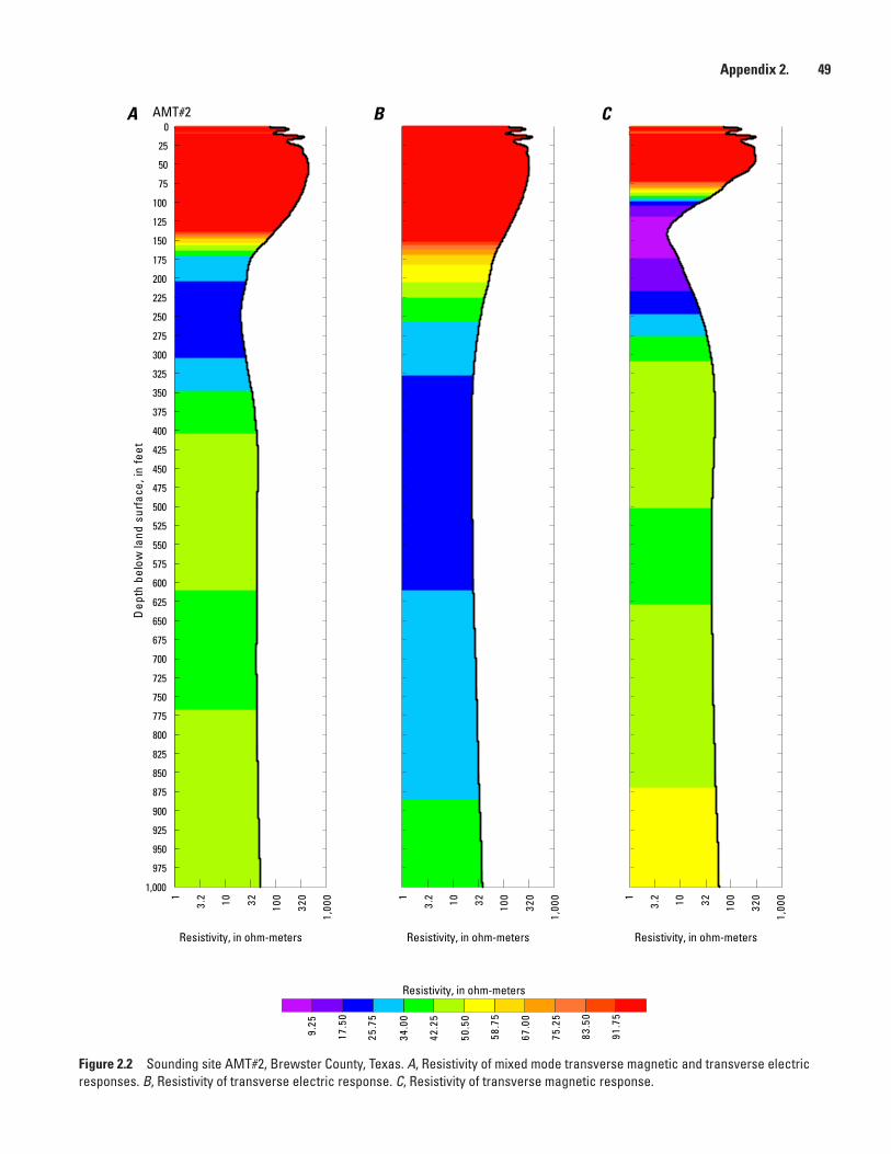
Appendix 2. 49
Figure 2.2 Sounding site AMT#2, Brewster County, Texas. A, Resistivity of mixed mode transverse magnetic and transverse electric responses. B, Resistivity of transverse electric response. C, Resistivity of transverse magnetic response.
3.2 10 32 100
320
1,00
01 1
3.2 10 32 100
320
1,00
0 1
3.2 10 32 100
320
1,00
0
25
50
75
100
125
150
175
200
225
250
275
300
325
350
375
400
425
450
475
500
525
550
575
600
625
650
675
700
725
750
775
800
825
850
875
900
925
950
975
1,000
AMT#20
Resistivity, in ohm-meters
Dep
th b
elow
land
sur
face
, in
feet
91.7
5
83.5
0
75.2
5
67.0
0
58.7
5
50.5
0
42.2
5
34.0
0
25.7
5
17.5
0
9.25
Resistivity, in ohm-meters
A B C
Resistivity, in ohm-meters Resistivity, in ohm-meters

50 Data Collection and Compilation for a Geodatabase, Pecos County Region, Texas, 1930–2011
Figure 2.3 Sounding site AMT#3, Jeff Davis County, Texas. A, Resistivity of mixed mode transverse magnetic and transverse electric responses. B, Resistivity of transverse electric response. C, Resistivity of transverse magnetic response.
11.
62.
5 46.
3 10 16 25 40 63 100 1
1.6
2.5 4
6.3 10 16 25 40 63 1
3.2 10 32 100
320
25
50
75
100
125
150
175
200
225
250
275
300
325
350
375
400
425
450
475
500
525
550
575
600
625
650
675
700
725
750
775
800
825
850
875
900
925
950
975
1,000
AMT#30
Resistivity, in ohm-meters
Dep
th b
elow
land
sur
face
, in
feet
91.7
5
83.5
0
75.2
5
67.0
0
58.7
5
50.5
0
42.2
5
34.0
0
25.7
5
17.5
0
9.25
Resistivity, in ohm-meters
A B C
Resistivity, in ohm-meters Resistivity, in ohm-meters

Appendix 2. 51
Figure 2.4 Sounding site AMT#4, Pecos County, Texas. A, Resistivity of mixed mode transverse magnetic and transverse electric responses. B, Resistivity of transverse electric response. C, Resistivity of transverse magnetic response.
1
3.2 10 32 100
320 1
3.2 10 32 100
320 1
3.2 10 32 100
320
25
50
75
100
125
150
175
200
225
250
275
300
325
350
375
400
425
450
475
500
525
550
575
600
625
650
675
700
725
750
775
800
825
850
875
900
925
950
975
1,000
AMT#40
Resistivity, in ohm-meters
Dep
th b
elow
land
sur
face
, in
feet
91.7
5
83.5
0
75.2
5
67.0
0
58.7
5
50.5
0
42.2
5
34.0
0
25.7
5
17.5
0
9.25
Resistivity, in ohm-meters
A B C
Resistivity, in ohm-meters Resistivity, in ohm-meters

52 Data Collection and Compilation for a Geodatabase, Pecos County Region, Texas, 1930–2011
Figure 2.5 Sounding site AMT#5, Pecos County, Texas. Resistivity of mixed mode transverse magnetic and transverse electric responses.
1
3.2 10 32 100
320
25
50
75
100
125
150
175
200
225
250
275
300
325
350
375
400
425
450
475
500
525
550
575
600
625
650
675
700
725
750
775
800
825
850
875
900
925
950
975
1,000
AMT#50
Resistivity, in ohm-meters
Dep
th b
elow
land
sur
face
, in
feet
91.7
5
83.5
0
75.2
5
67.0
0
58.7
5
50.5
0
42.2
5
34.0
0
25.7
5
17.5
0
9.25
Resistivity, in ohm-meters

Appendix 2. 53
Figure 2.6 Sounding site AMT#6, Pecos County, Texas. A, Resistivity of mixed mode transverse magnetic and transverse electric responses. B, Resistivity of transverse electric response. C, Resistivity of transverse magnetic response.
1
3.2 10 32 100
320
1,00
0 1
3.2 10 32 100
320 1
3.2 10 32 100
320
1,00
0
3,20
0
25
50
75
100
125
150
175
200
225
250
275
300
325
350
375
400
425
450
475
500
525
550
575
600
625
650
675
700
725
750
775
800
825
850
875
900
925
950
975
1,000
AMT#60
Resistivity, in ohm-meters
Dep
th b
elow
land
sur
face
, in
feet
91.7
5
83.5
0
75.2
5
67.0
0
58.7
5
50.5
0
42.2
5
34.0
0
25.7
5
17.5
0
9.25
Resistivity, in ohm-meters
A B C
Resistivity, in ohm-meters Resistivity, in ohm-meters

54 Data Collection and Compilation for a Geodatabase, Pecos County Region, Texas, 1930–2011
Figure 2.7 Sounding site AMT#7, Pecos County, Texas. A, Resistivity of mixed mode transverse magnetic and transverse electric responses. B, Resistivity of transverse electric response. C, Resistivity of transverse magnetic response.
1
3.2 10 32 100
320 1
3.2 10 32 100
320 1
3.2 10 32 100
320
25
50
75
100
125
150
175
200
225
250
275
300
325
350
375
400
425
450
475
500
525
550
575
600
625
650
675
700
725
750
775
800
825
850
875
900
925
950
975
1,000
AMT#70
Resistivity, in ohm-meters
Dep
th b
elow
land
sur
face
, in
feet
91.7
5
83.5
0
75.2
5
67.0
0
58.7
5
50.5
0
42.2
5
34.0
0
25.7
5
17.5
0
9.25
Resistivity, in ohm-meters
A B C
Resistivity, in ohm-meters Resistivity, in ohm-meters

Appendix 2. 55
Figure 2.8 Sounding site AMT#8, Pecos County, Texas. A, Resistivity of mixed mode transverse magnetic and transverse electric responses. B, Resistivity of transverse electric response. C, Resistivity of transverse magnetic response.
1
3.2 10 32 100
320 1
1.6
2.5 4
6.3 10 16 25 40 63 100 1
3.2 10 32 100
320
25
50
75
100
125
150
175
200
225
250
275
300
325
350
375
400
425
450
475
500
525
550
575
600
625
650
675
700
725
750
775
800
825
850
875
900
925
950
975
1,000
AMT#80
Resistivity, in ohm-meters
Dep
th b
elow
land
sur
face
, in
feet
91.7
5
83.5
0
75.2
5
67.0
0
58.7
5
50.5
0
42.2
5
34.0
0
25.7
5
17.5
0
9.25
Resistivity, in ohm-meters
A B C
Resistivity, in ohm-meters Resistivity, in ohm-meters

56 Data Collection and Compilation for a Geodatabase, Pecos County Region, Texas, 1930–2011
Figure 2.9 Sounding site AMT#9, Pecos County, Texas. Resistivity of mixed mode transverse magnetic and transverse electric responses.
11.
62.
5 46.
3 10 16 25 40 63
25
50
75
100
125
150
175
200
225
250
275
300
325
350
375
400
425
450
475
500
525
550
575
600
625
650
675
700
725
750
775
800
825
850
875
900
925
950
975
1,000
AMT#90
Resistivity, in ohm-meters
Dep
th b
elow
land
sur
face
, in
feet
91.7
5
83.5
0
75.2
5
67.0
0
58.7
5
50.5
0
42.2
5
34.0
0
25.7
5
17.5
0
9.25
Resistivity, in ohm-meters

Appendix 2. 57
Figure 2.10 Sounding site AMT#10, Pecos County, Texas. Resistivity of mixed mode transverse magnetic and transverse electric responses.
11.
62.
5 46.
3 10 16 25 40 63 100
25
50
75
100
125
150
175
200
225
250
275
300
325
350
375
400
425
450
475
500
525
550
575
600
625
650
675
700
725
750
775
800
825
850
875
900
925
950
975
1,000
AMT#100
Resistivity, in ohm-meters
Dep
th b
elow
land
sur
face
, in
feet
91.7
5
83.5
0
75.2
5
67.0
0
58.7
5
50.5
0
42.2
5
34.0
0
25.7
5
17.5
0
9.25
Resistivity, in ohm-meters

58 Data Collection and Compilation for a Geodatabase, Pecos County Region, Texas, 1930–2011
Figure 2.11 Sounding site AMT#11, Pecos County, Texas. A, Resistivity of mixed mode transverse magnetic and transverse electric responses. B, Resistivity of transverse electric response. C, Resistivity of transverse magnetic response.
1
3.2 10 32 100
320 1
3.2 10 32 100
320 1
3.2 10 32 100
320
25
50
75
100
125
150
175
200
225
250
275
300
325
350
375
400
425
450
475
500
525
550
575
600
625
650
675
700
725
750
775
800
825
850
875
900
925
950
975
1,000
AMT#110
Resistivity, in ohm-meters
Dep
th b
elow
land
sur
face
, in
feet
91.7
5
83.5
0
75.2
5
67.0
0
58.7
5
50.5
0
42.2
5
34.0
0
25.7
5
17.5
0
9.25
Resistivity, in ohm-meters
A B C
Resistivity, in ohm-meters Resistivity, in ohm-meters

Appendix 2. 59
Figure 2.12 Sounding site AMT#12, Reeves County, Texas. A, Resistivity of mixed mode transverse magnetic and transverse electric responses. B, Resistivity of transverse electric response. C, Resistivity of transverse magnetic response.
11.
62.
5 46.
3 10 16 25 40 63 100 1
1.6
2.5 4
6.3 10 16 25 40 63 100 1
3.2 10 32 100
320
25
50
75
100
125
150
175
200
225
250
275
300
325
350
375
400
425
450
475
500
525
550
575
600
625
650
675
700
725
750
775
800
825
850
875
900
925
950
975
1,000
AMT#120
Resistivity, in ohm-meters
Dep
th b
elow
land
sur
face
, in
feet
91.7
5
83.5
0
75.2
5
67.0
0
58.7
5
50.5
0
42.2
5
34.0
0
25.7
5
17.5
0
9.25
Resistivity, in ohm-meters
A B C
Resistivity, in ohm-meters Resistivity, in ohm-meters
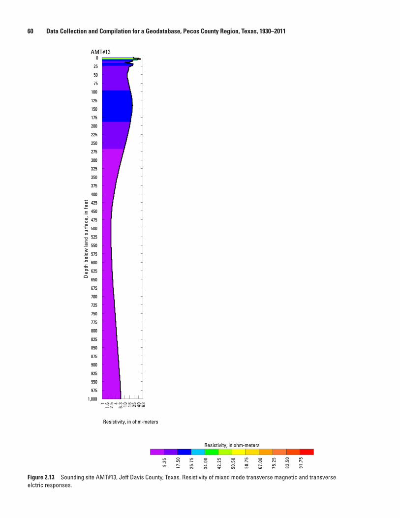
60 Data Collection and Compilation for a Geodatabase, Pecos County Region, Texas, 1930–2011
Figure 2.13 Sounding site AMT#13, Jeff Davis County, Texas. Resistivity of mixed mode transverse magnetic and transverse elctric responses.
11.
62.
5 46.
3 10 16 25 40 63
25
50
75
100
125
150
175
200
225
250
275
300
325
350
375
400
425
450
475
500
525
550
575
600
625
650
675
700
725
750
775
800
825
850
875
900
925
950
975
1,000
AMT#130
Resistivity, in ohm-meters
Dep
th b
elow
land
sur
face
, in
feet
91.7
5
83.5
0
75.2
5
67.0
0
58.7
5
50.5
0
42.2
5
34.0
0
25.7
5
17.5
0
9.25
Resistivity, in ohm-meters

Appendix 3. 61
Appendix 3. Digital Database Resources
Source: U.S. Environmental Protection Agency STORET ModernProcessing: Created sample table. Created unique site identifier by prefixing site_id assigned by sourcing agency with site_abv. Data Origination: Downloadable data- http://www.epa.gov/storet/Water-Quality Date Range: 8/15/1996 – 6/15/2011Number of sites: 7
Source: Middle Pecos Groundwater Conservation District Processing: Created unique site identifier by prefixing site_id assigned by sourcing agency with site_abv. Data Origination: File transfer protocol or other direct accessWater-Quality Date Range: no data availableNumber of Sites: 33
Source: Texas Commission on Environmental Quality , Surface Water Quality Information System Processing: Created sample table. Created unique site identifier by prefixing site_id assigned by sourcing agency with site_abv. Data Origination: File transfer protocol or other direct accessWater-Quality Date Range: 9/5/1968 – 8/24/1992Number of Sites: 13
Source: Texas Railroad CommissionProcessing: Created unique site identifier by prefixing site_id assigned by sourcing agency with site_abv. Data Origination: Downloadable data- http://www.rrc.state.tx.us/data/online/oilgasrecords.php (Texas Railroad Commission, 2011)Water-Quality Date Range: no data availableNumber of Sites: 6220
Source: Texas Water Development Board Groundwater Database (GWDB)Processing: Created sample table. Created unique site identifier by prefixing site_id assigned by sourcing agency with site_abv. Data Origination: Downloadable data- http://www.twdb.state.tx.us/groundwater/data/gwdbrpt.aspWater-Quality Date Range: 10/2/1930–4/30/2009Number of Sites: 1065
Source: U.S. Geological Survey, National Water Information SystemProcessing: Created unique site identifier by prefixing site_id assigned by sourcing agency with site_abv. Data Origination: File transfer protocol or other direct accessWater-Quality Date Range: 4/7/1932–6/23/2011Number of Sites: 81
Source: University of Texas System LandsProcessing: Created unique site identifier by prefixing site_id assigned by sourcing agency with site_abv. Data Origination: Downloadable data- http://www.utlands.utsystem.edu/WellSearchInfo.aspx (University of Texas System Lands, 2011)Water-Quality Date Range: no data available Number of Sites: 823

62 Data Collection and Compilation for a Geodatabase, Pecos County Region, Texas, 1930–2011
Source: City of Fort Stockton Well Locations (Domestic and Municipal)Processing: Created unique site identifier by prefixing site_id assigned by sourcing agency with site_abv. Data Origination: File transfer protocol or other direct accessWater-Quality Date Range: no data available Number of Sites: 281
Source: Daniel B. Stephens and Associates (Capitan Reef Study)Processing: Data compiled from digital media included previously published geologic formation picksData Origination: File transfer protocol or other direct accessWater-Quality Date Range: no data availableNumber of Sites: 153
Source: Texas Water Development Board Brackish Resources Aquifer Characterization SystemProcessing: Data compiled from digital media included previously published geologic formation picksData Origination: File transfer protocol or other direct access (Meyer and others, 2011) Water-Quality Date Range: no data availableNumber of Sites: 153

Appendix 4. 63
Appendix 4. Federal Geographic Data Committee-Compliant Metadata Record
Identification_Information Citation: Citation_Information: Originator: U.S. Geological Survey Publication_Date: 20111101 Title: Data Collection and Compilation for a Geodatabase, Pecos County Region, Texas, 1930–2011 Region, Texas, 2011 Geospatial_Data_Presentation_Form: vector digital data Description: Abstract: The U.S. Geological Survey, in cooperation with the Middle Pecos Groundwater Conservation
District, Pecos County, City of Fort Stockton, Brewster County, and Pecos County Water Control and Improvement District No. 1, developed a geodatabase of available groundwater, surface-water, water-quality, geophysical, and geology data for site locations in the Pecos County region, Texas. Data were compiled for an approximately 4,700 square mile area of the Pecos County region, Texas. The geodatabase, designed to warehouse field-collected geochemical and geophysical data, as well as digital database resources from the U.S. Geological Survey, Middle Pecos Groundwater Conservation District, Texas Water Development Board, Texas Commission on Environmental Quality, and numerous other State and local databases, contains 8,242 unique sampling locations. The geodatabase was used to combine these disparate database resources into a simple data model. Site locations are geospatially-enabled and stored in a geodatabase feature class for general mapping purposes and more rigorous spatial analysis. The sampling locations are related to the hydrogeologic information through the use of geodatabase relationship classes. The geodatabase relationship classes provide the ability to perform complex spatial and data-driven queries to explore data stored in the geodatabase .
Purpose: The purpose of this report is to provide information on data acquisition and geodatabase compilation of hydrogeologic data, Pecos County region, Texas. Groundwater, surface-water, water-quality, geophysical, and geologic information for more than 8,000 sampling locations were compiled from various digital data sources in the study area. Digital data sources were gathered from existing databases, previously published reports, and field-collected data.

64 Data Collection and Compilation for a Geodatabase, Pecos County Region, Texas, 1930–2011
Time_Period_of_Content: Time_Period_Information: Single_Date/Time: Calendar_Date: 2011 Currentness_Reference: 1930–2011 Status: Progress: On-going Maintenance_and_Update_Frequency: None Planned Spatial_Domain: Bounding_Coordinate: West_Bounding_Coordinate: -103.903888 East_Bounding_Coordinate: -101.816520 North_Bounding_Coordinate: 31.420552 South_Bounding_Coordinate: 30.356220 Keywords: Theme: Theme_Keyword: hydrogeology Theme_Keyword: groundwater Theme_Keyword: surface water Theme_Keyword: water quality Theme_Keyword: geology Place: Place_Keyword: Pecos County region Place_Keyword: Trans-Pecos Place_Keyword: Pecos County Place_Keyword: Reeves County Place_Keyword: Jeff Davis County Place_Keyword: Brewster County Place_Keyword: Terrell County Place_Keyword: Crane County Place_Keyword: Ward County Place_Keyword: Crockett County

Appendix 4. 65
Use_Constraints: These data are for informational purposes only. These data have not received Bureau approval and as such are provisional and subject to revision. The data are released on the condition that neither the U.S. Geological Survey, its cooperators, nor the U.S. Government may be held liable for any damages resulting from its authorized or unauthorized use. Although these data have been processed successfully on a computer system at the U.S. Geological Survey, no warranty expressed or implied is made regarding the accuracy or utility of the data on any other system or for general or scientific purposes, nor shall the act of distribution constitute any such warranty.
Native_Data_Set_Environment: Microsoft Microsoft Windows XP Version 5.1 (Build 2600) Service Pack 3; ESRI ArcGIS 10.0.0.2414
Data_Quality_Information: Lineage: Process_Step: Process_Description: Geographic locations of groundwater well sites, oil/gas well sites and surface- water sites were gathered from various Federal, State, and local databases. These data were compiled into a simplified feature class that maintains information related to: source agency, site identifier, unique identifier, site code (type), and site name. Process_Date: 20111101
Spatial_Data_Organization_Information: Direct_Spatial_Reference_Method: Vector Point_and_Vector_Object_Information: SDTS_Terms_Description: SDTS_Point_and_Vector_Object_Type: Entity point Point_and_Vector_Object_Count: 8242
Spatial_Reference_Information: Horizontal_Coordinate_System_Definition: Geographic: Latitude_Resolution: 0.000000 Longitude_Resolution: 0.000000 Geographic_Coordinate_Units: Decimal degrees

66 Data Collection and Compilation for a Geodatabase, Pecos County Region, Texas, 1930–2011
Geodetic_Model: Horizontal_Datum_Name: North American Datum of 1983 Ellipsoid_Name: Geodetic Reference System 80 Semi-major_Axis: 6378137.000000 Denominator_of_Flattening_Ratio: 298.257222
Entity_and_Attribute_Information: Detailed_Description: Entity_Type: Entity_Type_Label: sitefile Attribute: Attribute_Label: OBJECTID Attribute_Definition: Internal feature number. Attribute_Definition_Source: ESRI Attribute_Domain_Values: Unrepresentable_Domain: Sequential unique whole numbers that are automatically generated. Attribute: Attribute_Label: SHAPE Attribute_Definition: Feature geometry. Attribute_Definition_Source: ESRI Attribute_Domain_Values: Unrepresentable_Domain: Coordinates defining the features. Attribute: Attribute_Label: source_nm Attribute_Definition: Source name. Attribute: Attribute_Label: source_abv Attribute_Definition: Source abbreviation. Attribute: Attribute_Label: site_id Attribute_Definition: Native source identifier. Attribute: Attribute_Label: unique_id Attribute_Definition: Unique identifier is combination of source_abv and site_id fields. Attribute: Attribute_Label: site_cd Attribute_Definition: Site code.

Appendix 4. 67
Attribute: Attribute_Label: site_nm Attribute_Definition: Site name.
Distribution_Information: Resource_Description: Downloadable Data Metadata_Reference_Information: Metadata_Date: 20111101 Metadata_Contact: Contact_Information: Contact_Organization_Primary: Contact_Organization: U.S. Geological Survey Contact_Person: Public Information Officer Contact_Address: Address_Type: mailing and physical address Address: 1505 Ferguson Lane City: Austin State_or_Province: Texas Postal_Code: 78754 Country: USA Contact_Voice_Telephone: 512–927–3500 Contact_Facsimile_Telephone: 512–927–3590 Contact_Electronic_Mail_Address: [email protected] Metadata_Standard_Name: FGDC Content Standards for Digital Geospatial Metadata Metadata_Standard_Version: FGDC–STD–001–1998 Metadata_Time_Convention: local time Metadata_Extensions: Profile_Name: ESRI Metadata Profile
Prepared by the USGS Lafayette Publishing Service Center


Pearson and others—D
ata Collection and Compilation for a G
eodatabase, Pecos County Region, Texas, 1930–2011—Data Series 678
ISBN 978-1-4113-3373-4
9 7 8 1 4 1 1 3 3 3 7 3 4Printed on recycled paper