DATA AND SOFTWARE INTEROPERABILITY WITH GAMS: A USER PERSPECTIVE

Erwin Kalvelagenerwin@amsterdamoptimization.com

Amsterdam Optimization Modeling Group LLC

Modeling Languages

Specialized Modeling Languages (GAMS, AMPL,…) are very good in what they do Efficient, compact representation of a model

In a way that allows thinking about the complete model

And that allows and encourages experiments and reformulations

Through maintainable models

Especially when they become really big

Handle irregular and messy data well

API attraction: Σειρήν

Many new users are seducedto program against solver API’s

Familiar environment, no new funny language to learn

But for large, complex models this is really a step back

Even when using higher level modeling-fortified API’s

Modeling Environments

Environment Solver API Modeling API Modeling Language

GAMS, AMPL X

IBM ILOG Cplex API Concert OPL

MS Solver Foundation

Solver Level API SFS OML

GLPK API Mathprog

Malloc, Linker errors, Compiler versions, Library versions, Makefiles, Windows vs. Unix, Debuggers, …

Some programmers love:

But for others this is time taken away from modeling…

Also increased use of optimization in …

GAMS,AMPL,

…MATLAB

(Tomlab, Solver Interfaces)

R(Solver Interfaces,

Automatic Differentiation)

SAS(Improved OR

module)Excel

(MSF, Ilog, …)

Mathematica,Maple

(Numerical Routines)

Answer: Interoperability

Make GAMS more attractive for programmers by allowing to use external software

Make the user decide what to do in GAMS or in other environment

Make data exchange as easy as possible

Even for large data

Safety: this is a spot where lots of things can and will go wrong

Flexibility

Do not decide for user

Data manipulation can be done in GAMS or Excel

Computation can be done in GAMS or external software

Allow these decisions to be made depending on the situation

Skills

Available software

Suitability

E.g. Data handling

Office

Where to put functionality:In Date Source Environmentor Modeling SystemGAMS

AMPL

OMLThis has also to dowith proceduralvs declarative andwith data manipulationcapabilities

GDX in practice It really works

Binary, fast You can look at it

Limitations: Cannot add records or symbols Eg: combine two gdx files GDX is immutable

Not self contained wrt GAMS: Needs declarations

Zero vs non-existent GAMS interface $load is dangerous Compile time vs execution time Execution time limits (each call separate gdx, cannot add set

elements at execution time)

Example: USDA Farm database

Imports 3 MDB + 1 XLS file → 1 GDX file

± 5 million records (raw data)

File Size (bytes)

FARMLandWaterResourcesDraft.mdb 80,650,240

FARMResourcesProductionDraft.mdb 429,346,816

GTAP54-NonLandIntensive.mdb 303,616,000

FIPS2&FAOCountries.xls 29,184

farm.gdx 119,811,434

farm.gdx (compressed) 52,924,664

Good, compact way to distribute and reuse large data sets (input or output)

Aggregation easier in GAMS than in Access!

165 symbols

Example: USDA Reap Model

Combine data from different sources

Conversion mdb -> gdx$onecho > cmd.txtI=FeedGrainsData.mdbX=FeedGrainsData.gdx

q1=select commodity from tblCommoditiess1=commodity

q2=select attribute from tblAttributess2=attribute

q3=select period from tblTimePeriodss3=period

q4=select unit from tblUnitss4=unit

q5=select distinct(iif(isnull(isource),'blank',isource)) \from tblFG_update where \not isnull(year)

s5=isource

q6=select geo from tblgeographys6=geocode

q7=select commodity,attribute,unit,iif(isnull(isource),'blank',isource),geocode,year,period,value \from tblFG_update where \not isnull(year)

p7=feedgrains$offecho

$call mdb2gms @cmd.txt

Typical Problems

NULL’s

Duplicate records

Multivalued tables

More difficult processing:

Get latest available number

Difficult in SQL and in GAMS

Advantage of SQL: we canrepair a number of problemson the fly.

Data manipulation

Role of data manipulation in a modeling language

OML No data manipulation at all Do it in your data source environment (e.g. Excel)

AMPL More extensive data manipulation facilities Powerful if fits within declarative paradigm

GAMS Extensive use of data manipulation Procedural

Policy Evaluation Models

Often have serious data handling requirements

Aggregation/disaggregation

Estimation/Calibration

Simulation

Examples:

Loc= lines of code, comments excludedModel LOC LOC for equ’s

Polysys 22576 < 500

Impact2000 17284 0

IntegratedIW5 20177 < 500

Sparse Data: matrix multiplication

param N := 250;set I := {1..N};param A{i in I, j in I} := if (i=j) then 1;param B{i in I, j in I} := if (i=j) then 1;param C{i in I, j in I} := sum{k in I} A[i,k]*B[k,j];param s := sum{i in I, j in I} C[i,j];display s;end;

set i /1*250/;alias (i,j,k);parameter A(i,j),B(i,j),C(i,j);A(i,i) = 1;B(i,i) = 1;C(i,j) = sum(k, A(i,k)*B(k,j));scalar s;s = sum((i,j),C(i,j));display s;

Ampl

GAMS

Timings

0.1

1

10

100

150

200

250

gams-dense

gams-sparse

ampl-dense

ampl-sparse

glpk-dense

glpk-sparse

Solving Linear Equations

Solve Ax=b for x

Often not a good idea to calculate A-1

In GAMS we can solve by specifying Ax=b as equations

Inverse

If you really want the inverse of a matrix:

IAA 1

i.e. solve for A-1

Speed Up: Advanced Basis

We can provide advanced basis so the calculation takes 0 Simplex iterations

Inv.m(i,j) = 0; (var: basic)

Inverse.m(i,j) = 1; (equ: non-basic)

method=1 method=2 n=50 0.637 0.433 n=100 8.267 4.036 n=200 313.236 53.395

External Solver using GDX

execute_unload 'a.gdx',i,a;execute '=invert.exe a.gdx i a b.gdx pinva';parameter pinva(i,j);execute_load 'b.gdx',pinva;

i,A(i,j)

pinvA(i,j)

InvertGAMS

a.gdx

b.gdx

Test Matrix: Pei Matrix

1111

1111

1111

1111

method=1 method=2 method=3n=50 0.637 0.433 0.027n=100 8.267 4.036 0.055n=200 313.236 53.395 0.118

Other tools

Cholesky

Eigenvalue

Eigenvector

Max Likelihood Estimation

NLP solver can find optimal values: estimates

But to get covariances we need:

Hessian

Invert this Hessian

We can do this now in GAMS

Klunky, but at least we can now do this

GDX used several times

MLE Estimation Example* Data:* Number of days until the appearance of a carcinoma in 19* rats painted with carcinogen DMBA.

set i /i1*i19/;table data(i,*)

days censoredi1 143i2 164i3 188i4 188i5 190i6 192i7 206i8 209i9 213i10 216i11 220i12 227i13 230i14 234i15 246i16 265i17 304i18 216 1i19 244 1

;

set k(i) 'not censored';k(i)$(data(i,'censored')=0) = yes;

parameter x(i);x(i) = data(i,'days');

scalarsp 'number of observations'm 'number of uncensored observations'

;

p = card(i);m = card(k);

display p,m;

MLE Estimation

*-------------------------------------------------------------------------------* estimation*-------------------------------------------------------------------------------

scalar theta 'location parameter' /0/;

variablessigma 'scale parameter'c 'shape parameter'loglik 'log likelihood'

;

equation eloglike;

c.lo = 0.001;sigma.lo = 0.001;

eloglike.. loglik =e= m*log(c) - m*c*log(sigma)+ (c-1)*sum(k,log(x(k)-theta))- sum(i,((x(i)-theta)/sigma)**c);

model mle /eloglike/;solve mle maximizing loglik using nlp;

Get Hessian

*-------------------------------------------------------------------------------* get hessian*-------------------------------------------------------------------------------option nlp=convert;$onecho > convert.opthessian$offechomle.optfile=1;solve mle minimizing loglik using nlp;

** gams cannot add elements at runtime so we declare the necessary elements here*set dummy /e1,x1,x2/;

parameter h(*,*,*) '-hessian';execute_load "hessian.gdx",h;display h;

set j /sigma,c/;parameter h0(j,j);h0('sigma','sigma') = h('e1','x1','x1');h0('c','c') = h('e1','x2','x2');h0('sigma','c') = h('e1','x1','x2');h0('c','sigma') = h('e1','x1','x2');display h0;

Invert Hessian

*-------------------------------------------------------------------------------* invert hessian*-------------------------------------------------------------------------------

execute_unload "h.gdx",j,h0;execute "=invert.exe h.gdx j h0 invh.gdx invh";parameter invh(j,j);execute_load "invh.gdx",invh;display invh;

Normal Quantiles

*-------------------------------------------------------------------------------* quantile of normal distribution*-------------------------------------------------------------------------------

* find* p = 0.05* q = probit(1-p/2)

scalar prob /.05/;

* we don't have the inverse error function so we calculate it* using a small cns modelequations e;variables probit;e.. Errorf(probit) =e= 1-prob/2;model inverterrorf /e/;solve inverterrorf using cns;

display probit.l;

* verification:*> qnorm(0.975);*[1] 1.959964*>

Or just use 1.96

Finally: confidence intervals

*-------------------------------------------------------------------------------* calculate standard errors and confidence intervals*-------------------------------------------------------------------------------

parameter result(j,*);result('c','estimate') = c.l;result('sigma','estimate') = sigma.l;

result(j,'stderr') = sqrt(abs(invh(j,j)));

result(j,'conf lo') = result(j,'estimate') - probit.l*result(j,'stderr');result(j,'conf up') = result(j,'estimate') + probit.l*result(j,'stderr');

display result;

---- 168 PARAMETER result

estimate stderr conf lo conf up

sigma 234.319 9.646 215.413 253.224c 6.083 1.068 3.989 8.177

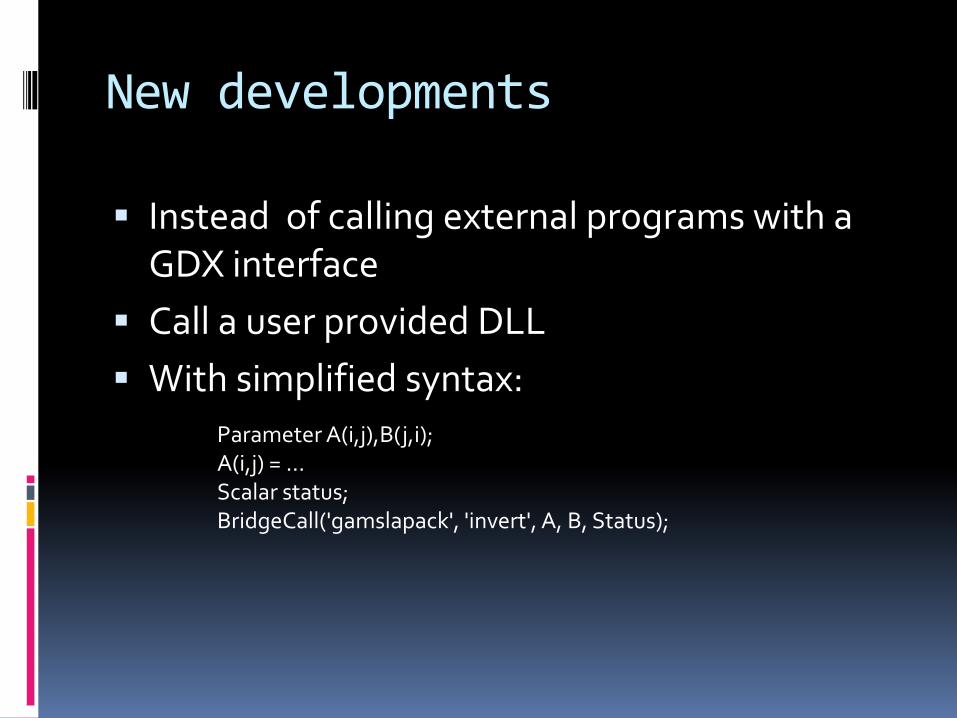
New developments

Instead of calling external programs with a GDX interface

Call a user provided DLL

With simplified syntax:

Parameter A(i,j),B(j,i);A(i,j) = …Scalar status;BridgeCall('gamslapack', 'invert', A, B, Status);

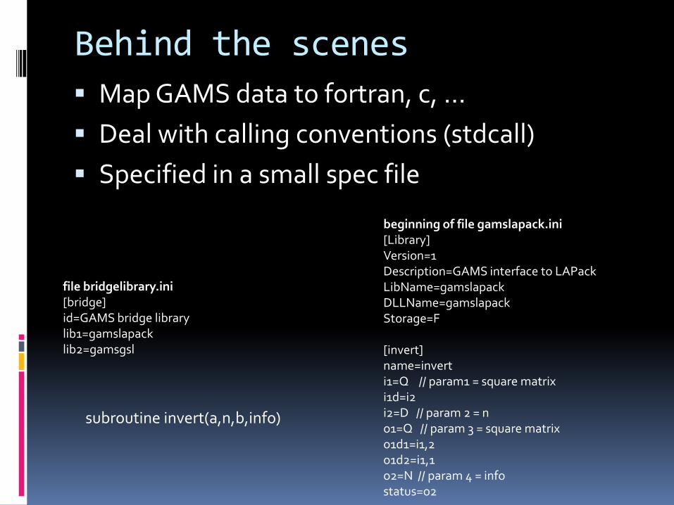
Behind the scenes

Map GAMS data to fortran, c, …

Deal with calling conventions (stdcall)

Specified in a small spec file

file bridgelibrary.ini[bridge]id=GAMS bridge librarylib1=gamslapacklib2=gamsgsl

beginning of file gamslapack.ini[Library]Version=1Description=GAMS interface to LAPackLibName=gamslapackDLLName=gamslapackStorage=F

[invert]name=inverti1=Q // param1 = square matrixi1d=i2 i2=D // param 2 = no1=Q // param 3 = square matrixo1d1=i1,2o1d2=i1,1o2=N // param 4 = infostatus=o2

subroutine invert(a,n,b,info)

Gets more exciting when…

We can parse subroutine headers

In libraries

And generate this automatically

This will open up access to Numerical, statistical libraries

Current tools as function (sql2gms, LS solver,…)

Etc.

Longer term: also for equations derivatives