2Data and Databases

2.1 Introduction

Multivariate data consist of multiple measurements, observations, or re-sponses obtained on a collection of selected variables. The types of variablesusually encountered often depend upon those who collect the data (the do-main experts), possibly together with some statistical colleagues; for it isthese people who actively decide which variables are of interest in study-ing a particular phenomenon. In other circumstances, data are collectedautomatically and routinely without a research direction in mind, usingsoftware that records every observation or transaction made regardless ofwhether it may be important or not.

Data are raw facts, which can be numerical values (e.g., age, height,weight), text strings (e.g., a name), curves (e.g., a longitudinal record re-garded as a single functional entity), or two-dimensional images (e.g., pho-tograph, map). When data sets are “small” in size, we find it convenientto store them in spreadsheets or as flat files (large rectangular arrays). Wecan then use any statistical software package to import such data for sub-sequent data analysis, graphics, and inference. As mentioned in Chapter 1,massive data sets are now sprouting up everywhere. Data of such size needto be stored and manipulated in special database systems.

A.J. Izenman, Modern Multivariate Statistical Techniques,doi: 10.1007/978-0-387-78189-1 2, 17c⃝ Springer Science+Business Media, LLC 2008

18 2. Data and Databases

2.2 Examples

We first describe some examples of the data sets to be encountered inthis book.

2.2.1 Example: DNA Microarray Data

The DNA (deoxyribonucleic acid) microarray has been described as “oneof the great unintended consequences of the Human Genome Project”(Baker, 2003). The main impact of this enormous scientific achievementis to provide us with large and highly structured microarray data sets fromwhich we can extract valuable genetic information. In particular, we wouldlike to know whether “gene expression” (the process by which genetic in-formation encoded in DNA is converted, first, into mRNA (messenger ri-bonucleic acid), and then into protein or any of several types of RNA) isany different for cancerous tissue as opposed to healthy tissue.

Microarray technology has enabled the expression levels of a huge num-ber of genes within a specific cell culture or tissue to be monitored si-multaneously and efficiently. This is important because differences in geneexpression determine differences in protein abundance, which, in turn, de-termine different cell functions. Although protein abundance is difficult todetermine, molecular biologists have discovered that gene expression canbe measured indirectly through microarray experiments.

Popular types of microarray technologies include cDNA microarrays (de-veloped at Stanford University) and high-density, synthetic, oligonucleotidemicroarrays (developed by Affymetrix, Inc., under the GeneChip R⃝ trade-mark). Both technologies use the idea of hybridizing a “target” (which isusually either a single-stranded DNA or RNA sequence, extracted from bio-logical tissue of interest) to a DNA “probe” (all or part of a single-strandedDNA sequence printed as “spots” onto a two-way grid of dimples in a glassor plastic microarray slide, where each spot corresponds to a specific gene).

The microarray slide is then exposed to a set of targets. Two biologi-cal mRNA samples, one obtained from cancerous tissue (the experimentalsample), the other from healthy tissue (the reference sample), are reverse-transcribed into cDNA (complementary DNA); then, the reference cDNAis labeled with a green fluorescent dye (e.g., Cy3) and the experimentalcDNA is labeled with a red fluorescent dye (e.g., Cy5). Fluorescence mea-surements are taken of each dye separately at each spot on the array. Highgene expression in the tissue sample yields large quantities of hybridizedcDNA, which means a high intensity value. Low intensity values derivefrom low gene expression.

The primary goal is to compare the intensity values, R and G, of thered and green channels, respectively, at each spot on the array. The most

2.2 Examples 19

popular statistic is the intensity log-ratio, M = log(R/G) = log(R)−log(G).Other such functions include the probe value, PV = log(R − G), and theaverage log-intensity, A = 1

2 (log R + log G). The logarithm in each case istaken to base 2 because intensity values are usually integers ranging from0 to 216 − 1.

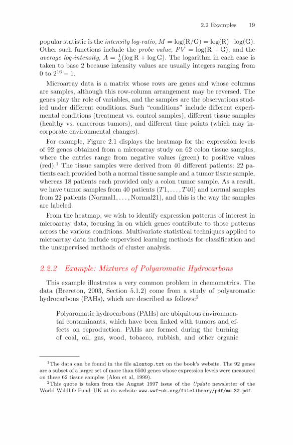
Microarray data is a matrix whose rows are genes and whose columnsare samples, although this row-column arrangement may be reversed. Thegenes play the role of variables, and the samples are the observations stud-ied under different conditions. Such “conditions” include different experi-mental conditions (treatment vs. control samples), different tissue samples(healthy vs. cancerous tumors), and different time points (which may in-corporate environmental changes).

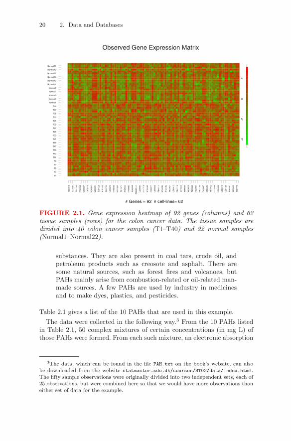
For example, Figure 2.1 displays the heatmap for the expression levelsof 92 genes obtained from a microarray study on 62 colon tissue samples,where the entries range from negative values (green) to positive values(red).1 The tissue samples were derived from 40 different patients: 22 pa-tients each provided both a normal tissue sample and a tumor tissue sample,whereas 18 patients each provided only a colon tumor sample. As a result,we have tumor samples from 40 patients (T1, . . . , T40) and normal samplesfrom 22 patients (Normal1, . . . ,Normal21), and this is the way the samplesare labeled.

From the heatmap, we wish to identify expression patterns of interest inmicroarray data, focusing in on which genes contribute to those patternsacross the various conditions. Multivariate statistical techniques applied tomicroarray data include supervised learning methods for classification andthe unsupervised methods of cluster analysis.

2.2.2 Example: Mixtures of Polyaromatic Hydrocarbons

This example illustrates a very common problem in chemometrics. Thedata (Brereton, 2003, Section 5.1.2) come from a study of polyaromatichydrocarbons (PAHs), which are described as follows:2

Polyaromatic hydrocarbons (PAHs) are ubiquitous environmen-tal contaminants, which have been linked with tumors and ef-fects on reproduction. PAHs are formed during the burningof coal, oil, gas, wood, tobacco, rubbish, and other organic

1The data can be found in the file alontop.txt on the book’s website. The 92 genesare a subset of a larger set of more than 6500 genes whose expression levels were measuredon these 62 tissue samples (Alon et al, 1999).

2This quote is taken from the August 1997 issue of the Update newsletter of theWorld Wildlife Fund–UK at its website www.wwf-uk.org/filelibrary/pdf/mu 32.pdf.

20 2. Data and Databases

T95

018

T71

025

T52

185

R78

934

M26

697

D63

874

M36

981

M63

391

T79

152

X15

183

Z50

753

U30

825

H40

560

M22

382

T51

571

X70

944

H40

095

Z49

269

Z49

269_

2

U29

092

H11

719

X12

466

R36

977

U09

564

R84

411

X74

295

X12

496

T62

947

U26

312

R64

115

L415

59

X86

693

X63

629

T83

368

R52

081

H87

135

D42

047

D00

596

X54

942

U17

899

H08

393

U32

519

U25

138

X56

597

X62

048

T60

778

T1

T3

T5

T7

T9

T11

T13

T15

T17

T19

T21

T23

T25

T27

T29

T31

T33

T35

T37

T39

Normal1

Normal3

Normal5

Normal7

Normal9

Normal11

Normal13

Normal15

Normal17

Normal19

Normal21

-4-2

02

Observed Gene Expression Matrix

# Genes = 92 # cell-lines= 62

FIGURE 2.1. Gene expression heatmap of 92 genes (columns) and 62tissue samples (rows) for the colon cancer data. The tissue samples aredivided into 40 colon cancer samples (T1–T40) and 22 normal samples(Normal1–Normal22).

substances. They are also present in coal tars, crude oil, andpetroleum products such as creosote and asphalt. There aresome natural sources, such as forest fires and volcanoes, butPAHs mainly arise from combustion-related or oil-related man-made sources. A few PAHs are used by industry in medicinesand to make dyes, plastics, and pesticides.

Table 2.1 gives a list of the 10 PAHs that are used in this example.The data were collected in the following way.3 From the 10 PAHs listed

in Table 2.1, 50 complex mixtures of certain concentrations (in mg L) ofthose PAHs were formed. From each such mixture, an electronic absorption

3The data, which can be found in the file PAH.txt on the book’s website, can alsobe downloaded from the website statmaster.sdu.dk/courses/ST02/data/index.html.The fifty sample observations were originally divided into two independent sets, each of25 observations, but were combined here so that we would have more observations thaneither set of data for the example.

2.2 Examples 21

TABLE 2.1. Ten polyaromatic hydrocarbon (PAH) compounds.

pyrene (Py), acenaphthene (Ace), anthracene (Anth), acenaphthylene (Acy),chrysene (Chry), benzanthracene (Benz), fluoranthene (Fluora), fluorene

(Fluore), naphthalene (Nap), phenanthracene (Phen)

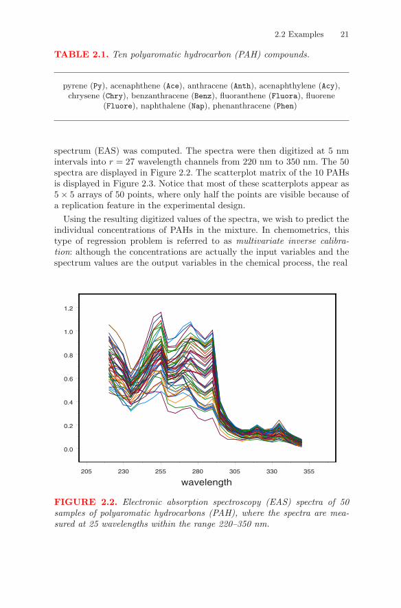
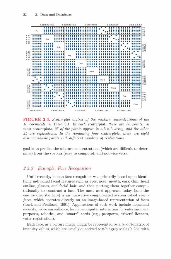
spectrum (EAS) was computed. The spectra were then digitized at 5 nmintervals into r = 27 wavelength channels from 220 nm to 350 nm. The 50spectra are displayed in Figure 2.2. The scatterplot matrix of the 10 PAHsis displayed in Figure 2.3. Notice that most of these scatterplots appear as5 × 5 arrays of 50 points, where only half the points are visible because ofa replication feature in the experimental design.

Using the resulting digitized values of the spectra, we wish to predict theindividual concentrations of PAHs in the mixture. In chemometrics, thistype of regression problem is referred to as multivariate inverse calibra-tion: although the concentrations are actually the input variables and thespectrum values are the output variables in the chemical process, the real

205 230 255 280 305 330 355

wavelength

0.0

0.2

0.4

0.6

0.8

1.0

1.2

FIGURE 2.2. Electronic absorption spectroscopy (EAS) spectra of 50samples of polyaromatic hydrocarbons (PAH), where the spectra are mea-sured at 25 wavelengths within the range 220–350 nm.

22 2. Data and Databases

Py

0.000.050.100.150.20

0.000.050.100.150.20

0.10.61.11.62.12.6

0.10.30.50.70.9

0.00.20.40.60.81.0

0.00.20.40.60.8

0.000.050.100.150.20

Ace

Anth

0.010.060.110.160.210.26

0.000.050.100.150.20

Acy

Chry

0.10.20.30.40.5

0.10.61.11.62.12.6

Benz

Fluora

0.000.050.100.150.20

0.10.30.50.70.9

Fluore

Nap

0.000.050.100.150.20

0.00.20.40.60.8

0.00.20.40.60.81.0

0.010.060.110.160.210.26

0.10.20.30.40.5

0.000.050.100.150.20

0.000.050.100.150.20

Phen

FIGURE 2.3. Scatterplot matrix of the mixture concentrations of the10 chemicals in Table 2.1. In each scatterplot, there are 50 points; inmost scatterplots, 25 of the points appear in a 5 × 5 array, and the other25 are replications. In the remaining four scatterplots, there are eightdistinguishable points with different numbers of replications.

goal is to predict the mixture concentrations (which are difficult to deter-mine) from the spectra (easy to compute), and not vice versa.

2.2.3 Example: Face Recognition

Until recently, human face recognition was primarily based upon identi-fying individual facial features such as eyes, nose, mouth, ears, chin, headoutline, glasses, and facial hair, and then putting them together compu-tationally to construct a face. The most used approach today (and theone we describe here) is an innovative computerized system called eigen-faces, which operates directly on an image-based representation of faces(Turk and Pentland, 1991). Applications of such work include homelandsecurity, video surveillance, human-computer interaction for entertainmentpurposes, robotics, and “smart” cards (e.g., passports, drivers’ licences,voter registration).

Each face, as a picture image, might be represented by a (c×d)-matrix ofintensity values, which are usually quantized to 8-bit gray scale (0–255, with

2.2 Examples 23

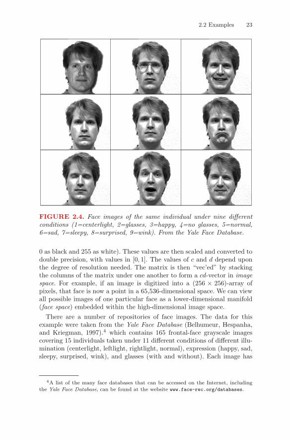
FIGURE 2.4. Face images of the same individual under nine differentconditions (1=centerlight, 2=glasses, 3=happy, 4=no glasses, 5=normal,6=sad, 7=sleepy, 8=surprised, 9=wink). From the Yale Face Database.

0 as black and 255 as white). These values are then scaled and converted todouble precision, with values in [0, 1]. The values of c and d depend uponthe degree of resolution needed. The matrix is then “vec’ed” by stackingthe columns of the matrix under one another to form a cd-vector in imagespace. For example, if an image is digitized into a (256 × 256)-array ofpixels, that face is now a point in a 65,536-dimensional space. We can viewall possible images of one particular face as a lower-dimensional manifold(face space) embedded within the high-dimensional image space.

There are a number of repositories of face images. The data for thisexample were taken from the Yale Face Database (Belhumeur, Hespanha,and Kriegman, 1997).4 which contains 165 frontal-face grayscale imagescovering 15 individuals taken under 11 different conditions of different illu-mination (centerlight, leftlight, rightlight, normal), expression (happy, sad,sleepy, surprised, wink), and glasses (with and without). Each image has

4A list of the many face databases that can be accessed on the Internet, includingthe Yale Face Database, can be found at the website www.face-rec.org/databases.

24 2. Data and Databases

size 320× 243, which then gets stacked into an r-vector, where r = 77, 760.Figure 2.4 shows the images of a single individual taken under 9 of those11 conditions. The problem is one of dimensionality reduction: what is thefewest number of variables necessary to identify these types of facial im-ages?

2.3 Databases

A database is a collection of persistent data, where by “persistent” wemean data that can be removed from the database only by an explicitrequest and not through an application’s side effect. The most popularformat for organizing data in a database is in the form of tables (also calleddata arrays or data matrices), each table having the form of a rectangulararray arranged into rows and columns, where a row represents the values ofall variables on a single multivariate observation (response, case, or record),and a column represents the values of a single variable for each observation.

In this book, a typical database table having n multivariate observationstaken on r variables will be represented by an (r × n)-matrix,

r×nX =

⎛

⎜⎜⎜⎝

x11 x12 · · · x1n

x21 x22 · · · x2n...

......

xr1 xr2 · · · xrn

⎞

⎟⎟⎟⎠, (2.1)

say, having r rows and n columns. In (2.1), xij represents the value in theith row (i = 1, 2, . . . , r) and jth column (j = 1, 2, . . . , n) of X . Althoughdatabase tables are set up to have the form of X τ , with variables as columnsand observations as rows, we will find it convenient in this book to set Xto be the transpose of the database table.

Databases exist for storing information. They are used for any of a num-ber of different reasons, including statistical analysis, retrieving informationfrom text-based documents (e.g., libraries, legislative records, case docketsin litigation proceedings), or obtaining administrative information (e.g.,personnel, sales, financial, and customer records) needed for managing anorganization. Databases can be of any size. Even small databases can bevery useful if accessed often. Setting up a large and complex database typi-cally involves a major financial committment on the part of an organization,and so the database has to remain useful over a long time period. Thus, weshould be able to extend a database as additional records become availableand to correct, delete, and update records as necessary.

2.3 Databases 25

2.3.1 Data Types

Databases usually consist of mixtures of different types of variables:

Indexing: These are usually names, tags, case numbers, or serial numbersthat identify a respondent or group of respondents. Their values mayindicate the location where a particular measurement was taken, orthe month or day of the year that an observation was made.

There are two special types of indexing variables:

1. A primary key is an indexing variable (or set of indexing vari-ables) that uniquely identifies each observation in a database(e.g., patient numbers, account numbers).

2. A foreign key is an indexing variable in a database where thatindexing variable is a primary key of a related database.

Binary: This is the simplest type of variable, having only two possibleresponses, such as YES or NO, SUCCESS or FAILURE, MALE orFEMALE, WHITE or NON-WHITE, FOR or AGAINST, SMOKERor NON-SMOKER, and so on. It is usually coded 0 or 1 for the twopossible responses and is often referred to as a dummy or indicatorvariable.

Boolean: A Boolean variable has the two responses TRUE or FALSE butmay also have the value UNKNOWN.

Nominal: This character-string data type is a more general version of abinary variable and has a fixed number of possible responses thatcannot be usefully ordered. These responses are typically coded al-phanumerically, and they usually represent disjoint classifications orcategories set up by the investigator. Examples include the geograph-ical location where data on other variables are collected, brand prefer-ence in a consumer survey, political party affiliation, and ethnic-racialidentification of respondent.

Ordinal: The possible responses for this character-string data type arelinearly ordered. An example is “excellent, good, fair, poor, bad, aw-ful” (or “strongly disagree” to “strongly agree”). Another exampleis bond ratings for debt issues, recorded as AA+, AA, AA-, A+, A,A-, B+, B, and B-. Such responses may be assigned scores or rank-ings. They are often coded on a “ranking scale” of 1–5 (or 1–10). Themain problem with these ranking scales is the implicit assumption ofequidistance of the assigned scores. Brand preferences can sometimesbe regarded as ordered.

26 2. Data and Databases

Integer: The response is usually a nonnegative whole number and is oftena count.

Continuous: This is a measured variable in which the continuity assump-tion depends upon a sufficient number of digits (and decimal places)being recorded. Continuous variables are specified as numeric or dec-imal in database systems, depending upon the precision required.

We note an important distinction between variables that are fixed andthose that are stochastic:

Fixed: The values of a fixed variable have deliberately been set in advance,as in a designed experiment, or are considered “causal” to the phe-nomenon in question; as a result, interest centers only on a specificgroup of responses. This category usually refers to indexing variablesbut can also include some of the above types.

Stochastic: The values of a stochastic variable can be considered as havingbeen chosen at random from a potential list (possibly, the real line ora portion of it) in some stochastic manner. In this sense, the valuesobtained are representative of the entire range of possible values ofthe variable in question.

We also need to distinguish between input and output variables:

Input variable: Also called a predictor or independent variable, typicallydenoted by X, and may be considered to be fixed (or preset or con-trolled) through a statistically designed experiment, or stochastic ifit can take on values that are observed but not controlled.

Output variable: Also called a response or dependent variable, typicallydenoted by Y , and which is stochastic and dependent upon the inputvariables.

Most of the methods described in this book are designed to elicit informa-tion concerning the extent to which the outputs depend upon the inputs.

2.3.2 Trends in Data Storage

As data collections become larger and larger, and areas of research thatwere once “data-poor” now become “data-rich,” it is how we store thosedata that is of great importance.

For the individual researcher working with a relatively simple database,data are stored locally on hard disks. We know that hard-disk storagecapacity is doubling annually (Kryder’s Law), and the trend toward tiny,

2.3 Databases 27

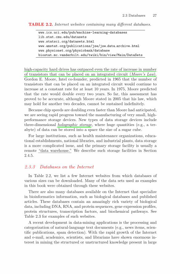
TABLE 2.2. Internet websites containing many different databases.

www.ics.uci.edu/pub/machine-learning-databaseslib.stat.cmu.edu/datasetswww.statsci.org/datasets.htmlwww.amstat.org/publications/jse/jse data archive.htmlwww.physionet.org/physiobank/databasebiostat.mc.vanderbilt.edu/twiki/bin/view/Main/DataSets

high-capacity hard drives has outpaced even the rate of increase in numberof transistors that can be placed on an integrated circuit (Moore’s Law).Gordon E. Moore, Intel co-founder, predicted in 1965 that the number oftransistors that can be placed on an integrated circuit would continue toincrease at a constant rate for at least 10 years. In 1975, Moore predictedthat the rate would double every two years. So far, this assessment hasproved to be accurate, although Moore stated in 2005 that his law, whichmay hold for another two decades, cannot be sustained indefinitely.

Because chip speeds are doubling even faster than Moore had anticipated,we are seeing rapid progress toward the manufacturing of very small, high-performance storage devices. New types of data storage devices includethree-dimensional holographic storage, where huge quantities (e.g., a ter-abyte) of data can be stored into a space the size of a sugar cube.

For large institutions, such as health maintenance organizations, educa-tional establishments, national libraries, and industrial plants, data storageis a more complicated issue, and the primary storage facility is usually aremote “data warehouse.” We describe such storage facilities in Section2.4.5.

2.3.3 Databases on the Internet

In Table 2.2, we list a few Internet websites from which databases ofvarious sizes can be downloaded. Many of the data sets used as examplesin this book were obtained through these websites.

There are also many databases available on the Internet that specializein bioinformatics information, such as biological databases and publishedarticles. These databases contain an amazingly rich variety of biologicaldata, including DNA, RNA, and protein sequences, gene expression profiles,protein structures, transcription factors, and biochemical pathways. SeeTable 2.3 for examples of such websites.

A recent development in data-mining applications is the processing andcategorization of natural-language text documents (e.g., news items, scien-tific publications, spam detection). With the rapid growth of the Internetand e-mail, academics, scientists, and librarians have shown enormous in-terest in mining the structured or unstructured knowledge present in large

28 2. Data and Databases

collections of text documents. To help those whose research interests liein analyzing text information, large databases (having more than 10,000features) of text documents are now available.

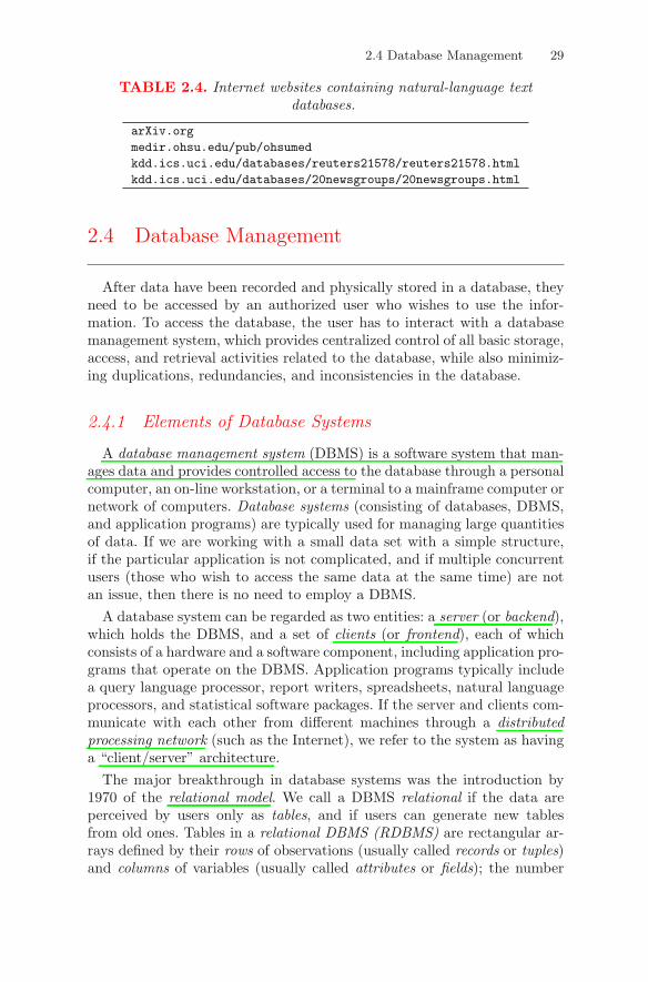
For example, Table 2.4 lists a number of text databases. Two of the mostpopular collections of documents come from Reuters, Ltd., which is theworld’s largest text and television news agency; the English-language col-lections Reuters-21578 containing 21,578 news items and RCV1 (ReutersCorpus Volume 1) (Lewis, Yang, Rose, and Li, 2004) containing 806,791news items are drawn from online databases. The 20 Newsgroups database(donated by Tom Mitchell) contains 20,000 messages taken from 20 Usenetnewsgroups. The OHSUMED text database (Hersh, Buckley, Leone, andHickam, 1994) from Ohio State University contains 348,566 references andabstracts derived from Medline, an on-line medical information database,for the period 1987–1991.

Computerized databases of scientific articles (e.g., arXiv, see Table 2.4)are assembled to (Shiffrin and Borner, 2004):

[I]dentify and organize research areas according to experts, insti-tutions, grants, publications, journals, citations, text, and figures;discover interconnections among these; establish the import ofresearch; reveal the export of research among fields; examinedynamic changes such as speed of growth and diversification;highlight economic factors in information production and dis-semination; find and map scientific and social networks; andidentify the impact of strategic and applied research funding bygovernment and other agencies.

A common element of text databases is the dimensionality of the data,which can run well into the thousands. This makes visualization especiallydifficult. Furthermore, because text documents are typically noisy, possiblyeven having differing formats, some automated preprocessing may be nec-essary in order to arrive at high-quality, clean data. The availability of textdatabases in which preprocessing has already been undertaken is provingto be an important development in database research.

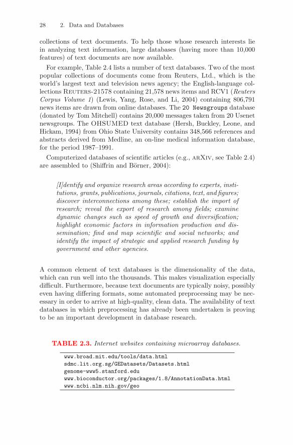
TABLE 2.3. Internet websites containing microarray databases.

www.broad.mit.edu/tools/data.htmlsdmc.lit.org.sg/GEDatasets/Datasets.htmlgenome-www5.stanford.eduwww.bioconductor.org/packages/1.8/AnnotationData.htmlwww.ncbi.nlm.nih.gov/geo

2.4 Database Management 29

TABLE 2.4. Internet websites containing natural-language textdatabases.

arXiv.orgmedir.ohsu.edu/pub/ohsumedkdd.ics.uci.edu/databases/reuters21578/reuters21578.htmlkdd.ics.uci.edu/databases/20newsgroups/20newsgroups.html

2.4 Database Management

After data have been recorded and physically stored in a database, theyneed to be accessed by an authorized user who wishes to use the infor-mation. To access the database, the user has to interact with a databasemanagement system, which provides centralized control of all basic storage,access, and retrieval activities related to the database, while also minimiz-ing duplications, redundancies, and inconsistencies in the database.

2.4.1 Elements of Database Systems

A database management system (DBMS) is a software system that man-ages data and provides controlled access to the database through a personalcomputer, an on-line workstation, or a terminal to a mainframe computer ornetwork of computers. Database systems (consisting of databases, DBMS,and application programs) are typically used for managing large quantitiesof data. If we are working with a small data set with a simple structure,if the particular application is not complicated, and if multiple concurrentusers (those who wish to access the same data at the same time) are notan issue, then there is no need to employ a DBMS.

A database system can be regarded as two entities: a server (or backend),which holds the DBMS, and a set of clients (or frontend), each of whichconsists of a hardware and a software component, including application pro-grams that operate on the DBMS. Application programs typically includea query language processor, report writers, spreadsheets, natural languageprocessors, and statistical software packages. If the server and clients com-municate with each other from different machines through a distributedprocessing network (such as the Internet), we refer to the system as havinga “client/server” architecture.

The major breakthrough in database systems was the introduction by1970 of the relational model. We call a DBMS relational if the data areperceived by users only as tables, and if users can generate new tablesfrom old ones. Tables in a relational DBMS (RDBMS) are rectangular ar-rays defined by their rows of observations (usually called records or tuples)and columns of variables (usually called attributes or fields); the number

30 2. Data and Databases

of tuples is called the cardinality, and the number of attributes is calledthe degree of the table. A RDBMS contains operators that enable users toextract specified rows (restrict) or specified columns (project) from atable and match up (join) information stored in different tables by check-ing for common entries in common columns. Also part of a DBMS is a datadictionary, which is a system database that stores information (metadata)about the database itself.

2.4.2 Structured Query Language (SQL)

Users communicate with a RDBMS through a declarative query language(or general interactive enquiry facility), which is typically one of the manyversions of SQL (Structured Query Language), usually pronounced “sequel”or “ess-cue-ell.” Created by IBM in the early 1970s and adopted as theindustry standard in 1986, there are now many different implementationsof SQL; no two are exactly the same, and each one is regarded as a dialect.In SQL, we can make a declarative statement that says, “From a givendatabase, extract data that satisfy certain conditions,” and the DBMS hasto determine how to do it.

SQL has two main sublanguages:

• a data definition language (DDL) is used primarily by database ad-ministrators to define data structures by creating a database object(such as a table) and altering or destroying a database object. It doesnot operate on data.

• a data manipulation language (DML) is an interactive system thatallows users to retrieve, delete, and update existing data from andadd new data to the database.

There is also a data control language (DCL), a security system used by thedatabase administrator, which controls the privileges granted to databaseusers.

Before creating a database consisting of multiple tables, it is advisable todo the following: give a unique name to each table; specify which columnseach table should contain and identify their data types; to each table, assigna primary key that uniquely identifies each row of the table; and have atleast one common column in each table in the database.

We can then build a working data set through the DDL by using SQLcreate table statements of the following form:

create table <table name> (<table elements>);

where <table name> specifies a name for the table and <table elements>is a list separated by commas that specifies column names, their data

2.4 Database Management 31

types, and any column constraints. The set of data types depends upon theSQL dialect; they include: char(c) (a column of characters where c givesthe maximum number of characters permitted in the column), integer,decimal(a, b) (where a is the total number of digits and b is the numberof decimal places), date (in DBMS-approved format), and logical (Trueor False). The column constraints include null (that column may haveempty row values) or not null (empty row values are not permitted inthat column), primary keys, and any foreign keys. A semicolon ends thestatement.

The DML includes such commands as select (allows users to retrievespecific database information), insert (adds new rows into an existingtable), update (modifies information contained within a table), and delete(removes rows from a table). DML commands can be quite complicated andmay include multiple expressions, clauses, predicates, or subqueries.

For example, the select statement (which supports restrict, project,and join operations, and is the most commonly used, but also most com-plicated SQL command) has the basic form

select <columns> from <table name> where <condition>;

where <columns> is a list of columns separated by commas. The selectcommand is used to gather certain attributes from a particular RDBMStable, but where the tuples (rows) that are to be retrieved from thosecolumns are limited to those that satisfy a given conditional Boolean searchexpression (i.e., True or False). One or more conditions may be joinedby and or or operators as in set theory (the and always precedes the oroperation). An asterisk may be used in place of the list of columns if allcolumns in the database are to be selected.

A primitive form of data analysis is included within the select statementthrough the use of five aggregate operators, sum, avg, max, min, and count,which provide the obvious column statistics over all rows that satisfy anystated conditions. For example, we can apply the command

select max(<column>) as max, min(<column>) as min from <tablename> where <condition>;

to find the maximum (saved as “max”) and minimum (saved as “min”) ofspecified columns. Column statistics that are not aggregates (e.g., medians)are not available in SQL.

The smaller RDBMSs that are available include Access (from MicrosoftCorp.), MySQL (open source), and mSQL (Hughes Technologies). These“lightweight” RDBMSs can support a few hundred simultaneous users andup to a gigabyte of data. All of the major statistical software packages thatoperate in a Windows environment can import data stored in certain ofthese smaller RDBMSs, especially Microsoft Access.

32 2. Data and Databases

We note that purists strongly object to SQL being thought of as a re-lational query language because, they argue, it sacrifices many of the fun-damental principles of the relational model in order to satisfy demands ofpracticality and performance. RDBMSs are slow in general and, becausethe dialects of SQL are different enough and are often incompatible witheach other, changing RDBMSs can be a nightmarish experience. Even so,SQL remains the most popular RDBMS query language.

2.4.3 OLTP Databases

A large organization is likely to maintain a DBMS that manages adomain-specific database for the automatic capture and storage of real-time business transactions. This type of database is essential for handlingan organization’s day-to-day operations. An on-line transaction processing(OLTP) system is a DBMS application that is specially designed for veryfast tracking of millions of small, simple transactions each day by a largenumber of concurrent users (tellers, cashiers, and clerks, who add, update,or delete a few records at a time in the database). Examples of OLTP data-bases include Internet-based travel reservations and airline seat bookings,automated teller machines (ATM) network transactions and point-of-saleterminals, transfers of electronic funds, stock trading records, credit cardtransactions and authorizations, and records of driving license holders.

These OLTP databases are dynamic in nature, changing almost contin-uously as transactions are automatically recorded by the system minute-by-minute. It is not unusual for an organization to employ several differentOLTP systems to carry out its various business functions (e.g., point-of-sale, inventory control, customer invoicing). Although OLTP systems areoptimized for processing huge numbers of short transactions, they are notconfigured for carrying out complex ad hoc and data analytic queries.

2.4.4 Integrating Distributed Databases

In certain situations, data may be distributed over many geographicallydispersed sites (nodes) connected by a communications network (usuallysome sort of local-area network or wide-area network, depending upon dis-tances involved). This is especially true for the healthcare industry. A hugeamount of information, for example, on hospital management practices maybe recorded from a number of different hospitals and consist of overlappingsets of variables and cases, all of which have to be combined (or integrated)into a single database for analysis.

Distributed databases also commonly occur in multicenter clinical trialsin the pharmaceutical industry, where centers include institutions, hospi-tals, and clinics, sometimes located in several countries. The number of

2.4 Database Management 33

total patients participating in such clinical trials rarely exceeds a few thou-sand, but there have been large-scale multicenter trials such as the ProstateCancer Prevention Trial (Baker, 2001), which is a chemoprevention trial inwhich 18,000 men aged 55 years and older were randomized to either dailyfinasteride or placebo tablets for 7 years and involved 222 sites in the UnitedStates.

Data integration is the process of merging data that originate from mul-tiple locations. When data are to be merged from different sources, severalproblems may arise:

• The data may be physically resident in computer files each of whichwas created using database software from different vendors.

• Different media formats may be used to store the information (e.g.,audio or video tapes or DVDs, CDs or hard disks, hardcopy question-naires, data downloaded over the Internet, medical images, scanneddocuments).

• The network of computer platforms that contain the data may beorganized using different operating systems.

• The geographical locations of those platforms may be local or remote.

• Parts of the data may be duplicated when collected from differentsources.

• Permission may need to be obtained from each source when deal-ing with sensitive data or security issues that will involve accessingpersonal, medical, business, or government records.

Faced with such potential inconsistencies, the information has to be inte-grated to become a consistent set of records for analysis.

2.4.5 Data Warehousing

An organization that needs to integrate multiple large OLTP databaseswill normally establish a single data warehouse for just that purpose. Theterm data warehouse was coined by W.H. Inmon to refer to a read-only,RDBMS running on a high-performance computer. The warehouse storeshistorical, detailed, and “scrubbed” data designed to be retrieved andqueried efficiently and interactively by users through a dialect of SQL.Although data are not updated in realtime, fresh data can be added assupplements at regular intervals.

The components of a data warehouse are

34 2. Data and Databases

DBMS: The publicly available RDBMSs that are almost mandatory fordata warehousing usage include Oracle (from Oracle Corp.), SQLServer (from Microsoft Corp.), Sybase (from Sybase Inc.), Post-greSQL (freeware), Informix (from Informix Software, Inc.), andDB2 (from IBM Corp.). These “heavyweight” DBMSs can handlethousands of simultaneous users and can access up to several ter-abytes of data.

Hardware: It is generally accepted that large-scale data warehouseapplications require either massively parallel-processing (MPP) orsymmetric multiprocessing (SMP) supercomputers. Which type ofhardware is installed depends upon many factors, including the com-plexity of the data and queries and the number of users that need toaccess the system.

• SMP architectures are often called “shared everything” becausethey share memory and resources to service more than a singleCPU, they run a single copy of the operating system, and theyshare a single copy of each application. SMP is reputed to bebetter for those data warehouses whose capacity ranges between50GB and 100GB.

• MPP architectures, on the other hand, are called “shared noth-ing”; they may have hundreds of CPUs in a single computer,each node of which is a self-contained computer with its ownCPU, disk, and memory, and nodes are connected by a high-speed bus or switch. The larger the data warehouse (with ca-pacity at least 200GB) and the more complex the queries, themore likely the organization will install an MPP server.

Such centralized data depositories typically contain huge quantities of in-formation taking up hundreds of gigabytes or terabytes of disk space. Smalldata warehouses, which store subsets of the central warehouse for use byspecialized groups or departments, are referred to as data marts.

More and more organizations that require a central data storage facilityare setting up their own data warehouses and data marts. For example,according to Monk (2000), the Foreign Trade Division of the U.S. CensusBureau processes 5 million records each month from the U.S. CustomsService on 18,000 import commodities and 9,000 export commodities thattravel between 250 countries and 50 regions within the United States. Theraw import-export data are extracted, “scrubbed,” and loaded into a datawarehouse having one terabyte of storage. Subsets of the data that focuson specific countries and commodities, together with two years of historicaldata, are then sent to a number of data marts for faster and more specificquerying.

2.4 Database Management 35

It has been reported that 90 percent of all Fortune 500 companies are cur-rently (or soon will be) engaged in some form of data warehousing activity.Corporations such as Federal Express, UPS, JC Penney, Office Depot, 3M,Ace Hardware, and Sears, Roebuck and Co. have installed data warehousesthat contain multi-terabytes of disk storage, and Wal-Mart and Kmart arealready at the 100 terabyte range. These retailers use their data warehousesto access comprehensive sales records (extracted from the scanners of cashregisters) and inventory records from thousands of stores worldwide.

Institutions of higher education now have data warehouses for informa-tion on their personnel, students, payroll, course enrollments and revenues,libraries, finance and purchasing, financial aid, alumni development, andcampus data. Healthcare facilities have data warehouses for storing uni-form billing data on hospital admissions and discharges, outpatient care,long-term care, individual patient records, physician licensing, certification,background, and specialties, operating and surgical profiles, financial data,CMS (Centers for Medicare and Medicaid Services) regulations, and nurs-ing homes, and that might soon include image data.

2.4.6 Decision Support Systems and OLAP

The failure of OLTP systems to deliver analytical support (e.g., statis-tical querying and data analysis) of RDBMSs caused a major crisis in thedatabase market until the concept of data warehouses each with its owndecision support system (DSS) emerged. In a client/server computing envi-ronment, decision support is carried out using on-line analytical processing(OLAP) software tools.

There are two primary architectures for OLAP systems, ROLAP (re-lational OLAP) and MOLAP (multidimensional OLAP); in both, multi-variate data are set up using a multidimensional model rather than thestandard model, which emphasizes data-as-tables. The two systems storedata differently, which in turn affects their performance characteristics andthe amounts of data that can be handled.

ROLAP operates on data stored in a RDBMS. Complex multipass SQLcommands can create various ad hoc multidimensional views of a two-dimensional data table (which slows down response times). ROLAPusers can access all types of transactional data, which are stored in100GB to multiple-terabyte data warehouses.

MOLAP operates on data stored in a specialized multidimensional DBMS.Variables are scaled categorically to allow transactional data to bepre-aggregated by all category combinations (which speeds up re-sponse times) and the results stored in the form of a “data cube”(a large, but sparse, multidimensional contingency table). MOLAPtools can handle up to 50GB of data stored in a data mart.

36 2. Data and Databases

OLAP users typically access multivariate databases without being awareexactly which system has been implemented. There are other OLAP sys-tems, including a hybrid version HOLAP.

The data analysis tools provided by a multidimensional OLAP systeminclude operators that can roll-up (aggregate further, producing marginals),drill-down (de-aggregate to search for possible irregularities in the aggre-gates), slice (condition on a single variable), and dice (condition on a par-ticular category) aggregated data in a multidimensional contingency table.Summary statistics that cannot be represented as aggregates (e.g., medi-ans, modes) and graphics that need raw data for display (e.g., scatterplots,time series plots) are generally omitted from MOLAP menus (Wilkinson,2005).

2.4.7 Statistical Packages and DBMSs

Some statistical analysis packages (e.g., SAS, SPSS) and Matlab canrun their complete libraries of statistical routines against their OLAP data-base servers.

A major effort is currently under way to provide a common interfacefor the S language (i.e., S-Plus and particularly R) to access the reallybig DBMSs so that sophisticated data analysis can be carried out in atransparent manner (i.e., DBMS and platform independent). Although atable in a RDBMS is very similar to the concept of data frame in R andS-Plus, there are many difficulties in building such interfaces.

The R package RODBC (written by Michael Lapsley and Brian Ripley,and available from CRAN) provides an R interface to DBMSs based uponthe Microsoft ODBC (Open Database Connectivity) standard. RODBC,which runs on both MS Windows and Unix/Linux, is able to copy an R dataframe to a table in a database (command: sqlSave), read a table from aDBMS into an R data frame (sqlFetch), submit an SQL query to an ODBCdatabase (sqlQuery), retrieve the results (sqlGetResults), and updatethe table where the rows already exist (sqlUpdate). RODBC works withOracle, MS Access, Sybase, DB2, MySQL, PostgreSQL, and SQLServer on MS Windows platforms and with MySQL, PostgreSQL, andOracle under Unix/Linux.

2.5 Data Quality Problems

Errors exist in all kinds of databases. Those that are easy to detect willmost likely be found at the data “cleaning” stage, whereas those errorsthat can be quite resistant to detection might only be discovered duringdata analysis. Data cleaning usually takes place as the data are received

2.5 Data Quality Problems 37

and before they are stored in read-only format in a data warehouse. Aconsistent and cleaned-up version of the data can then be made available.

2.5.1 Data Inconsistencies

Errors in compiling and editing the resulting database are common andactually occur with alarming frequency, especially in cases where the dataset is very large. When data from different sources are being connected,inconsistencies as to a person’s name (especially in cases where a namecan be spelled in several different ways) occur frequently, and matching (or“disambiguation”) has to take place before such records can be merged.One popular solution is to employ Soundex (sound-indexing) techniquesfor name matching.

To get an idea of how poor data quality can become, consider the prob-lem of estimating the extent of the undercount from census data collectedfor the 1990 U.S. census. Breiman (1994) identified a number of sourcesof error, including the following: Matching errors (incorrectly matchingrecords from two different files of people with differing names, ages, miss-ing gender or race identifiers, and different addresses), fabrications (thecreation of fictitious people by dishonest interviewers), census day addresserrors (incorrectly recording the location of a person’s residence on censusday), unreliable interviews (many of the interviews were rejected as beingunreliable), and incomplete data (a lack of specific information on certainmembers in the household). Most of the problems involving data fabri-cation, incomplete data, and unreliable interviews apparently occurred inareas that also had the highest estimated undercounts, such as the centralcities and minority areas.

Massive data sets are prone to mistakes, errors, distortions, and, in gen-eral, poor data quality, just as is any data set, but such defects occur hereon a far grander scale because of the size of the data set itself. When invalidproduct codes are entered for a product, they may easily be detected; whenvalid product codes, however, are entered for the wrong product, detectionbecomes more difficult. Customer codes may be entered inconsistently, es-pecially those for gender identification (M and F , as opposed to 1 and 2).Duplication of records entered into the database from multiple sources canalso be a problem. In these days of takeovers and buyouts, and mergers andacquisitions, what was once a code for a customer may now be a problem ifthe entity has since changed its description (e.g., Jenn-Air, Hoover, Norge,Magic Chef, etc., are all now part of Maytag Corp.). Any inconsistenciesin historical data may also be difficult to correct if those who knew theanswer are no longer with the company.

38 2. Data and Databases

2.5.2 Outliers

Outliers are values in the data that, for one reason or another, do notappear to fit the pattern of the other data values; visually, they are locatedfar away from the rest of the data. It is not unusual for outliers to bepresent in a data set.

Outliers can occur for many different reasons but should not be confusedwith gross errors. Gross errors are cases where “something went wrong”(Hampel, 2002); they include human errors (e.g., a numerical value recordedincorrectly) and mechanical errors (e.g., malfunctioning of a measuringinstrument or a laboratory instrument during analysis). The density ofgross errors depends upon the context and the quality of the data. Inmedical studies, gross error rates in excess of 10% have been quoted.

Univariate outliers are easy to detect when they indicate impossible (or“out of bounds”) values. More often, an outlier will be a value that is ex-treme, either too large or too small. For multivariate data, outlier detectionis more difficult. Low-dimensional visual displays of the data (such as his-tograms, boxplots, scatterplots) can encourage insight into the data andprovide at the same time a method for manually detecting some of themore obvious univariate or bivariate outliers.

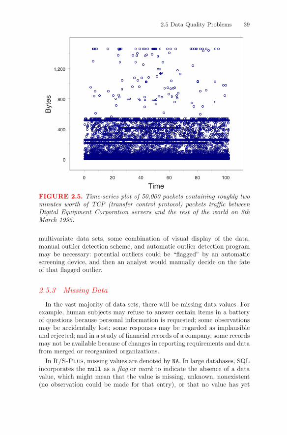
When we have a large data set, outliers may not be all that rare. Unlike adata set of 100 or so observations, where we may find two or three outliers,in a data set of 100,000, we should not be surprised to discover a largenumber (in some cases, hundreds, and maybe even thousands) of outliers.For example, Figure 2.5 shows a scatterplot of the size (in bytes) of eachof 50,000 packets5 containing roughly two minutes worth of TCP (transfercontrol protocol) packet traffic between Digital Equipment Corporationservers and the rest of the world on 8th March 1995 plotted against time.We see clear structure within the scatterplot: the vast majority of pointsoccur within the 0–512 bytes range, and a number of dense horizontal bandsoccur inside this range; these bands show that the vast majority of packetssent consist of either 0 bytes (37% of the total packets), which are usedonly to acknowledge data sent by the other side, or 512 bytes (29% of thetotal packets). There are 952 packets each having more than 512 bytes,of which 137 points are identified as outliers (with values greater than 1.5times IQR), including 61 points equal to the largest value, 1460 bytes.

To detect true multidimensional outliers, however, becomes a test ofstatistical ingenuity. A multivariate observation whose every componentvalue may appear indistinguishable from the rest may yet be regardedas an outlier when all components are treated simultaneously. In large

5See www.amstat.org/publications/jse/datasets/packetdata.txt.

2.5 Data Quality Problems 39

0 20 40 60 80 100

Time

0

400

800

1,200

Byt

es

FIGURE 2.5. Time-series plot of 50,000 packets containing roughly twominutes worth of TCP (transfer control protocol) packets traffic betweenDigital Equipment Corporation servers and the rest of the world on 8thMarch 1995.

multivariate data sets, some combination of visual display of the data,manual outlier detection scheme, and automatic outlier detection programmay be necessary: potential outliers could be “flagged” by an automaticscreening device, and then an analyst would manually decide on the fateof that flagged outlier.

2.5.3 Missing Data

In the vast majority of data sets, there will be missing data values. Forexample, human subjects may refuse to answer certain items in a batteryof questions because personal information is requested; some observationsmay be accidentally lost; some responses may be regarded as implausibleand rejected; and in a study of financial records of a company, some recordsmay not be available because of changes in reporting requirements and datafrom merged or reorganized organizations.

In R/S-Plus, missing values are denoted by NA. In large databases, SQLincorporates the null as a flag or mark to indicate the absence of a datavalue, which might mean that the value is missing, unknown, nonexistent(no observation could be made for that entry), or that no value has yet

40 2. Data and Databases

been assigned. A null is not equivalent to a zero value or to a text stringfilled with spaces. Sometimes, missing values are replaced by zeroes, othertimes by estimates of what they should be based on the rest of the data.

One popular method deletes those observations that contain missing dataand analyzes only those cases that are observed in their entirety (oftencalled complete-case analysis or listwise-deletion method). Such a complete-case analysis may be satisfactory if the proportion of deleted observationsis small relative to the size of the entire data set and if the mechanism thatleads to the missing data is independent of the variables in question —an assumption referred to by Donald Rubin as missing at random (MAR)or missing completely at random (MCAR) depending upon the exact na-ture of the missing-data mechanism (Little and Rubin, 1987). Any deletedobservations may be used to help justify the MCAR assumption.

If the missing data constitute a sizeable proportion of the entire dataset, then complete-case methods will not work. Single imputation has beenused to impute (or “fill in”) an estimated value for each missing obser-vation and then analyze the amended data set as if there had been nomissing values in the first place. Such procedures include hot-deck impu-tation, where a missing value is imputed by substituting a value from asimilar but complete record in the same data set; mean imputation, wherethe singly imputed value is just the mean of all the completely recordedvalues for that variable; and regression imputation, which uses the valuepredicted by a regression on the completely recorded data. Because sam-pling variability due to single imputation cannot be incorporated into theanalysis as an additional source of variation, the standard errors of modelestimates tend to be underestimated.

Since the late 1970s, Rubin and his colleagues have introduced a num-ber of sophisticated algorithmic methods for dealing with incomplete datasituations. One approach, the EM algorithm (Dempster, Laird, and Rubin,1977; Little and Rubin, 1987), which alternates between an expectation (E)step and a maximization (M) step, is used to compute maximum-likelihoodestimates of model parameters, where missing data are modeled as unob-served latent variables. We shall describe applications of the EM algorithmin more detail in later chapters of this book. A different approach, multipleimputation (Rubin, 1987), fills in the missing values m > 1 times, wherethe imputed values are generated each time from a distribution that maybe different for each missing value; this creates m different data sets, whichare analyzed separately, and then the m results are combined to estimatemodel parameters, standard errors, and confidence intervals.

2.5.4 More Variables than Observations

Many statistical computer packages do not allow the number of inputvariables, r, to exceed the number of observations, n, because, then, certain

2.6 The Curse of Dimensionality 41

matrices, such as the (r × r) covariance matrix, would have less than fullrank, would be singular, and, hence, uninvertible. Yet, we should not besurprised when r > n. In fact, this situation occurs quite routinely incertain applications, and in such instances, r can be much greater than n.Typical examples include:

Satellite images When producing maps, remotely sensed image data aregathered from many sources, including satellite and aircraft scanners,where a few observations (usually fewer than 10 spectral bands) aremeasured at more than 100,000 wavelengths over a grid of pixels.

Chemometrics For determining concentrations in certain chemical com-pounds, calibration studies often need to analyze intensity measure-ments on a very large number (500–1,000 or more) of different spectralwavelengths using a small number of standard chemical samples.

Gene expression data Current microarray methods for studying humanmalignancies, such as tumors, simultaneously monitor expression lev-els of very large numbers of genes (5,000–10,000 or more) on relativelysmall numbers (fewer than 100) of tumor samples.

When r > n, one way of dealing with this problem is to analyze the dataon each variable separately. However, this suggestion does not take accountof correlations between the variables. Researchers have recently providednew statistical techniques that are not sensitive to the r > n issue. We willaddress this situation in various sections of this book.

2.6 The Curse of Dimensionality

The term “curse of dimensionality” (Bellman, 1961) originally describedhow difficult it was to perform high-dimensional numerical integration. Thisled to the more general use of the term to describe the difficulty of dealingwith statistical problems in high dimensions. Some implications include:

1. We can never have enough data to cover every part of high-dimensionalinput space to learn which part of the space is important to a relationshipand which is not.

To see this, divide the axis of each of r input variables into K uniform in-tervals (or “bins”), so that the value of an input variable is approximated bythe bin into which it falls. Such a partition divides the entire r-dimensionalinput space into Kr “hypercubes,” where K is chosen so that each hy-percube contains at least one point in the input space. Given a specifichypercube in input space, an output value y0 corresponding to a new inputpoint in the hypercube can be approximated by computing some function

42 2. Data and Databases

(e.g., the average value) of the y values that correspond to all the inputpoints falling in that hypercube. Increasing K reduces the sizes of the hy-percubes while increasing the precision of the approximation. However, atthe same time, the number of hypercubes increases exponentially. If therehas to be at least one input point in each hypercube, then the number ofsuch points needed to cover all of r-space must also increase exponentiallyas r increases. In practice, we have a limited number of observations, withthe result that the data are very sparsely spread around high-dimensionalspace.

2. As the number of dimensions grows larger, almost all the volumeinside a hypercubic region of input space lies closer to the boundary orsurface of the hypercube rather than near the center.

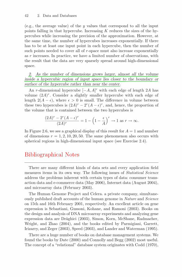
An r-dimensional hypercube [−A,A]r with each edge of length 2A hasvolume (2A)r. Consider a slightly smaller hypercube with each edge oflength 2(A − ϵ), where ϵ > 0 is small. The difference in volume betweenthese two hypercubes is (2A)r − 2r(A − ϵ)r, and, hence, the proportion ofthe volume that is contained between the two hypercubes is

(2A)r − 2r(A − ϵ)r

(2A)r= 1 −

(1 − ϵ

A

)r→ 1 as r → ∞.

In Figure 2.6, we see a graphical display of this result for A = 1 and numberof dimensions r = 1, 2, 10, 20, 50. The same phenomenon also occurs withspherical regions in high-dimensional input space (see Exercise 2.4).

Bibliographical Notes

There are many different kinds of data sets and every application fieldmeasures items in its own way. The following issues of Statistical Scienceaddress the problems inherent with certain types of data: consumer trans-action data and e-commerce data (May 2006), Internet data (August 2004),and microarray data (February 2003).

The Human Genome Project and Celera. a private company, simultane-ously published draft accounts of the human genome in Nature and Scienceon 15th and 16th February 2001, respectively. An excellent article on geneexpression is Sebastiani, Gussoni, Kohane, and Ramoni (2003). Books onthe design and analysis of DNA microarray experiments and analyzing geneexpression data are Draghici (2003), Simon, Korn, McShane, Radmacher,Wright, and Zhao (2004), and the books edited by Parmigiani, Garrett,Irizarry, and Zeger (2003), Speed (2003), and Lander and Waterman (1995).

There are a huge number of books on database management systems. Wefound the books by Date (2000) and Connolly and Begg (2002) most useful.The concept of a “relational” database system originates with Codd (1970),

2.6 The Curse of Dimensionality 43

0.1 0.3 0.5 0.7 0.9

e

0.0

0.2

0.4

0.6

0.8

1.0P

ropo

rtio

n of

Vol

ume

r = 1

r = 2

r = 10

r = 20

r = 50

FIGURE 2.6. Graphs of the proportion of the total volume contained be-tween two hypercubes, one of edge length 2 and the other of edge length2 − e for different numbers of dimensions r. As the number of dimensionsincreases, almost all the volume becomes closer to the surface of the hyper-cube.

who received the 1981 ACM Turing Award for his work in the area. An ex-cellent survey of the development and maintenance of biological databasesand microarray repositories is given by Valdivia-Granda and Dwan (2006).

Books on missing data include Little and Rubin (1987) and Schafer(1997). A book on the EM algorithm is McLachlan and Krishnan (1997).For multiple imputation, see the book by Rubin (1987). Books on out-lier detection include Rousseeuw and Leroy (1987) and Barnett and Lewis(1994).

Exercises

2.1 In a statistical application of your choice, what does a missing valuemean? What are the traditional methods of imputing missing values insuch an application?

2.2 In sample surveys, such as opinion polls, telephone surveys, and ques-tionnaire surveys, nonresponse is a common occurrence. How would youdesign such a survey so as to minimize nonresponse?

2.3 Discuss the differences between single and multiple imputation forimputing missing data.

44 2. Data and Databases

2.4 The volume of an r-dimensional sphere with radius A is given byvolr(A) = SrAr/r, where Sr = 2πr/2/Γ(r/2) is the surface area of theunit sphere in r dimensions, Γ(x) =

∫ ∞0 tx−1e−tdt = (x − 1)!, 1x > 0,

is the gamma function, Γ(x + 1) = xΓ(x), and Γ(1/2) = π1/2. Find theappropriate spherical volumes for two and three dimensions. Using a similarlimiting argument as in (2) of Section 2.6, show that as the dimensionalityincreases, almost all the volume inside the sphere tends to be concentratedalong a “thin shell” closer to the surface of the sphere than to the center.

2.5 Consider a hypercube of dimension r and sides of length 2A andinscribe in it an r-dimensional sphere of radius A. Find the proportion ofthe volume of the hypercube that is inside the hypersphere, and show thatthe proportion tends to 0 as the dimensionality r increases. In other words,show that all the density sits in the corners of the hypercube.

2.6 What are the advantages and disadvantages of database systems, andwhen would you find such a system useful for data analysis?

2.7 Find a commercial SQL product and discuss the various options thatare available for the create table statement of that product.

2.8 Find a DBMS and investigate whether that system keeps track ofdatabase statistics. Which statistics does it maintain, how does it do that,and how does it update those statistics?

2.9 What are the advantages and disadvantages of distributed databasesystems?

2.10 (Fairley, Izenman, and Crunk, 2001) You are hired to carry out asurvey of damage to the bricks of the walls of a residential complex con-sisting of five buildings, each having 5, 6, or 7 stories. The type of damageof interest is called spalling and refers to deterioration of the surface of thebrick, usually caused by freeze-thaw weather conditions. Spalling appearsto be high at the top stories and low at the ground. The walls consist ofthree-quarter million bricks. You take a photographic survey of all the wallsof the complex and count the number of bricks in the photographs that arespalled. However, the photographs show that some portions of the wallsare obscured by bushes, trees, pipes, vehicles, etc. So, the photographs arenot a complete record of brick damage in the complex. Discuss how wouldyou estimate the spall rate (spalls per 1,000 bricks) for the entire complex.What would you do about the missing data in your estimation procedure?

2.11 Read about MAR (missing at random) and MCAR (missing com-pletely at random) and discuss their differences and implications for im-puting missing data.