Report EUR 27358 EN

Dario Simonetti Andrea Marelli Hugh Eva

20 1 5

1

European Commission

Joint Research Centre

Institute for Environment and Sustainability

Contact information

Dario Simonetti

Address: Joint Research Centre, Via Enrico Fermi 2749, TP 260, 21027 Ispra (VA), Italy

E-mail: dario.simonetti@jrc.ec.europa.eu

Tel.: +39 0332 78 3871

JRC Science Hub

https://ec.europa.eu/jrc

Legal Notice

This publication is a Technical Report by the Joint Research Centre, the European Commission’s in-house

science service.

It aims to provide evidence-based scientific support to the European policy-making process. The scientific output

expressed does not imply a policy position of the European Commission. Neither the European Commission nor

any person acting on behalf of the Commission is responsible for the use which might be made of this publication.

All images © European Union 2015

JRC96789

EUR 27358 EN

ISBN 978-92-79-50115-9

ISSN 1831-9424

doi:10.2788/143497

Luxembourg: Publications Office of the European Union, 2015

© European Union, 2015

Reproduction is authorised provided the source is acknowledged.

Abstract

Did you ever try to produce a reliable land cover map from Earth Observation data? How many steps are involved

and how many different tools do you need? Did you succeed in a reasonable amount of time?

IMPACT toolbox offers a combination of elements of remote sensing, photo interpretation and processing

technologies in a portable and stand-alone GIS environment, allowing non ITC users to easily accomplish all

necessary pre-processing steps while giving a fast and user-friendly environment for visual editing and map

validation.

2

Table of Contents .................................................................................................................................................... 1

1. Overview ............................................................................................................................ 3

2. Introduction ........................................................................................................................ 4

3. Structure.............................................................................................................................. 4

4. Main Panel .......................................................................................................................... 6

5. Processing Modules ............................................................................................................ 8

5.1 Processing Modules: Evergreen Forest Normalization ............................................ 24

6. Map Validation Panel ....................................................................................................... 25

7. Ground Truth Collection Panel ......................................................................................... 28

8. 3 Epochs Map Validation Panel ....................................................................................... 31

9. Settings Panel ................................................................................................................... 35

10. IMPACT: well-known issues ........................................................................................ 36

11. IMPACT: future developments …................................................................................ 37

12. Version .......................................................................................................................... 38

13. License .......................................................................................................................... 38

14. Copyright ...................................................................................................................... 38

Acknowledgments.................................................................................................................... 39

Annex 1: Image segmentation ................................................................................................. 40

This document version 1.0 dated 10/2015 is referring to the IMPACT toolbox 1.0 beta.

Please check the last version on http://forobs.jrc.ec.europa.eu/products/software

3

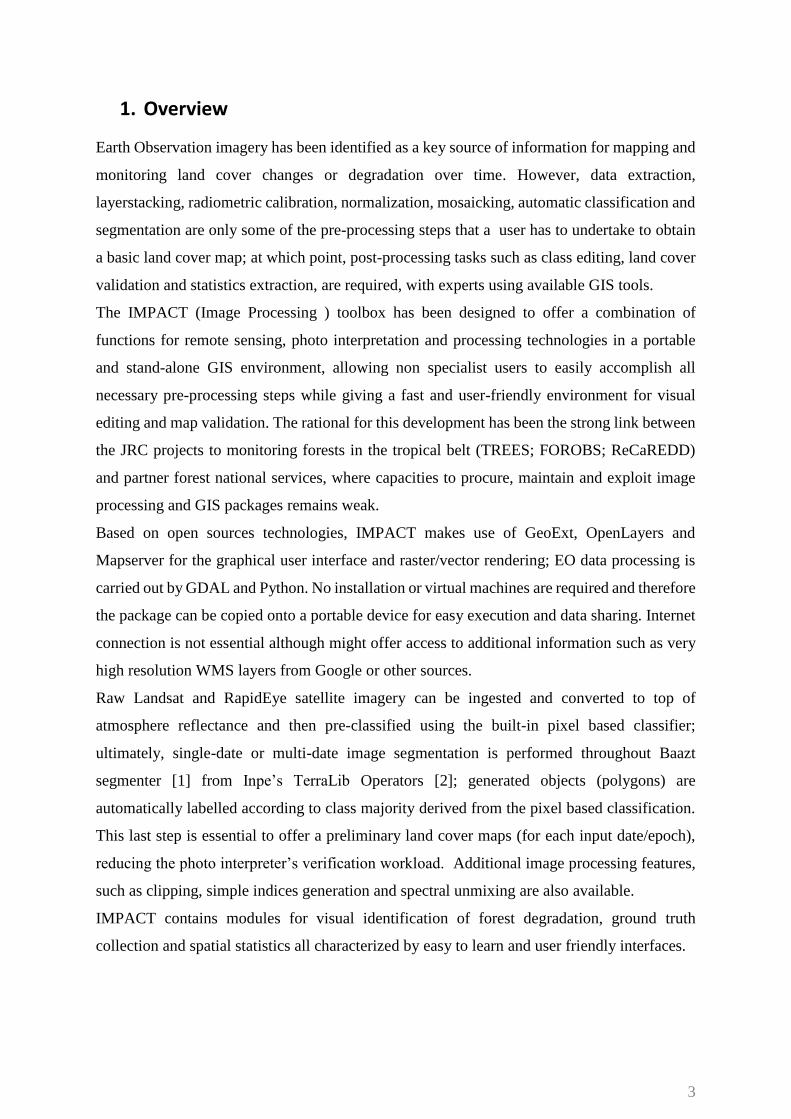
1. Overview

Earth Observation imagery has been identified as a key source of information for mapping and

monitoring land cover changes or degradation over time. However, data extraction,

layerstacking, radiometric calibration, normalization, mosaicking, automatic classification and

segmentation are only some of the pre-processing steps that a user has to undertake to obtain

a basic land cover map; at which point, post-processing tasks such as class editing, land cover

validation and statistics extraction, are required, with experts using available GIS tools.

The IMPACT (Image Processing ) toolbox has been designed to offer a combination of

functions for remote sensing, photo interpretation and processing technologies in a portable

and stand-alone GIS environment, allowing non specialist users to easily accomplish all

necessary pre-processing steps while giving a fast and user-friendly environment for visual

editing and map validation. The rational for this development has been the strong link between

the JRC projects to monitoring forests in the tropical belt (TREES; FOROBS; ReCaREDD)

and partner forest national services, where capacities to procure, maintain and exploit image

processing and GIS packages remains weak.

Based on open sources technologies, IMPACT makes use of GeoExt, OpenLayers and

Mapserver for the graphical user interface and raster/vector rendering; EO data processing is

carried out by GDAL and Python. No installation or virtual machines are required and therefore

the package can be copied onto a portable device for easy execution and data sharing. Internet

connection is not essential although might offer access to additional information such as very

high resolution WMS layers from Google or other sources.

Raw Landsat and RapidEye satellite imagery can be ingested and converted to top of

atmosphere reflectance and then pre-classified using the built-in pixel based classifier;

ultimately, single-date or multi-date image segmentation is performed throughout Baazt

segmenter [1] from Inpe’s TerraLib Operators [2]; generated objects (polygons) are

automatically labelled according to class majority derived from the pixel based classification.

This last step is essential to offer a preliminary land cover maps (for each input date/epoch),

reducing the photo interpreter’s verification workload. Additional image processing features,

such as clipping, simple indices generation and spectral unmixing are also available.

IMPACT contains modules for visual identification of forest degradation, ground truth

collection and spatial statistics all characterized by easy to learn and user friendly interfaces.

4

2. Introduction

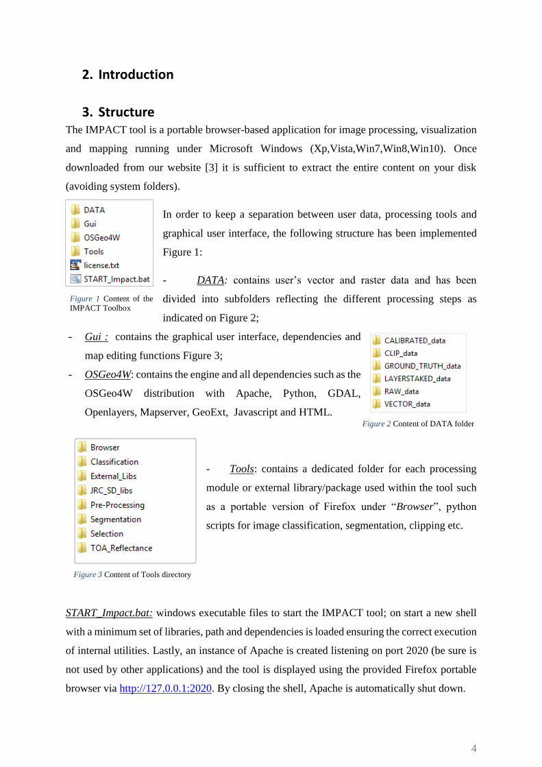
3. Structure The IMPACT tool is a portable browser-based application for image processing, visualization

and mapping running under Microsoft Windows (Xp,Vista,Win7,Win8,Win10). Once

downloaded from our website [3] it is sufficient to extract the entire content on your disk

(avoiding system folders).

In order to keep a separation between user data, processing tools and

graphical user interface, the following structure has been implemented

Figure 1:

- DATA: contains user’s vector and raster data and has been

divided into subfolders reflecting the different processing steps as

indicated on Figure 2;

- Gui : contains the graphical user interface, dependencies and

map editing functions Figure 3;

- OSGeo4W: contains the engine and all dependencies such as the

OSGeo4W distribution with Apache, Python, GDAL,

Openlayers, Mapserver, GeoExt, Javascript and HTML.

- Tools: contains a dedicated folder for each processing

module or external library/package used within the tool such

as a portable version of Firefox under “Browser”, python

scripts for image classification, segmentation, clipping etc.

START_Impact.bat: windows executable files to start the IMPACT tool; on start a new shell

with a minimum set of libraries, path and dependencies is loaded ensuring the correct execution

of internal utilities. Lastly, an instance of Apache is created listening on port 2020 (be sure is

not used by other applications) and the tool is displayed using the provided Firefox portable

browser via http://127.0.0.1:2020. By closing the shell, Apache is automatically shut down.

Figure 1 Content of the

IMPACT Toolbox

Figure 2 Content of DATA folder

Figure 3 Content of Tools directory

5

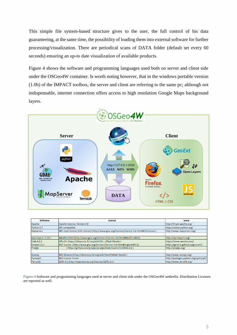
This simple file system-based structure gives to the user, the full control of his data

guaranteeing, at the same time, the possibility of loading them into external software for further

processing/visualization. There are periodical scans of DATA folder (default set every 60

seconds) ensuring an up-to date visualization of available products.

Figure 4 shows the software and programming languages used both on server and client side

under the OSGeo4W container. Is worth noting however, that in the windows portable version

(1.0b) of the IMPACT toolbox, the server and client are referring to the same pc; although not

indispensable, internet connection offers access to high resolution Google Maps background

layers.

Server Client

Portal

Figure 4 Software and programming languages used at server and client side under the OSGeo4W umbrella. Distribution Licenses

are reported as well.

http://127.0.0.1:2020

AJAX WFS WMS

DATA

6

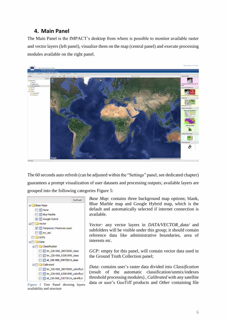
4. Main Panel The Main Panel is the IMPACT’s desktop from where is possible to monitor available raster

and vector layers (left panel), visualize them on the map (central panel) and execute processing

modules available on the right panel.

The 60 seconds auto refresh (can be adjusted within the “Settings” panel, see dedicated chapter)

guarantees a prompt visualization of user datasets and processing outputs; available layers are

grouped into the following categories Figure 5:

Base Map: contains three background map options; blank,

Blue Marble map and Google Hybrid map, which is the

default and automatically selected if internet connection is

available.

Vector: any vector layers in DATA/VECTOR_data/ and

subfolders will be visible under this group; it should contain

reference data like administrative boundaries, area of

interests etc.

GCP: empty for this panel, will contain vector data used in

the Ground Truth Collection panel;

Data: contains user’s raster data divided into Classification

(result of the automatic classification/unmix/indexes

threshold processing modules) , Calibrated with any satellite

data or user’s GeoTiff products and Other containing file Figure 5 Tree Panel showing layers

availability and structure

7

data without default Impact’s suffixes. These data are found in the directory structure under

/DATA/CALIBRATED_data/.

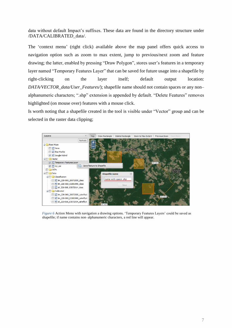
The ‘context menu’ (right click) available above the map panel offers quick access to

navigation option such as zoom to max extent, jump to previous/next zoom and feature

drawing; the latter, enabled by pressing “Draw Polygon”, stores user’s features in a temporary

layer named “Temporary Features Layer” that can be saved for future usage into a shapefile by

right-clicking on the layer itself; default output location:

DATA/VECTOR_data/User_Features/); shapefile name should not contain spaces or any non–

alphanumeric characters; “.shp” extension is appended by default. “Delete Features” removes

highlighted (on mouse over) features with a mouse click.

Is worth noting that a shapefile created in the tool is visible under “Vector” group and can be

selected in the raster data clipping;

Figure 6 Action Menu with navigation a drawing options. ‘Temporary Features Layers’ could be saved as

shapefile; if name contains non–alphanumeric characters, a red line will appear.

8

5. Processing Modules

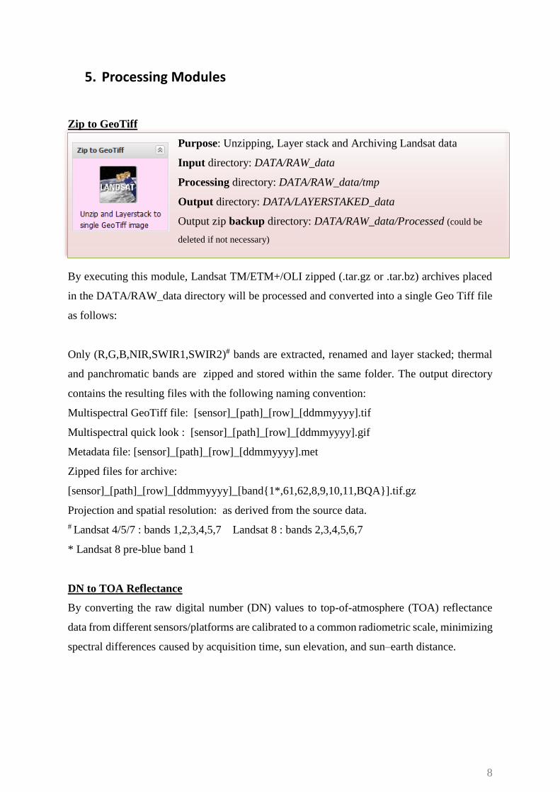
Zip to GeoTiff

Purpose: Unzipping, Layer stack and Archiving Landsat data

Input directory: DATA/RAW_data

Processing directory: DATA/RAW_data/tmp

Output directory: DATA/LAYERSTAKED_data

Output zip backup directory: DATA/RAW_data/Processed (could be

deleted if not necessary)

By executing this module, Landsat TM/ETM+/OLI zipped (.tar.gz or .tar.bz) archives placed

in the DATA/RAW_data directory will be processed and converted into a single Geo Tiff file

as follows:

Only (R,G,B,NIR,SWIR1,SWIR2)# bands are extracted, renamed and layer stacked; thermal

and panchromatic bands are zipped and stored within the same folder. The output directory

contains the resulting files with the following naming convention:

Multispectral GeoTiff file: [sensor]_[path]_[row]_[ddmmyyyy].tif

Multispectral quick look : [sensor]_[path]_[row]_[ddmmyyyy].gif

Metadata file: [sensor]_[path]_[row]_[ddmmyyyy].met

Zipped files for archive:

[sensor]_[path]_[row]_[ddmmyyyy]_[band{1*,61,62,8,9,10,11,BQA}].tif.gz

Projection and spatial resolution: as derived from the source data.

# Landsat 4/5/7 : bands 1,2,3,4,5,7 Landsat 8 : bands 2,3,4,5,6,7

* Landsat 8 pre-blue band 1

DN to TOA Reflectance

By converting the raw digital number (DN) values to top-of-atmosphere (TOA) reflectance

data from different sensors/platforms are calibrated to a common radiometric scale, minimizing

spectral differences caused by acquisition time, sun elevation, and sun–earth distance.

9

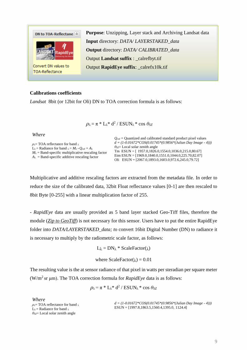
Purpose: Unzipping, Layer stack and Archiving Landsat data

Input directory: DATA/ LAYERSTAKED_data

Output directory: DATA/ CALIBRATED_data

Output Landsat suffix : _calrefbyt.tif

Output RapidEye suffix: _calrefx10k.tif

Calibrations coefficients

Landsat 8bit (or 12bit for Oli) DN to TOA correction formula is as follows:

ρλ = π * Lλ* d2 / ESUNλ * cos θSZ

Multiplicative and additive rescaling factors are extracted from the metadata file. In order to

reduce the size of the calibrated data, 32bit Float reflectance values [0-1] are then rescaled to

8bit Byte [0-255] with a linear multiplication factor of 255.

- RapidEye data are usually provided as 5 band layer stacked Geo-Tiff files, therefore the

module (Zip to GeoTiff) is not necessary for this sensor. Users have to put the entire RapidEye

folder into DATA/LAYERSTAKED_data; to convert 16bit Digital Number (DN) to radiance it

is necessary to multiply by the radiometric scale factor, as follows:

Lλ = DNλ * ScaleFactor(λ)

where ScaleFactor(λ) = 0.01

The resulting value is the at sensor radiance of that pixel in watts per steradian per square meter

(W/m2 sr μm). The TOA correction formula for RapidEye data is as follows:

ρλ = π * Lλ* d2 / ESUNλ * cos θSZ

Where

ρλ= TOA reflectance for band λ

Lλ = Radiance for band λ = Mλ * Qcal + Aλ

Mλ = Band-specific multiplicative rescaling factor

Aλ = Band-specific additive rescaling factor

Qcal = Quantized and calibrated standard product pixel values

d = (1-0.01672*COS(0.01745*(0.9856*(Julian Day Image - 4)))

θSZ= Local solar zenith angle

Tm ESUN = [ 1957.0,1826.0,1554.0,1036.0,215.0,80.67]

Etm ESUN = [1969.0,1840.0,1551.0,1044.0,225.70,82.07]

Oli ESUN = [2067.0,1893.0,1603.0,972.6,245.0,79.72]

Where ρλ= TOA reflectance for band λ

Lλ = Radiance for band λ

θSZ= Local solar zenith angle

d = (1-0.01672*COS(0.01745*(0.9856*(Julian Day Image - 4)))

ESUN = [1997.8,1863.5,1560.4,1395.0, 1124.4]

10

32bit Float reflectance values [0-1] are then rescaled to 16bit Unsigned Integer [0-10000] with

a linear multiplication factor of 10000. Formulas and parameter are derived from [4].

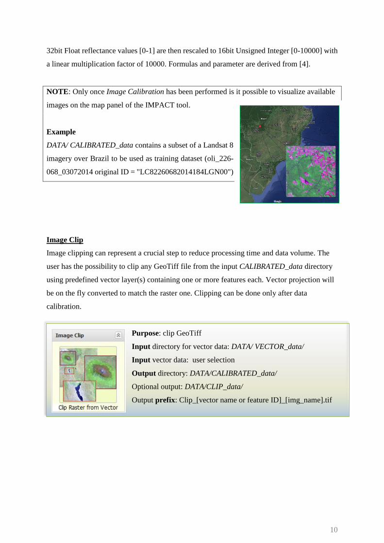
NOTE: Only once Image Calibration has been performed is it possible to visualize available

images on the map panel of the IMPACT tool.

Example

DATA/ CALIBRATED_data contains a subset of a Landsat 8

imagery over Brazil to be used as training dataset (oli_226-

068_03072014 original ID = "LC82260682014184LGN00")

Image Clip

Image clipping can represent a crucial step to reduce processing time and data volume. The

user has the possibility to clip any GeoTiff file from the input CALIBRATED_data directory

using predefined vector layer(s) containing one or more features each. Vector projection will

be on the fly converted to match the raster one. Clipping can be done only after data

calibration.

Purpose: clip GeoTiff

Input directory for vector data: DATA/ VECTOR_data/

Input vector data: user selection

Output directory: DATA/CALIBRATED_data/

Optional output: DATA/CLIP_data/

Output prefix: Clip_[vector name or feature ID]_[img_name].tif

11

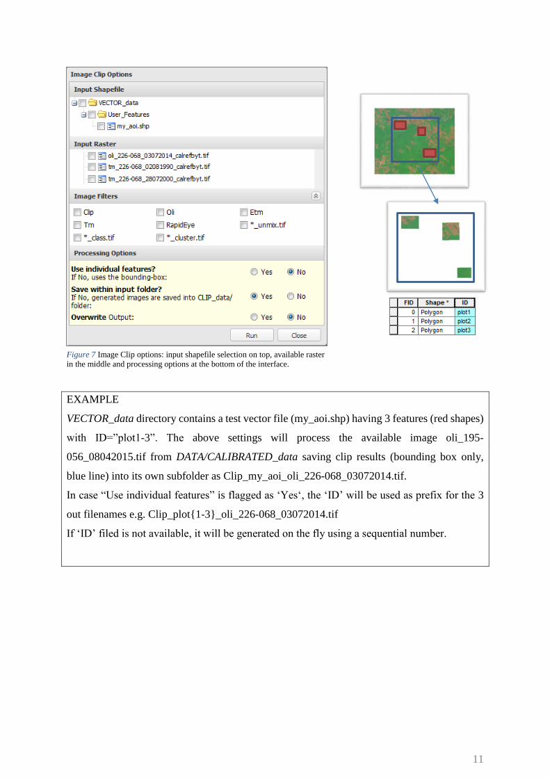
EXAMPLE

VECTOR_data directory contains a test vector file (my_aoi.shp) having 3 features (red shapes)

with ID=”plot1-3”. The above settings will process the available image oli_195-

056_08042015.tif from DATA/CALIBRATED_data saving clip results (bounding box only,

blue line) into its own subfolder as Clip_my_aoi_oli_226-068_03072014.tif.

In case “Use individual features” is flagged as ‘Yes‘, the ‘ID’ will be used as prefix for the 3

out filenames e.g. Clip_plot{1-3}_oli_226-068_03072014.tif

If ‘ID’ filed is not available, it will be generated on the fly using a sequential number.

Figure 7 Image Clip options: input shapefile selection on top, available raster

in the middle and processing options at the bottom of the interface.

12

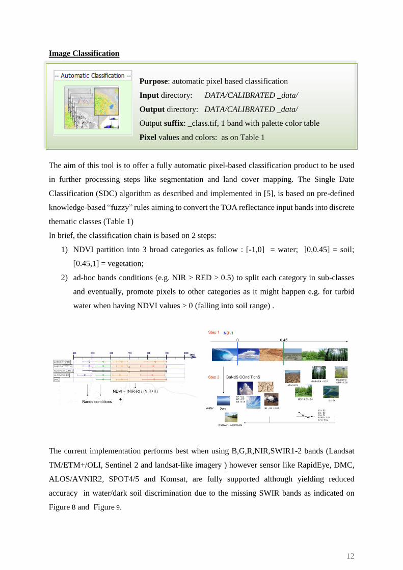
Image Classification

Purpose: automatic pixel based classification

Input directory: DATA/CALIBRATED _data/

Output directory: DATA/CALIBRATED _data/

Output suffix: _class.tif, 1 band with palette color table

Pixel values and colors: as on Table 1

The aim of this tool is to offer a fully automatic pixel-based classification product to be used

in further processing steps like segmentation and land cover mapping. The Single Date

Classification (SDC) algorithm as described and implemented in [5], is based on pre-defined

knowledge-based “fuzzy” rules aiming to convert the TOA reflectance input bands into discrete

thematic classes (Table 1)

In brief, the classification chain is based on 2 steps:

1) NDVI partition into 3 broad categories as follow : [-1,0] = water; ]0,0.45] = soil;

[0.45,1] = vegetation;

2) ad-hoc bands conditions (e.g. NIR > RED > 0.5) to split each category in sub-classes

and eventually, promote pixels to other categories as it might happen e.g. for turbid

water when having NDVI values > 0 (falling into soil range) .

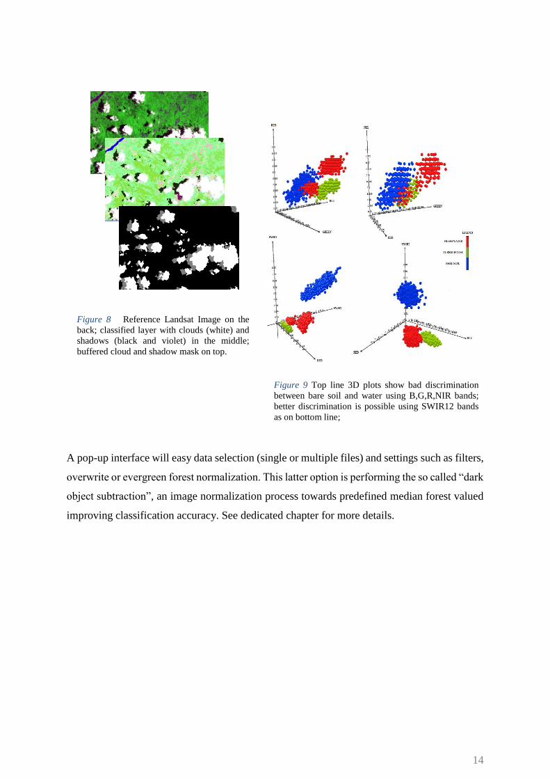
The current implementation performs best when using B,G,R,NIR,SWIR1-2 bands (Landsat

TM/ETM+/OLI, Sentinel 2 and landsat-like imagery ) however sensor like RapidEye, DMC,

ALOS/AVNIR2, SPOT4/5 and Komsat, are fully supported although yielding reduced

accuracy in water/dark soil discrimination due to the missing SWIR bands as indicated on

Figure 8 and Figure 9.

13

Similar SDC algorithm robustness and scalability among the aforementioned sensor have been

confirmed by [6] and [7]; however, SDC’s accuracy is not easily quantifiable since the

algorithm delivers broad thematic categories derived from spectral properties observed during

a precise time in the vegetation cycle; is therefore possible to classify leafs-off deciduous forest

as grass or soil. [5] better explains how to combine and analyze SDCs time series in order to

produce more accurate land cover maps.

Is worth noting the SDC is capable of retrieving sun azimuth from the correspondent metadata

in order to apply post classification 3D models and morphological filters (opening and closing)

for better clouds/shadow masking and “salt and pepper” reduction. As on Table 1, cloudy pixels

(ID 1 and 2) and potential shadow pixels (ID = 10,35,40,41,42 ) are initially treated using the

morphological ‘closing’ filter of 500mt; afterward, cloudy pixels are projected in the sun

azimuth and possible overlaps are automatically recoded as Shadow/Low Illumination

(ID=42).

Please note that on off-nadir acquisition sensor like RapidEye, the relative position of clouds

and their shadows don’t match the provided sun azimuth angle. The apparent cloud shift

distance, in relation to its true position, depends on the off-nadir angle and on the cloud height.

Whereas the satellite off-nadir angle is well known, the height of imaged clouds is unknown

[8]. For this later reason the clouds and shadow masking as provided by SDC might not be

optimal for RapidEye imagery. Ideally the user coul replace the ‘real’ sun azimuth with the

apparent one within the .xml metadata.

14

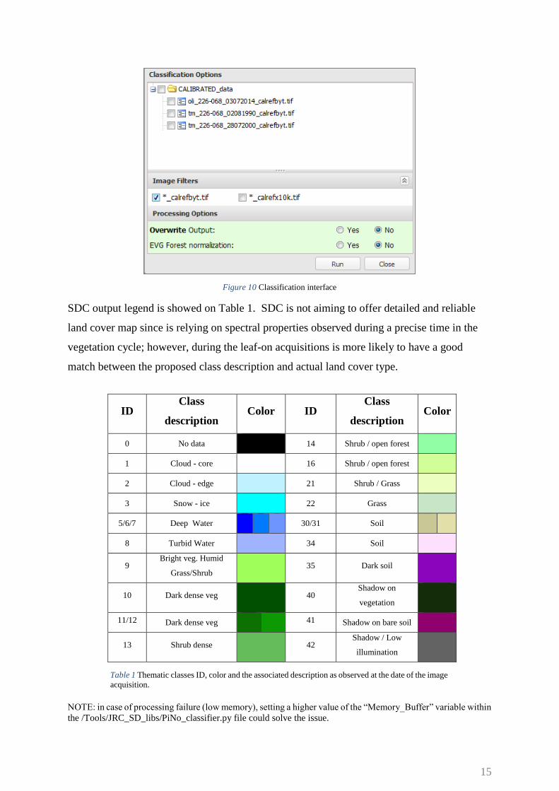
A pop-up interface will easy data selection (single or multiple files) and settings such as filters,

overwrite or evergreen forest normalization. This latter option is performing the so called “dark

object subtraction”, an image normalization process towards predefined median forest valued

improving classification accuracy. See dedicated chapter for more details.

Figure 9 Top line 3D plots show bad discrimination

between bare soil and water using B,G,R,NIR bands;

better discrimination is possible using SWIR12 bands

as on bottom line;

Figure 8 Reference Landsat Image on the

back; classified layer with clouds (white) and

shadows (black and violet) in the middle;

buffered cloud and shadow mask on top.

15

Figure 10 Classification interface

SDC output legend is showed on Table 1. SDC is not aiming to offer detailed and reliable

land cover map since is relying on spectral properties observed during a precise time in the

vegetation cycle; however, during the leaf-on acquisitions is more likely to have a good

match between the proposed class description and actual land cover type.

NOTE: in case of processing failure (low memory), setting a higher value of the “Memory_Buffer” variable within

the /Tools/JRC_SD_libs/PiNo_classifier.py file could solve the issue.

ID Class

description Color ID

Class

description Color

0 No data 14 Shrub / open forest

1 Cloud - core 16 Shrub / open forest

2 Cloud - edge 21 Shrub / Grass

3 Snow - ice 22 Grass

5/6/7 Deep Water 30/31 Soil

8 Turbid Water 34 Soil

9 Bright veg. Humid

Grass/Shrub 35 Dark soil

10 Dark dense veg 40 Shadow on

vegetation

11/12 Dark dense veg 41 Shadow on bare soil

13 Shrub dense 42 Shadow / Low

illumination

Table 1 Thematic classes ID, color and the associated description as observed at the date of the image

acquisition.

16

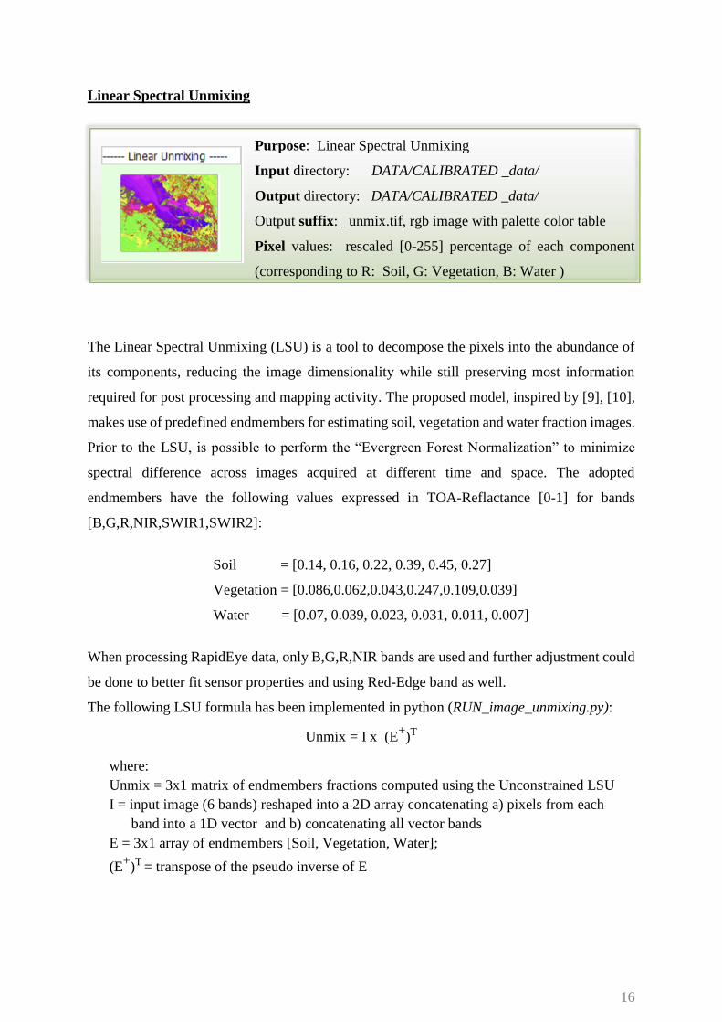
Linear Spectral Unmixing

Purpose: Linear Spectral Unmixing

Input directory: DATA/CALIBRATED _data/

Output directory: DATA/CALIBRATED _data/

Output suffix: _unmix.tif, rgb image with palette color table

Pixel values: rescaled [0-255] percentage of each component

(corresponding to R: Soil, G: Vegetation, B: Water )

The Linear Spectral Unmixing (LSU) is a tool to decompose the pixels into the abundance of

its components, reducing the image dimensionality while still preserving most information

required for post processing and mapping activity. The proposed model, inspired by [9], [10],

makes use of predefined endmembers for estimating soil, vegetation and water fraction images.

Prior to the LSU, is possible to perform the “Evergreen Forest Normalization” to minimize

spectral difference across images acquired at different time and space. The adopted

endmembers have the following values expressed in TOA-Reflactance [0-1] for bands

[B,G,R,NIR,SWIR1,SWIR2]:

Soil = [0.14, 0.16, 0.22, 0.39, 0.45, 0.27]

Vegetation = [0.086,0.062,0.043,0.247,0.109,0.039]

Water = [0.07, 0.039, 0.023, 0.031, 0.011, 0.007]

When processing RapidEye data, only B,G,R,NIR bands are used and further adjustment could

be done to better fit sensor properties and using Red-Edge band as well.

The following LSU formula has been implemented in python (RUN_image_unmixing.py):

Unmix = I x (E+)T

where:

Unmix = 3x1 matrix of endmembers fractions computed using the Unconstrained LSU

I = input image (6 bands) reshaped into a 2D array concatenating a) pixels from each

band into a 1D vector and b) concatenating all vector bands

E = 3x1 array of endmembers [Soil, Vegetation, Water];

(E+)T = transpose of the pseudo inverse of E

17

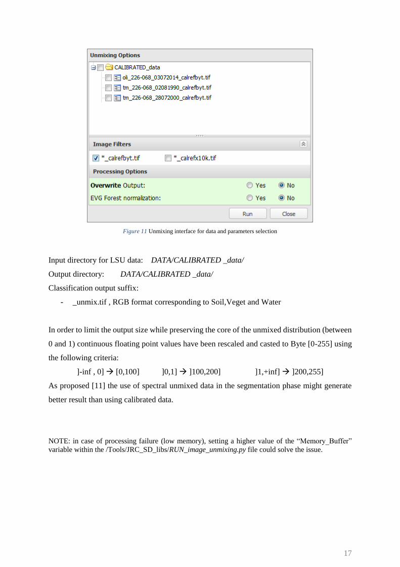
Figure 11 Unmixing interface for data and parameters selection

Input directory for LSU data: DATA/CALIBRATED _data/

Output directory: DATA/CALIBRATED _data/

Classification output suffix:

- _unmix.tif , RGB format corresponding to Soil,Veget and Water

In order to limit the output size while preserving the core of the unmixed distribution (between

0 and 1) continuous floating point values have been rescaled and casted to Byte [0-255] using

the following criteria:

]-inf , 0] [0,100] ]0,1] ]100,200] ]1,+inf] ]200,255]

As proposed [11] the use of spectral unmixed data in the segmentation phase might generate

better result than using calibrated data.

NOTE: in case of processing failure (low memory), setting a higher value of the “Memory_Buffer”

variable within the /Tools/JRC_SD_libs/RUN_image_unmixing.py file could solve the issue.

18

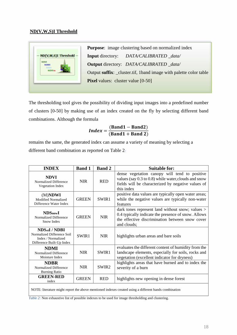
ND(V,W,S)I Threshold

Purpose: image clustering based on normalized index

Input directory: DATA/CALIBRATED _data/

Output directory: DATA/CALIBRATED _data/

Output suffix: _cluster.tif, 1band image with palette color table

Pixel values: cluster value [0-50]

The thresholding tool gives the possibility of dividing input images into a predefined number

of clusters [0-50] by making use of an index created on the fly by selecting different band

combinations. Although the formula

𝑰𝒏𝒅𝒆𝒙 =(𝐁𝐚𝐧𝐝𝟏 − 𝐁𝐚𝐧𝐝𝟐)

(𝐁𝐚𝐧𝐝𝟏 + 𝐁𝐚𝐧𝐝 𝟐)

remains the same, the generated index can assume a variety of meaning by selecting a

different band combination as reported on Table 2:

INDEX Band 1 Band 2 Suitable for:

NDVI Normalized Difference

Vegetation Index NIR RED

dense vegetation canopy will tend to positive

values (say 0.3 to 0.8) while water,clouds and snow

fields will be characterized by negative values of

this index

(M)NDWI Modified Normalized

Difference Water Index GREEN SWIR1

positive data values are typically open water areas;

while the negative values are typically non-water

features

NDSnowI Normalized Difference

Snow Index GREEN NIR

dark tones represent land without snow; values >

0.4 typically indicate the presence of snow. Allows

the effective discrimination between snow cover

and clouds;

NDSoilI / NDBI Normalized Difference Soil

Index / Normalized

Difference Built-Up Index

SWIR1 NIR highlights urban areas and bare soils

NDMI Normalized Difference

Moisture Index NIR SWIR1

evaluates the different content of humidity from the

landscape elements, especially for soils, rocks and

vegetation (excellent indicator for dryness)

NDBR Normalized Difference

Burning Ratio NIR SWIR2

highlights areas that have burned and to index the

severity of a burn

GREEN-RED index

GREEN RED highlights new opening in dense forest

NOTE: literature might report the above mentioned indexes created using a different bands combination

Table 2: Non exhaustive list of possible indexes to be used for image thresholding and clustering.

19

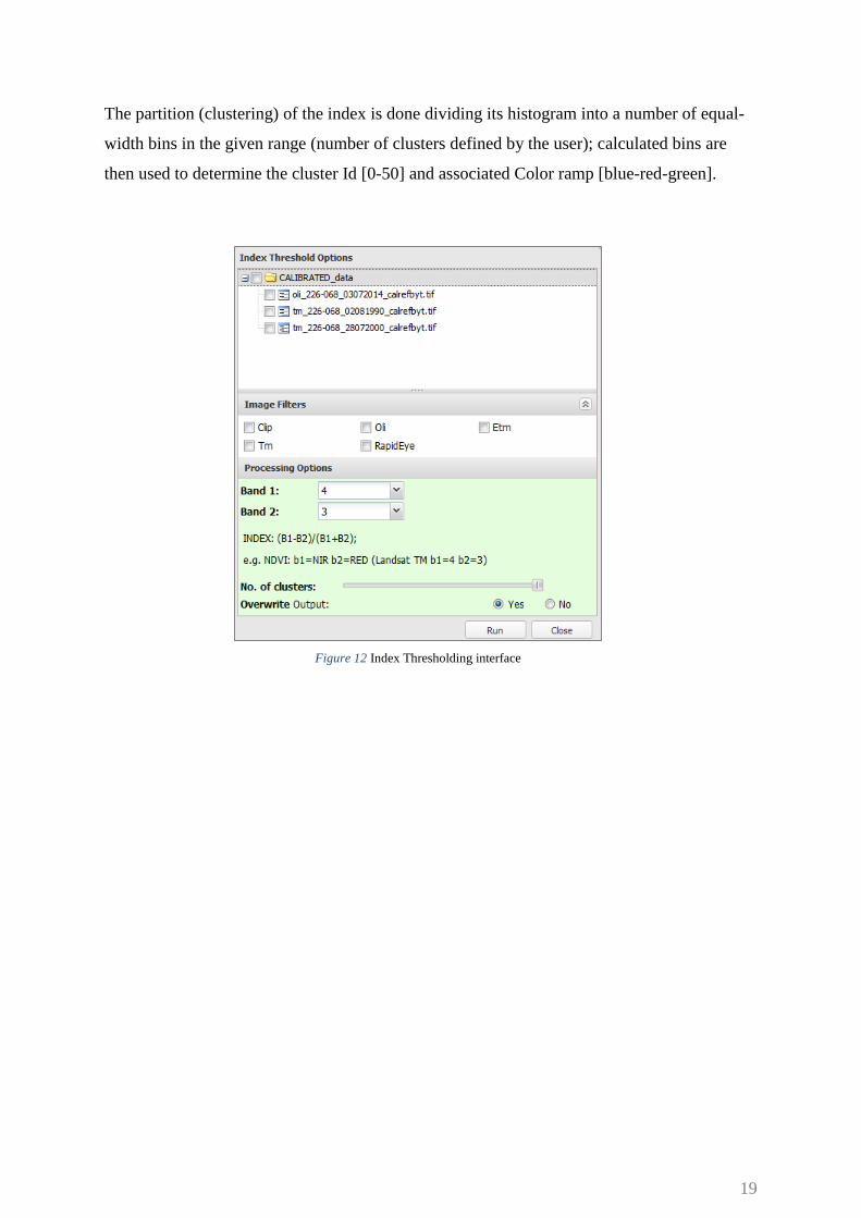
The partition (clustering) of the index is done dividing its histogram into a number of equal-

width bins in the given range (number of clusters defined by the user); calculated bins are

then used to determine the cluster Id [0-50] and associated Color ramp [blue-red-green].

Figure 12 Index Thresholding interface

20

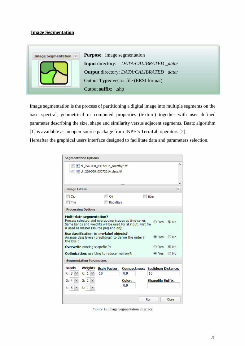
Image Segmentation

Purpose: image segmentation

Input directory: DATA/CALIBRATED _data/

Output directory: DATA/CALIBRATED _data/

Output Type: vector file (ERSI format)

Output suffix: .shp

Image segmentation is the process of partitioning a digital image into multiple segments on the

base spectral, geometrical or computed properties (texture) together with user defined

parameter describing the size, shape and similarity versus adjacent segments. Baatz algorithm

[1] is available as an open-source package from INPE’s TerraLib operators [2].

Hereafter the graphical users interface designed to facilitate data and parameters selection.

Figure 13 Image Segmentation interface

21

Segmentation Options:

- Multi-date segmentation:

o “No”: selected images are treated individually and the correspondent vector file

(ESRI Shapefile format) is saved within the image directory; please ensure that

segmentation parameters are applicable to all selected images, bands selection

above any other.

o “Yes”: selected images are layer stacked (only selected bands) into a single one

using the selected bands and weight. Please ensure the geographical overlap.

First file is use to extract output location and reference projection

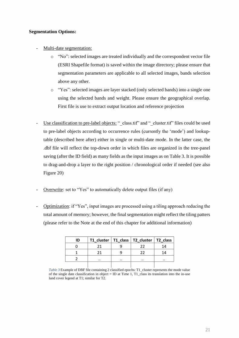
- Use classification to pre-label objects: “_class.tif” and “_cluster.tif” files could be used

to pre-label objects according to occurrence rules (currently the ‘mode’) and lookup-

table (described here after) either in single or multi-date mode. In the latter case, the

.dbf file will reflect the top-down order in which files are organized in the tree-panel

saving (after the ID field) as many fields as the input images as on Table 3. It is possible

to drag-and-drop a layer to the right position / chronological order if needed (see also

Figure 20)

- Overwrite: set to “Yes” to automatically delete output files (if any)

- Optimization: if “Yes”, input images are processed using a tiling approach reducing the

total amount of memory; however, the final segmentation might reflect the tiling patters

(please refer to the Note at the end of this chapter for additional information)

ID T1_cluster T1_class T2_cluster T2_class

0 21 9 22 14

1 21 9 22 14

2 .. .. .. ..

Table 3 Example of DBF file containing 2 classified epochs: T1_cluster represents the mode value

of the single date classification in object = ID at Time 1, T1_class its translation into the in-use

land cover legend at T1; similar for T2.

22

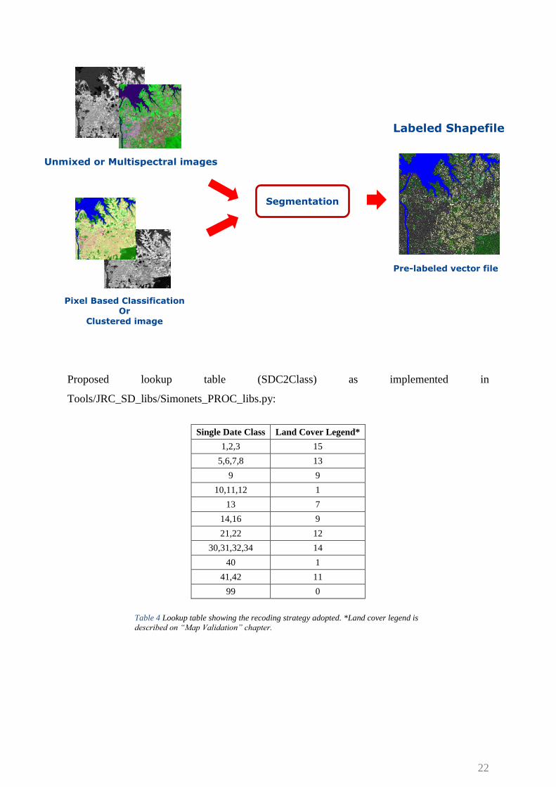
Proposed lookup table (SDC2Class) as implemented in

Tools/JRC_SD_libs/Simonets_PROC_libs.py:

Single Date Class Land Cover Legend*

1,2,3 15

5,6,7,8 13

9 9

10,11,12 1

13 7

14,16 9

21,22 12

30,31,32,34 14

40 1

41,42 11

99 0

Table 4 Lookup table showing the recoding strategy adopted. *Land cover legend is

described on “Map Validation” chapter.

Labeled Shapefile

Pixel Based Classification Or

Clustered image

Segmentation

Unmixed or Multispectral images

Pre-labeled vector file

23

Segmentation Parameters:

- Bands and weights: raster bands and associated weight to be used

- Scale factor: this factor controls the spectral heterogeneity of the image objects and is

therefore correlated with their average size; smaller it is, more objects you will get

- Color: Baatz spectral component [0.0, 1.0]

- Compactness: Baatz morphological component [0.0, 1.0]

- Euclidean distance: used only if the memory “optimization” flag is enabled; represents

the minimum Euclidean Distance (expressed in DN values) to be used while merging

segments crossing two adjacent tiles; higher values will allow aggregation of

heterogeneous objects; lower values will keep the straight edges of the tiles.

- Suffix: user define string (only alphanumeric) to be add to the output filename

NOTE:

- Please ensure that the selected band numbers are available within the raster/s (generic “Baatz

Failure” error message will be raised)

- The multi-date segmentation creates an ancillary file within the directory of the first selected

image (master) containing the name of the processed images and the order of the _class.tif

within the .DBF file

- Objects pre-labeling requires a classified raster _class.tif (e.g. the result of the automatic

classification) from which to extract statistical information from (e.g. the “mode”) together

with a lookup table to convert it into the adopted land cover/use legend. Clustered images

_cluster.tif or user-defined classified raster/maps are accepted but will only be used to fill

the “T(n)_cluster” attribute since the conversion from cluster ID to Land cover/use cannot

be defined a priori. Currently is possible to overcome this limitation by changing the python

class MYmode2D and SDC2Class within the Simonets_PROC_libs.py file

- Big TIFF files are not supported

Segmentation results could be visualized using the Map Validation Panel

Annex1 reports several tests conducted using a different parameters.

24

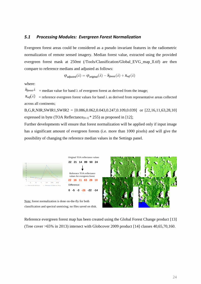
5.1 Processing Modules: Evergreen Forest Normalization

Evergreen forest areas could be considered as a pseudo invariant features in the radiometric

normalization of remote sensed imagery. Median forest value, extracted using the provided

evergreen forest mask at 250mt (/Tools/Classification/Global_EVG_map_ll.tif) are then

compare to reference medians and adjusted as follows:

where:

= median value for band l of evergreen forest as derived from the image;

= reference evergreen forest values for band l as derived from representative areas collected

across all continents;

B,G,R,NIR,SWIR1,SWIR2 = [0.086,0.062,0.043,0.247,0.109,0.039] or [22,16,11,63,28,10]

expressed in byte (TOA Reflectance[0-1] * 255) as proposed in [12];

Further developments will ensure that forest normalization will be applied only if input image

has a significant amount of evergreen forests (i.e. more than 1000 pixels) and will give the

possibility of changing the reference median values in the Settings panel.

Note: forest normalization is done on-the-fly for both

classification and spectral unmixing; no files saved on disk.

Reference evergreen forest map has been created using the Global Forest Change product [13]

(Tree cover >65% in 2013) intersect with Globcover 2009 product [14] classes 40,65,70,160.

22 21 14 89 50 24

22 16 11 63 28 10

Difference:

0 -5 -3 -26 -22 -14

Original TOA reflectance values

Reference TOA reflectance

values for evergreen forest

25

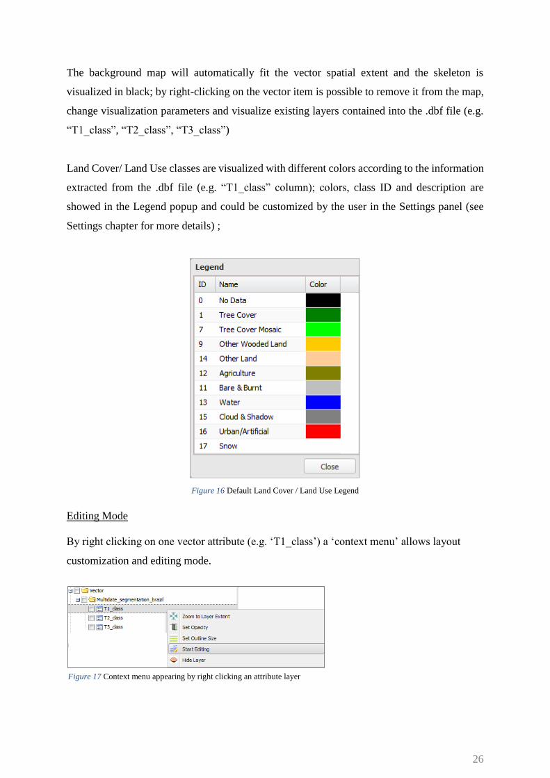
6. Map Validation Panel

Within the Map Validation panel is possible to visualize and edit vector files such as the result

of the segmentation step in order to check and assess the quality of land cover maps. By

clicking on the “Editing Tools” any available vector file (*.shp) within the

/DATA/CALIBRATED_data/ folder could be loaded together with any raster that come along;

files are then visible on the layer tree under the correspondent category; please refer to

“Settings” chapter to better understand input requirements.

Figure 15 Map Validation and Editing Options panels

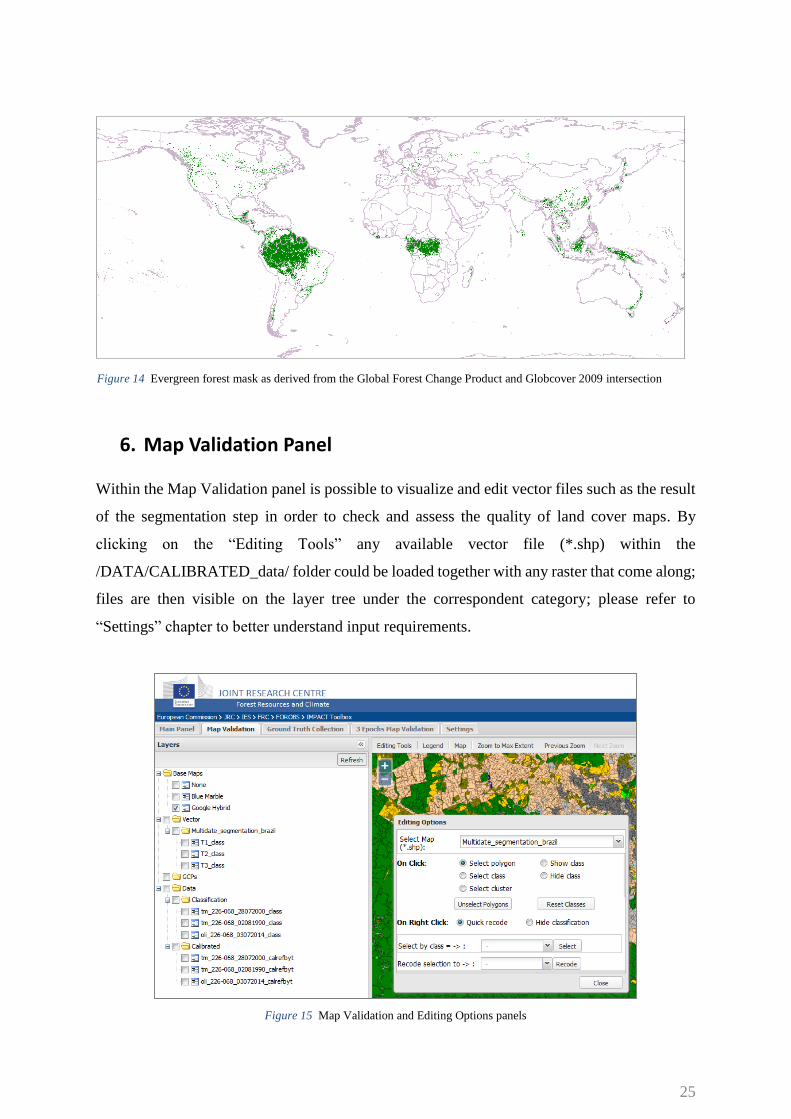
Figure 14 Evergreen forest mask as derived from the Global Forest Change Product and Globcover 2009 intersection

26

The background map will automatically fit the vector spatial extent and the skeleton is

visualized in black; by right-clicking on the vector item is possible to remove it from the map,

change visualization parameters and visualize existing layers contained into the .dbf file (e.g.

“T1_class”, “T2_class”, “T3_class”)

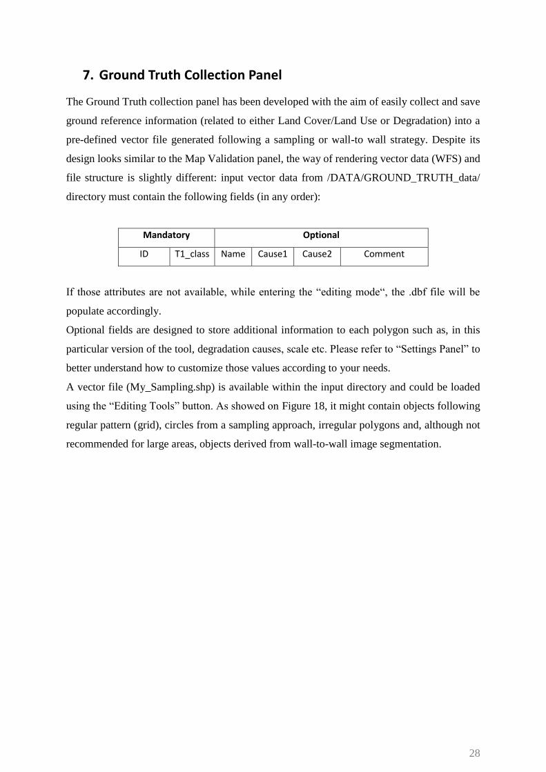
Land Cover/ Land Use classes are visualized with different colors according to the information

extracted from the .dbf file (e.g. “T1_class” column); colors, class ID and description are

showed in the Legend popup and could be customized by the user in the Settings panel (see

Settings chapter for more details) ;

Figure 16 Default Land Cover / Land Use Legend

Editing Mode

By right clicking on one vector attribute (e.g. ‘T1_class’) a ‘context menu’ allows layout

customization and editing mode.

Figure 17 Context menu appearing by right clicking an attribute layer

27

Common navigation/visualization instructions:

- Double left click : zoom in;

- Double right click : zoom out;

- Scrolling wheel : zoom in/out;

- Shift + mouse selection : zoom the desired area of interest;

- Right click will temporary hide any classification layers in order to display either user’s

raster or the background layer;

While in editing mode:

- Navigation to other tabs is disabled;

- Selected layer becomes red and is not possible to edit or delete other layers;

- Is possible to hide/select/recode classes or objects using the “Editing Option” panel;

- Recoding is only applied to objects within the current map extent;

- After single or multi (CTRL+ Left click) polygon selection, a fast recoding popup

legend is also available by pressing the right mouse; is possible to disable this option

by selecting ‘Hide classification’ on right click in the “Editing Option” panel;

- While showing or hiding a class, any class re-assignment (different from the masked

one) will not be visible until the “Unselect Class” button is pressed; although this

behavior might be interpreted like a bug, it has been revealed useful for a) set a

preliminary filter/mask on a class and b) add or remove object from/to other classes

while keeping them masked if not belonging to the filtered class.

NOTE:

- Vector and raster files are visualized as WMS; it might be plausible to face a decreasing of

performances while using vector files with more that 10K features; if so, it might be desirable

to disable the skeleton of vector file under “Vector” branch in the tree-panel avoiding double

visualization in case a classification layer (e.g. T1_class) has been loaded as well

- Raster created within the tool are optimized to be visualized through Mapserver; if coming

from processing done outside the IMPACT we are encouraging running the following

commands and keep the associated .xml file together with the .tif file:

gdal_translate -co COMPRESS=LZW -co TILED=YES -ot Byte -scale -co BIGTIFF=YES IN OUT

gdaladdo OUT 2 4 8 16 32 64 128 256 512 1024 2048 4096

gdalinfo –stats OUT

- When Map Validation panel is active, the automatic scan and refresh of DATA folder is

disabled.

28

7. Ground Truth Collection Panel

The Ground Truth collection panel has been developed with the aim of easily collect and save

ground reference information (related to either Land Cover/Land Use or Degradation) into a

pre-defined vector file generated following a sampling or wall-to wall strategy. Despite its

design looks similar to the Map Validation panel, the way of rendering vector data (WFS) and

file structure is slightly different: input vector data from /DATA/GROUND_TRUTH_data/

directory must contain the following fields (in any order):

Mandatory Optional

ID T1_class Name Cause1 Cause2 Comment

If those attributes are not available, while entering the “editing mode“, the .dbf file will be

populate accordingly.

Optional fields are designed to store additional information to each polygon such as, in this

particular version of the tool, degradation causes, scale etc. Please refer to “Settings Panel” to

better understand how to customize those values according to your needs.

A vector file (My_Sampling.shp) is available within the input directory and could be loaded

using the “Editing Tools” button. As showed on Figure 18, it might contain objects following

regular pattern (grid), circles from a sampling approach, irregular polygons and, although not

recommended for large areas, objects derived from wall-to-wall image segmentation.

29

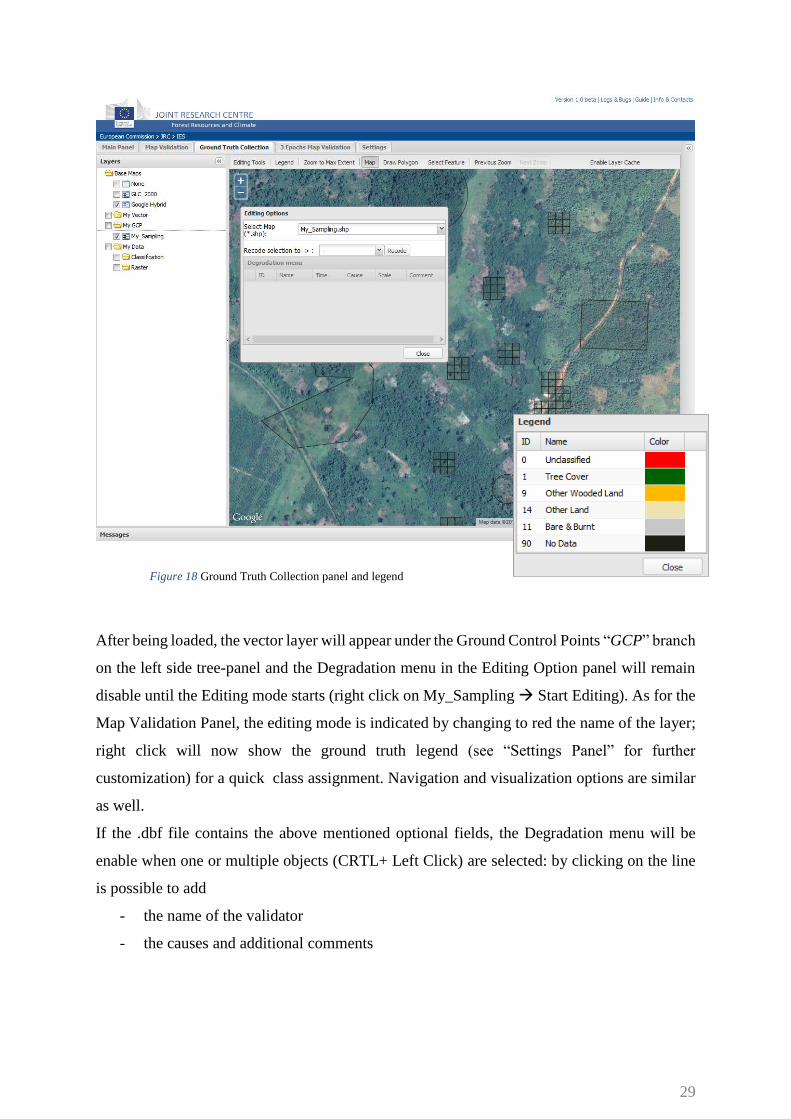
Figure 18 Ground Truth Collection panel and legend

After being loaded, the vector layer will appear under the Ground Control Points “GCP” branch

on the left side tree-panel and the Degradation menu in the Editing Option panel will remain

disable until the Editing mode starts (right click on My_Sampling Start Editing). As for the

Map Validation Panel, the editing mode is indicated by changing to red the name of the layer;

right click will now show the ground truth legend (see “Settings Panel” for further

customization) for a quick class assignment. Navigation and visualization options are similar

as well.

If the .dbf file contains the above mentioned optional fields, the Degradation menu will be

enable when one or multiple objects (CRTL+ Left Click) are selected: by clicking on the line

is possible to add

- the name of the validator

- the causes and additional comments

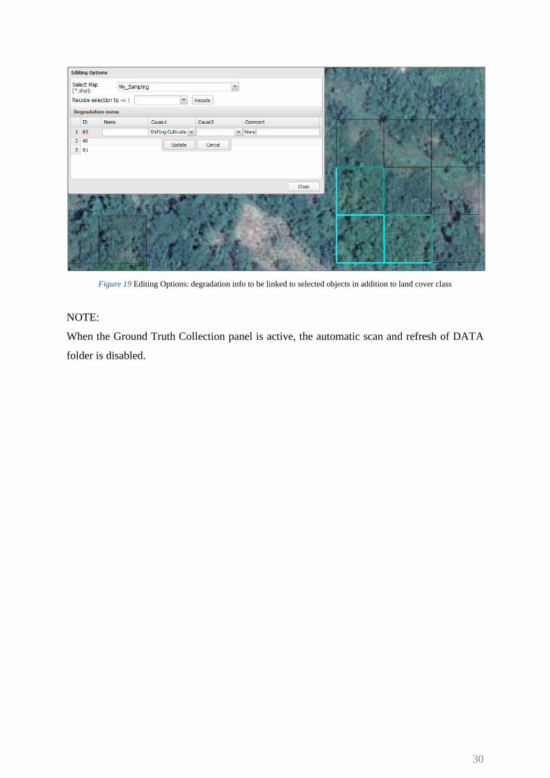
30

Figure 19 Editing Options: degradation info to be linked to selected objects in addition to land cover class

NOTE:

When the Ground Truth Collection panel is active, the automatic scan and refresh of DATA

folder is disabled.

31

8. 3 Epochs Map Validation Panel

This panel has been designed with the aim of integrating and distributing an open source

version of the JRC Land Cover Change Validation Tool [15] originally developed in Interactive

Data Language (IDL) for the Global Forest Resource Assessment (FRA) Remote Sensing

Survey, a FAO land cover/land use mapping initiative under which JRC had cover a key role

in data selection, processing and tools development. While keeping multi date map

visualization (up to tree) and standard editing features, it offers the innovative selection and

recoding strategy based on clusters and classes alternatively. This hybrid editing technique has

been designed and successfully used in [16] for forest cover mapping in Russia and is currently

in use at JRC for land cover/land use change detection and mapping over protected areas in

Africa within the MESA and BIOPAMA project.

For the sake of clarity within the IMPACT tool a cluster represents a set of objects with

common spectral properties (category) as generated by the automatic SDC tool while a class

is the land cover/land use class associate to each object by the interpreter; is worth noting that

one cluster might include objects with different class and vice-versa.

Data preparation

A vector file resulting from a multi date image segmentation (see Image Segmentation chapter

for more details), must have the following structure:

ID T1_cluster T1_class T2_cluster T2_class T3_cluster T3_class

0 2 15 2 15 2 15

- T1,T2 and T3: epochs and associated display from left to right;

- _cluster represents the mode of the single date classification category; could not be

modified

- _class initially filled using the translation schema as proposed on Table 4, it will contain

land cover/land use classes assigned by the interpreter;

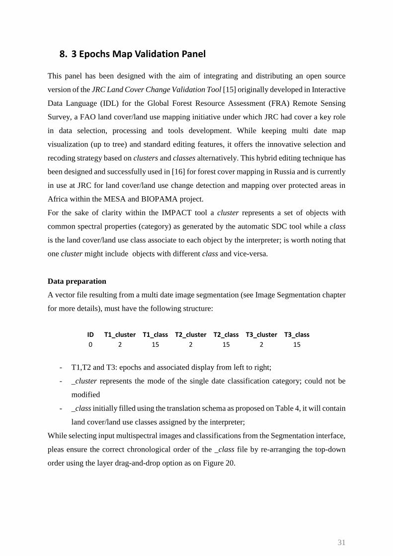
While selecting input multispectral images and classifications from the Segmentation interface,

pleas ensure the correct chronological order of the _class file by re-arranging the top-down

order using the layer drag-and-drop option as on Figure 20.

32

If needed, an ancillary text file containing the list and order of the images used, is available in

the same output directory; for the proposed segmentation test it contains the following lines:

Master Image: W:/DATA/CALIBRATED_data/tm_195-056_18011986_calrefbyt.tif

Other image: W:/DATA/CALIBRATED_data/etm_195-056_02022000_calrefbyt.tif Other image: W:/DATA/CALIBRATED_data/oli_195-056_08042015_calrefbyt.tif

Classification order in DBF :

Classification: W:/DATA/CALIBRATED_data/tm_195-056_18011986_class.tif Classification: W:/DATA/CALIBRATED_data/etm_195-056_02022000_class.tif

Classification: W:/DATA/CALIBRATED_data /oli_195-056_08042015_class.tif

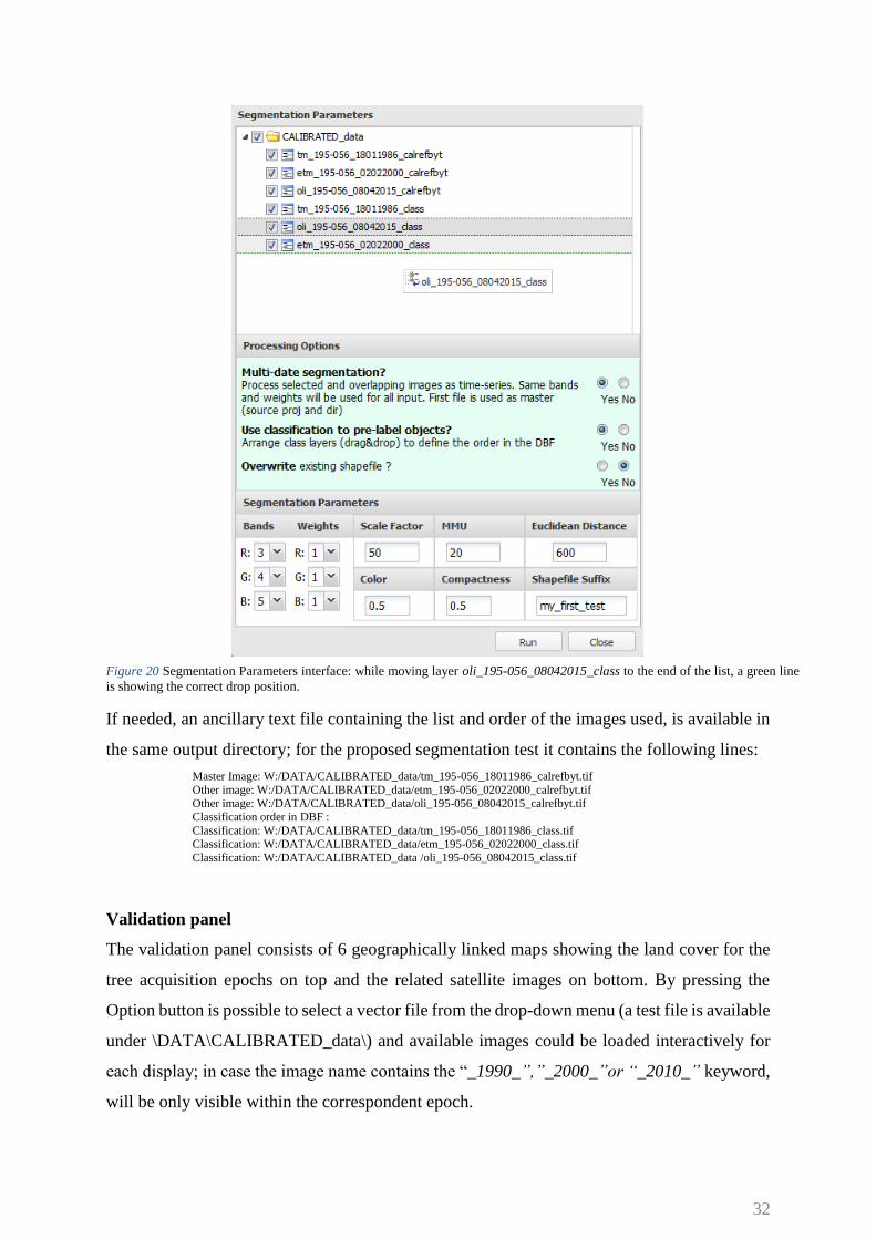
Validation panel

The validation panel consists of 6 geographically linked maps showing the land cover for the

tree acquisition epochs on top and the related satellite images on bottom. By pressing the

Option button is possible to select a vector file from the drop-down menu (a test file is available

under \DATA\CALIBRATED_data\) and available images could be loaded interactively for

each display; in case the image name contains the “_1990_”,”_2000_”or “_2010_” keyword,

will be only visible within the correspondent epoch.

Figure 20 Segmentation Parameters interface: while moving layer oli_195-056_08042015_class to the end of the list, a green line

is showing the correct drop position.

33

Figure 21 3 Epochs Map Validation panel: land cover/land use maps on top and satellite imagery on the bottom for the tree

different acquisition times (left to right); selected clusters are visualized in violet.

By changing the raster visualization option is possible to select the most suitable band

combination and stretch among a predefine selection such as ‘Scale 0-255’, ‘Min-Max’ and

‘1x/2x Standard Deviation’.

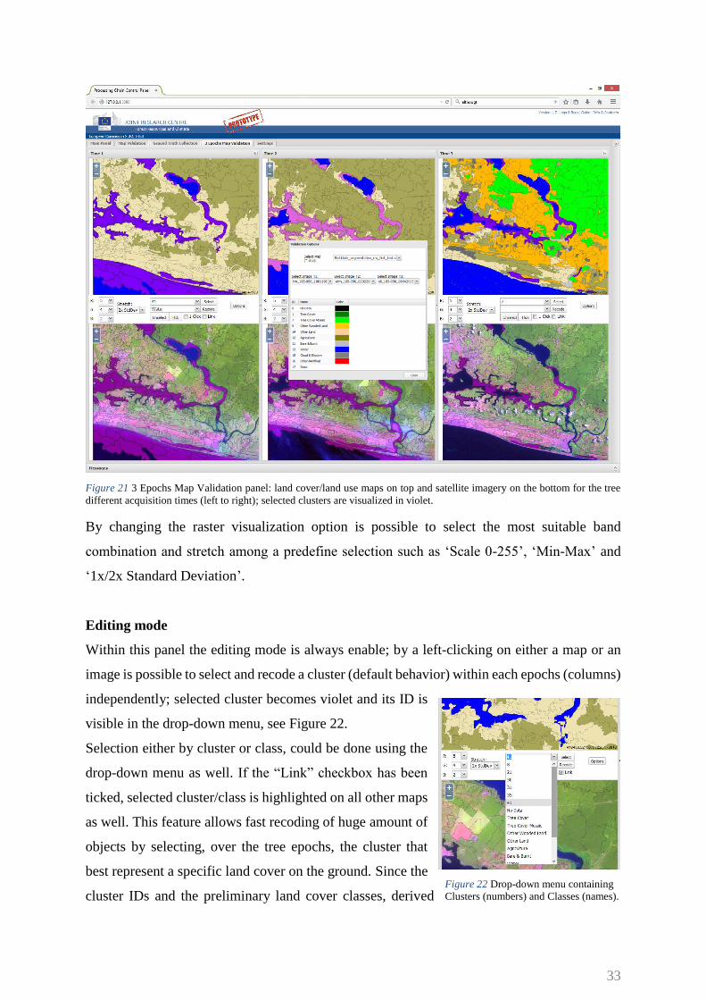
Editing mode

Within this panel the editing mode is always enable; by a left-clicking on either a map or an

image is possible to select and recode a cluster (default behavior) within each epochs (columns)

independently; selected cluster becomes violet and its ID is

visible in the drop-down menu, see Figure 22.

Selection either by cluster or class, could be done using the

drop-down menu as well. If the “Link” checkbox has been

ticked, selected cluster/class is highlighted on all other maps

as well. This feature allows fast recoding of huge amount of

objects by selecting, over the tree epochs, the cluster that

best represent a specific land cover on the ground. Since the

cluster IDs and the preliminary land cover classes, derived Figure 22 Drop-down menu containing

Clusters (numbers) and Classes (names).

34

from the SDC, might not be the same across the tree images due to seasonal differences,

atmospheric conditions or natural/anthropogenic changes we would like to remark that often

the best match between a cluster/class and ground cover might come from a different epoch.

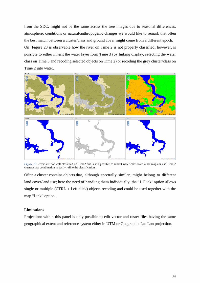
On Figure 23 is observable how the river on Time 2 is not properly classified; however, is

possible to either inherit the water layer form Time 3 (by linking display, selecting the water

class on Time 3 and recoding selected objects on Time 2) or recoding the grey cluster/class on

Time 2 into water.

Figure 23 Rivers are not well classified on Time2 but is still possible to inherit water class from other maps or use Time 2

cluster/class combination to easily refine the classification.

Often a cluster contains objects that, although spectrally similar, might belong to different

land cover/land use; here the need of handling them individually: the “1 Click’ option allows

single or multiple (CTRL + Left click) objects recoding and could be used together with the

map “Link” option.

Limitations

Projection: within this panel is only possible to edit vector and raster files having the same

geographical extent and reference system either in UTM or Geographic Lat-Lon projection.

35

9. Settings Panel

The Settings Panel offers an easy way to customize the behavior and layout of the tool. Settings

are grouped into different tabs as follow:

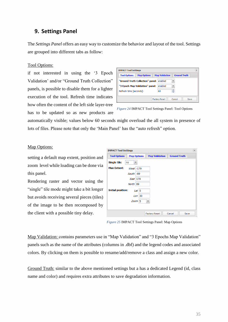
Tool Options:

if not interested in using the ‘3 Epoch

Validation’ and/or “Ground Truth Collection”

panels, is possible to disable them for a lighter

execution of the tool. Refresh time indicates

how often the content of the left side layer-tree

has to be updated so as new products are

automatically visible; values below 60 seconds might overload the all system in presence of

lots of files. Please note that only the ‘Main Panel’ has the “auto refresh” option.

Map Options:

setting a default map extent, position and

zoom level while loading can be done via

this panel.

Rendering raster and vector using the

“single” tile mode might take a bit longer

but avoids receiving several pieces (tiles)

of the image to be then recomposed by

the client with a possible tiny delay.

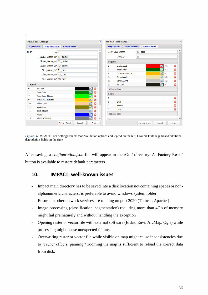
Map Validation: contains parameters use in “Map Validation” and “3 Epochs Map Validation”

panels such as the name of the attributes (columns in .dbf) and the legend codes and associated

colors. By clicking on them is possible to rename/add/remove a class and assign a new color.

Ground Truth: similar to the above mentioned settings but a has a dedicated Legend (id, class

name and color) and requires extra attributes to save degradation information.

Figure 24 IMPACT Tool Settings Panel: Tool Options

Figure 25 IMPACT Tool Settings Panel: Map Options

36

.

After saving, a configuration.json file will appear in the /Gui/ directory. A ‘Factory Reset’

button is available to restore default parameters.

10. IMPACT: well-known issues

- Impact main directory has to be saved into a disk location not containing spaces or non-

alphanumeric characters; is preferable to avoid windows system folder

- Ensure no other network services are running on port 2020 (Tomcat, Apache )

- Image processing (classification, segmentation) requiring more than 4Gb of memory

might fail prematurely and without handling the exception

- Opening raster or vector file with external software (Erdas, Envi, ArcMap, Qgis) while

processing might cause unexpected failure.

- Overwriting raster or vector file while visible on map might cause inconsistencies due

to ‘cache‘ effects; panning / zooming the map is sufficient to reload the correct data

from disk.

Figure 26 IMPACT Tool Settings Panel: Map Validation options and legend on the left; Ground Truth legend and additional

degradation fields on the right

37

11. IMPACT: future developments …

General:

Unix and Windows portability;

Processing:

- Customization of the pre-labeling phase during image segmentation to better match

single date classification schema with the user define land cover classes;

- Image normalization and linear spectral unmixing based on user AOI selection with the

possibility of saving it as vector file;

- Change detection base on two or more images

- RapidEye classification improvements

- Include processing modules for Spot and Sentinel 2 data as well.

Map Validation:

- Undo map editing ;

- Possibility to copy classification (entirely or partially) from one layer (epoch) to

another;

- Changes extraction between different land cover maps

3 Epochs Map Validation:

- Undo map editing ;

- Overpass the limitation of using 3 dates with a flexible and highly customizable

interface;

- Adding the possibility of subtracting clusters from different maps to improve the

selection process;

Ground Truth Collection:

- Confusion matrix and accuracy estimation by comparing ground truths with land

cover maps.

- Automatic generation of sample point / fishnet

38

12. Version This document version 1.0 dated 10/2015 is referring to the IMPACT toolbox 1.0beta.

Please check the last version on http://forobs.jrc.ec.europa.eu/products/software

13. License The IMPACT toolbox is distribute under the GNU General Public License (GPLv3). Please

refer to http://www.gnu.org/licenses/gpl-3.0.en.html to access the official versions of the

license together with a preamble explaining the purpose of this Free/Open Source Software

License.

The toolbox includes a number of subcomponents with separate copyright notices and license

terms. Your use of the source code for these subcomponents is subject to the terms and

conditions stated in the correspondent License.txt file available at:

Apace: \OSGeo4W\apache\ LICENSE.txt

OpenLayers: \Gui\libs\OpenLayers-2.13.1\license.txt

GeoExt: \Gui\libs\geoext2-2.0.1\license.txt

ExtJs: \Gui\libs\ext-4.2.1.883\license.txt

Python: \OSGeo4W\apps\Python27\ LICENSE.txt

PyMorph: \OSGeo4W\apps\Python27\Lib\site-packages\pymorph\README.rst

Gdal/Ogr: \OSGeo4W\share\gdal\LICENSE.TXT

Szip library : \OSGeo4W\etc\licenses\szip-2.1-1.txt

Firefox Portable : \Tools\Browser\FirefoxPortable\Other\Source\License.txt

14. Copyright

Copyright (c) 2015, European Union

All rights reserved.

Redistribution and use in source and binary forms, with or without modification, are permitted

provided that the following conditions are met:

- redistributions of source code must retain the above copyright notice, this list of conditions

and the following disclaimer.

- redistributions in binary form must reproduce the above copyright notice, this list of

conditions and the following disclaimer in the documentation and/or other materials

provided with the distribution.

39

The IMPACT Toolbox is provided by the copyright holders and contributors "as is" and any

express or implied warranties, including, but not limited to, the implied warranties of

merchantability and fitness for a particular purpose are disclaimed. In no event shall the

copyright owner or contributors be liable for any direct, indirect, incidental, special, exemplary,

or consequential damages (including, but not limited to, procurement of substitute goods or

services; loss of use, data, or profits; or business interruption) however caused and on any

theory of liability, whether in contract, strict liability, or tort (including negligence or

otherwise) arising in any way out of the use of this software, even if advised of the possibility

of such damage.

Acknowledgments

Authors would like to thank the valuable contributions and feedbacks of Shimabukuro Y. of

the National Institute for Space Research (Brazil), Grecchi R., Carboni S., Langner A.,

Verhegghen A., Beuchle R., Stibig H.J. of the Forest Resources and Climate Unit – JRC and

Lupi A., Szantoi Z., Roca P., Lorent H., Brink A. of the Land Resource Monitoring Unit –JRC.

A special tank to Thales Sehn Korting of the National Institute for Space Research, Brazil for

helping in compiling a customized windows (.exe) version of the TerraLib Baatz Segmenter.

We're also grateful to all our partners who contributed in testing and debugging the beta version

of the tool reporting impressions, suggestions, and ideas for improvement:

- Laboratório de Monitoramento Ambiental, EMBRAPA Florestas, Brazil

- Institutions and related partners involved in RECAREDD, MESA, PACSBIO

- The Water Resources Unit, JRC, IT

40

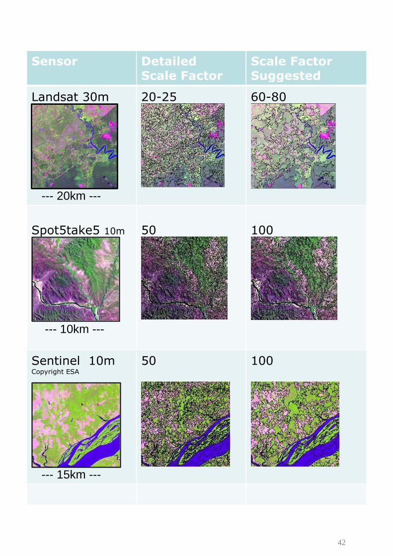
Annex 1: Image segmentation Suggesting a default set of parameters to be used for image segmentation is not often possible;

image size, resolution, data type (byte, integer, float) and nonetheless, the landscape

fragmentation may vary significantly from biome to biome; however, this chapter gives an

overview of the main parameter involved and the different results obtained by using different

acquisition sensors.

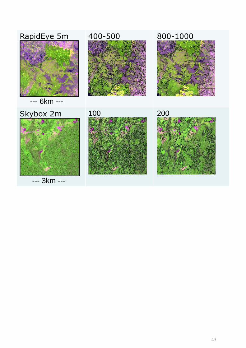
- Scale Factor: “key” parameter, controls size and heterogeneity of the objects

SF 80 SF 10

Landsat image (pan-sharpening 15m 16bit) subset 20x20km

868 Segments Min 0.3ha Max 482ha Mean 46ha 48.637 Segments Min 0.0225ha (pixel size) Max 18ha Mean 0.8ha

- Bands and Weights: selection of bands and relative weight to be used for image

segmentation

Attention: bands selection order doesn’t influence the final results.

18

ha

0.3h

a

482

ha

0.02ha

a

18

ha

41

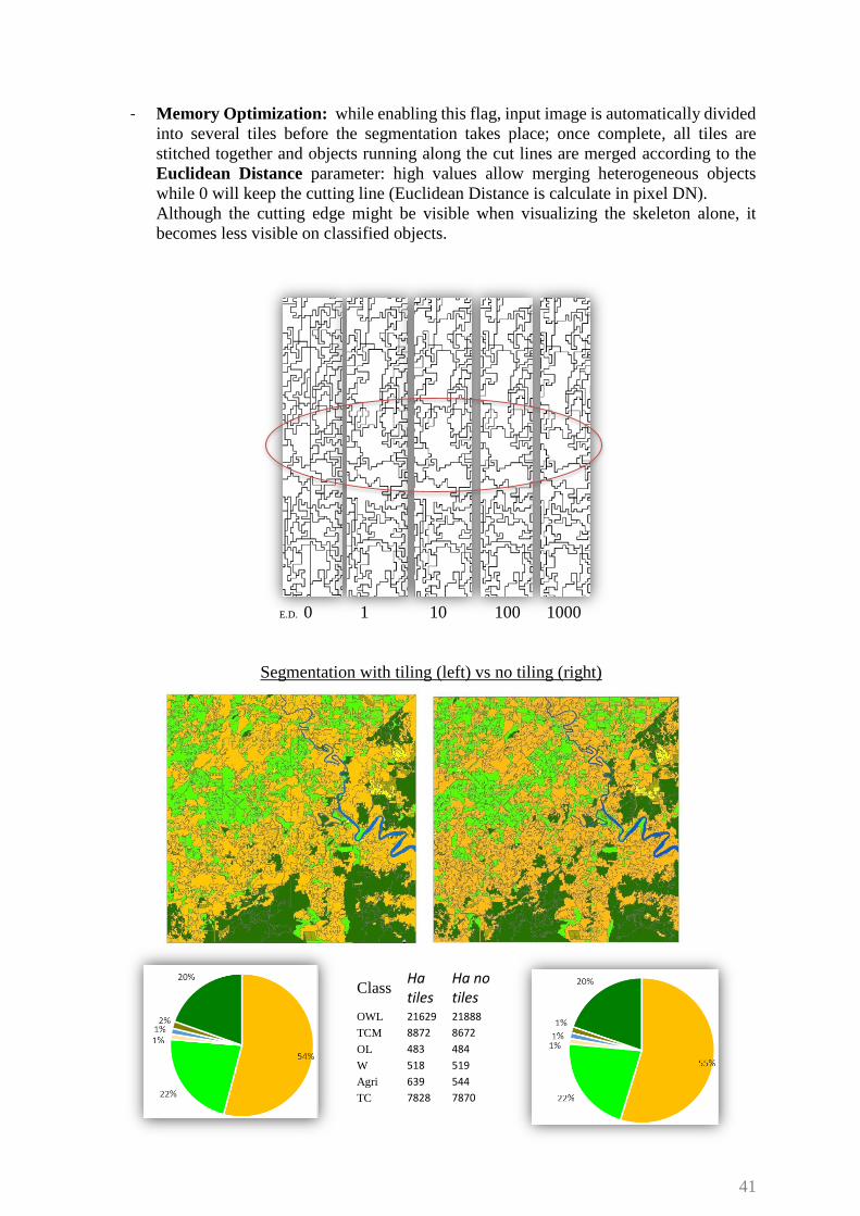
- Memory Optimization: while enabling this flag, input image is automatically divided

into several tiles before the segmentation takes place; once complete, all tiles are

stitched together and objects running along the cut lines are merged according to the

Euclidean Distance parameter: high values allow merging heterogeneous objects

while 0 will keep the cutting line (Euclidean Distance is calculate in pixel DN).

Although the cutting edge might be visible when visualizing the skeleton alone, it

becomes less visible on classified objects.

E.D. 0 1 10 100 1000

Segmentation with tiling (left) vs no tiling (right)

Class Ha tiles

Ha no tiles

OWL 21629 21888

TCM 8872 8672

OL 483 484

W 518 519

Agri 639 544

TC 7828 7870

42

Sensor Detailed Scale Factor

Scale Factor Suggested

Landsat 30m

--- 20km ---

20-25

60-80

Spot5take5 10m

--- 10km ---

50

100

Sentinel 10m Copyright ESA

--- 15km ---

50

100

43

RapidEye 5m

--- 6km ---

400-500

800-1000

Skybox 2m

--- 3km ---

100

200

44

Works Cited

[1] Baatz, M.; Schäpe, A., "Multiresolution segmentation: an optimization approach for high

quality multi-scale image segmentation," in XII Angewandte Geographische

Informationsverarbeitung, Heidelberg, 2000.

[2] Câmara, G., Vinhas, L., Ferreira, K., Queiroz, G., Souza, R., "TerraLib: An open source GIS

library for largescale environmental and socio-economic applications.," Open Source, pp.

247-270, 2008.

[3] JRC, Forest Resources and Climate Unit ,

"http://forobs.jrc.ec.europa.eu/products/software.php," [Online].

[4] RapidEye Satellite Imagery Product Specifications,

"http://www.blackbridge.com/rapideye/upload/RE_Product_Specifications_ENG.pdf,"

[Online].

[5] Simonetti, D.; Simonetti, E.; et al,, "First results from the phenology-based synthesis

classifier using Landsat 8 imagery," IEEE Geoscience and remote sensing letters, 2015.

[6] Szantoi Z., Simonetti D., "Fast and robust topographic correction method for medium

resolution satellite imagery using a stratified approach," IEEE J. Sel. Top. Appl. Earth

Obs. Remote Sens., vol. 6, p. 1921–1933, 2013.

[7] Baraldi, A. et al, "Automatic spectral-rule-based preliminary classification of radiometrically

calibrated SPOT-4/-5/IRS,

AVHRR/MSG,AATSR,IKONOS/QuickBird/OrbView/GeoEye and DMC/SPOT-1/-2

imagery; Part I: System design and implementation," IEEE Trans. Geosci. Remote Sens.,

vol. 48, p. 1299–1325, 2010.

[8] Apparent Cloud Shift in RapidEye Imagery,

"http://blackbridge.com/rapideye/upload/Apparent%20Cloud%20Shift_Final.pdf,"

[Online].

[9] Forrest, G. et al.,, "Remote Sensing of Forest Biophysical Structure Using Mixture

Decomposition and Geometric Reflectance Models," Ecological Applications, vol. 5, no.

4, pp. 993-1013, 1995.

[10] Shimabukuro, Y.E., "Landsat derived shade images of forested areas," in International

Society for photogrammetry and remote sensing, 1988.

[11] Shimabukuro Y.E., et al. , "Using shade fraction image segmentation to evaluate

deforestation in Landsat Thematic Mapper images of the Amazon Region," Int. J.

Remote Sensing, vol. 19, no. 3, pp. 535-541, 1998.

[12] Catherine B., et al., "Pre-processing of a sample of multi-scene and multi-date Landsat

imagery used to monitor forest cover changes over the tropics," ISPRS Journal of

Photogrammetry and Remote Sensing, vol. 66, pp. 555-563, 2011.

[13] Hansen, M. et al., "High-Resolution Global Maps of 21st-Century Forest Cover Change,"

Science, vol. 342, pp. pp. 850-853, 2013.

[14] Arino O., et al., "GlobCover 2009," in ESA Living Planet Symposium, Bergen, Norway,

2010.

[15] Simonetti, D., at al., "User Manual for the JRC Land Cover/Use Change Validation Tool,"

Publications Office of the European Union, Luxembourg, 2011.

[16] S. Bartalev, "Assessment of forest cover in Russia by combining a wall-to-wall coarse-

resolution land-cover map with a sample of 30 m resolution forest maps," International

Journal of Remote Sensing, vol. 35, no. 7, pp. 2671-2692, 2014.

45

Europe Direct is a service to help you find answers to your questions about the European Union

Freephone number (*): 00 800 6 7 8 9 10 11

(*) Certain mobile telephone operators do not allow access to 00 800 numbers or these calls may be billed.

A great deal of additional information on the European Union is available on the Internet.

It can be accessed through the Europa server http://europa.eu.

How to obtain EU publications

Our publications are available from EU Bookshop (http://bookshop.europa.eu),

where you can place an order with the sales agent of your choice.

The Publications Office has a worldwide network of sales agents.

You can obtain their contact details by sending a fax to (352) 29 29-42758.

European Commission

EUR 27358 EN – Joint Research Centre – Institute for Environment and Sustainability

Title: IMPACT: Portable GIS toolbox for image processing and land cover mapping

Authors: Dario Simonetti, Andrea Marelli, Hugh Eva

Luxembourg: Publications Office of the European Union

2015 – 45 pp. – 21.0 x 29.7 cm

EUR – Scientific and Technical Research series – ISSN 1831-9424

ISBN 978-92-79-50115-9

doi:10.2788/143497

46

ISBN 978-92-79-50115-9

x

doi:10.2788/143497

JRC Mission

As the Commission’s in-house science service, the Joint Research Centre’s mission is to provide EU policies with independent, evidence-based scientific and technical support throughout the whole policy cycle.

Working in close cooperation with policy Directorates-General, the JRC addresses key societal challenges while stimulating innovation through developing new methods, tools and standards, and sharing its know-how with the Member States, the scientific community and international partners.

Serving society Stimulating innovation Supporting legislation

LB

-NA

-27358 -E

N-N