June, 1968

STATION BUUETIN 498

DAmy ADJUstMtmS IN tHE NORtHEASt An Analysis 01 Potential Production and

Market Equilibrium

DEPARTMENT OF RESOURCE ECONOMICS NEW HAMPSHIRE AGRICULTURAL EXPERIMENT STATION

UNIVERSITY OF NEW HAMPSHIRE DURHAM, NEW HAMPSHIRE

ANDREW M. NOYAKOV\C AGR\CULTURAL ECO NOMICS

in cooperation with the Farm production EconQJDles Division

Economic Beaeareh Service U. S. Department of Acrieulture

Preface

In dairy farming, as in many other agricultural industries, a major problem is that of adjusting future production to prospective demand. While many adjustment problems may be considered from the view­point of the individual farmer, aggregate production response is the key to this problem. The effects of individual adjustments upon aggre­gate production must be estimated. This aggregation of individual ad· justments to find the production response of an industry has been termed the "micro to macro" approach. It entails developing farm adjustment models and farm situations, solving them for optimal adjustments for a series of prices, and aggregating the resultant output to determine an aggregate supply function.

On the demand side, institutional and transportation costs have tended to preserve the fluid milk markets of the Northeast for local producers. However, there has been substantial net inshipments of ma_n­ufactured milk products from the Lake States area. The future position of dairy farming in the Northeast depends upon changes in both the supply and demand structures for milk.

This study combines an aggregate supply analysis from the micro to macro approach with a set of synthesized demand relationships which reflect the institutional structure of milk marketing in the Northeast. Two dates, 1960 and 1965, are used in the analysis to point out some of the changes which have occurred over this recent time period.

It should be recognized that this is a normative analysis and, as such, is concerned with the potential milk supply if all farmers were to adjust in unison to achieve optimal organization in response to prevail­ing milk prices, factor costs, and technology. The study thus considers the changes in the potential supply of milk as indicative of changes to expect in actual milk supplies. Parts of this analysis are comparable to the Lake States Dairy Adjustment Study.

Since 1960 State Agricultural Experiment Stations in Maine, New Hampshire, Vermont, Massachusetts, Connecticut, New York, New Jersey, Pennsylvania, Maryland, Delaware, and West Virginia and the Farm Production Economics Division, Economic Research Service, U.S. Department of Agriculture, have cooperated in a coordinated study of profitable individual farm and aggregate production adjustments in the Northeast dairy region.

This report is a joint effort of the members of the Northeast Dairy Adjustments Committee. The Committee membership is listed by insti­tution as follows:

1

NORTHEAST DAIRY ADJUSTMENTS STUDY COMMITTEE Institutions and Representatives

University of Connecticut

Cornell University

University of Delaware

University of Maine

University of Maryland

University of Massachusetts

University of New Hampshire

The Pennsylvania State University

Rutgers University University of Vermont

University of West Virginia U.S. Department of Agriculture

Economic Research Service Farm Production Economics Division Washington, D. C .

.. Active at time of publication.

2

M. W.Kotte* G. A. Zepp ~- (USDA) R.Barker D. H. Harrington" (USDA ) B. F. Stanton * G. J. Conneman-' W. M. Crosswhite J. EIterich ¥,-

R. N. Krofta" H. B. Metzger E. S. Micka * (USDA) J. W. Wysong* J. P. Marshall B. D. Crossmon E. I. Fuller'-R. A. Andrews" G. E. Frick" (USDA) W. L.Barr R. T. Dailey (USDA) R. H. McAlexander* K. H. Myers (USDA) E. J. Partenheimer* s. J. Sheehy P. S. DhiIlon~ R. O. Sinclair" R. H. Tremblay¥.-P. E. NesseIroad -;. W. R. Butcher C. W. Crickman* L. M .. Day w. N. Schaller*

Table of Contents

Page Preface 1

Dairy Adjustments in the Northeast 5 An Analysis of Potential Production and Market Equilibrium .5 Objectives . . . ... ....... 6

Description of the Northeast Dairy Region . Characteristics of the Northeast Dairy Region Characteristics of Commercial Dairy Farms Market Structure and Pricing Consumption and Utilization

Methodology for Establishing Supply Functions Selection of Areas Within the Northeast Farm Sample and Sampling Procedure New England New York, New Jersey, Northern Pennsylvania P ennsylvania, Maryland, Delaware, and West Virginia Farm Survey Data Other Data

Metbod of Developing Representative Farms Grouping of Farms Development of Restrictions and Machinery Complements

The Linear Programming Models Comparability of Models for the Various Areas Choice of Production Activities Extent of Resource Constraints Variable Prices A Linear Programming Model for One of the Representative Farms Linear Programming Solutions for a Representative Farm

6

6 7 8

10

10

11 13 13 13 14 15 15

16 17 19

19 20 20 21 21 23 24

Area and Regional Aggregate Milk Supply 26 Resource Bases for Area and Regional Milk Supply, 1960 and 1965 26 Area Supply Functions with 1960 and 1965 R esource Base 26 Regional Supply Functions 27 Regional Supply Functions with no Area Farm Price Differentials

and 1960 and 1965 Resource Base .. ........ . ...... . ... . . . 27 Regional Supply Functions with 1965 Milk Price Differentials

and 1960 and 1965 Resource Base 28 Point Elasticities of Supply with 1960 Resource Base and 1965 Area Prices 28

Evaluation of 1"lio.ro to Macro Research Procedure for E5timating Supply Functions . . ..... . .. . 31

Some Limitations of the Generalized Approach . .... ....... ... . ... . . . .. . . . .. 32 Particular Problems Associated with This Study 33 Contribution of Micro to Macro Research 33

Some Applications of the Aggregate Milk Supply Functions 34 Demand Functions 34 Regional Demand Function Under Competition Conditions ..... .. 35 Regional Price-Quantity Disappearance Curve Under Classified Pricing 36 Implications of the Price-Quantity Equilibriums 37

Appendix A

Appendix B

3

41

45

DAIRY ADJUSTMENTS IN THE NORTHEAST An Analysis of Potential Production and Market Equilibrium

This study is concerned with the future competitive position among dairymen in the Northeast and between the Northeast and other regions of the country. The dairy industry in the United States is undergoing more rapid change today than at any time in its history. The North­east has shared in this change. Some of the underlying causal factors are: (I) rapidly changing production and marketing technology, and (2) a gradual change in consumer tastes. At the farm level this has resulted in greater production per cow, more cows per farm, and greater production per farm. In the aggregate, this has resulted in fewer dairy farms, fewer workers, fewer cows, but more total milk produc­tion. Introduction of new laborsaving technology has raised productiv­ity perman, but at the same time has made it increasingly difficult for smaller and less labor efficient farms to compete. Changes in the assem­bly and marketing of milk also have occuned. Bulk tanks have come into widespread use on the farm. Development of super highways has facilitated the use of large tank trucks and reduced the cost of hauling milk to market. Home milk delivery is giving way to distribution through stores. The consumption of fluid milk, fluid cream, and butter has been declining, while the demand for other dairy products has in­creased. Reconstruction of whole milk, though still in the developmental stage, promises to have an important impact on the industry. "Filled" or "modified" milk as well as imitation "milk" are new products which will affect the consumption of fluid milk.

The rapidity with which these changes are taking place taxes the ability of the dairy industry to adjust. Changes in technology and demand do not affect all farms or all regions equally. A number of so­called adjustment problems have arisen - a cost-price squeeze, low farm incomes, surplus production in some areas, and deficit production in others.

Certain characteristics set apart the Northeast from other major dairy-producing regions. Dairying is the major farm enterprise through­out the region. Proximity to major urban areas has provided farmers in the region with a ready market for milk. A complex pattern of State and Federal marketing orders has grown up in the past three decades with administrative methods varying from market to market.

These conditions pose many questions concerning the future of dairymen in the Northeast. The competitive position of dairymen can be viewed from three levels:

(I) lnterfarm competition: What farmers in an area will or should continue to produce milk?

(2) lntraregional competition: What areas within the Northeast region have a competitive advantage or disadvantage? How is

5

this influenced by existing institutional arrangements and pricing patterns?

(3) Interregional competition; Will the Northeast continue to hold its share of U.S. production.

Answers to such questions could provide information for farmers and policy makers alike.

Objectives

The study was designed to facilitate investigation of problems in alI three of the areas mentioned above. However, attention in this report has been focused upon problems relating to intra regional com· petition. The primary objectives are:

(l) To estimate the supplies of milk and competitive products (i.e., other livestock and feeds) that could profitably be produced hy Northeast dairy farmers in 1965 at varying milk prices.

(2) To estimate the price and quantity of fluid and manufacturing milk eligible under supply and demand equilibrium.

(a) Assuming competitive conditions throughout the Northeast region.

(b) Assuming current institutional restrictions to the (free ) flow of milk throughout the region.

The data required to meet these objectives are being used in both farm level and interregional studies. 1 Responsibility for conducting and reporting of farm level investigations has been left to the individual States. This bulletin is pt"imarily concerned with the descriptive and methological phases of the Northeast Dairy Adjustment Study. It des· cribes the region, the methodology, and research techniques and pre­sents the regional data in terms of milk supply functions. Some analysis of data is made as well as a critique of the research procedures.

Description of the Northeast Dairy Region

Characteristics of the Northeast Dail'y Region

The eleven Northeastern States included in this region are : Maine, New Hampshire, Vermont, Massachusetts, Rhode Island, Connecticut, New York, New Jersey, Pennsylvania, Delaware, and Maryland. The large urban population in this area provides an extensive market for hoth fluid milk and manufactured dairy products for Northeast dairy. men.

Dairy farming is the largest agricultural enterprise in the North­east. Dairying exceeds all other agricultural enterprises in number of

1 See Appendix B for a listing of other publications which contl'ibut..,d to thi ~ study or were developed in conjunction with this regional effort.

(i

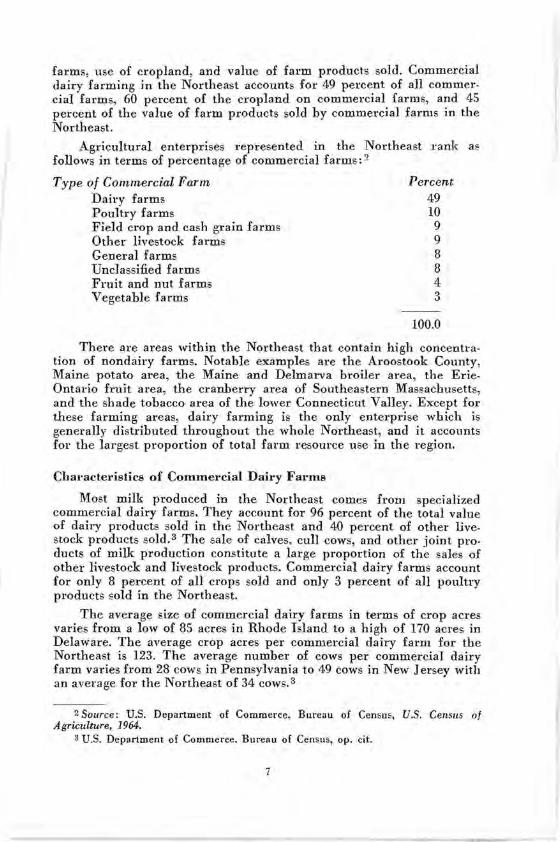
farms , use of cropland, and value of farm products sold. Commercial dairy farming in the Northeast accounts for 49 percent of all commer­cial farms, 60 percent of the cropland on commercial farms, and 45 percent of the value of farm products sold by commercial farms in the Northeast.

Agricultural enterprises represented in the Northeast rank a5 follows in terms of percentage of commercial farms: 2

Type of Commercial Farm Dairy farms Poultry farms Field crop and cash grain farms Other livestock farms General farms Unclassified farms Fruit and nut farms Vegetable farms

Percent 49 10 9 9 8 8 4 3

100.0

There are areas within the Northeast that contain high concentra­tion of nondairy farms. Notable examples are the Aroostook County, Maine potato area, the Maine and Delmarva broiler area, the Erie­Ontario fruit area, the cranberry area of Southeastern Massachusetts, and the shade tobacco area of the lower Connecticut Valley. Except for these farming areas, dairy farming is the only enterprise which is generally distributed throughout the whole Northeast, and it accounts for the largest proportion of total farm resource use in the region.

Characteristics of Commercial Dairy Farms

Most milk produced in the Northeast comes from specialized co=ercial dairy farms. They account for 96 percent of the total value of dairy products sold in the Northeast and 40 percent of other live­stock products sold. 3 The sale of calves, cull cows, and other joint pro­ducts of milk production constitute a large proportion of the sales of other livestock and livestock products. Commercial dairy farms account for only 8 percent of all crops sold and only 3 percent of all poultry products sold in the Northeast.

The average size of commercial dairy farms in terms of crop acres varies from a low of 85 acres in Rhode Island to a high of 170 acres in Delaware. The average crop acres per co=ercial dairy farm for the Northeast is 123. The average number of cows per commercial dairy farm varies from 28 cows in Pennsylvania to 49 cows in New Jersey with an average for the Northeast of 34 cows. 3

2 Source: U.S. Department of Commerce, Bureau of Census, U.S. CenSlLS of Agriculture, 1964.

3 U.S. Department of Commerce. Bureau of Census, op. cit.

7

Table 1. Total Milk Production, Number of Cows on Farms, and Milk Production per Cow, Northeast Dairy Area, 1956·1966"

1956 1957 1958 1959 1960 1961 1962 1963 1964 1965 1966

Total milk production in million pounds

23,919 23,485 23,705 23,763 24,566 25,274 25,504 25,655 25,747 25,703 24,903

Milk cows on farms in thousands

3,415 3,327 3,241 3,110 3,106 3,101 3,071 2,981 2,898 2,798 2,654

Milk production per cow in pounds

7,0'04 7,059 7,314 7,641 7,909 8,150 8,305 8,606 8,884 9,186 9,383

* Milk Production, Disposition, and Income, U. S. Department of Agriculture, Statistical Reporting Service, Crop Reporting Board, Washington, D. C.

Total milk production in the Northeast increased steadily from 1957 through 1964. The year 1965 marked the first time in eight years that there was a drop in total production. Yet during the period 1957·66 total milk production increased by 6 percent. 4 Over this period cow numbers dropped by 20 percent. Milk produced per cow increased by 33 percent. These changes reflect improvements in the technology of dairy production. The increase in output per cow is the result of better herd management, improvements in forage quality, increased concen· trate feeding, and closer culling of herds, as well as improvements in the genetic base of dairy cows.

Other changes in technology which have occurred include the con­tinued substitution of capital for labor through use of mechanical feed, manure, and milk-handling equipment. Greater use of new varieties of hybrid corn and improved hay species also characterize the technologi­cal change on Northeast dairy farms.

Market Structure and Pricing

The market structure of the eleven Northeastern States is dominated by six large Federal Order markets. These six markets serve approxi­mately 80 percent of the population of the region. Several States in the Northeast have State milk control boards or commissions which are functionally integrated with the Federal Orders for pricing to the pro­ducer. The actual level of prices is determined in various ways in the several marketing orders. Generally, the fluid use price is based on sev­eral economic indexes as well as supply-demand criteria. The nonfluid use is often tied to the average United States price for manufacturing milk and the butter price. Prices of the several classes of milk are usually the same in overlapped Federal and State market regions. But since the utilization rates for the various classes may differ between State and Federal destinations, the blend price paid farmers often differs between destinations.

The Federal and State milk orders in the Northeast impose an

4 See Table 1 and Figure 1.

8

25,500

s. ~

Million Ib

25,000 frJ ~ I----

.Q 24,500

7 U -5 24,000 o

~ 0:: ->< 23,500

(J)

E '­o

LL

c o (J)

~ o t)

== ~

~ o t)

.... Q)

a. c .9 u ::> '0 o 0:: ~

23,000

'F o

1956 '57 '58 '59 '60 '61 '62. '63 '64 '65 '66

Thousa nds

3600

t-0 N",

3400

3200

3000

2800

2600 ~i=

o

Lbs

9500

9000

8500

8000

7500

fHd , , , , , , , , , ,

1956 57 58 59 60 61 62 63 64 65 66

~ J--(

Vi ~

;t-j J 7000

1956 '57 '58 '59 '60 '61 '62 '63 '64 '65 '66

Years Figure 1. Total Milk Production, Milk Cows on Farms,

Milk Production per Cow, Northeast 1956.1966

9

*

*

:

institutional framework on the movement of milk inta and within the region. Changes in market area or source of supply come slowly but this stability is apparently desired by the industry.

Consumption and Utilization

The Northeast is a deficit area in terms of total milk supply. The production of fluid milk is generally adequate to satisfy consumption and no inshipments are made. Much of the supply of manufactured milk products, however, is shipped into the Northeast. Many of the products presently utilized by consumers could not originate in the Northeast since there are limited processing facilities in the area. Table 2 con­tains estimates of production and utilization of milk in the Northeast for 1965. These data illustrate the current requirements for inshipment of manufactured milk products in whole milk equivalents.

Item

Table 2. Estimated Milk Marketings, Utilization, and Net Inshipments, Northeast, 1965

Milk utilization Fluid Manufacturing

Total*

Northeast milk marketings and home consumptionT

Net inshipments of manufacturing and fluid milk

Pounds

(millions)

16,735 21,980

38,715

25,371

13,344

"See estimates developed for use by Hsiao, J. C. and Kottke, M. W., Spatial Equilibrium Arwlysis of the Dairy Industry in the Northeast Region - An Appli. cation of Qnadratic Programming, Storrs (Conn.) Agr. Expt. Sta. Bul. (in process).

t Milk Production, Disposition, and Income, 1965-66, Da 1·2 (67), Crop Report Board, SRS, USDA. (Combined marketings of milk and cream and milk used for milk, cream, and butter on farms where produced.)

Methodology for Estimating Supply Functions

There has been much discussion about the appropriate methods for estimating supply functions. The various approaches are well documented in the literature.5 The two techniques most commonly used to estimate supply are: (1) the regression of time series data, and (2) budgeting or linear programming. The regression approach is currently

5 See Earl O. Heady et. aI., Ed. Agricultural Supply Functions, Iowa State Press, Ames, 1961, or Marc Nerlove & K. L. Bachman, "The Analysis of Changes in Agricul· tural Supply: Problems & Approaches," Journal of Farm Economics, XLII pp. 531· 554, August 1960.

10

used principally in the analysis of short-run supply response. 6 In recent regional adjustment studies conducted in cooperation with the USDA, supply functions have been estimated through linear programming. The procedure is described briefly as follows:

(1) Stratify the region into areas based upon production oppor­tunities and natural resources.

(2) Sample each area to provide a basis for constructing represen­tative farms.

(3) Construct representative farm linear programming models and solve them with a series of product prices to obtain step supply functions.

(4) Sum the supply functions of the individual representative farms over areas or regions.

This section describes each of the above steps. The procedures employed in this study are for the most part similar to those used in the other regional adjustment studies. A notable exception is the meth­od adopted for the specification of representative farms which is de­signed to reduce bias in the aggregation of supply functions.

Selection of Areas Within the Northeast

The objective of stratification is to divide the region into farming areas that are homogeneous in terms of such factors as climate, topo­graphy, soils, or marketing outlets. Thus, the farms within the area might be expected to have the choice of similar enterprise alternatives, and to be faced with similar yield potentials, prices, and costs. The stratification of the region into areas is followed by the classification of all farms into a smaller number of representative farm groupings within areas. The task of selecting areas and representative farms within areas is closely related.

The Northeast region was divided into 20 such areas based upon the ahove considerations. These areas are shown in Figure 2 and are identi. fied as follows: 7

1. Central Maine 2. Southern Maine-Southern New Hampshire 3. Southeastern New England 4. Northeastern Vermont-Northwestern New Hampshire 5. Southeastern Vermont-Southwestern New Hampshire 6. Southwestern New England 7. Northwestern Vermont 8. Southwestern Vermont 9. Hudson Valley

10. Northern New York 11. Oneida, Mohawk, and Black River Valleys

6 Effort has been made by Nerlove and others to estimate long-run supply elasti. cities using time series analysis_ See Marc Nerlove, The Dynamics of Supply, tbe John Hopkins Press, Baltimore, 1958_

7 Urban centers and forest or mountain lands are not considered as production areas.

11

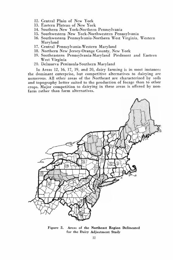
12. Central Plain of New York 13. Eastern Plateau of New York 14. Southern New York-Northern Pennsylvania 15. Southwestern New York-Northwestern Pennsylvania 16. Southwestern Pennsylvania· Northern West Virginia, Western

Maryland 17. Central Pennsylvania-Western Maryland 18. Northern New Jersey-Orange County, New York 19. Southeastern Pennsylvania-Maryland Piedmont and Eastern

West Virginia 20. Delmarva Peninsula·Southern Maryland

III Areas 12, 16, 17, 19, and 20, dairy farming is in most instances the dominant enterprise, hut competitive alternatives to dairying are numerous. All other areas of the Northeast are characterized by soils and topography better suited to the production of fOL·age than to other crops. Major competition to dairying in these areas is offered by non­farm rather than farm alternatives.

Figure 2. Areas of the Northeast Region Delineated for the Dairy Adjustment Study

12

Farm Sample and Sampling Procedure

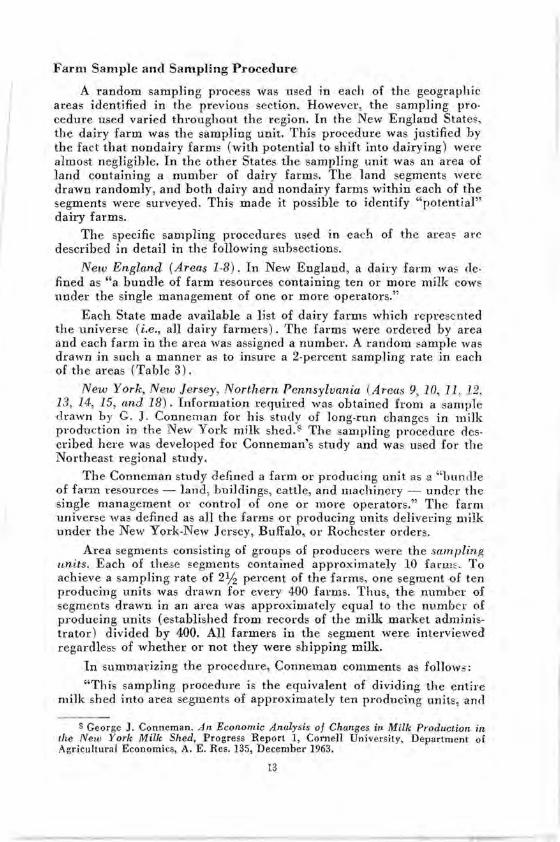
A random sampling process was used in each of the geographic areas identified in the previous section. However, the sampling pro­cedure used varied throughout the region. In the New England States, the dairy farm was the sampling unit. This procedure was justified by the fact that nondairy farms (with potential to shift into dairying) were almost negligible. In the other States the sampling unit was an area of land containing a number of dairy farms. The land segments were drawn randomly, and both dairy and nondairy farms within each of the segments were surveyed. This made it possible to identify "potential" dairy farms.

The specific sampling procedures used in each of the area~ are described in detail in the following subsections.

New England (Areas 1-8). In New England, a dairy farm was de­fined as "a bundle of farm resources containing ten or more milk cows nnder the single management of one or more operators."

Each State made available a list of dairy farms which represented the universe (i.e., all dairy farmers). The farms were ordered by area and each farm in the area was assigned a number. A random sample was drawn in such a manner as to insure a 2-percent sampling rate in each of the areas (Table 3) .

New York, New Jersey, Northern Pennsylvania (Areas 9, 10, 11 , 12, 13, 14, 15, and 18). Information required was obtained from a sample drawn by G. J. Conneman for his stndy of long-run changes in milk production in the New York milk shed. 8 The sampling procedure des­cribed here was developed for Conneman's study and was used for the Northeast regional study.

The Conncman study defined a farm or producing unit as a "bnndJe of farm resources - land, buildings, cattle, and machinery - under the single management or control of one or more operators." The farm universe was defined as all the farms or producing units delivering milk under the New York-New Jersey, Buffalo, or Rochester orders.

Area segments consisting of groups of producers were the sampling units. Each of these segments contained approximately 10 farm~ . To achieve a sampling rate of 2Yz percent of the farms, one segment of ten producing units was drawn for every 400 farms. Thus, the number of segments drawn in an area was approximately equal to the number of producing units (established from records of the milk market adminis­trator) divided by 400. All farmers in the segment were interviewed regardless of whether or not they were shipping milk.

In summarizing the procedure, Conneman comments as follow3:

"This sampling procedure is the equivalent of dividing the entire milk shed into area segments of approximately ten producing units, and

S George J. Conneman, An Economic Analysis of Changes in Milk Production in rhe New York Milk Shed, Progress Report 1, Cornell University, Department of Agricultural Economics, A. E. Res. 135, December 1963.

13

selecting the appropriate number of segments by a chance procedure that insured geogt'aphic distribution of the segments."9

Pennsylvania, Maryland, Delaware, and West Virginia (Areas 15, 16,17,19,20). The producing [init was a farm classified by census defin· ition. The universe of farms consisted of dairy, live · tock, and crop farms, with the exception of specialized fruit, vegetable, and poultry farms. The number of farms (other than specialized) was determined for each township from the 1959 census. The sampling unit consisted of a town· ship, or portion thereof, containing more than 10 farms hut less than 30 dairy or potential dairy farms. Ideally each segment would consist of 20 farms. However , segments of farms were formed on a township basis because this was the smallest geographical un'it for which the number of farms could be estimated. No segments cut across township lines

Sampling units or segments were grouped into blocks. A block con· sisted of 800 farms in AJ:ea 15, 1,000 farms in Areas 16 and 17, and 1,333 farms in Area 19. A bJock in Area 16 would contain 50 segments

Table 3. Total Dairy and Potential Dairy Farms, Sample Rate and Number of Farms Sampled by Area and State for the Northeas t, 196'0

Number of Percent Total Area Stnte sample farm s sample rate farms

l Me. 57 2.0 2,910 2 Me., N.H. 51 3.5 1,473 '1 l\l ~ss., R.I., Ct. 94 U 2,995 4- Vl. 39 2.1 1,859

N.H. 7 3A 208 Vt. 23 2.4 968 N.H. 13 2.9 619

6 Mass. 34 2.9 1,168 Ct. 36 2.7 1,317

7 Vt. 71 3.2 2,22<1. R Vt. 19 3.1 61~ 9 N Y. 192 3.9 4,960

10 N.Y. 147 2.5 5,880 11 N.Y. 182 2.5 7,280 J2 N.Y. 157 25 6.280 F N.Y. 225 2.5 9,000 oj

14 N.Y. 85 2.5 3,400 Pa. 164 2.6 6,43J

15 NY 88 2.5 3,520 Pn. 100 2.4 4·.219

16 P:l . 271 3.~ 8,931 17 Pa. 164 1.7 9.1i<17 13 N.J. 77 2.5 3,080 19 Pa. 258 1.7 15.460

Md. 73 1.4 5,196 20 Md. 75 3.6 2.058

Del. 32 ].0 3,292

Total . Northeast 2,739 2.4 Jl4,990

n Ibi d.

J4.

(50 x 20 = 1,000). Sample segments were drawn randomly from within blocks. Therefore, the construction of blocks within areas provided a further guarantee of uniform geographic distribution of segments. The sampling rate varied between areas, being 2Vz percent in Area 15,2 per­cent in Area 16 and 17, and IVz percent in Area 19.

Farm Survey Data

Farms in the samples were surveyed in the summer of 1961. A total of 2,739 schedules were usable for analysis. The survey was designed to obtain information to permit a description of the resources available for use by the individual farmer. Data were collected regarding cropland and its use, the capacity and use of farm facilities, labor supply, and capital structure. In addition, information was obtained concerning pro­duction practices. The survey data provided the basis for developing representative farm models.

Other Data

To complement the farm survey data, production, cost, and price data were assembled from secondary sources.1 o These provided a con­sistent basis for developing model coefficients which reflect the real difference in the productivity of resources and price differences be­tween the 20 areas studied. Two sets of production relationships were specified. An average set of coefficients was established representing yields with average management and technology used in 1960-61. In addition, a similar set of coefficients was developed representing manage­ment and yields associated with the top 25 percent of farmers in 1960-61. These superior production relationships were used III the analysis done in this study.

Long-term real estate credit borrowing capacities had to be de­veloped. The survey schedules provided information concerning farm debt. Real estate appraisals of representative farms by areas were made by members of the Farmers Home Administration. Net worths for study farms were then calculated and borrowing capacities computed.

The price projections used in the Lake States Dairy Adjustment Study provided the basis for the level of prices.1 1 Historical price rela­tionships were investigated for each of the 20 areas in the Northeast. Since the milk price was varied in the linear pl'ogramming analysis, this was the only historical price that was not built into the analysis. Input costs whose levels were not specified were estimated to correspond with the regional price relationship of other items. The intent of these pricing procedures was to simulate historical relationships at an expected 1965 level.

10 Agriculwral Planning Data for the Northeastern United States, Pa. Agl-. Expt. Sta., A.E. & R.S. 51, July 1965_

11 Sundquist, W. B., et. al., Equilibrium Analysis of Income - Improving ad­justments on Farms in the Lake States Dairy Region_ Minn. Agr. Expt. Sta. Tech. Bul. 246, 1963.

15

Method of Developing Representative Farms

The research procedure used in this study consists of defining a universe of farms, selecting a number of benchmark farms to repre· sent the universe, and developing optimum plans for these farms at variable commodity prices by linear programming. The programmed results are expanded to obtain an aggregate supply response for the universe. The difference between the aggregate supply response oh· tained by this procedure and one obtaineed by programming all farms is defined as aggregation bias.

A considerable effort was made to minimize the bias in the supply estimation that could be attributetd to aggregation of benchmark farm data. In the past, the selection of benchmark farms has been done rather arJ)itrarily, usually on the basis of some common size measure. This procedure, which is done without regard to the relative level of reo sources on the farms, gives rise to a considerable upward bias in the supply response. This can be easily demonstrated. If farms are c1a,si· fied on the basis of the lahor resource, any resulting subgroup may contain some farms that are scarce in labor but have surplus capital, and others on which the resource situation is reversed. Whcn the reo sources of such farms are averaged, the disproportionalities existing on individual farms tend to be averaged out. Thus, the conventional bench· mark will not reflect the restrictive resources of the individual farm ;;, and its expanded output overestimates the aggregate outpnt. 12

Representative farms were constructed on the basis of estimated homogeneous restrictions,13 Sample farms from the surveys were group· ed according to their most limiting resource in the linear programming model and benchmark farms were defined as the average of resources on all farms within each group. This procedure differs from more con· ventional methods of representative benchmark farm selection in that it takes into consideration the relative availability of resources and the productivity of resources. Usually fanns are classified on the basis of the absolute magnitude of certain resonrces snch as cropland, labor, and number of livestock. The homogeneous restriction method of represen· tative farm selection was used because the supply response of milk based on the farms selected by this method contained a minimum of aggregation bias.

12 Frick, C. E. and Andrews, R. A., "Aggregation Bias and Foul' Metbods of Summing Falm Supply Functions," Journal of Farm Economics, Vol. 4·7, No.3, Pp. 696·700, August 1965.

13 For a detailed discussion of tbis technique, see Se?mus J. Sheehy, "Selection of Representative Benchmark Farms in Synthetic Supply Estimation," Ph.D. Thesis, Pennsylvania State University, August 1964; Seamus J. Sheehy and R. H. McAlex· ander, "Selection of Representative Benchmark Farms for Supply Estimation," Journal of Farm Economics, Vol. 47, No.3, Pp. 681.695, August 1965. Also R. Barker and B. F. Stanton, "Estimation and Aggregation of Firm Supply Functions," Journal of Farm Economics, Vol. 47, No.3, Pp. 701·712, August 1965.

16

Grouping of Farms

Surveyed farms were grouped into six different homogeneous re­striction classes for determining benchmark farms. Previous work in­dicated that a more detailed grouping of farms on the basis of homo­geneous restrictions gave only slightly different aggregate supply func­tions, but the magnitude of the programming time was considerably greater.

In selecting representative dairy farms, some assumptions lvere made as to how a dairy farm could be defined. In this study it was as­sumed that any farm selling milk at the time of the survey would be considered a dairy farm. If milk were not being sold from a farm at the time of the survey, such a farm could be considered as a potential dairy farm if it had resources for at least 20 cows. Farms without sufficient resources for at least 20 cows were not included in the programming phase of the analysis.

The six farm groupings were as follows: Group 1: Nondairy farms, or those with resources for less than 20

dairy cows. Group 2: Dairy and potential dairy farms on which the forage

supply was estimated to permit fewer cows than the winter labor supply or existing dairy building capacity.

Group 3: Dairy and potential dairy farms on which the forage supply was estimated to permit fewer cows than the winter labor supply or total dairy building capacity (existing capacity plus added space permitted by ex­pansion with real estate mortgages), but more cows than with existing dairy building capacity.

Group 4: Dairy and potential dairy farms on which winter labor was estimated to permit fewer cows than the forage supply or the existing dairy building capacity.

Group 5: Dairy and potential dairy farms on which winter labor was estimated to permit fewer cows than the forage supply or the total dairy building capacity, but more than the existing dairy building capacity.

Group 6: Dairy and potential dairy farms on which total dairy building capacity was estimated to permit fewer cows than the forage supply or winter labor supply.

The procedure for grouping of selected farms can be illustrated by the data in Table 4. Information is given on cropland, permanent pas­ture, soil capacity, dairy building capacity, borrowing capacity, and the winter labor supply on six sample farms for a particular area in the study. This information, along with requirements of dairy cows for these items, provides a basis for classifying each of the farms into groups 1 through 6.

Farm 1 in Table 4 represents a nondairy farm in that the numher of cows based on (1) the forage supply that could be produced on the land (Row 8) , (2 ) the winter labor supply (Row 9), or (3) dairy barn

17

expansion based on loan value of real estate along with the present dairy barn capacity (Row 10) was less than 20 cows. Thus, in accordance with the assumption that a dairy farm would not come into existence with less than 20 dairy cows, Farm 1 is classified as a nondairy farm and placed in Group l.

Examination of the number of dairy cows possible with the various resources on Farm 2 shows that the forage supply is the most limiting resource, permitting about 25 cows; whereas winter labor and existing dai1'Y huildings would permit approximately 62 and 31 cows, respec­tively. Thus, this farm would be placed in Group 2.

Table 4. Grouping of Selected Farms on Basis of Homogeneous Resources

Farms classed by homogeneous restriction method

Group Group Group Group Group Group Item 1 2 3 4 5 6

1. Cropland, acres" 59 51 60 49 78 65 2. Permanent pasture,

acres ~~ 8 23 10 25 30 ]4 3. Silo capacity, tons'" 90 80 60 70 60 4. Winter labor, hours';' 549 1841 1130 808 1126 1405 5. Borrowing capacityt 8178 9738 10616 9972 10500 0 6. Number additional cows

possible based on borrowing capacity+ 14.3 17.1 18.5 17.5 18.3 0

7_ Existing dairy capacity, number cows ": 0 31 27 23 28 20

8. Number cows possible with forage supply§ 27.8 24·.9 28.3 25.2 39.1 30.4

9. Number cows possible with winter labor supplyll 12.4 6l.7 34,5 22.3 31.0 45.0

10. Number cows possible with ex isting plus added dairy barn capacityff 14.3 48.1 45.5 40.5 46.3 20

" Based on information obtained from the operator. t Borrowing capacity is based on 50 percent of owned estimated real estate value

less existing mortgages. t Based on borrowing capital divided by S571, the estimated cost of adding

building space for the dairy cow and one-fourth replacement. ' § Based On a rotation and forage requirement of dairy animals requiring for

each cow and one-fourth replacement, 2.5 acres of cropland, or 5.1 acres of permanent pasture, or 35 tons of silage capacity.

II Based on an estimated labor requirement of 26.2 hours of winter labor per cow and one·fonrth replacement and 225 hours of fixed dairy labor during this period.

ff Based on the number of cows permitted with existing dairy building space (Row 7), plus additional cows possible with borrowed funds (Row 6).

NOTE: The resource quantities shown are merely examples for selected firms in one area of the study. The coefficients used in computing the numher of cows (including one-fourth replacement for each cow) could differ by areas due to such differences as crop yields, types of forages, length of forage stand, fertilization levels, forage·grain substitutes in the dairy ration, Or differ· ences in length of the winter season when estimating total quantity of winter labor.

18

The estimation of the number of cows permitted by the foragc supply is somewhat more cumbersome than for other resources. The forage supply depends upon such factors as the type of forage produced, length of stand, level of fertilization, as well as the possible substitu­tion of forage for grain in the dairy cow ration. Estimation of the most likely forage supply for farms with alternative resource bases can be made by some preliminary programming and determining the types of results obtained. By varying cropland, rather close estimates of forage production and utilization are possible for farms with different resource combinations.

Farms 3 through 6 have been classified into Groups 3, 4, 5, and 6, respectively. Farm 3 would be limited to 28 cows by the forage supply, with cow numbers above that of existing dairy barn capacity but less than total dairy building capacity. Farm 4 would he limited to about 22 cows by the quantity of winter labor, which is less than the existing dairy barn capacity and the forage capacity on this farm. Farm 5 would have enough winter labor for 34 cows, which would allow six more cows that the present dairy building capacity but fewer cows than the forage supply or the total dairy building capacity. Farm 6 would be limited to 20 cows hy the total dairy barn capacity, or fewer cows than permitted by the winter labor or forage supplies on this farm.

The farms in differcnt States were classified in this manner. There were variations in such items as length of winter season, yields, and value of property between many areas, resulting in different coefficients than those used for the computations in Table 4. Also, some researchers first classified farm by size of dairy herd before grouping according to the most limiting resource.

Development of Restrictions and Machinery Complements

After the farms were classified, a single benchmark farm was selected for each group excluding the nondairy group. Resource re­strictions were then developed for the bcnchmark farm which were merely averages of the farms within each group. For example, averages were computed for acreages of cropland and permanent pasture, tons of silo capacity, borrowing capacity, and existing dairy housing space. In developing the machinery complements for each benchmark farm, the model incidence on farms in each group was used.

The Linear Programming Models

Linear programming models were designed to compute the opti­mum organization of representative farms from the standpoint of max­imizing profits. Implicit in the construction of the models was the hypothesis that farmers adjust output in response to prevailing milk prices, factor costs, and the state of technology, so as to maximize re­turns from available labor, land, and capital resources. The lineal' pro­gramming models were coordinated with respect to four major con-

19

siderations: (1) the comparability of models for the various areas, (2) the choice of production activities, (3) the extent of resource con· straints, and (4.) the price variability among areas.

Comparability of Models for the Various Areas

The general stmcture of dairy farms throughout the Northeast region appeared to be sufficiently alike to warrant basically similar linear programming models for all areas. However, each participating state developed its own model so that unique characteristics of each area could be reflected. As a consequence, the various models have spme identical equations and some modifications to fit particular area situa­tions. Special care was taken to insure that intraregional productivity differences, if any, would be manifested in the results. All input-output data were carefully scrutinized for intraregional consistency and com­parability. Differences in results among areas, therefore, represent the prevailing conditions of each area rather than differences in procedures and assumptions.

Choice of Production Activities

Conditions that usually guide the selection of actIvItIes ff)r linear programming models are: (1) the relevant time period, (2) the state of technology, and (3) the degree of specialization.

In this study the problem was to develop a model which was to maximize profits allowing resource use changes and additions that could occur within intermediate run conditions. This temporal condition dic­tated models designed to depict the pmduction choices available to fariners if they had sufficient time to adjust feeding rates and milk yields, fertilizer rates and crop yields, crop selection and hay procurement methods, dairy cow replacement methods, seasonal labor employment, and barn capacity and silo capacity. Certain areas, in addition, permitted choices lJetween dairy and other livestock enterprises, principally beef and hogs. In calendar time, the study specified 1960 as the base year and initially set 1965 as the target date. 14

The input-output coefficients used in the model reflect the temporal nature of the problem. Coefficients were used representing management and yields associated with the top 25 percent of the farmers in 1960·61. These relationships were considered to be representative of aggregate farmer response within the time span of the model.

Since most of the New England dairy fanners have few farm enter­prise alternatives, the activities for New England models represented specialization in the dairy enterprise. Some diversification is represented by activities included in the models for the other areas of the North­east. For example, the New York and Pennsylvania models included

14 The in('ome results of the models are for a single year's operation. Each sd­justment and its corresponding income is considered as a single adjustment to reach static equilibrium, while some activities would likely require several years to reach this equilibrium.

20

grain production actlvltles besides the beef and hog enterpri£es men­tioned previously.

Extent of Resource Constraints

The major constraints in the model were those pertammg to the representative farm's land, labor, and capital resources. It was assumed for the intermediate run conditions that the farm's 1960 inventory of land could not he expanded. The reason for constraining the land rc­sources of the representative farm to those that existed in 1960 was that while land supply of an individual farm is not actually fixed, the aggre­gate supply for- the region is fixed. From a methodological standpoint, it was requisite to constrain land supply of the individual farm to insure the fixed land supply of the region.

Five labor constraint equations were used; one was for each of fonr seasonal periods and one for regular hired labor. Full-time hired labor and seasonal labor could be hired in the models.

Winter lahor was constrained to that available in the form of the op­erator's family labor and the regular full·time hired labor on representa­tive farms as of 1960.

A reservation price was placed on the available family labor to reflect the condition that a farmer may not be willing to spend time on some marginal activities unless the return was great enough to cover a minimal reward for this effort.

Funds for capital expansion were constrained to 50 percent of the farm's 1960 real estate value, minus the 1960 outstanding debt.1 5 These capital funds could be used for barn and silo expansion. The model was designed to permit expansion in cow carrying capacities of a farm, but limited to an investment ceiling which reflected the credit base of the farm. Funds for annual production were not limited; however, an annual return of 6 percent was required on all production investment capital.

Variable Prices

Two considerations were confronted in regard to price variation. Should only the price of milk vary with all other prices assumed constant, or should other prices vary also? What is an appropriate range of price variation? On the first question, it was decided to variable­price program by varying only the price of milk. For the second ques­tion, solutions were obtained for the $2.80 to $6.40 per hundredweight range in milk price.

15 Tbe survey schedules provided information concerning farm debt. Real estate appraisals of representative farms by areas were made by members of the Farmers Home Administration. Net worths for study farms were then calculated and borrow­ing capacities computed. If it were determined that a particular farm had a negative borrowing capacity, it was rounded up to zero.

21

Table 5. Abbreviated Tahleau of the Linear Progl'ammillg Model Used for Area :V

C - c --e - c - c - c c -c -c -c

Activities <n <n ." ~ .,; ., ... ,<

Constraints,

~ 0 ;]-

<n

~ Q. <:

'" '" " -'" .= '" 0 0

"" " ,

controls, '" ~ '" ;:; '" 0 ., ..... - '" .0'" ., 'w :>, '" C; " ,.

and transfers '" :0 0;:: 0 ~() 0 '" 0

"' '" " e " '" '" '-' J == " "' C,~ '-' ~

."::: :.... !" ..<: .s: bJJ " ., '" ~'tJ X " ';: :>, "' ., :>, "0 ",,0 ., '" >-..... <n '" <:

.~ ~J ..... ;>. '" ;;; <i ..,.. 01 '" " " " ~;;; '" "" "0.0 C <l " '" <l ~ CO ;> ""~ :0 :0 -<e -<e:; ... , lfl :0 0:: "" Z lfl

13 3 '1·,9 ]0 11-14 15 16-17 18-21 22 23 24 25 26-39 40-41 42

Milk transfers I -a .., F eed·cow trans, 2 - I - I I .., Crop acres 3-6 h a a

Forage transfer 7 -a -I -a Pasture control 8-10 - 3 -a a Grain tran5fer 11 -I a Hay transfer 12 3 -a - 3

-M Base cows B h Cows 011 hand 14- II - I Barn capacity 15 h a - I Repl. control 16-l8 h Hay control 19-20 +3 -i.(l a -3

Silo capacity 21 h -1 3

Labor by <ltrs. 22-26 b a " a -a a a Seeding control 27-28 a -a Cash reservation 29 a a a -a a a Capital funds 30 b a

" In tbis condensed form the elements only suggest the general relation of "cti,'ities and com,traints. Since some of the ro"" and columns are combined, some of the elements designated "a" or " .,," may rep resent severa l elcme nt" The clement;; des igna ted ~'*" represen t a CO lnhination of positive and negativ e c lcme nt ~ .

A Linear Programming Model for One of the Representative Farms

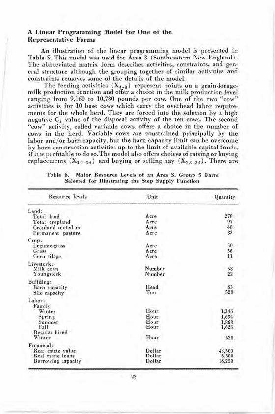
An illustration of the linear programming model is presented in Table 5. This model was used for Area 3 (Southeastern New England) . The abbreviated matrix form describes activities, constraints, and gen· eral structure although the grouping together of similar activities and constraints removes some of the details of the model.

The feeding activities (X4 - 9 ) represent points on a grain·forage· milk production function and offer a choice in the milk production level ranging from 9,160 to 10,780 pounds per cow. One of the two "cow" activities is for 10 base cows which carry the overhead labor require­ments for the whole herd. They are forced into the solution by a high negative C i value of the disposal activity of the ten cows. The second "cow" activity, called variable cows, offers a choice in the number of cows in the herd. Variable cows are constrained principally by the labor and/ or barn capacity, but the barn capacity limit can be overcome by barn construction activities up to the limit of available capital funds, if it is profitahle to do so. The model also offers choices of raising or buying replacements (Xl 0 -14) and buying or selling hay (X2 3 -2 '1)' There are

TaLle 6. Major Resource Levels of an Area 3 , Group 5 Farm Selected for Illustrating the Step Supply Function

Resource levels Unit Quantity

Land: Total land Acre 278 Total cropland Acre 97 Cropland rented in Acre 48 Permanent pasture Acre 83

Crop: Legume-grass Acre 30 Gra ss Acre 56 Corn ,i1age Acre 11

Livestock: Milk cows Number 58 Youngstock Number 22

Building: Barn capacity Head 63 Silo capacity Ton 528

Labor: Family

Winter Hour 1,346 Spring Hour 1,634 Summer Hour 1,868 Fall Hour 1,623

Regular hired Winter Hour 528

Financial: Real estate value Dollar 43,5()0 Real estate loans Dollar 5,500 Borrowing capacity Dollar 16,250

23

seventeen forage-producing actIvItIes (X2 5 -39) and (X40 - H ) offering selections of corn silage at two fertilizer rates, alfalfa hay at two lengths of stand and two fertilizer rates, clover grass at two fertilizer rates, mixed grass at two fertilizer rates, and two lengths of stand and perm­inent pasture at two fertilizer rates.

Altogether, the model offers numerous possibilities of different combinations of inputs and outputs that Area 3 dairy farmers typically would face under the intermediate run conditions of this study.

Table 7. Milk Supply Function, Area 3 Representative Farm, Group 5

Price Optimum Annual grain Dairy cow of milk milk output Number feeding level replacement per cwt. in cwl. of cows in pounds program

$2.30 3866 42 1500 raise, sell 3.01 4050 44 1500 raise, sell 3.19 4299 47 15'00 raise, sell 3.20 4423 48 1500 raise, sell 3.41 4906 54 1500 raise, sell

3.46 5037 55 1500 raise 3.50 5074 55 15'00 raise 3.74 5187 55 1750 raise ~.78 5371 56 1750 raise, buy 3.83 5442 57 2000 raise, buy

4.02 5563 58 2000 raise, buy 4.03 5577 58 2000 raise, buy 4.15 6'057 58 2000 raise, buy 4.48 6291 63 2000 raise. buy 4.49 6300 63 2000 raise, buy

5.02 6305 63 2500 raise, buy 5.03 7090 71 2500 buy 5.19 7500 73 3'000 buy 5.21 7773 75 3000 buy 5.42 9158 89 3000 buy

5.46 9221 89 3000 buy 5.71 9775 92 3500 buy 6.o? 10017 94 3750 buy 6.45 10120 94 375'0 buy 6.50 10120 94 3750 buy

Linear Programming Solutions for a Representative Farm

A representative farm from Area 3, in this case one in the Group 5 category, with resources such that winter labor is the most effective constraint, can illustrate the model. As surveyed, the dairy herd had 58 cows which made it about 20 cows above average size for Area 3. The major resources of the farm are shown in Table 6. The variable­price programming resulted in a range of optimal annual milk out­puts from 386,600 to 1,012,000 pounds (Table 7). In general, milk prices below $3.40 per hundredweight have optimized solutions in­volving less than 50 cows, the lowest grain feeding level, the sale of

24

some hay, and the sale of some replacement stock. At milk prices be­tween $3.40 and $4.40, the solutions indicate 58 cows (the representa­tive farm's 1960 number of cows on hand), the second lowest grain feeding rate and the raising of replacements_ If milk price ranges be­tween 34.40 and $5.00 per hundredweight, the farm should operate at full barn capacity (63 cows). As the price gets higher, the optimized solutions call for significant adjustments in the farm's operations. Ex­pansion of barn facilities to permit up to 94 cows, increase in feeding rates to the highest levels, and a change to a "purchase replacements" program are indicated. The nature of the step supply function suggests that this farm should be relatively sensitive to price changes under intermediate run conditions (Figure 3) . The implication of the function is that the potential milk supply forthcoming from the representative farm of Area 3 at a price, say $5.20, should be about 44,000 pounds greater than if the price were $1.00 less and the price of milk and prices of other factors were expected to hold long enough for the inter­mediate run conditions to prevail.

Pric e per cwt.

I( $7.0

I( 6.0 '-

5.0 ~

0 .r-

~ 4.0

3.00

2.00

~ o 3,000 4,000 5,000 6,000 7,000 8,000 9,000 10,000

Optimum Milk Output in Cwt.

Figure 3. Milk Supply Function, Area 3 Farm, Group 5 Category

2S

summation of these two linear demand functions. The resulting demand functions are shown in Figure 5. By horizontally summing these two demand functions, the classified pricing provisions are neglected and a single price for both fluid and manufacturing milk is assumed. This assumption is not representative of the market in the Northeast.

Regional Price-Quantity Disappearance Curve Under Classified Pl'icing

Where most milk produced and sold in the Northeast is inclmlelJ nndel' either a Federal or State market order, a price-quantitv relation­ship reflecting this market structure would be more meaningfnl than the combined linear demand function.

A price· quantity relation which reflects the existing cla3s ified pric­ing system was developed_ The regional demand function for fluid milk was used to represent the demand for fluid milk for the region. An infinitely elastic demand curve was assumed for manufacturing milk. In othet· words, an unlimited quantity of milk could be sold at the manufacturing price and the quantity of manufacturing milk pro­duced in the Northeast would have no influence on its price.

Under the classified pricing structure there exists a demand func­tion similar to that assumed for fluid mille A price for fluid lllilk is H" t

in each market under the market order by a milk control board (or a ~ determined at hearings or some method of formula pricing) . Hence, the price paid farmers for fluid milk is determined by administrative decree. The quantity sold is determined by the quantity of milk consnmers are willing to purchase at this administratively estahlished price.

Support for a perfectly elastic demand for manufactured milk can be found in the performance of the manufactured milk market. Thi;­market is national in scope_ The Northeast supplies a very small portion of the total quantity. In fact, the Northeast is a substantial deficit area; it imports about one-third of the manufactured products (in whole milk equivalents) consumed. Thus, the Northeast output of manufacturer] milk has negligible influence on the price.

Two more points about the price of manufactnred milk shonld be made. First, the price of manufactured milk is also administratively determined in many Northeastern markets and is frequently haEed o~ the U.S. average manufacturing milk price. Second, the Federal Govern­ment price support activities for milk products effectively establishcs a pr!cc floor for manllfactured mille If the fluid demand a!1d manufactur· ing rlf'llland functions described above are evaluated using a milk price blend formula, a line resemhling ABC, Figure 6, can be traced. Curve ABC l'cprescnts the price that farmers would receive if various quan­tities of milk were produced.

I I I

The blend price formula was employed to determine the fluid milk price and utilization with the 1965 blend price, manufacturing price, the demand function for fluid milk, and total milk consumption. 2 5 The estimated price. quantity curve describes how prices received by farmers would vary as quantity of milk varies under the existing blend pricing system with the demand relationships of 1965.

Implications of the Price-Quantity Equilibrium

The fonr supply relations and two demand situations provide a total of eight price-quantity equilibrium situations to he analyzed. These eight price-quantity equilibrium components are shown in Figure 7 and Table 12. For comparison, the weighted average price and quan­tities produced in 1965 and the departures from each of the eight esti­mated equilibrium prices and quantities are included. The closest to 1965 is Equilibrium No.9, the one developed on the basis of the classified milk market structure with blend price relationship con­fronting farmers and a supply function that reflects the 1965 resource hase and transportation diffel'entials between the 20 areas in the Northeast.

Most outstanding in the analysis of the eight estimated equilibrium situations is the error in estimating quantity when supply functions were based upon the 1960 resonrce base. This error was sizable for both demand situations and both supply assumptions. See Equilibriums 2, 3, 6, and 7 in Table 12 and Figure 7. .

The use of the demand fnnction developed by linear summation also introduced a source of error. For example, Equilibriums 4 and 5 for supply function with the 1965 resource ,base in which the demand function assumes away classified pricing and inshipments of milk.

r,Q, + P2Q2 25 The standard blend price formula is: P

B Q, + Q2 However in developing the price-quantity di sappearance curve, P , P2, and

B Ql + Q2 are predetennined. The problem is to find the Class I Pri ce, PI , and Class I utilization, Q), such that the price-quantity disappear~nce 'curve will pass through the point.

Substituting the linear demand function relating Ql to P[, and solving by the binomial theorem yields:

Where:

-(a-bP2) +v(a-bP2)2 - 4hlP2Q - aP2-Q P

2h

PI = Price of Class I (fluid) milk P2 = Price of Class II (manufacturing) milk P = Blend price

B Ql = Quantity of milk for Class I (fluid) UEe

H

Q2 = Quantity of milk for Class II (manufacturing) use Ql + Q2=Total quantity of milk, Q

Ql = a + hPI = Demand function for Class I milk

37

Two major implications are observable from this analysis. (1) Changes in resource bases and shifts in technology, commonly called "short-run supply shifters," are more important in determining quan­tities supplied in the Northeast than is the elasticity of the supply functions as determined by this study. This is true even in the inter­mediate time period. The importance of a supply shifter is clearly seen in Figure 7 when the supply functions for the 1960 resource baEe are compared with the supply functions for the 1965 resource base. (2) The total supply potential for milk in the Northeast declined considerably between 1960 and 1965 due to the decline in the resource base. It is doubtful that new technology has been developed to offset this decline in potential due to loss in resource base. In spite of this, there exists a substantial potential for expansion in milk supply if all dairymen adopted the top 25 percent technology available to them in 1960.

-o Q)

o ....

0..

Blend

~ ~,""fo"",i" d,mo,d

Fluid demand

Quantity of Milk

Figure 6. Theoretical Fluid Demond, Manufacturing Demand, and Blend Price-Quantity Curve

38

c

Table 12. Summary of Regional Supply-Demand Relationships and Comparison with Actual 1965 Price and Disappearance

Demand situation Supply situation Departure from 1965

Price· Location Linear Quantity No area price With area price Equilibrium Price Quantity number on sum· disap· differentials differentials Figure 7 mati on pearance Resource base Resource base

Per· Per· 1960 1965 1960 1965 Price Quantity Actual cent Actual cent

C>.) (Mil. cwt.) (Mil. cwt.) "" 1 (1965

actual) 34.84 253.7 $.00 0.0 2 X X 4.20 378.0 - .64 -13 +124.3 +49 3 X X 4.30 374.0 -.54 -11 +12'0.3 +47 4 X X 5.42 338.0 +.58 +12 +84.3 +33 5 X X 5.46 336.0 +.62 +13 +82.3 +32 6 X X 4.28 384.0 -.56 -12 +130.3 +51 7 X X 4.32 376.0 -.52 -11 +122.3 +48 8 X X 4.55 309.0 -.29 -6 +55.3 +22 9 X X 4.58 302.0 -.26 -5 +48.3 +19

Appendix Table 2. Linear Programmed Milk Supply Functions, 20 Areas in the Nort11east with 1960 Resource Base,

No Area Price Differentials

Price Area 1 Area 2 Area 3 Area 4 Area 5 Area 6 Area 7 Area 8

Thousand cwt.

82.80 4,879 3,624 7,200 7,191 5,617 *6,380 9,048 2,649 3.20 5,834 3,910 7,871 8;024 5,734 *7,193 9,669 2,714 3.60 6,443 4,304 8,893 8,443 6,341 7,204 10,310 2,801 4.00 7,001 4,683 9,635 9,504 6,814 8,849 11,811 3,157 4.20 7,050 5,059 10,221 9,913 7,603 9,161 12,679 3,317

4.40 7,285 5,286 10,509 10,081 7,857 9,783 12,857 3,504 4.60 7,480 5,505 10,887 10,393 8,443 10,424 12,935 3,899 4.80 7,651 5,511 11,369 10,453 8,454 10,660 13,062 4,004 5.00 7,843 5,716 11,928 10,601 8,871 11,423 13,716 4,065 5.20 8,265 5,1«)0 12,648 10,981 8,933 12,345 13,872 4,116

5.40 8,442 5,329 12,908 11,360 9,036 12,464 13,880 4,185 5.60 8,521 5,853 13,924 11,479 9,072 12,532 14,140 4·,241 5.80 8,603 5,910 14,267 11,497 9,212 12,550 14,304 4,287 6.00 8,958 6,073 14,420 11,570 9,385 12,752 14,416 4,287 6.2'0 9,129 6,091 14,694 11,666 9,422 12,769 14,426 4·,287

Price Area 9 Area 10 Area 11 Area 12 Area 13 Area 14 Area 15

Thousand cwt.

32.80 16,426 17,668 24,080 0 21,448 17,045 16,595 3.20 16,729 19,325 25,251 8,664 23,469 28,188 21,040 3.60 17,979 20,982 29,075 13,228 26,090 29,306 22,19tl 4.00 20,909 22,779 30,580 16,309 28,784 34,287 24,949 4.20 21,637 23.232 36,091 16,605 30,026 35,287 26,501

4.4'0 21,969 23 ,774 36,415 17,398 31,123 36,134 28,060 4.60 23,926 24,179 36,925 19,173 31,974 36,520 28,697 4.80 25,032 24,331 37,473 21,940 32,379 36,938 29,090 5.00 25,647 24,604 37,648 25,139 32,632 37,088 29,277 5.20 25,694 24,872 37,697 25,835 33,179 37,986 29,577

5.40 26,253 25,065 37,910 28,378 33,179 38,019 30,518 5.60 26,385 25,065 37,91il 29,345 33,304 38,260 30,940 5.80 26,434 25.065 38,052 29,807 33,563 38,300 31,032 6.00 26,527 25;065 38,618 30,409 33,586 38,412 31,126 6.20 26,621 25,349 38,722 30,613 33,608 38,489 31,173

"Estimated from the linear equation derived from Area 6 programmed results, Q = 684.4 + 2034.2 (Pl.

t Estimated from the linear equation derived from Area 19 programmed resnlts Q = 5,634.4 + 3,512.0 (P).

42

Appendix Table 2. Linear Programmed Milk Supply Functions, 20 Areas ill the Northeast with 1960 Resource Base,

No Area Price Differentials - (Continued)

Northeast Price Area 16 Area 17 Area 18 Area 19t Area 20 Total

Thousand cwt.

S2.80 7,607 10,962 10,143 30,795 0 219,357 3.20 20,733 14,503 12,580 43,067 45 284,543 3.60 21,596 17,933 13,491 45,219 227 312,055 4.00 26.tl02 19,683 14,930 59,465 1,459 361,590 4.20 26:622 22,726 15,458 60,826 1,459 381,473

4.40 26,830 23,049 16,156 61,316 1,563 390,949 4.60 27,263 23 ,049 16,948 63,936 1,576 404,132 4.80 27,769 23,129 17,919 64,781 1,576 413,521 5.00 27,923 24,371 17,946 65,423 1,576 423,442 5.20 27,928 24.,455 18,363 65,436 1,576 429,563

5.40 27,938 24,455 13,564 68,698 1,576 438,707 5.60 27,988 24,592 19,103 69,401 1,579 443,634 5.80 27,938 24,864 19,113 70,178 1,598 446,624 6.00 27,988 24,910 19,316 71,302 1,598 450,718 6.20 27,988 25,074 19,316 72,019 1,598 453,054

Appendix Table 3. Linear Programmed Milk Supply Functions, 20 Areas in the Northeast with 1965 Resource Base,

No Area Price Differentials

Price Area 1 Area 2 Area 3 Area 4 Area 5 Area 6 Area 7

Thousand cwt.

S2.80 2,673 2,464 4,824 5,480 4,422 *4,447 7,291 3.20 3,196 2,659 5,274 6,090 4,508 ~5,014 7,761 3.60 3,530 2,927 5,958 6,400 4,946 5,021 8,284 4'<»0 3,836 3,184 6,455 7,381 5,250 6,168 9,557 4.20 3,863 3,440 6,848 7,747 5,815 6,385 10,261

4.40 3,991 3,594 7,041 7,846 5,991 6,819 10,402 4.60 4,098 3,743 7,294 8,131 6,396 7,266 10,463 4.80 4,192 3,747 7,617 8,185 6,401 7,430 10,585 5.00 4,297 3,887 7,992 8,289 6,709 7,962 11,09'0 5.20 4,528 3,944 8,474 8,615 6,751 8,604 11,213

5.40 4,625 3,964 8,648 8,941 6,838 8,687 11,220 5.60 4,669 3,980 9,329 9,022 6,851 8,735 11,425 5.80 4,714 4,018 9,559 9,038 6,939 8,747 11,572 6.00 4,908 4,130 9,661 9,077 7,117 8,888 11,652 6.20 5,002 4,142 9,84.5 9,142 7)41 8,900 11,659

43

Maruyama, Y. and Fuller, 1., An Interregional Quadratic Programming Model for Varying Degrees of Competition, Mass. Agr. Expt. Sta. BuI. 555, 1965.

Metzger, H. B. and Taylor, R. I., "Organizing Dairy Farms to Maximize Net Incomes;" Maine Farm Research, January 1966.

Metzger, H. B. and Taylor, R. I., "Impact on the Farm Business of a Quota System for Marketing Milk," Maine Farm Research, April 1966.

Sheehy, S. J. and McAlexander, R. H., "Selection of Representative Benchmark Farms in Synthetic Supply Analysis," Journal of Farm Economics, Vol. 47, No.3, pp. 681·696, August 1965.

Wysong, John W., Estimation of Milk Supply Responses and Dairy Farm Organiza· tion Through Linear Programming Techniques in the Piedmont Area of Maryland, Md. Agr. Expt. Sta. Bul. (in process).

\Vysong, John ·W., Programming Profitable Future Resource Use on Delmarva Farms -An Application and Evaluation of Linear Programming Techniqnes, Md. Agr. Expt. Sta. Bul. (in process).

Zepp, G. A. and McAlexander, R. H., Farm Adjusl.ments 11! Southeastern Pennsyl· vania, 1960·1965, Pa. Agr. Expt. Sta. Prog. Rpt. 274.

46