TFAWSMSFC ∙ 2017

Presented By

Damien Vanderpool

Optimization of the Giant Magellan

Telescope M1 Off-Axis Mirror Cell

Thermal Control System

Damien Vanderpool, ATA

Scott Miskovish, ATA

Parthiv Shah, ATA

Jeff Morgan, GMTO

Thermal & Fluids Analysis Workshop

TFAWS 2017

August 21-25, 2017

NASA Marshall Space Flight Center

Huntsville, AL

TFAWS Active Thermal Paper Session

Table of Contents

1. Executive Summary

2. Introduction

3. Methods1. Flow Network Overview

2. CFD Overview

3. MATLAB Overview

4. Thermal Overview

4. Results1. PDR Baseline Design

2. Attempt at Optimizing Baseline Design

3. Optimized UPN Design

5. Conclusion

1. Executive Summary

• Completed computational fluid dynamics (CFD) and thermal analyses of the Giant Magellan Telescope Organization’s (GMTO’s) M1 off-axis mirror cell PDR baseline thermal control system design

• Next, optimized the thermal control system such that local thermal time constants throughout the mirror were as uniform and low as possible

• Level of effort included:• CFD breakout parametric studies• Development of validated Nusselt number correlations• Development of the M1 mirror cell system flow network• Creation of a MATLAB script to output heat transfer coefficients• Thermal analyses to calculate thermal time constants and transient

temperatures of the system

• Optimized design decreased the thermal time constant by a factor of two and improved the temperature uniformity by a factor of 5 compared to the PDR baseline design

The GMT will allow us to see farther than ever before

2. Introduction

• GMTO is an organization created solely to design and manufacture the Giant Magellan Telescope (GMT)

• The GMT is a 25 m altitude-azimuth telescope which consists of seven 8.4 m diameter mirror cells located in a circular pattern (1 on-axis, 6 off-axis cells)

• Each mirror cell consists of a mirror segment, 6 hardpoints, hundreds of kinematic constraint attachments, and a weldment

• The mirror segment is made of borosilicate glass with a flat back surface, a parabolic top surface, and 1681 (mostly) hexagonal cores connecting the two

2. Introduction

Mirror segment consists of 1681 individual cores

Thermal cooling system uses convection to keep mirror cool

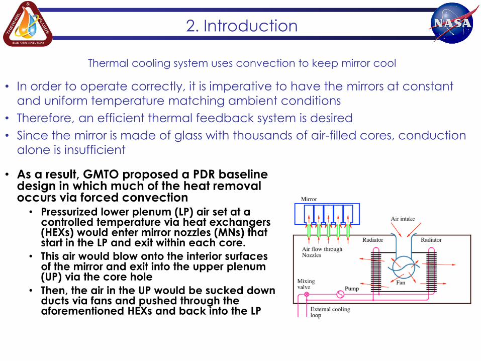
2. Introduction

• In order to operate correctly, it is imperative to have the mirrors at constant

and uniform temperature matching ambient conditions

• Therefore, an efficient thermal feedback system is desired

• Since the mirror is made of glass with thousands of air-filled cores, conduction

alone is insufficient

• As a result, GMTO proposed a PDR baseline design in which much of the heat removal occurs via forced convection

• Pressurized lower plenum (LP) air set at a controlled temperature via heat exchangers (HEXs) would enter mirror nozzles (MNs) that start in the LP and exit within each core.

• This air would blow onto the interior surfaces of the mirror and exit into the upper plenum (UP) via the core hole

• Then, the air in the UP would be sucked down ducts via fans and pushed through the aforementioned HEXs and back into the LP

Overview

3. Methods

The methodology performed followed the flow chart provided

1. First, the flow network was defined

2. CFD parametric breakout models were analyzed

3. MATLAB script using results from #1 & #2 as inputs output heat transfer coefficients (HTCs)

4. Thermal model as analyzed and thermal time constants and temperatures were post-processed

1. Flow Network: understanding pressure and flow rate at all

locations

3. Methods

• Thermal cooling system is a closed loop system consisting of numerous parts (MNs, HEXs, etc)• As a result, there is a need to force the air to circulate (e.g.-fans)

• Fan performance varies with driving pressure• Moreover, the effectiveness of the thermal cooling system is dependent on the

amount of flow being blown out through the nozzles

• Therefore, it was necessary to understand the characteristics of the airflow within the system (e.g.-flow network)

• Flow networks allow the engineer to understand and predict the behavior of the fluid at different “stations”• Thus it allows for the engineer to know the pressure drop across stations and

the resulting fan flow rates

3. Methods

Flow Network: summation of minor losses

Flow Network Schematic of Stations

Fan Pressure Curve Sudden Contraction Minor Loss HEX Pressure Curve

Created CFD breakout models to determine missing minor

losses and unknown HTCs

3. Methods

• It would be too computationally intensive to perform numerous CFD simulations of the entire mirror

• As a result, breakout models of either a single core, or a region of cores were created to determine the effects of the nozzles & flow rates have on the HTCs

• A core close to the center of the mirror and close to the edge (Core 22 & 193, respectively) were selected for the breakout models

• Moreover, Cores 209 & 222 were chosen since they were no perfectly hexagonal

• Each breakout model was parameterized to have variable nozzle length, nozzle diameter, and mass flow rate/inlet pressure

Analyzed three different CFD breakout models

3. Methods

• Three different types of breakout models were created:• “core”

• Used for PDR baseline design (until additional information was needed)

• “core + UP fan”

• Used for PDR baseline design

• “core + UP”

• Used for Optimized UPN design

“core + UP fan”

“core + UP”“core”

Performed CFD parametric study to estimate thermal time

constants

3. Methods

• Ran steady state solutions, and calculated HTCs on the different surfaces

• Moreover, calculated thermal time constants on the 3 different regions of each core• Each region consisted of “major” parts

of the mirror (bottom [flat] section, top [parabolic] section, and side [core walls] section)

• The goal was to find a set of parameters that would result in the same thermal time constant for all cores

Thermal Time Constant Equation

(i = region, n = surface)

Determined Nusselt number correlation

coefficients

3. Methods

• Once HTCs were calculated for these

specific breakout models, Nusselt

Number (Nu) correlations were

developed so that HTCs could be

predicted for all cores/conditions

• For each surface, a known Nu

correlation was compared to the CFD

derived Nu

• The known Nu correlation was “tweaked”

until it matched (see boxes below)

n = 1.1319 X = 0.111 Abot = 0.0228 m2 Aback = 0.265 m2

Developed MATLAB script to calculate HTCs for all surfaces

3. Methods

• Now we have Nu correlations and a Flow Network map that are functions of the CFD breakout parameters

• A MATLAB script is written out that allows the user to specify the following inputs:• Number of MN Types

• How many different MNs can the system have

• Fan ID• What fan will the system use

• Fan Number• How many fans in the system

• The output of the script is HTC values for each surface of every core for these specified inputs• Also outputs Fan and HEX Pressure Curves, expected thermal time

constants, MN diameters, and pressure drop

MATLAB script converged to a final solution via flow

network and thermal time constant iterations

3. Methods

• The script does the following:

• Initially guesses MN diameters and pressure drop between LP and

core exit

• Solves the flow network

• Uses the resulting mass flow rates to solve for the Nu correlations

• Calculates the thermal time constants for the top and bottom

regions of each core

• Compares these values

• If the values are not considered close enough to each other, the

script slightly alters either the MN diameters or pressure drop &

repeats Steps 2-5

• Writes out the HTCs for all surfaces of all cores in a format

compatible with Thermal Desktop (TD)

MATLAB script considered flow blockages

3. Methods

• It is important to note that not all cores have MNs due to

components (kinematic constraints, Fan ducts, etc) in the

way

• Approximately 30% of all cores cannot have MNs

• As such, the MATLAB script assumes that these cores have

HTCs of 0 W/m2K for all surfaces except for the back (since

this has UP air circulating over the entire region)

Thermal FEM taken from structural model

3. Methods

• GMTO provided a structural FEM of both the mirror and the mirror cell

• Edited these models to be TD compatible• Made copies of all the side wall elements such

that there were unique EIDs for each core (sets of elements shared the same nodes and were given ½ the thickness)

• Made unique Property IDs for each core and region of interest (top, bottom, sides)

Received Mirror FEM

Received Mirror Cell FEM

Edited Mirror FEM

Made adjustments to FEM to create thermal model

3. Methods

• Imported edited FEMs into TD

• Additional edits were made to the model• Representing certain components as diffusion nodes

• Adding boundary nodes

• Including conductors/contactors to represent thermal couplings between components that don’t share nodes

• Including natural and forced convection contactors

• Forced convection contactors used symbols to define their HTCs

• Writing “logic blocks” (i.e. – code) which read in the output of the MATLAB scripts to provide values to the HTC symbols

• Including radiation between the top surface of the mirror and the night sky

• Did not include surface to surface radiation since the emissivity of glass is low & the mirror is assumed to be at near uniform temperature

3. Methods

Final thermal model

Thermal load case used to compare designs

3. Methods

• The entire cell is assumed to be a constant initial temperature:

Tinit = 13 °F

• At time t = 0 s, the doors of the chamber are assumed to open,

and outside air (which is at a temperature of Tconv = 11 °F) enters

• For a duration of 10 hours, the thermal cooling system blows Tconv

air onto the mirror to cool it to the same temperature as

ambient

• Calculates the temperature of the mirror as a function of time as

well as the resulting thermal time constants

PDR baseline design used HTC correlations instead of Nu

4. Results

• PDR baseline design assumed all MNs were the same length and diameter

• As a result, Nu correlations described previously were not used

• Used direct HTC correlations shown in the upper figure

• Since cores become taller and taller as you move radially outward (see picture below), this results in the HTCs on the top surfaces varying as a function of radius

• Other HTCs were constant

• The HTCs on the back surface were found to be a function of the velocity of the air leaving the cores as shown in the lower figure

• The MATLAB script previously defined as altered to account for these new HTC correlations

PDR baseline design showed non-uniform temperatures

4. Results

• The MATLAB script wrote out the resulting HTCs for all cores as well as the plots shown below

• These HTCs were included into the thermal model, and the resulting temperature contour is shown to the right

PDR baseline design temperatures vs time showed top and

bottom surfaces at different temperatures

4. Results

PDR baseline design resulted in large and non-uniform

thermal time constants

4. Results

• The resulting thermal time constants (in minutes) are plotted on the figure to the right

• Top Surface• Bottom Surface

• For the top surface: near the center of the mirror, the thermal time constants are smaller (due to the MNs being close to the top surface), but as you go radially outward, the thermal time constants increase

• For the bottom surface: thermal time constants are relatively constant due to good uniform circulation in the UP

• For both surfaces: triangular patterns of large thermal time constants exist due to flow blockages in the UP preventing MNs from entering those cores

Optimization of baseline design could not be achieved

4. Results

• By assuming different MN lengths and diameters throughout the thermal control system, attempted to optimize the Baseline Design

• However, after numerous CFD breakout models, determined that it was difficult, if not impossible, to achieve a constant thermal time constant for all cores on both the top and bottom regions

• Therefore, developed a new design

Nu correlations from optimization attempts

4. Results

Nu correlations were validated during the attempt to optimize the baseline design

Optimized UPN design allows for decoupling of top and

bottom thermal time constants

4. Results

• Developed a design whereby additional nozzles are

included: Upper Plenum Nozzles (UPNs)

• These nozzles go from the LP to the UP (just below the back surface

of the mirror)

• This was found to induce impinging jet flow on the back surface of

the mirror, thus decreasing its thermal time constant

• Meanwhile, MNs can be tailored to impinge on the top surface of

the mirror, thus decreasing its thermal time constants

• By having two sets of nozzles, we make each region’s

thermal time constants independent of each other, and

the nozzles can be tailored for each

Chose a maximum of 2 UPNs per core for Optimized UPN

design

4. Results

• Proposed to have as many as 6 UPNs per core as shown in the figure in the upper right

• However, as previously stated, due to flow blockages/other components, not all cores could have up to 6 UPNs

• The figure on the bottom right shows the back surface of the mirror and the potential UPN locations (in red) as well as the cores that cannot have MNs (in black)

• ATA/GMTO agreed to have a maximum of 2 UPNs per core

• With the flow blockages, this resulted in 62% of the cores having 2 UPNs, 12% having 1, and 26% having none

Optimized UPN design resulted in low and uniform

estimated thermal time constants

4. Results

• With the new design, Nu correlations for the back surface

were update to:

• Was able to pick UPN diameters and lengths to get

matching thermal time constants

Optimized UPN design showed uniform

temperatures

4. Results

Ran MATLAB script by assuming 3

MN types (instead of 1 for PDR

Baseline) and same Fan ID and Fan

#s as PDR Baseline

Optimized UPN design temperatures vs time showed top

and bottom surfaces at same temperatures for “ideal cores”

4. Results

Optimized UPN design resulted in small and uniform thermal

time constants

4. Results

• The resulting thermal time constants (in minutes) are plotted on the figure to the right• Top Surface• Bottom Surface

• For the top surface: thermal time constants are constant throughout

• For the bottom surface: thermal time constants are constant throughout

• For both surfaces: triangular patterns of large thermal time constants exist due to flow blockages in the UP preventing MNs from entering those cores

Comparisons show optimized UPN design outperforms PDR

baseline design dramatically

5. Conclusions

Summary

5. Conclusions

• Analyzed GMTO’s PDR Baseline Design and found similar thermal time constants to what was seen in similar telescopes

• Attempted to optimize the baseline design, but found that a uniform and low thermal time constant could not be achieved

• Developed a new design which met all the goals/objectives of GMTO• New design reduced the thermal time constant by a factor of two

and improved uniform temperature distribution by a factor of 5

• In the process, used CFD (Star-CCM+), MATLAB, Thermal Desktop as well as other software (NX, excel, etc) for the project