
Damiano Pasetto
35
Laboratory of ecohydrology ´ Ecole polytechnique f ´ ed´ erale de Lausanne Data assimilation for distributed models: an overview of applications with CATHY Damiano Pasetto Workshop on coupled hydrological modeling Padova, 24 Sept. 2015 Damiano Pasetto DA for distributed models Padova - 24 September 2015
-
Upload
coupledhydrologicalmodeling -
Category
Science
-
view
291 -
download
0
Transcript of Damiano Pasetto

Laboratory of ecohydrologyEcole polytechnique federalede Lausanne
Data assimilation for distributed models:an overview of applications with CATHY
Damiano Pasetto
Workshop on coupled hydrological modelingPadova, 24 Sept. 2015
Damiano Pasetto DA for distributed models Padova - 24 September 2015

Table of Contents
Table of Contents
1 Introduction
2 Data assimilation methods
3 Hydrological applications
Damiano Pasetto DA for distributed models Padova - 24 September 2015

Introduction Motivations
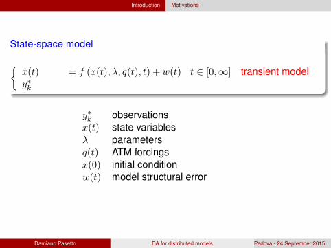
State-space model
{x(t) = f (x(t), λ, q(t), t) + w(t) t ∈ [0,∞] transient modely∗k
↔ yk = h (x, tk) + vk k = 1, . . . observation model
y∗k observationsx(t) state variables
p (x(t))λ parameters p(λ)q(t) ATM forcingsx(0) initial conditionw(t) model structural errorvk measurement error
Damiano Pasetto DA for distributed models Padova - 24 September 2015
Introduction Motivations
State-space model
{x(t) = f (x(t), λ, q(t), t) + w(t) t ∈ [0,∞] transient modely∗k
↔ yk = h (x, tk) + vk k = 1, . . . observation model
y∗k observationsx(t) state variables
p (x(t))
λ parameters
p(λ)
q(t) ATM forcingsx(0) initial conditionw(t) model structural error
vk measurement error
Damiano Pasetto DA for distributed models Padova - 24 September 2015

Introduction Motivations
State-space model
{x(t) = f (x(t), λ, q(t), t) + w(t) t ∈ [0,∞] transient modely∗k ↔ yk = h (x, tk) + vk k = 1, . . . observation model
y∗k observationsx(t) state variables
p (x(t))
λ parameters
p(λ)
q(t) ATM forcingsx(0) initial conditionw(t) model structural errorvk measurement error
Damiano Pasetto DA for distributed models Padova - 24 September 2015

Introduction Motivations
State-space model
{x(t) = f (x(t), λ, q(t), t) + w(t) t ∈ [0,∞] transient modely∗k ↔ yk = h (x, tk) + vk k = 1, . . . observation model
y∗k observationsx(t) state variables p (x(t))λ parameters
p(λ)
q(t) ATM forcingsx(0) initial conditionw(t) model structural errorvk measurement error
Damiano Pasetto DA for distributed models Padova - 24 September 2015

Introduction Motivations
State-space model
{x(t) = f (x(t), λ, q(t), t) + w(t) t ∈ [0,∞] transient modely∗k ↔ yk = h (x, tk) + vk k = 1, . . . observation model
y∗k observationsx(t) state variables p (x(t))λ parameters p(λ)q(t) ATM forcingsx(0) initial conditionw(t) model structural errorvk measurement error
Damiano Pasetto DA for distributed models Padova - 24 September 2015

Introduction Motivations
MotivationsHydrological forecasting is subject to many sources of uncertainty
Initial conditionForcing termsModel parameters(Model itself?)
Data Assimilation (DA)Correct the model forecast considering the measurements
State . . . xk−1 → x−k xk → x−k+1 . . .↓ ↑ ↓
Observations . . . y−k ↔ y∗k . . .
Forecast pdf: π−(x(tk) | y1, . . . , yk−1)Filtering pdf: π+(x(tk) | y1, . . . , yk−1, yk)
Damiano Pasetto DA for distributed models Padova - 24 September 2015

Introduction Motivations
MotivationsHydrological forecasting is subject to many sources of uncertainty
Initial conditionForcing termsModel parameters(Model itself?)
Data Assimilation (DA)Correct the model forecast considering the measurements
State . . . xk−1 → x−k xk → x−k+1 . . .↓ ↑ ↓
Observations . . . y−k ↔ y∗k . . .
Forecast pdf: π−(x(tk) | y1, . . . , yk−1)
Filtering pdf: π+(x(tk) | y1, . . . , yk−1, yk)
Damiano Pasetto DA for distributed models Padova - 24 September 2015

Introduction Motivations
MotivationsHydrological forecasting is subject to many sources of uncertainty
Initial conditionForcing termsModel parameters(Model itself?)
Data Assimilation (DA)Correct the model forecast considering the measurements
State . . . xk−1 → x−k xk → x−k+1 . . .↓ ↑ ↓
Observations . . . y−k ↔ y∗k . . .
Forecast pdf: π−(x(tk) | y1, . . . , yk−1)Filtering pdf: π+(x(tk) | y1, . . . , yk−1, yk)
Damiano Pasetto DA for distributed models Padova - 24 September 2015

Introduction A simple example with CATHY
Example: application to CATHY (CATchment HYdrology)
Coupled surface/subsurface modelRichards equation:
Sw(ψ)Ss∂ψ
∂t+ φ
∂Sw(ψ)
∂t= ∇ · [KsKrw(Sw(ψ)) (∇ψ + ηz)] + qss(h)
1-D path-based surface routing:
∂Q
∂t+ ck
∂Q
∂s= Dh
∂2Q
∂s2+ ckqs(h, ψ)
BC-switching/forcing algorithm
State variables: x = {ψ,Q}.Measures: piezometric head, soil moisture, streamflow, electricpotential (ERT).
(Camporese et al. 2010, WRR)Damiano Pasetto DA for distributed models Padova - 24 September 2015

Introduction A simple example with CATHY
DA: example on the V-catchment
3 m soil depthAssimilation of streamflow
Uncertainty:Initial conditionsATM forcings
Damiano Pasetto DA for distributed models Padova - 24 September 2015

Introduction A simple example with CATHY
Forecast considering model uncertainties (open loop)
0 1800 3600 5400 7200 9000 10800 12600 144000
1
2
3
4
5
6St
ream
flow
(m
3 /s) TRUE
ObservationsOpen Loop
0 1800 3600 5400 7200 9000 10800 12600 14400Time (s)
1.939
1.940
1.941
1.942
1.943
1.944
Wat
er S
tora
ge (
106 m
3 )
Damiano Pasetto DA for distributed models Padova - 24 September 2015

Introduction A simple example with CATHY
Assimilation of measurement of streamflow
0 1800 3600 5400 7200 9000 10800 12600 144000
1
2
3
4
5
6St
ream
flow
(m
3 /s) TRUE
ObservationsSIR
0 1800 3600 5400 7200 9000 10800 12600 14400Time (s)
1.939
1.940
1.941
1.942
1.943
1.944
Wat
er S
tora
ge (
106 m
3 )
Damiano Pasetto DA for distributed models Padova - 24 September 2015

Data assimilation methods EnKF and SIR
Forecast step: MC simulation
xi0 ∼ p(x0), i = 1, . . . , N Initial samples
xi,−k = f(xik−1, λi, qik, tk) + wi
k Forecast
Analysis stepEnsemble Kalman filter (EnKF, Evensen 1994): Kalman gain
xik = xi,−k +Kk
(y∗k − h(x
i,−k )
)
Sequential Importance Resampling (SIR):weighted realizations
(xik, ω
ik
)update weights with the likelihood and normalize
ωik = Cωi
k−1L(y∗k |xi,−k )
duplicate particles that have largest weights.
Damiano Pasetto DA for distributed models Padova - 24 September 2015

Data assimilation methods EnKF and SIR
Forecast step: MC simulation
xi0 ∼ p(x0), i = 1, . . . , N Initial samples
xi,−k = f(xik−1, λi, qik, tk) + wi
k Forecast
Analysis stepEnsemble Kalman filter (EnKF, Evensen 1994): Kalman gain
xik = xi,−k +Kk
(y∗k − h(x
i,−k )
)Sequential Importance Resampling (SIR):
weighted realizations(xik, ω
ik
)update weights with the likelihood and normalize
ωik = Cωi
k−1L(y∗k |xi,−k )
duplicate particles that have largest weights.
Damiano Pasetto DA for distributed models Padova - 24 September 2015

Data assimilation methods EnKF and SIR
Damiano Pasetto DA for distributed models Padova - 24 September 2015

Hydrological applications 1. Geophysical coupled inversion
1. Geophysical coupled inversion: Electrical Resistivity Tomography
(Rossi et al. 2015, AWR)Damiano Pasetto DA for distributed models Padova - 24 September 2015

Hydrological applications 1. Geophysical coupled inversion
Iterative particle filter
(Manoli et al. 2015, JCP)Damiano Pasetto DA for distributed models Padova - 24 September 2015

Hydrological applications 1. Geophysical coupled inversion
Damiano Pasetto DA for distributed models Padova - 24 September 2015

Hydrological applications 2. Landscape Evolution Observatory (LEO)
2. Landscape Evolution Observatory (LEO)
Three convergent landscapes
30 m long, 11 m wide, 1 m soil
10 degrees average slope
Environmentally controlledgreenhouse facility
Landscape instrumentation
rainfall simulator(3-45 mm/h)
10 load cells
6 flow meters forseepage faceoutflow
1,835 sensorsembedded in thesoil
Damiano Pasetto DA for distributed models Padova - 24 September 2015

Hydrological applications 2. Landscape Evolution Observatory (LEO)
First experiment at LEO (18 February 2013)
Experiment setup:
Unsaturated initialconditions
Imposed rainfall:≈12 mm/h
With homogeneous soil,steady state expectedafter 36 h
After the experiment: the rainfall wasstopped after 22 h due to the occurrenceof overland flow.
Damiano Pasetto DA for distributed models Padova - 24 September 2015

Hydrological applications 2. Landscape Evolution Observatory (LEO)
Synthetic scenario reproducing Experiment 1 at LEO
Assumption: Y = log(KS) is a Gaussian random field with exponentialcovariance function. E[KS ] = 10−4 m/s with coefficient of variation100% (µY = −9.56, σY = 0.83)
Test case 1 (TC1): λx = λy = 8 m; λz= 0.5 mTest case 2 (TC2): λx = λy = 4 m; λz= 0.25 m
Number of grid cells: 60×22×20= 26400
Sensor failure analysisThe assimilation is repeated decreasing the number of measurements,from m=496 to m= 21 active sensors.
(Pasetto et al. 2015, AWR)
Damiano Pasetto DA for distributed models Padova - 24 September 2015

Hydrological applications 2. Landscape Evolution Observatory (LEO)
−5 0 5
5
10
15
20
25
d= 0.00÷0.05 m
x (m)
y (m
)
−5 0 5
5
10
15
20
25
d= 0.15÷0.20 m
x (m)−5 0 5
5
10
15
20
25
d= 0.30÷0.35 m
x (m)−5 0 5
5
10
15
20
25
d= 0.50÷0.55 m
x (m)−5 0 5
5
10
15
20
25
d= 0.80÷0.85 m
x (m)−5 0 5
5
10
15
20
25
d= 0.95÷1.00 m
x (m)
10−5
10−4
10−3
K S (m
/s)
True
−5 −2 0 2 5
5
10
15
20
25
d= 0.00÷0.05 m
x (m)
y (m
)
−5 −2 0 2 5
5
10
15
20
25
d= 0.15÷0.20 m
x (m)−5 −2 0 2 5
5
10
15
20
25
d= 0.30÷0.35 m
x (m)−5 −2 0 2 5
5
10
15
20
25
d= 0.50÷0.55 m
x (m)−5 −2 0 2 5
5
10
15
20
25
d= 0.80÷0.85 m
x (m)−5 −2 0 2 5
5
10
15
20
25
d= 0.95÷1.00 m
x (m)
10−5
10−4
10−3
K S (m
/s)
m= 496
True and estimated spatial distributions of KS in TC2.Damiano Pasetto DA for distributed models Padova - 24 September 2015
Hydrological applications 2. Landscape Evolution Observatory (LEO)
0
0.5
1
1.5
Ove
rland
Flo
w (m
3 /h)
EnsembleEnsemble MeanTrue90% C.I.
TC1 (long correlation length)
0
0.5
1
1.5
Seep
age
Face
Flo
w (m
3 /h)
0 4 8 12 16 20 24 28 32 36Time t (h)
40
60
80
100
120
Wat
er S
tora
ge (m
3 )
TC2 (short correlation length)
0 4 8 12 16 20 24 28 32 36Time t (h)
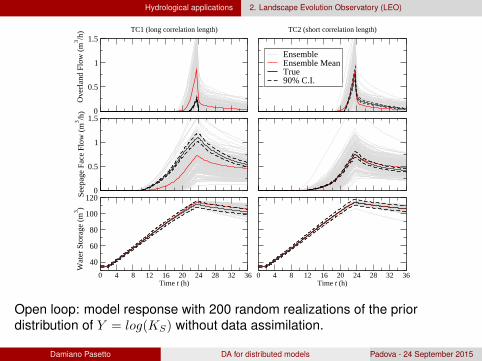
Open loop: model response with 200 random realizations of the priordistribution of Y = log(KS) without data assimilation.
Damiano Pasetto DA for distributed models Padova - 24 September 2015

Hydrological applications 2. Landscape Evolution Observatory (LEO)
0
0.5O
verla
nd (m
3 /h)
Truem= 496m= 196m= 46m= 21
TC1 (long correlation length)
0
0.5
1
1.5
Seep
age
(m3 /h
)
406080
100120
Stor
age
(m3 )
0 4 8 12 16 20 24 28Time t (h)
0.001
0.01
RM
SE o
n vw
c
TC2 (short correlation length)
0 4 8 12 16 20 24 28 32 36Time t (h)
Model response with the calibrated saturated hydraulic conductivity
Damiano Pasetto DA for distributed models Padova - 24 September 2015

Conclusions
Conclusions
Data assimilation methods help improve the forecast and reduce theuncertainty of high dimensional hydrological models.
Data assimilation methods allow the online estimation of both the statevariables and the model parameters.
Work in progress
Covariance localization and ensemble inflation to minimizeill-conditioning and filter inbreeding in the EnKF update.Update step performed with a combination of EnKF and SIR(Gaussian Mixture Filters)Surrogate models to accelerate the Monte Carlo simulation.
Damiano Pasetto DA for distributed models Padova - 24 September 2015

Conclusions
Thank you for your attention
ReferencesD Pasetto, M Camporese, and M Putti. Ensemble Kalman filter versus particle filter for aphysically-based coupled surface-subsurface model, Adv Water Resources, 2012.G Manoli, M Rossi, D Pasetto, R Deiana, S Ferraris, G Cassiani, and M Putti. An iterativeparticle filter approach for coupled hydro-geophysical inversion of a controlled infiltrationexperiment, J Comp Phys, 2015.M Rossi, G Manoli, D Pasetto, R Deiana, S Ferraris, C Strobbia, M Putti, G Cassiani.Coupled inverse modeling of a controlled irrigation experiment using multiplehydro-geophysical data, Adv Water Resources, 2015.D Pasetto, G-Y Niu, L Pangle, C Paniconi, M Putti, PA Troch. Impact of sensor failure onthe observability of flow dynamics at the Biosphere 2 LEO hillslopes, Adv WaterResources, 2015.
Damiano Pasetto DA for distributed models Padova - 24 September 2015

Conclusions
Damiano Pasetto DA for distributed models Padova - 24 September 2015

Conclusions
Damiano Pasetto DA for distributed models Padova - 24 September 2015

Conclusions
Damiano Pasetto DA for distributed models Padova - 24 September 2015

Conclusions
Damiano Pasetto DA for distributed models Padova - 24 September 2015