Damage Detection in Civil Structures Using

High-Frequency Seismograms

Thesis by

Vanessa Heckman

In Partial Fulfillment of the Requirements

for the Degree of

Doctor of Philosophy

California Institute of Technology

Pasadena, California

2014

(Defended September 27, 2013)

© 2014

Vanessa Heckman

All Rights Reserved

ii

To my parents and brother.

iii

Acknowledgements

I would like to thank my adviser, Tom Heaton, for sharing his enthusiasm and wisdom with

me throughout the years. I will always happily remember discussing research results with

him in his office, and I am very appreciative of his willingness to meet with me to discuss

research for hours at a time and for keeping his door always open.

To Monica Kohler for, in many ways, serving as a second adviser to me. She’s been a great

role model throughout the years, and I’ve learned a lot from her professionally, especially as

an experimentalist and a technical writer.

To Rob Clayton for welcoming me to his group meetings and serving as a geophysics

mentor to me in my earlier years of graduate school when I went to my first conference,

undoubtedly the largest conference I will ever attend (the AGU). Thanks also for his patience.

To Jim Beck, for discussions related to math and history of science. Also for his guidance

in research topics in damage detection and in daring to teach mathematics to engineers.

To Victor Tsai for his feedback during my thesis talk.

To Masumi Yamada, for welcoming me to Uji Campus, Kyoto University for my EAPSI

project and making my summer research experience a special one. I will always look up to

Masumi as an amazing researcher and speaker.

To John Hall, my adviser during college, for taking the time to cultivate my passion for

civil engineering.

To Ken Pickar, for welcoming our group of CE students into his entrepreneurship class

and taking the time to meet with us to provide an honest, well-informed opinion on our

project.

To Swami Krishnan, for his involvement in public outreach programs with me.

iv

To Joann Stock for welcoming me on the seismic field trips, especially to the Salton Sea

(where I got to create my first ‘earthquake’ from a borehole explosion).

To Luke Wang and Bill Iwan for their mentorship.

To Kaushik Bhattacharya for meeting with me during college to discuss Timoshenko.

To Brad Aagaard for developing his amazing code PyLith and for helping to get it up

and running on the GPS and CE computing clusters. I am confident that his endeavors in

creating this program will reward many researchers to come.

To Case Bradford for taking the time to work with me on the Millikan library project

when I was still an undergraduate.

To Carolina Oseguera and Chris Silva, who kept Thomas running and yet still found the

time to be supportive of the students.

To Raul for fixing the equipment for class and for telling me stories about the old CE

department as he was doing so.

Also a special thanks to all of the friends I made through my involvement with the EERI

student leadership council. Nima, Erica, David, Tim, Maria, Karthik, Evgueni, Jeff, Manny,

Jasmine, Charlie, Michael, Andreas, we did it! To the UC Memphis faculty for letting us

borrow their shake table. To the staff at EERI and President-Elect Tom Tobin, it was a

pleasure working with you. To Ashraf at CSI for daring to dream big and inspiring others

to do so. To the friends I made through my involvement in APSS and EAPSI, especially

Christiana, Emily, Austin, and Ben.

A special thanks to my friends in the CE and GPS departments, who have been my coffee

buddies throughout the years: Matt, Dan, Anna, Ahmed, In Ho, Trevor, Ramses, Stephen,

Michael, Song, Hemanth, Mohsen, Navneet, Surendra, Nathalie, Grant, Arnar, Swetha, Dan,

Dani, June. To the Painter group and Tirrell lab members: Ari, Amir, Jasper, Jeffs. J.D.,

Rob, Dvin. To my art class friends Christine and Patrick. Tiffany, Tim, Iram, Juhwan,

Alice, Lydia, and Sangita. To Cedric and Ming, who encouraged me to reattend Caltech for

graduate school. To my high school friends Omid, Zach, Logan, and Natasha.

Finally, thank you to my family for their love and support: my parents, Nate, Brett and

the kitties.

v

Abstract

The dynamic properties of a structure are a function of its physical properties, and changes

in the physical properties of the structure, including the introduction of structural damage,

can cause changes in its dynamic behavior. Structural health monitoring (SHM) and damage

detection methods provide a means to assess the structural integrity and safety of a civil

structure using measurements of its dynamic properties. In particular, these techniques

enable a quick damage assessment following a seismic event. In this thesis, the application

of high-frequency seismograms to damage detection in civil structures is investigated.

Two novel methods for SHM are developed and validated using small-scale experimental

testing, existing structures in situ, and numerical testing. The first method is developed for

pre-Northridge steel-moment-resisting frame buildings that are susceptible to weld fracture

at beam-column connections. The method is based on using the response of a structure to a

nondestructive force (i.e., a hammer blow) to approximate the response of the structure to

a damage event (i.e., weld fracture). The method is applied to a small-scale experimental

frame, where the impulse response functions of the frame are generated during an impact

hammer test. The method is also applied to a numerical model of a steel frame, in which weld

fracture is modeled as the tensile opening of a Mode I crack. Impulse response functions

are experimentally obtained for a steel moment-resisting frame building in situ. Results

indicate that while acceleration and velocity records generated by a damage event are best

approximated by the acceleration and velocity records generated by a colocated hammer

blow, the method may not be robust to noise. The method seems to be better suited for

damage localization, where information such as arrival times and peak accelerations can also

provide indication of the damage location. This is of significance for sparsely-instrumented

vi

civil structures.

The second SHM method is designed to extract features from high-frequency accelera-

tion records that may indicate the presence of damage. As short-duration high-frequency

signals (i.e., pulses) can be indicative of damage, this method relies on the identification and

classification of pulses in the acceleration records. It is recommended that, in practice, the

method be combined with a vibration-based method that can be used to estimate the loss of

stiffness. Briefly, pulses observed in the acceleration time series when the structure is known

to be in an undamaged state are compared with pulses observed when the structure is in

a potentially damaged state. By comparing the pulse signatures from these two situations,

changes in the high-frequency dynamic behavior of the structure can be identified, and dam-

age signals can be extracted and subjected to further analysis. The method is successfully

applied to a small-scale experimental shear beam that is dynamically excited at its base

using a shake table and damaged by loosening a screw to create a moving part. Although

the damage is aperiodic and nonlinear in nature, the damage signals are accurately identi-

fied, and the location of damage is determined using the amplitudes and arrival times of the

damage signal. The method is also successfully applied to detect the occurrence of damage

in a test bed data set provided by the Los Alamos National Laboratory, in which nonlinear

damage is introduced into a small-scale steel frame by installing a bumper mechanism that

inhibits the amount of motion between two floors. The method is successfully applied and

is robust despite a low sampling rate, though false negatives (undetected damage signals)

begin to occur at high levels of damage when the frequency of damage events increases. The

method is also applied to acceleration data recorded on a damaged cable-stayed bridge in

China, provided by the Center of Structural Monitoring and Control at the Harbin Institute

of Technology. Acceleration records recorded after the date of damage show a clear increase

in high-frequency short-duration pulses compared to those previously recorded. One un-

damage pulse and two damage pulses are identified from the data. The occurrence of the

detected damage pulses is consistent with a progression of damage and matches the known

chronology of damage.

vii

Contents

Acknowledgements iv

Abstract vi

1 Introduction 1

1.1 Structural Damage . . . . . . . . . . . . . . . . . . . . . . . . . . . . . . . . 8

1.1.1 Structural Damage to Buildings in the United States . . . . . . . . . 10

1.1.2 1994 Northridge Earthquake: Lessons Learned . . . . . . . . . . . . . 11

1.1.3 Using High-Frequency Seismograms for Damage Detection . . . . . . 16

1.2 Structural Health Monitoring and

Damage Detection Methods . . . . . . . . . . . . . . . . . . . . . . . . . . . 18

1.2.1 Vibration-Based Techniques . . . . . . . . . . . . . . . . . . . . . . . 19

1.2.1.1 Natural Frequency Based Methods . . . . . . . . . . . . . . 20

1.2.1.2 Mode Shape Based Methods . . . . . . . . . . . . . . . . . . 20

1.2.1.3 Flexibility/Stiffness Based Methods . . . . . . . . . . . . . . 22

1.2.1.4 Parameter Estimating and Updating . . . . . . . . . . . . . 23

1.2.2 Acoustic Methods . . . . . . . . . . . . . . . . . . . . . . . . . . . . . 24

1.2.2.1 Guided-Wave Methods . . . . . . . . . . . . . . . . . . . . . 24

1.2.3 Time-Frequency Signal Analysis . . . . . . . . . . . . . . . . . . . . . 26

1.2.3.1 Analytic Signal . . . . . . . . . . . . . . . . . . . . . . . . . 26

1.2.3.2 Time-Frequency Distributions . . . . . . . . . . . . . . . . . 27

1.2.4 Other Methods . . . . . . . . . . . . . . . . . . . . . . . . . . . . . . 28

viii

1.2.5 Validation and Comparative Studies . . . . . . . . . . . . . . . . . . 29

1.2.5.1 Publicly-Available Datasets for the Purpose of Benchmarking 29

1.2.5.2 Datasets Used in this Thesis for the Purpose of Validation . 38

2 Experimental Study:

Damage Detection Method for

Weld Fracture of Beam-Column Connections in Steel Moment-Resisting-

Frame Buildings 39

2.1 Introduction . . . . . . . . . . . . . . . . . . . . . . . . . . . . . . . . . . . . 40

2.2 Description of Proposed Damage Detection Method . . . . . . . . . . . . . . 41

2.3 Experimental Study: Small-Scale Steel Frame . . . . . . . . . . . . . . . . . 43

2.3.1 Experimental Setup . . . . . . . . . . . . . . . . . . . . . . . . . . . . 43

2.3.2 Experimental Results and Discussion . . . . . . . . . . . . . . . . . . 45

2.3.3 Blind Tap Test . . . . . . . . . . . . . . . . . . . . . . . . . . . . . . 51

2.4 Experimental Study:

Steel Moment-Resisting Frame Building . . . . . . . . . . . . . . . . . . . . . 54

2.5 Conclusion . . . . . . . . . . . . . . . . . . . . . . . . . . . . . . . . . . . . . 55

3 Experimental Shear Beam 68

3.1 Experimental Setup and Method . . . . . . . . . . . . . . . . . . . . . . . . 69

3.2 Theoretical Model:

Linear Multi-Degree of Freedom System . . . . . . . . . . . . . . . . . . . . 72

3.2.1 Undamaged Frame . . . . . . . . . . . . . . . . . . . . . . . . . . . . 74

3.2.2 Damaged Frame . . . . . . . . . . . . . . . . . . . . . . . . . . . . . . 77

3.2.2.1 Damage Model I . . . . . . . . . . . . . . . . . . . . . . . . 78

3.2.2.2 Damage Model II . . . . . . . . . . . . . . . . . . . . . . . . 80

3.3 Experimental Results . . . . . . . . . . . . . . . . . . . . . . . . . . . . . . . 81

3.3.1 Linearity of the Damaged and Undamaged Shear Beam . . . . . . . . 82

ix

3.3.2 Static Testing:

Stiffness Parameter Estimation via a Tilt Test . . . . . . . . . . . . . 84

3.3.3 Dynamic Testing: Damage Levels 1, 2, and 3 . . . . . . . . . . . . . . 90

3.3.4 Dynamic Testing:

Damage Detection Method Based on Pulse Identification . . . . . . . 96

3.3.5 Comparison of Experimental and Theoretical Models: Undamaged

Frame . . . . . . . . . . . . . . . . . . . . . . . . . . . . . . . . . . . 101

3.4 Conclusion . . . . . . . . . . . . . . . . . . . . . . . . . . . . . . . . . . . . . 105

4 Numerical Study:

Time-Reversed Reciprocal Method and Damage Detection Method for

Weld Fracture 114

4.1 Comparison of Structural Response to Two Different Source Conditions . . . 115

4.1.1 Stacked Cross-Correlation Values . . . . . . . . . . . . . . . . . . . . 117

4.2 A Time-Reversed Reciprocal Method . . . . . . . . . . . . . . . . . . . . . . 119

4.2.1 Forward Simulation . . . . . . . . . . . . . . . . . . . . . . . . . . . . 120

4.2.2 Reverse Simulation . . . . . . . . . . . . . . . . . . . . . . . . . . . . 123

4.3 Conclusions . . . . . . . . . . . . . . . . . . . . . . . . . . . . . . . . . . . . 123

5 Application of High-Frequency Damage Detection Methods to Benchmark

Problems 126

5.1 Nonlinear Frame . . . . . . . . . . . . . . . . . . . . . . . . . . . . . . . . . 126

5.1.1 Identification of Damage Signals Through Feature Extraction of Pulses 131

5.2 Damaged Cable-Stayed Bridge in China . . . . . . . . . . . . . . . . . . . . 134

5.2.1 Identification of Damage Signals Through Feature Extraction of Pulses 138

5.3 Conclusion . . . . . . . . . . . . . . . . . . . . . . . . . . . . . . . . . . . . . 140

6 Discussion and Conclusion 148

A Appendix 158

x

A.1 Notation, Definitions, and Properties . . . . . . . . . . . . . . . . . . . . . . 158

A.2 Publications . . . . . . . . . . . . . . . . . . . . . . . . . . . . . . . . . . . . 160

A.3 Uniform Shear Beam . . . . . . . . . . . . . . . . . . . . . . . . . . . . . . . 165

A.4 Application of State Space Method to Acceleration of a High-Rise Building

in Osaka . . . . . . . . . . . . . . . . . . . . . . . . . . . . . . . . . . . . . . 170

A.4.1 Experimental Setup . . . . . . . . . . . . . . . . . . . . . . . . . . . . 171

A.5 State Space Formulation . . . . . . . . . . . . . . . . . . . . . . . . . . . . . 173

A.5.0.1 Differential Equations of Motion . . . . . . . . . . . . . . . 173

A.5.0.2 Canonical Equations . . . . . . . . . . . . . . . . . . . . . . 176

A.5.0.3 State Space Solution . . . . . . . . . . . . . . . . . . . . . . 184

A.5.1 Modal Analysis Using the Laplace Transform Method . . . . . . . . . 188

A.5.2 Transfer Functions, Cross-Correlation, Convolution, and Deconvolution 191

A.5.2.1 Transfer Functions . . . . . . . . . . . . . . . . . . . . . . . 191

A.5.2.2 Cross-Correlation . . . . . . . . . . . . . . . . . . . . . . . . 192

A.5.2.3 Deconvolution . . . . . . . . . . . . . . . . . . . . . . . . . . 194

A.5.2.4 Cross-Correlation with Deconvolution . . . . . . . . . . . . 195

A.5.2.5 Experimental Results . . . . . . . . . . . . . . . . . . . . . 198

A.5.3 Numerical Results:

Damaged vs. Undamaged Building . . . . . . . . . . . . . . . . . . . 199

A.6 Equipment List . . . . . . . . . . . . . . . . . . . . . . . . . . . . . . . . . . 201

Bibliography 206

xi

List of Figures

1.1 1906 San Francisco Earthquake and Fire. . . . . . . . . . . . . . . . . . . . . . 3

1.2 2008 U.S. Geological Survey National Seismic Hazard Map: 1.0-Second Spectral

Acceleration with 10% Probability of Occurrence in 50 Year PE, BC rock. . . 5

1.3 1933 Long Beach Earthquake: Collapse of Unreinforced Masonry Buildings . . 7

1.4 Typical Failure Modes for Welded-Flange-Bolted-Web Connections . . . . . . 14

2.1 Steel Frame: Experimental Setup. . . . . . . . . . . . . . . . . . . . . . . . . . 42

2.2 Steel Frame: Receiver Locations. . . . . . . . . . . . . . . . . . . . . . . . . . 43

2.3 Steel Frame: Example Accelerations. . . . . . . . . . . . . . . . . . . . . . . . 44

2.4 Steel Frame: Comparison of Peak Accelerations in Response to Bolt Fracture

and IRFs. . . . . . . . . . . . . . . . . . . . . . . . . . . . . . . . . . . . . . . 46

2.5 Steel Frame: Example Cross-Correlations. . . . . . . . . . . . . . . . . . . . . 47

2.6 Steel Frame: Comparison of IRFs Before and After Damage. . . . . . . . . . . 50

2.7 Steel Frame: Comparison of Correlation Values Before, During, and After Dam-

age. . . . . . . . . . . . . . . . . . . . . . . . . . . . . . . . . . . . . . . . . . 52

2.8 Steel Frame: Blind Tap Test Using Hammer Blows. . . . . . . . . . . . . . . . 53

2.9 Factor Building: Instrumentation. . . . . . . . . . . . . . . . . . . . . . . . . 54

2.10 Factor Building: Example IRF . . . . . . . . . . . . . . . . . . . . . . . . . . 56

2.11 Factor Building: Comparison of impulse response functions. . . . . . . . . . . 57

3.1 Uniform Shear Beam Experimental Setup. . . . . . . . . . . . . . . . . . . . . 70

3.2 Uniform Shear Beam Models . . . . . . . . . . . . . . . . . . . . . . . . . . . 71

3.3 Consistency Between Trials . . . . . . . . . . . . . . . . . . . . . . . . . . . . 73

xii

3.4 Verification of System Linearity . . . . . . . . . . . . . . . . . . . . . . . . . . 83

3.5 Static Testing: Tilt Table and Schematic . . . . . . . . . . . . . . . . . . . . . 85

3.6 Tilt Test: Damaged vs. Undamaged (Example). . . . . . . . . . . . . . . . . . 86

3.7 Tilt Test: Damaged vs. Undamaged (All Cases). . . . . . . . . . . . . . . . . 88

3.8 Dynamic Testing: Explanatory Schematic. . . . . . . . . . . . . . . . . . . . . 91

3.9 Raw Acceleration Records: Damaged vs. Undamaged. . . . . . . . . . . . . . 92

3.10 Arrival Time Delays: Damaged Frame. . . . . . . . . . . . . . . . . . . . . . . 94

3.11 Shear Beam: Damage Detection Method Using the Detection of Repeating Pulses. 97

3.12 Shear Beam: Raw and High-Frequency Accelerations. . . . . . . . . . . . . . . 98

3.13 Acceleration Pulses: Undamage Signals. . . . . . . . . . . . . . . . . . . . . . 100

3.14 Acceleration Pulses: Damage Signals (Damage State A). . . . . . . . . . . . . 102

3.15 Acceleration Pulses: Damage Signals (Damage State B). . . . . . . . . . . . . 103

3.16 Shear Beam: Analytical vs. Experimental Modeshapes. . . . . . . . . . . . . . 105

3.17 Amplitude of Initial Shear Wave Pulse. . . . . . . . . . . . . . . . . . . . . . . 109

3.18 Experimental Shear Beam: Frequency Response Function. . . . . . . . . . . . 110

3.19 Experimental Shear Beam: Modeshapes (Damaged and Undamaged). . . . . . 111

3.20 Low-Frequency Component of Accelerations. . . . . . . . . . . . . . . . . . . 112

3.21 High-Frequency Component of Accelerations. . . . . . . . . . . . . . . . . . . 113

4.1 Numerical Setup . . . . . . . . . . . . . . . . . . . . . . . . . . . . . . . . . . 116

4.2 High-Frequency Seismograms . . . . . . . . . . . . . . . . . . . . . . . . . . . 118

4.3 Numerical Setup for Steel Frame . . . . . . . . . . . . . . . . . . . . . . . . . 120

4.4 Forward Simulation: Response of Steel Frame to Hammer Blow. . . . . . . . . 121

4.5 Receivers, Sources, and Displacements . . . . . . . . . . . . . . . . . . . . . . 122

4.6 Reverse Simulation: Response of Steel Frame to Prescribed Time-Reversed

Displacements. . . . . . . . . . . . . . . . . . . . . . . . . . . . . . . . . . . . 124

5.1 LANL Nonlinear Frame: Experimental Setup. . . . . . . . . . . . . . . . . . 127

5.2 LANL Nonlinear Frame: Recorded Accelerations (Raw and High-Pass Filtered). 129

5.3 LANL Nonlinear Frame: Amplitude Spectral Density. . . . . . . . . . . . . . 130

xiii

5.4 LANL Nonlinear Frame: Spectrograms for Different Damage Levels at Floor 3. 133

5.5 LANL Nonlinear Frame: Spectrograms for Different Floors at Damage Level 2. 133

5.6 LANL Nonlinear Frame: Damage Signals. . . . . . . . . . . . . . . . . . . . . 135

5.7 LANL Nonlinear Frame: Damage Detection. . . . . . . . . . . . . . . . . . . . 136

5.8 Cable-Stayed Bridge: Dimensions and Instrument Layout. . . . . . . . . . . . 137

5.9 Cable-Stayed Bridge: Sample Deck Accelerations. . . . . . . . . . . . . . . . . 137

5.10 Cable-Stayed Bridge: Undamage and Damage Signals. . . . . . . . . . . . . . 140

5.11 Cable-Stayed Bridge: January 1 Acceleration Records. . . . . . . . . . . . . . 141

5.12 Cable-Stayed Bridge: March 19 Acceleration Records. . . . . . . . . . . . . . 142

5.13 Cable-Stayed Bridge: May 18 Acceleration Records. . . . . . . . . . . . . . . . 143

5.14 Cable-Stayed Bridge: July 31 Acceleration Records. . . . . . . . . . . . . . . . 144

A.1 Simple Shear Beam Synthetics. . . . . . . . . . . . . . . . . . . . . . . . . . . 166

A.2 Wave Propagation in a Shear Beam: Transmission and Reflection Coefficients

for a Variety of Boundary Conditions. . . . . . . . . . . . . . . . . . . . . . . 168

A.3 Wave Propagation in an Infinite Shear Beam with a Low-Velocity Layer. . . . 168

A.4 Osaka High-Rise: Photo of the Building. . . . . . . . . . . . . . . . . . . . . . 172

A.5 Osaka High-Rise: Building Schematic and Model . . . . . . . . . . . . . . . . 174

A.6 Mass-Spring System with Rayleigh Damping . . . . . . . . . . . . . . . . . . . 176

A.7 Numerical Impulse Response Functions . . . . . . . . . . . . . . . . . . . . . . 186

A.8 Numerical Frequency Response Function . . . . . . . . . . . . . . . . . . . . . 187

A.9 Experimental Impulse Response Functions . . . . . . . . . . . . . . . . . . . . 197

A.10 Numerically Computed IRFs. . . . . . . . . . . . . . . . . . . . . . . . . . . . 199

xiv

List of Tables

2.1 Steel Frame: Correlation Values (Undamaged Frame IRFs). . . . . . . . . . . 61

2.2 Steel Frame: Time Errors in Correlations (Undamaged Frame IRFs). . . . . . 62

2.3 Steel Frame: Correlation Values (IRFs and Response to Bolt Fracture). . . . . 63

2.4 Steel Frame: Correlation Values Using Peak Acceleration Normalization (IRFs

and Response to Bolt Fracture). . . . . . . . . . . . . . . . . . . . . . . . . . . 64

2.5 Steel Frame: Correlation Values (Response to Bolt Fracture). . . . . . . . . . 65

2.6 Steel Frame: Correlation Values (IRFs Before and After Damage). . . . . . . . 66

2.7 Steel Moment-Resisting Frame Building: Correlation Values (IRFs). . . . . . . 67

3.1 Estimated Stiffness Parameters from the Tilt Test. . . . . . . . . . . . . . . . 89

3.2 Estimated Damage Parameters from Dynamic Testing. . . . . . . . . . . . . . 95

3.3 Natural Frequencies of the Undamaged Shear Beam. . . . . . . . . . . . . . . 104

3.4 Shear Beam: Observed Natural Frequencies (Damaged and Undamaged Frame). 107

3.5 Shear Beam: Observed Modal Damping Ratios (Damaged and Undamaged

Frame) . . . . . . . . . . . . . . . . . . . . . . . . . . . . . . . . . . . . . . . 108

4.1 Numerical Steel Frame: Maximum Stacked Cross-Correlation Values. . . . . 119

A.1 Osaka High-Rise: Design Parameters . . . . . . . . . . . . . . . . . . . . . . . 200

A.2 Instrument Specifications: Accelerometer Power Rack. . . . . . . . . . . . . . 201

A.3 Instrument Specifications: Accelerometer. . . . . . . . . . . . . . . . . . . . . 202

A.4 Instrument Specifications: Hammer. . . . . . . . . . . . . . . . . . . . . . . . 203

A.5 Instrument Specifications: Hammer Power Unit. . . . . . . . . . . . . . . . . . 204

A.6 Instrument Specifications: Data Acquisition System. . . . . . . . . . . . . . . 205

xv

Chapter 1

Introduction

The Earth is a lovely and more or less placid place. Things change, but slowly.

We can lead a full life and never personally encounter a natural disaster more

violent than a storm. And so we become complacent, relaxed, unconcerned. But

in the history of Nature, the record is clear. Worlds have been devastated. On

the landscapes of other planets where the records of the past have been preserved,

there is abundant evidence of major catastrophes. It is all a matter of time scale.

An event that would be unthinkable in a hundred years may be inevitable in a

hundred million. Even on the Earth, even in our own century, bizarre natural

events have occurred.

- Carl Sagan

Cosmos, Series 1 Episode 4 (Heaven and Hell) (Sagan et al., 1980)

Natural catastrophes typically operate on timescales that are much longer than the life-

time of a person. The same concepts that apply to impact events1, to which Carl Sagan

was referring, apply to earthquakes. Small earthquakes happen on a daily basis, while large

earthquakes are relatively rare. The number of earthquakes of a given magnitude occurring

in any given region and time period follows the Gutenberg-Richter power law (Gutenberg

and Richter, 1965); in a seismically active region, in the time it takes for 100 earthquakes of

magnitude 5 to occur, about 10 magnitude 6 earthquakes and a single magnitude 7 earth-

1An Earth impact event is a collision of an astronomical object, such as a meteor or a comet, with theEarth. The Torino Impact Hazard Scale is used to assess asteroid and comet impact hazard (Binzel, 2000).

1

quake will have occurred. Without having personally experienced a large earthquake or

having any family or friends who have experienced a large earthquake, we can develop a

false sense of security, underestimating the seismic risk of a region. However, natural history

knows that there are slumbering giants underground that stir from time to time.

We are at a unique point in history where we have developed a good understanding

of earthquakes as well as technologies that can be used to increase seismic preparedness

and resilience. We thus have an obligation to both prepare for earthquakes in seismically

active regions, and to continue to better our understanding through the analysis of the

many moderate-sized earthquakes and few large earthquakes that occur worldwide. From

a seismological perspective, this knowledge leads to better models of the seismic risk of a

region as well as earthquake early warning systems. From a civil engineering perspective,

this knowledge leads to the design of safer structures and better seismic assessment and

retrofitting of existing structures. This thesis, in partial fulfillment of the requirements for

a Ph.D. in Civil Engineering at Caltech, contributes to the body of knowledge related to

seismic resilience by presenting a damage-detection method to help assess the safety of a

structure after an earthquake.

Seismic Hazard: Earthquakes

The most seismically active region on Earth is the circum-Pacific seismic belt, also known

as the “Ring of Fire.” This region forms an arc that traces plate boundaries in the Pacific

Ocean across the borders of four continents, Australia, Asia, North America, and South

America. Faults located at plate boundaries are capable of producing massive earthquakes,

some of which are followed by devastating tsunamis. Nearly all of the largest earthquakes

since 1900 (of M 8.5 and above) have occurred within the circum-Pacific seismic belt, and

a number of these happened recently: the M 9.1 2004 Sumatra-Andaman earthquake, the

M 9.0 2011 Tohoku earthquake, the M 8.8 2010 Chile earthquake, the M 8.6 2005 Nias

earthquake, and the M 8.5 2007 Sumatra earthquake (Park et al., 2005; USGS, 2012). As

the return periods of these earthquakes are long, few written records exist, and clues existing

in nature, such as formation and dating of sedimentation layers, must be used to determine

2

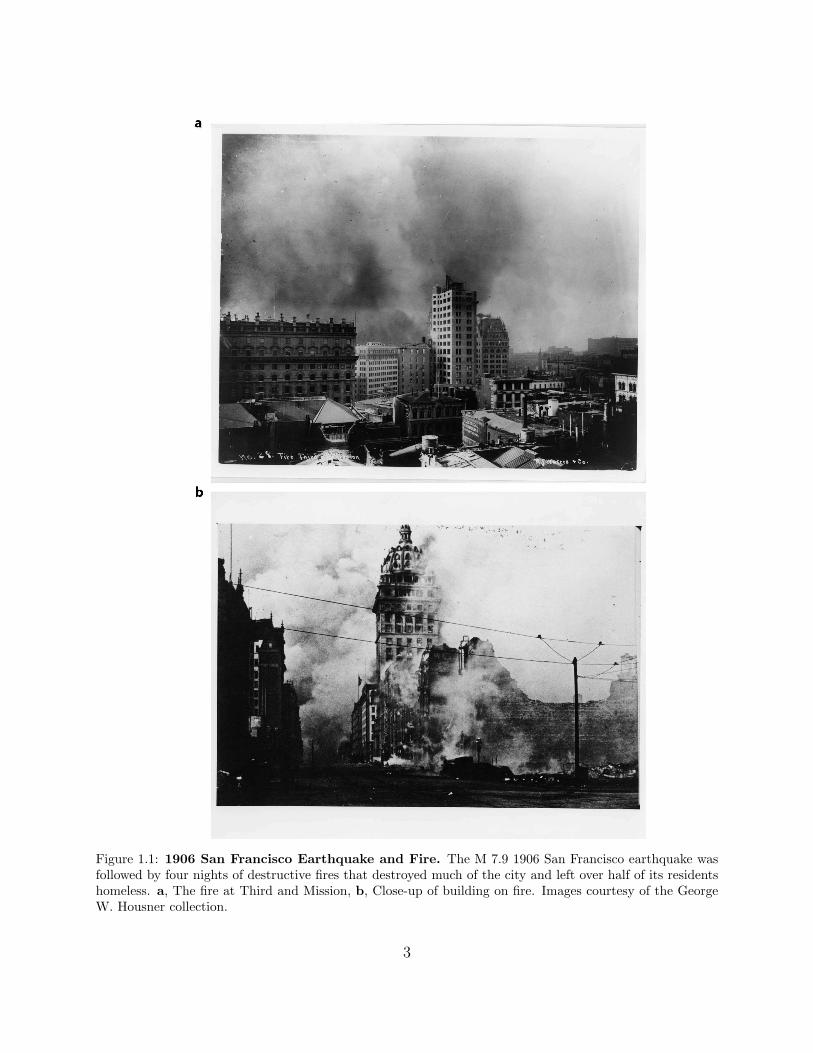
Figure 1.1: 1906 San Francisco Earthquake and Fire. The M 7.9 1906 San Francisco earthquake wasfollowed by four nights of destructive fires that destroyed much of the city and left over half of its residentshomeless. a, The fire at Third and Mission, b, Close-up of building on fire. Images courtesy of the GeorgeW. Housner collection.

3

when previous events of a similar size occurred at a given fault.

There is paleoseismic evidence that great plate-boundary earthquakes occur periodically

off the northwestern coast of the contiguous United States. This seismically active region,

called the Cascadia subduction zone, is created by the subduction of the Pacific oceanic

crust below the North American tectonic plate. Based on its shared characteristics with

other subduction zones, Heaton and Hartzell (1987) recognized the potential for the Cas-

cadia subduction zone to produce a great earthquake (of magnitude 8 or larger) or a giant

earthquake (of magnitude 9 or larger) that would result in strong shaking and large local

tsunamis. From field analysis, Atwater and Hemphill-Haley (1997) verified that about once

every five hundred years, the Cascadia fault produces a great earthquake that is followed

by a devastating tsunami. The last such earthquake happened about 300 years ago in 1700.

Goldfinger et al. (2012) found that these 500-year earthquakes are due to full-margin rupture,

and estimates the magnitude to be 9 or larger. The same study estimates the probability

of a giant earthquake in the next 50 years at 7-11% and the probability of a magnitude 8

or larger earthquake caused by rupture of the southern portion of the fault zone at 18% or

32-43%, depending on the model used.

A continental transform fault, the San Andreas fault extends for nearly a thousand miles

from its southernmost point located south of Los Angeles close to the Salton Sea, tracing

northward along the coast through San Francisco, to its northernmost point, the Mendocino

Triple Junction off the coast of Cape Mendocino in northern California. Unlike the Cascadia

fault, both moderate and large earthquakes on the San Andreas fault and its sister faults

pose a seismic threat due to their close proximity to cities in California. A number of

notable earthquakes have occurred on the San Andreas fault in the 20th and 21st century,

the largest of which is the infamous 1906 San Francisco earthquake. With an estimated

moment-magnitude of 7.9 according to Thatcher et al. (1997) and an estimated surface wave

magnitude of 7.75 according to Wald et al. (1993), the earthquake was followed by four

nights of destructive fires, documented in Figure 1.1, that destroyed much of the city and

left over half of its residents homeless. According to the 2008 UCERF (Uniform California

Earthquake Rupture Forecast) Version 2 report, the probability of a magnitude 6.7 or larger

4

-125Ê-120Ê

-115Ê -110Ê -105Ê -100Ê -95Ê -90Ê -85Ê -80Ê-75Ê

-70Ê-65Ê

25Ê

30Ê

35Ê

40Ê

45Ê

50Ê

-125Ê-120Ê

-115Ê -110Ê -105Ê -100Ê -95Ê -90Ê -85Ê -80Ê-75Ê

-70Ê-65Ê

25Ê

30Ê

35Ê

40Ê

45Ê

50Ê

-125Ê-120Ê

-115Ê -110Ê -105Ê -100Ê -95Ê -90Ê -85Ê -80Ê-75Ê

-70Ê-65Ê

25Ê

30Ê

35Ê

40Ê

45Ê

50Ê

0 500

km

-125Ê-120Ê

-115Ê -110Ê -105Ê -100Ê -95Ê -90Ê -85Ê -80Ê-75Ê

-70Ê-65Ê

25Ê

30Ê

35Ê

40Ê

45Ê

50Ê

0.010.020.030.040.060.080.100.120.160.210.270.350.460.590.771.00

SA g

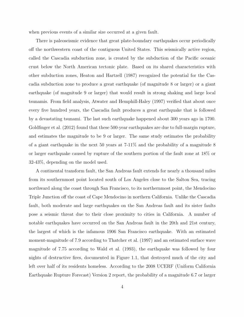
Figure 1.2: 2008 U.S. Geological Survey National Seismic Hazard Map: 1.0-Second SpectralAcceleration with 10% Probability of Occurrence in 50 Year PE, BC rock. Hazard maps, aswell as other important factors such as site soil characteristics and occupancy, are incorporated into seismicprovisions in building code. Figure courtesy of the U.S. Geological Survey.

earthquake occurring in California in the next 30 years is greater than 99%, with an average

repeat time of 5 years (Field et al., 2009). The estimated probability of a magnitude 7.0

earthquake is 94%, with an average repeat time of 11 years. The probability of a magnitude

7.5 earthquake is 46% with a repeat time of 48 years. It is only a matter of time until one of

these earthquakes occurs near a city. Fortunately, California is a seismically-proactive state,

thanks in part to programs like ShakeOut that serve to increase public awareness, professional

organizations like EERI, SEAOSC, and ASCE that bring together civil engineers, and well-

known Californian universities that advance the field of earthquake engineering.

Seismic Risk: Civil Structures

The U.S. Geological Survey (USGS) routinely publishes United States National Seismic

Hazard Maps that estimate earthquake ground motions for various probability levels, an

example of which is shown in Figure 1.2 (Petersen et al., 2008). Hazard maps, as well as

5

other important factors such as site soil characteristics and occupancy, are incorporated into

seismic provisions in building code (BSSC, 2003; ICC, 2000). Earthquake mitigation is as

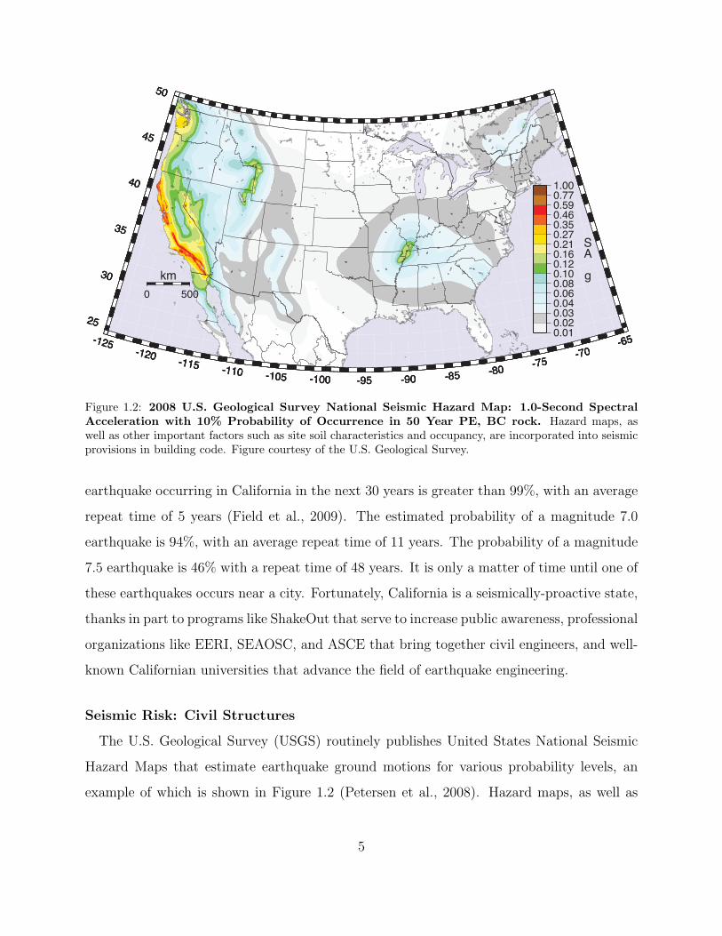
much a social and economic issue as it is an engineering issue. According to Jennings (2013) in

his book review of ‘Earthquakes and Engineers: An International History written by Robert

K. Reitherman’ and published in 2012, “the development of earthquake engineering was not

a smooth, continuous process, nor was it one always advanced by damaging earthquakes,

but rather, it was influenced by more complex interactions with society;” for example, it

wasn’t until after the M 6.4 1933 Long Beach earthquake that significant changes were made

to California’s building code. Unreinforced masonry buildings performed very poorly in the

1933 Long Beach Earthquake, some examples of which are shown in Figure 1.3 (Reitherman,

2012). Even today, adoption of a model seismic building code is uneven across and within

states, including areas with high levels of seismic hazard. In addition to the adoption of

a model code, the code must also be enforced. This is generally the responsibility of local

government building officials. Undoubtedly, public policies that mitigate seismic risk must

include steps to educate and raise public awareness in addition to developing effective land-

use regulations and building codes.

The largest seismic risk in the United States today stems from older structures that

were designed in accordance to the building code at the time of construction and have not

been retrofitted to correct for seismic vulnerabilities that were discovered post-construction.

In extreme cases, proactive measures are taken against unsafe building types or practices.

One such example is unreinforced masonry structures, whose construction was prohibited by

building codes in California in 1933. A 1986 URM Law was passed requiring local govern-

ments in Seismic Zone 4 to inventory URM buildings, establish loss reduction programs, and

report their progress and recommended that local governments establish seismic retrofit stan-

dards, adopt mandatory strengthening programs, and enact measures to reduce the number

of occupants in URM buildings (SSC, 2004). As of 2004, 25,900 URM buildings with an

average size of 10,000 square feet have been inventoried in Zone 4 regions in California, and

55% of those inventoried have been retrofitted. To put this figure into context, there were

about 12 million buildings in California in 2004.

6

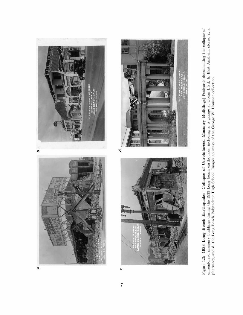
Figure

1.3:

1933

Long

Beach

Earthquake:

Collapse

ofUnre

inforced

Maso

nry

Buildings]

Postcardsdocumentingthecollapse

of

unreinforced

mason

rybuildings

duringthe1933

Lon

gbeach

earthquake,

includinga,agarage

atOceanBlvd,b,East

Anaheim

stores,

c,a

pharmacy,

andd,theLon

gBeach

Polytechnic

HighSchool.Im

ages

courtesyof

theGeorgeW

.Housner

collection.

7

Another source of seismic risk is newer structures that incorporate a novel feature such

as a structural system, material, or construction technique, whose performance has not yet

been validated by a major earthquake. Moderate-sized earthquakes can serve as canaries,

revealing problems with existing types of structures at the cost of relatively little damage

and little to no loss of life. A frequently-cited example, the 1994 Northridge earthquake

exposed the brittle nature of welded beam-column connections in steel moment-resisting

frame buildings. These connections were designed to behave as plastic hinges in the case of

heavy seismic loading, but were instead observed to have undergone brittle fracture, even in

buildings that experienced only moderate levels of shaking. A FEMA-sponsored partnership

of SEAOC, ATC, and CUREe, the SAC Joint Venture was carried out from 1994 to 2000

to develop guidelines and standards for the repair or upgrading of damaged steel moment

frame buildings, the design of new steel buildings, and the identification and rehabilitation

of at-risk steel buildings. These buildings were not found to present enough of a hazard

to warrant taking measures similar to those taken against unreinforced masonry structures,

though the building code was updated and other mitigation steps were taken.

The remainder of this chapter is comprised of the following: Section 1.1 presents a

discussion of structural damage for building types in the United States, with a focused

discussion of types of damage that can be detected using high-frequency seismograms, and

Section 1.2 contains a literature review of existing structural health monitoring and damage

detection methods.

1.1 Structural Damage

In order to assess the potential for structural health monitoring and damage detection sys-

tems for seismic mitigation, we must first understand the types of structural damage that

occur during earthquakes. Structural damage can be defined as a change to the structure

that adversely affects its performance, thereby reducing its structural integrity. Structural

damage generally weakens the structure’s vertical or lateral force-resisting-systems. Other

types of damage are classified as nonstructural. Examples include the falling of slabs from

8

a hanging ceiling or a crack propagating through stucco covering a stud wall. The general

design philosophy in the United States, similar to that used in Japan and Chile, is to prevent

collapse for larger, less frequent earthquakes, while deeming small levels of damage accept-

able for moderate-sized earthquakes that are expected to occur during the lifespan of the

structure.

The impact of recent earthquakes in Haiti, China, and Chile support the fact that build-

ings that haven’t been designed or constructed to be seismically resistant are the ones that

are most at risk from earthquakes. The M 7.0 2010 Haiti earthquake left more than 300,000

people dead and 1.3 million homeless, according to Haiti (2010). An EERI reconnaissance

team evaluated building performance in Port Au Prince and nearby areas. They found that

nearly all of the severe damage and collapse occurred in buildings that were constructed

without considering the effects of earthquakes; the majority of buildings that were designed

for earthquakes and constructed well did not collapse (DesRoches et al., 2011). The M 7.9

2008 Sichuan earthquake killed over 69,000 people and left 5 million homeless. The following

factors contributing to the poor performance of buildings: the high intensity of ground mo-

tion that was above that anticipated by Chinese seismic design code, the poor construction

quality of buildings in terms of materials and seismic design, the large number of unrein-

forced masonry buildings and similar brittle structures, the practice of using heavy solid clay

bricks for infill walls and non-structural elements, and the many structures that have large

openings at their ground floor creating a soft-story (Zhao et al., 2009).

In contrast to these earthquakes is the M 8.8 2010 Maule, Chile earthquake and tsunami,

that together resulted in over 500 deaths. Like the United States and Japan, Chile is

seismically-resilient country, with strong public policy programs and building codes that

improve seismic safety. According to Moehle and Frost (2012), “like many other economically

developed countries in the world, including the United States, Chile is also a nation of income

equality, and the 2010 Maule, Chile earthquake demonstrated both the effectiveness and the

shortcomings of modern earthquake risk reduction programs.” Most of the building damage

was contained to unreinforced masonry and adobe single-family dwellings that were built

without the assistance of a professional engineer and typically constructed of a quality to

9

withstand only the types of earthquakes experienced in the region in the past 100 years

(Astroza et al., 2012).

1.1.1 Structural Damage to Buildings in the United States

The overall seismic performance and typical seismic issues for 15 model building types (clas-

sified by the lateral load resisting system) commonly found in the United States is repeated

here from The Rapid Visual Screening of Buildings for Potential Seismic Hazards Handbook,

Version 2 (ATC, 2002).

The most hazardous building type is unreinforced masonry, and seismic issues can

stem from insufficient floor anchorage, excessive diaphragm deflection, low shear resistance,

and slender walls. Steel frame buildings with unreinforced masonry infill are also hazardous

due to the falling hazard the infill poses. When sufficiently reinforced, reinforced masonry

can perform well in moderate earthquakes, but poor construction techniques can pose prob-

lems. Another seismic hazard is the existence of older tilt-up buildings that have not been

retrofitted. While construction practices are now improved in California, older tilt-ups are

likely to have weak connections between the walls and diaphragms as well as between the

concrete panels. Failure of these connections during an earthquake can lead to collapse of

wall panels and the roof. Steel frame buildings with concrete shear walls tend to

perform well during earthquakes, and their seismic vulnerabilities include shear cracking

around openings in shear walls, wall shear failure at construction joints, and bending failure

from insufficient chord steel lap lengths. Precast concrete frames can vary widely in

performance, generally depending on the strength and ductility of the structure. Typical

seismic issues include poorly designed connections between prefabricated elements, accumu-

lated internal stresses from shrinkage, a loss of vertical support due to inadequate bearing

area, insufficient connection between floor elements and columns, and corrosion of metal con-

nectors between prefabricated elements, in addition to the problems experienced by shear

wall buildings. The best seismic performance is generally by wooden stud wall buildings

and light metal buildings due to the fact that they are lightweight and typically low-rise.

10

The most common seismic issue encountered is sliding of the building initiating from an

inadequate connection between the building and the foundation. Steel frame buildings

generally behave in a satisfactory manner due to their strength, flexibility, and lightness,

but as mentioned previously, steel moment-frames in particular are vulnerable to fracture at

welded connections.

1.1.2 1994 Northridge Earthquake: Lessons Learned

The M 6.7 Northridge Earthquake occurred at 4:31am on January 17, 1994. It resulted in the

deaths of 57 people, roughly 9,000 injuries, and cost over $24 billion (in 1994 $) in damage,

mitigation, and public assistance (not including repair costs outside of insurance coverage)

(Eguchi et al., 1998). The damage to different building types is summarized below.

Steel Frame Buildings

During the 1994 Northridge earthquake, structural damage, notably fracture of steel

frames, occurred in more than 100 buildings designed for the ground motions produced

by the earthquake (Updike, 1996). Instead of behaving as plastic hinges as they were de-

signed, the beam-column connections underwent brittle fracture that was initiated at the

weld. Reliable post-earthquake damage evaluations were made difficult by the fact that

damage to the connections was generally not accompanied by overt indicators such as dam-

age to architectural elements or permanent building drifts. Steel moment-frame buildings

had performed well in previous earthquakes, and they were a preferred building type for

seismically active areas. More than 20 such structures were subjected to and survived the

1906 San Francisco earthquake and fire; many of these buildings are still in service today

(Hamburger et al., 2009). The 1994 Northridge earthquake was “the first severe seismic field

test of modern steel structures”, and while significant problems were noted, the structures

performed as expected and no structural collapse occurred (Krawinkler et al., 1996).

The nature of the weld fracture was determined through a variety of field and labora-

tory experiments. By analyzing data from 51 moment-frame buildings that represent 330

11

inspected frames consisting of a total of 5,120 beam-to-column connections, Youssef et al.

(1995) found that about half of all of the connections at one level of the frame reported no

damage, and another third reported weld damage only. In both laboratory tests (a number

of which where conducted prior to the Northridge earthquake) and analyzed specimens that

were located in buildings impacted by the earthquake, fracture initiated in the weld metal

of the bottom flange groove weld, and the crack either remained in the weld or extended

into the column (Engelhardt and Sabol, 1997). Detailed analysis of sixteen fractured welded

connections was conducted by (Kaufmann et al., 1997). The most frequent fracture type re-

sulted in fracture which penetrated across the column flange. Other fractures were observed

to penetrate into the beam flange or the flange welds and the heat-affected zones of these

welds (Brockenbrough and Merritt, 2006). The location and source of fracture initiation was

the same for all samples, near the midwidth of the weld (near the column web centerline)

where limited access for welding results in a higher incidence of weld root incomplete fusion.

The mechanism of crack propagation in all samples was cleavage fracture. Fracture initiated

from the weld root within the weld metal.

According to SAC (2000), the issues and conditions that led to the brittle failure of

typical moment-resisting connections in Northridge were:

• The weld technique used at the bottom flange and the column flange can often result

in poor quality welding, and defects can serve as crack initiators.

• Significantly higher shear stresses than are modeled occur at the beam flanges at the

connection. The stress concentrations result in severe strength demands at the root of

the complete joint penetration welds between the beam flanges and column flanges, a

region that often includes discontinuities and slag inclusions, where cracks can initiate.

• The weld access hole that is created to ensure a continuous weld across the beam flange

leads to strain concentrations in the beam flange at the weld access hole that can lead

to low-cycle fatigue and the initiation of ductile tearing of the beam flanges.

• The restraint of motion of the steel material at the center of the beam-flange-to-column-

12

flange joint results in high stresses on the welded joint.

• The design practice of using relatively weak panel zones led to an increase in local

kinking of the column flanges adjacent to the beam flange-to-column-flange joint which

increased the stress and strain demands on the region.

• It is difficult to perform a visual inspection of welded joints, and ultrasonic testing

does not reliably detect flaws at the bottom beam flange weld root.

• In the mid-1960s, the construction industry moved to the use of a welding process and

welding consumables that produced welds with low toughness. Excessive deposition

rates, commonly employed by welders, further compromised the toughness of the weld.

Brittle fracture could initiate in welds with large defects, at stresses approximating the

yield strength of the beam steel, before ductile deformation could occur.

• For economical reasons related to the increased cost of labor, the industry began con-

structing buildings with larger members and fewer moment-connections. As member

sizes increased, strain demands, related to the span-to-depth-ratio, on the welded con-

nections also increased.

• The use of scrap-based production in steel mills in the 1980s led to beams having yield

strengths that were higher than those for previously used A36 beams. An increase

in base metal yield strength contributes to brittle behavior if the weld metal in the

beam-flange-to-column flange joints becomes under-matched.

Some of the resulting modifications made to building code in the design and welding of

moment connections include the use of cover plates and other types of connection, the use

of dogbone cutouts in the beam flanges close to the connection, the use of higher toughness

weld metals, removal of backing bars and weld tabs, and closer adherence to good welding

and inspection practices (Engelhardt and Sabol, 1997). The interested reader is directed to

‘Seismic Design of Steel Special Moment Frames: A Guide for Practicing Engineers’ which is

written for practicing structural engineers to assist in their understanding and application of

13

Excessive

Deformation

of the Panel

Zone

Fracture of Weld

Fracture at Weld

Access Hole

Excessive Deformation

of the Column Web and

Flanges

Plastic Moment

Capacity of Beam

Local Web

and Flange

Buckling

Lateral Torsional

Buckling

Figure 1.4: Typical Failure Modes for Welded-Flange-Bolted-Web Connections. This figure wasadapted from a similar figure in FEMA (2000).

the ASCE 7, AISC 341, and AISC 358 documents in steel special moment frame design. The

primary goals for special moment frame design are: 1) design for strong-column/weak-beam

configurations that distribute inelastic response over several stories; 2) design for lateral

seismic drifts that avoid the P-∆ instability under gravity loads; and 3) detailed design for

ductile flexural response in yielding regions (Hamburger et al., 2009).

A FEMA-sponsored partnership of SEAOC, ATC, and CUREE, the SAC Joint Venture,

existed from 1994 to 2000 to develop guidelines and standards for the repair or upgrading

of damaged steel moment frame buildings, the design of new steel buildings, and the iden-

tification and rehabilitation of at-risk steel buildings. The interested reader is directed to

the comprehensive set of reports and technical briefs were published by FEMA and NEHRP,

some of which are listed below:

• FEMA-350: Recommended Seismic Design Criteria for New Steel Moment-Frame

Buildings.

• FEMA-351: Recommended Seismic Evaluation and Upgrade Criteria for Existing

Welded Steel Moment-Frame Buildings.

• FEMA-352: Recommended Postearthquake Evaluation and Repair Criteria for Welded

Steel Moment-Frame Buildings.

14

• FEMA-353: Recommended Specifications and Quality Assurance Guidelines for Steel

Moment-Frame Construction for Seismic Applications.

• FEMA-355A: State of the Art Report on Base Metals and Fracture.

• FEMA-355B: State of the Art Report on Welding and Inspection.

• FEMA-355C: State of the Art Report on Systems Performance of Steel Moment Frames

Subject to Earthquake Ground Shaking.

• FEMA-355D: State of the Art Report on Connection Performance.

• FEMA-355E: State of the Art Report on Past Performance of Steel Moment-Frame

Buildings in Earthquakes.

• FEMA-355F: State of the Art Report on Performance Prediction and Evaluation of

Steel Moment-Frame Buildings.

• NEHRP Seismic Design Technical Brief No. 1: Seismic Design of Reinforced Concrete

Special Moment Frames: A Guide for Practicing Engineers.

• NEHRP Seismic Design Technical Brief No. 2: Seismic Design of Steel Special Moment

Frames: A Guide for Practicing Engineers.

In order to determine if a building has sustained connection damage it is necessary

to remove architectural finishes and fireproofing and perform detailed inspections of the

connections. As physical inspection of these connections in buildings is an expensive, ob-

trusive, and time-consuming process, FEMA offers reimbursements for preliminary post-

earthquake assessment for eligible structures with pre-Northridge welded beam-column con-

nections (FEMA, 2007). Most steel moment-frame buildings constructed during the period

1960-1994 employed connections of a type that is vulnerable to brittle connection fracture,

making them vulnerable to upcoming earthquakes.

15

Other Building Types

Other building types generally performed as expected, with the earthquake presenting

an opportunity to validate retrofitting practices for wooden, masonry, and concrete build-

ings. Reinforced concrete shear-wall buildings performed well with respect to life safety and

prevention of collapse (Osteraas et al., 1996). Retrofitted nonductile concrete frames also

performed adequately. Except for parking structures, post-1967 buildings that relied on

shear walls or ductile frames for their lateral load-resisting system performed well. How-

ever, there were indications that lateral deformation requirements of gravity columns are

inadequate to prevent potential failure. Modern parking structures with precast elements

underwent much more damage than expected, with a general pattern of failure of columns

that in some cases led to collapse. Tilt-up buildings, especially older ones, suffered a lot of

damage in the Northridge earthquake. Of the 1,200 tilt-up buildings in the San Fernando

Valley, over 400 had significant structural damage, including partial roof collapse and col-

lapse of exterior walls (CSSC, 1994). There was a high monetary value to the amount of

damage to wooden buildings, but little loss of life. The damage was generally due to poor

design and construction practices, with buildings with soft-stories or cripple walls suffering

the most damage (Hall et al., 1996). Retrofitted masonry buildings performed well, while

unreinforced masonry buildings suffered extensive damage. As seems to have been too fre-

quently the case, ‘neither the distinction between life safety and control of monetary loss nor

the probable variability of performance among buildings is well understood by the general

public’ (Somers et al., 1996).

1.1.3 Using High-Frequency Seismograms for Damage Detection

High-frequency seismograms have the potential to be used for damage detection in struc-

tures where the presence of damage results in the generation of high-frequency signals.

High-frequency generally refers to frequencies above the predominant modal response of the

structure, although this may depend on the context. High-frequency signals can occur at the

moment damage occurs, as in the acoustic emission that occurs during crack propagation.

16

High-frequency signals can also occur after damage has been created, as in the case of an

opening and closing crack, known as a ‘breathing crack.’ From an analysis of the literature,

two potential applications for damage detection using high-frequency seismograms include

the detection of weld fracture in steel moment-resisting frame buildings, and the continu-

ous monitoring of high-frequency signals in structures exposed to extreme conditions, such

as bridges, which tend to have higher-frequency sources than buildings due to traffic and

environmental loading.

There is some support in literature for the idea that high-frequency signals can be used

for damage detection in sparsely instrumented steel moment-frame buildings. Rodgers and

Mahin (2007) conducted both numerical and experimental testing on a one-third scale, two-

story, one-bay steel moment frame. On the experimental structure, twelve accelerometers

were installed, and the data were recorded with a time step of 0.01 s. The authors found

that short-duration high-frequency signals are present in acceleration records at the moment

of fracture, with the time of the fracture determined from beam-end strain gauges. The

sign of the high-frequency signal was found to be consistent with that predicted by the

equations of motion and analysis, and the high frequency content and amplitude of these

signals made them easily distinguishable from the predominant response of the structure to

shaking. According to Rodgers et al. (2007), fracture damage causes ‘sudden’ changes in

local stiffness and deflected shape, ‘sudden’ changes in global acceleration, and a ‘sudden’

release of energy in the form of elastic waves. In a separate study, the authors analyze data

collected from 24 buildings following the Northridge earthquake and use the presence of

transient signals in the acceleration records as well as other information about the buildings

to determine if weld fracture occurred, with a 67% success rate.

17

1.2 Structural Health Monitoring and

Damage Detection Methods

Structural health monitoring can be defined as the measurement of the operating and load-

ing environment and the critical responses of a structure to track and evaluate symptoms of

operational incidents, anomalies, and/or deterioration or damage indicators that may affect

operation, serviceability, or safety reliability (Aktan et al., 2000). The basic idea behind

structural health monitoring is that the dynamic properties of a structure are a function of

its physical properties, and changes in the physical properties of the structure, including the

introduction of structural damage, can lead to changes in its dynamic properties. By moni-

toring the behavior of a civil structure over time, its dynamic properties can be monitored

and used to assess its structural integrity. In the event of detected changes in its dynamic

properties, the level of damage can be assessed in what is typically formulated as an inverse

problem.

The nature of structural damage can be linear (i.e., the material properties of the struc-

ture change, however the response of the structure remains linear-elastic) or nonlinear (i.e.,

loose connections that rattle, or a crack in a beam that opens and closes based on its bending

configuration) (Doebling et al., 1996). According to Rytter (1993), a robust damage detec-

tion method should be able to: Level 1) identify damage, Level 2) localize damage, Level 3)

assess the level of damage, and Level 4) assess the consequence (e.g., give information about

the actual safety of the structure given a certain damage state).

The key components of a structural health monitoring system include the type of exci-

tation (forced or ambient), the physical quantities to be measured (e.g., modal values and

temperature), the number and types of sensors (e.g., accelerometers, fiber-optic cables, strain

gauges, anemometer, etc.), data acquisition system, and data processing. Methods of ac-

tively exciting a structure include forced vibration with a (hydraulic, mechanical eccentric

mass, or electrodynamic) shaker, impact excitation with an impact hammer, step relaxation

using a tensioning device such as a cable, or a hydraulic shake table (Sohn et al., 2004).

18

Ambient excitation is defined as the excitation experienced by a structure under its normal

operating conditions, which can consist of forces from traffic, wind, and microseisms.

While there is a wealth of research in the field of structural health monitoring, there has

been a seemingly slow adoption of these methods in industry. This may, in part, be due to

a misconnect between the developers of SHM methods and the intended users. Researchers

generally focus on the technical aspects of the problem, such as how to locate damage from

limited information, and in most studies a damage detection method is tailored to a single

building. On the other hand, building owners are generally concerned with the financial

aspects of damage detection, such as knowing information about the likelihood of damage,

cost of repair, and extension of serviceability. There is clearly room for incorporation of

structural health monitoring and damage detection methods into seismic risk management,

assessment, and mitigation. This topic is beyond the scope of this thesis. However, one

potentially high-impact application for SHM could be the monitoring of national highway

bridges. As of 2011, of the total 605,102 highway bridges in the U.S., Moore (2013) rates

67,526 (11 %) as structurally deficient and (13 %) as functionally obsolete.

Only damage detection methods which have relevance to this thesis are mentioned below.

Extensive reviews of structural health monitoring methods have been presented by Sohn et al.

(2004), Doebling et al. (1996), Doebling et al. (1998), and Friswell (2007).

1.2.1 Vibration-Based Techniques

The term ‘vibration-based techniques’ is loosely defined to include methods that rely on

changes in the global vibration characteristics of the structure, including modal frequencies,

mode shapes, and changes in measured flexibility/stiffness coefficients for structural health

monitoring and damage assessment. Most of the literature encompasses vibration-based

techniques that are typically applied to numerical or small-scale experimental cases.

Generally only the lowest modes are excited under ambient conditions. According to

Friswell (2007), an advantage to using low-frequency vibration measurements is that low-

frequency modes are generally global, and few vibration sensors are typically needed to

19

be installed on the structure to monitor these modes. The downside is that the spatial

wavelengths of the modes are typically far larger than the extent of the damage. This results

in a low spatial resolution in damage identification schemes. On the other hand, using high-

frequency excitation uses highly local modes that are able to locate damage, but only in a

close proximity to the sensor and actuator.

1.2.1.1 Natural Frequency Based Methods

Damage detection methods that rely only on changes in the natural frequencies of a structure

are inherently limited for a few reasons (Doebling et al., 1996). Foremost, natural frequencies

typically have low sensitivity to various types of structural damage, and either very precise

measurements of frequency or very large levels of damage are required to detect damage.

Even when these conditions are met, other factors (e.g., changes in the material properties

of the structure caused by changes in weather, or changes in the mass of the structure) may

be responsible for observed changes in natural frequencies.

In this case, the forward problem consists of calculating frequency shifts from a known

type of damage; the inverse problem consists of calculating the damage parameters from the

measured frequency shifts. Though multiple frequency shifts can provide spatial information

about structural damage, damage localization that relies solely on modal frequencies is diffi-

cult as there is often an insufficient number of frequencies with significant enough change to

uniquely determine the location of damage. One common method is to develop a sensitivity

relation, whereby a linear relation is developed between the natural frequencies (or changes

in natural frequencies) and physical quantities in the model, such as changes in stiffness.

1.2.1.2 Mode Shape Based Methods

Some commonly-applied techniques that are based on changes in mode shape make use of

the Modal Scale Factor (MSF), Modal Assurance Criterion (MAC), and Coordinated Modal

Assurance Criterion (COMAC). Mode shape derivatives, i.e., curvature, are also used, as

they exhibit a direct relationship to bending strain for beams, plates and shells (Doebling

20

et al., 1996). Methods based on changes in mode shapes are generally combined with outlier

methods, forward modeling using a known type of damage, or model updating.

Modal Scale Factor

A suitable scalar-based method of comparison for two mode shape vectors is to plot each

pair of elements in the mode shape vectors, on an x-y plot (Ewins, 2000). The slope of the

best straight line is called the modal scale factor, and it is defined as (for reference modal

vector φ):

MSF (ψ, φ) =ψT φ̄

φT φ̄,

where φ̄ denotes the complex conjugate of φ. If the mode shapes are similar, they should

lie close to a straight line. If the mode shape vectors are mass-normalized, this straight line

should have a slope of 1. if the points lie close to a straight line with a slope that is not one,

then one of the mode shapes is not mass-normalized or there is scaling error in the data.

Modal Assurance Criterion

The modal assurance criterion (MAC), is a simple tool used commonly in the fields of me-

chanical and aerospace engineering to provide a measure of consistency (degree of linearity)

between estimates of a modal vector. The modal assurance criterion is defined as a scalar

constant relating the degree of consistency (linearity) between one modal vector and another

reference modal vector as follows:

MAC(ψ, φ) =|ψT φ̄|2

(φT φ̄)(ψT ψ̄). (1.1)

The modal assurance criterion ranges in value from zero to one. If its value is close to one,

it is an indication that the modal shape vectors are consistent. If other explanations can be

ruled out (i.e., the modal vectors have been incompletely measured, are primarily coherent

noise, or are the result of a forced excitation other than the desired input), then it can be

assumed that the modal vectors represent the same modal vector with different arbitrary

21

scaling (Allemang, 2003). Allemang (2003) further points out that the modal assurance

criterion is most sensitive to large differences.

The partial modal assurance criterion (PMAC) is defined as a spatially limited version

of the modal assurance criterion where only a subset of the modal vector is used.

Coordinated Modal Assurance Criterion

The COMAC technique is based on the same principle as the MAC and is essentially a

measure of the correlation between the reference and the measured mode shapes for a given

common coordinate (Marwala, 2010). The coordinated modal assurance criterion (COMAC),

for the nth mode shape recorded at themth receiver, attempts to identify which measurement

degrees-of-freedom contribute negatively to a low value of MAC:

COMAC[m] =

∑

N

n=1ψnmφ̄

nm

(

∑

N

n=1ψnmψ̄

nm

)(

∑

N

n=1φnmφ̄

nm

) .

If the mode shape vectors are used then the COMAC becomes a vector.

1.2.1.3 Flexibility/Stiffness Based Methods

The flexibility matrix is defined as the inverse of the static stiffness matrix, and it relates

the applied static force to the resultant displacement. Each column of the flexibility matrix

represents the displacement of the structure to a unit force applied at the associated degree-

of-freedom. Analogously, as the stiffness matrix relates the applied force to the displacement

of the model, each column of the stiffness matrix represents the amount of force that must

be applied to the model to maintain a unit displacement at the corresponding degree of

freedom.

The formulation of the flexibility matrix is approximate in the case that not all of the

modes of the structure can be measured. Typically, only the lowest frequency modes are

measured, related to the tendency of the source to consist of lower-frequency energy. The

flexibility is most sensitive to changes in the lower frequency modes of the structures due

to its inverse relationship to the frequencies; the stiffness matrix is most sensitive to the

22

highest frequencies. Damage is detected by using modal values to compute the flexibility or

stiffness matrix of a potentially damaged structure, and comparing these values with those

determined when the structure was in an undamaged state.

1.2.1.4 Parameter Estimating and Updating

In model identification methods, a model for the structure is formulated, and static or dy-

namic data is used to update model parameters such as natural frequencies, mode shapes,

mass, stiffness, and damping matrices. Generally a constrained optimization problem based

on the equations of motions, the nominal model, and the measured data is used. Damage

detection, localization, and estimation of severity is generally performed by comparing the

updated values to the nominal values. The procedure is generally to: 1) identify an ob-

jective function, 2) define constraints, and 3) define a numerical scheme to implement the

optimization.

Matrix updating methods that use a closed-form direct solution to compute the damaged

model matrices or the perturbation matrices are known as optimal matrix update methods.

The problem is generally formulated as a Lagrange multiplier or penalty-based optimization.

Methods that are based on the solution of a first-order Taylor series that minimizes an error

function of the matrix perturbations are known as sensitivity-based update methods. Some

common objective functions include: 1) the modal force error, with constraints that preserve

the matrix symmetry of the perturbation matrices, sparsity, and positive-definiteness, 2) the

mean-squared-error computed in the time domain, 3) the mean-squared error computed in

the frequency domain using the transfer function.

Damage detection techniques using finite element model updating often leads to updating

of a large number of damage parameters, especially when the structure has many structural

members (Sohn et al., 2004). There are techniques that can help with solving for a large

number of system or damage parameters, e.g., the Hamiltonian Markov chain method has

been shown to aid in solving higher-dimensional Bayesian model updating problems (Cheung

and Beck, 2009).

23

1.2.2 Acoustic Methods

Acoustic damage detection methods typically rely on the comparison of a recent signal to

an archived baseline response function, known as a template. The template is recorded at

a time when the structure is undamaged. The sensor network must have a high sampling

rate to capture the propagation of waves throughout the structure. Acoustic techniques have

been explored experimentally and numerically for thin plates and beams (Park et al., 2007;

Wang et al., 2004; Wang and Rose, 2003), which serve as waveguides that effectively carry

information from the location of structural damage to a receiver. This information, namely

differences in waveform and amplitude between the current signal and the template, are used

to diagnose damage.

Acoustic methods can be passive or active, and sensor networks can be permanently

installed or temporary. Giurgiutiu and Cuc (2005) reviews current techniques, including

embedded ultrasonic non-destructive evaluation (NDE), which uses a transmitter to interro-

gate the structure while a receiver records the structural response. 1) Pitch-catch: a pulse is

emitted by a transmitter and travels through the material to a receiver. Differences in guided

wave shape, phase, and amplitude are used to detect damage in the medium between the

transmitter and receiver. 2) Pulse-echo: a pulse is emitted by a transmitter, which also acts

as a receiver to detect damage in the form of additional echoes. 3) Time-reversal: a signal

sent by a transmitter arrives at a receiver, where the signal is time-reversed and reemitted.

Structural damage that causes linear reciprocity to break down leads to discrepancy between

the original signal and the final signal received by the transmitter. 4) Migration: recorded

waves are back-propagated through the material by systematically solving the wave equation

to image reflectors in the medium.

1.2.2.1 Guided-Wave Methods

Guided-wave testing is an active form of structural health monitoring that relies on a network

of sensors and actuators to probe the structure with a controlled high-frequency vibration.

The vibration excites stress waves that essentially become trapped within nearby structural

24

members, such as beams or plates, hence the term “guided wave.” A baseline response,

recorded when the structure is known to be in an undamaged state, serves as a reference

signal to which future responses, when the structure is not known to be undamaged, can be

compared. Features that potentially indicate damage are extracted from the recorded signal,

typically by removing the baseline response from the recorded response in the time-domain

or in the time-frequency domain. Finally, a chosen technique (e.g., a neural network coupled

with an FEM model or seismic migration) is used to detect and locate damage and estimate

its severity. A review of guided-wave structural health monitoring methods is presented by

Raghavan and Cesnik (2007).

A transducer is a device that converts a signal of one form of energy into another form of

energy. The most popular types of transducers used in guided-wave testing are piezo-electric

and can act as both sensors, which detect vibration by converting a mechanical signal into an

electrical signal, and actuators, which generate vibration by converting an electrical signal

into a mechanical signal. Other types of transducers are also available, including those based

on fiber optic, microelectromechanical (MEMS), and nanotube technologies.

The two main techniques used to produce vibration are dubbed “pulse-echo” and “pitch-

catch.” In pulse-echo setups, the sensor is co-located with the actuator, and in pitch-catch

setups, the sensor is located away from the actuator. Differences between a recorded signal

and a prerecorded baseline are used to detect damage. In pulse-echo setups, damage is

detected by the presence of additional features in a signal that are caused by waves reflecting

off a damaged region, such as a crack, which acts as a reflector. In pitch-catch setups,

damage is detected by changes in the recorded signal from the baseline signal that could

denote damage in the medium between the actuator and sensor. A time-reversal method is

experimentally verified by Park et al. (2007) with an experimental setup that consists of a

pair of piezoelectric patch transducers that are attached to a composite plate. In the first

step of the method, a Lamb wave is emitted by the first transducer. The signal recorded

at the second transducer is time-reversed and retransmitted by the second transducer. The

resulting signal recorded at the first transducer is compared to the initially emitted Lamb

wave. The Lamb wave is designed, using Mindlin plate theory, in such a way that the

25

reconstructed signal will be very close to the emitted signal. Nonlinearities between the two

transducers that are due to damage should result in differences between the original emitted

signal and the final resulting signal. This method bypasses the need for a prerecorded

baseline.

For most applications, a dense network of actuators and sensors is needed for damage

localization (e.g., multiple actuators and sensors located on each plate). Furthermore, most

studies take place in a laboratory setting, and the robustness of these systems still need to be

vetted in situ against the noisy conditions that would be encountered on an actual structure.

Finally, many of these methods are based on theoretical formulations for simple geometries,

such as a simply supported plate. However, in the real world, these elements would be likely

fixed to other members, and hence they would have radically different boundary conditions

than those considered in lab. For these reasons, these methods are not yet industry-ready.

1.2.3 Time-Frequency Signal Analysis

There are two basic approaches to time-frequency analysis. The first is to divide the signal

into slices in time and to analyze the frequency content of each of these slices separately

(e.g., Wigner-Wille transform). The second is to filter the signal at different frequency

bands and window the frequency bands to analyze their energy content as a function of time

and frequency. Other time-frequency analysis techniques include, but are not limited to,

wavelet analysis, and empirical mode decomposition combined with Hilbert transform (Sohn

et al., 2004). Time-frequency analysis can aid in damage detection by better distinguishing

a damage signal temporally and spectrally.

1.2.3.1 Analytic Signal

The analytic signal (also known as analytic representation or analytic associate) xa(t) of a

real-valued signal x(t) is defined as

xa(t) = x(t) + iH{x(t)} ,

26

where the Hilbert transform H{x(t)} of a signal x(t) is given by:

H{x(t)} = F−1 {(−isgnf)F{x(t)}} .

The negative frequency components of real signals are superfluous, as X(−f) = X∗(f)

for f > 0, where X(f) is the Fourier transform of x(t). By converting to the analytic signal,

the negative frequency components are set to zero with no loss of information, but at the

expense of transitioning to a complex-valued signal.

1.2.3.2 Time-Frequency Distributions

Boashash (2003) presents a comprehensive reference of time-frequency signal analysis, and

two time-frequency distributions discussed in the book are summarized here. Generally

speaking, the time-frequency distribution ρxa(t, f) of the analytic signal xa(t) aims to repre-

sent the energy, temporal, and spectral characteristics of xa(t) in the (t, f) plane. By using

the analytic signal rather than the real-valued signal when constructing a time-frequency dis-

tribution, spurious terms caused by interference between the positive- and negative-frequency

components can be avoided.

Spectrogram

A spectrogram can be used to analyze the time-varying spectrum of frequencies in a

signal, effectively estimating the energy density of the signal in the time-frequency plane

by partitioning the signal in the time domain and analyzing the frequency content of each

window.

The spectrogram is constructed from a signal x(τ) and a chosen time-limited, real, even

window w(τ) by multiplying the signal by a window centered at time τ = t and taking the

squared magnitude of the Fourier transform of the resulting signal;

Sw

x (t, ω) = |Fτ−>ω {x(τ)w(τ − t)} |2.

27

There is a trade-off between time and frequency resolution in accordance with the ‘un-

certainty relationship.’ Using a shorter window w(τ) allows for better localization of the

spectrum in time, but also makes for a decrease in resolution in frequency. Using a longer

window w(τ) allows for better resolution of the signal in frequency, at the expense of a poorer

localization of the signal in time.

Wigner-Ville Distribution

The Wigner-Ville distribution of an analytic signal xa(t) is given by:

Wxa(t, ω) = Fτ−>ω {xa(t+ τ/2)x∗a(t− τ/2)} .

According to Boashash (2003), the Wigner-Ville distribution has a number of advantages,

including but not limited to the following: realness, time-shift invariance, frequency-shift

invariance, time marginal (integration over frequency gives the instantaneous power), fre-

quency marginal (integration over time gives the energy spectrum), and preservation of the

instantaneous frequency and time delay. Its limitations include the artifacts, or cross-terms,

which appear midway between multicomponent signals.

1.2.4 Other Methods

Other inspection methods, such as visual inspection, magnetic particle inspection, radiog-

raphy, eddy current, ultrasonic, and thermal field are not covered here. Neither are aerial

and satellite methods that detect post-disaster damage at the scale of an entire city or re-

gion. Machine learning methods, such as neural networks, have also not been touched upon;

although the main disadvantage to using this approach is the lack of experimental training

data, there has been some recent success in applying pattern recognition to acoustic emission

signals obtained from databases of empirical data (Friswell, 2007). Finally, hybrid techniques

have not been mentioned. However, a hybrid SHM system is the most promising as each

method has its own strengths and weaknesses, and augmenting a vibration-based technique

with a high-frequency time-domain technique could make for a more robust detection of

28

damage.

1.2.5 Validation and Comparative Studies

There is a (fortunate) lack of seismic data recorded in instrumented U.S. civil structures that

were structurally damaged during an earthquake. This is due to the absence of a recent large

earthquake in the United States, the ability of structural engineers, improvements in building

codes and seismic design maps, and the relatively small percentage of densely instrumented

buildings. Without a wealth of real-world data for validating and benchmarking damage

detection methods, numerical and experimental testing are key in providing insight and

direction for developing structural health monitoring and damage detection methods.

1.2.5.1 Publicly-Available Datasets for the Purpose of Benchmarking

There exist a few publicly-available datasets for the purpose of validating and benchmarking

structural health monitoring, particularly damage detection methods. These datasets, as

well as the methods that have been used to study them, are summarized below.

The most extensively-studied SHM benchmark was created by the International Asso-

ciation for Structural Control (IASC) of the American Society for Civil Engineers (ASCE)

structural health monitoring task group. The benchmark problem was carried out in two

phases, Phase I (a numerical study) and Phase II (an experimental study).

IASC-ASCE SHM Benchmark: Phase I

A special issue on Phase I of the IASC-ASCE Structural Health Monitoring Benchmark

to date was published in the Journal of Engineering Mechanics (Volume 130, Issue 1, pp.

1-104). The issue contains a brief introduction by Bernal and Beck (2004) of the benchmark

and methods applied to the Phase I benchmark problem in the special issue, a description

of the benchmark problem by Johnson et al. (2004), as well as seven papers each presenting

the application of an SHM technique to the benchmark problem (Bernal and Gunes, 2004;

Caicedo et al., 2004; Hera and Hou, 2004; Lam et al., 2004; Lus et al., 2004; Yang et al.,

29

2004; Yuen et al., 2004). The results published in these papers and other studies subsequently

performed on the benchmark problem are discussed below.

Phase I of the IASC-ASCE SHM benchmark problem is described in detail by Johnson

et al. (2004) and is summarized here for convenience. The numerically-modeled structure

used for the benchmark is a four-story, two-bay by two-bay steel-frame quarter-scale structure

(2.5 m by 2.5 m plan and 3.6 m height) located at the Earthquake Engineering Research

Laboratory at the University of British Columbia. Damage is introduced either to a diagonal

brace (by reducing the stiffness or removing the brace) or to a beam-column connection (by

changing the connection from a moment connection to a simple connection).

Participants in the benchmark are tasked with detecting damage using a 12-DOF shear

building as the identification model. Data is numerically simulated using either a 12-degree-

of-freedom or a 120-degree-of-freedom analytical structural finite-element model. Using two

models to generate the data provides participants with a means of studying modeling error.

The output “noise level” is the RMS of the sensor noises, generated using independent

Gaussian pulse processes, as a percentage of the maximum RMS acceleration responses; the

noise level is 10% for the benchmark problem. Six different cases are considered by varying

the excitation source (wind or shaker), model used to generate the data (12 DOF or 120

DOF), and number of sensors (accelerometers) used for the output.

Six different damage patterns are considered, and they are defined as:

Damage Pattern I: No stiffness in the braces of the first story.

Damage Pattern II: No stiffness in any of the braces of the first and third stories.

Damage Pattern III: No stiffness in one brace in the first story.

Damage Pattern IV: No stiffness in one brace in the first story and in one brace in the

third story.

Damage Pattern V: The same as damage pattern iv, but with a floor beam at the first

level partially unscrewed so that the beamcolumn connection can only transmit forces

and cannot sustain any bending moments.

30

Damage Pattern VI: Two-thirds stiffness, i.e., a one-third stiffness loss in one brace in

the first story.

The six cases are defined as:

Case 1: 12-DOF model used to generate data, symmetric mass distribution on roof, ambient

excitation, both a known and unknown input, Damage Patterns I and II.

Case 2: 120-DOF model used to generate data, symmetric mass distribution on roof, am-

bient excitation, both a known and unknown input, Damage Patterns I and II.

Case 3: 12-DOF data generation model, symmetric mass distribution with a shaker diago-

nal on roof, unknown input for the data, Damage Patterns I and II.

Case 4: 12-DOF data generation model, asymmetric mass distribution, shaker excitation,

unknown input, Damage Patterns I, II, III, IV, and VI.

Case 5: 120-DOF data generation model, asymmetric mass distribution, shaker excitation,

unknown input, Damage Patterns I, II, III, IV, V, and VI.

Case 6: 120-DOF data generation model, asymmetric mass distribution, shaker excitation,

unknown input, limited sensors to those on the second and fourth floors, Damage

Patterns I, II, III, IV, V, and VI.

Yuen et al. (2004) apply a two-stage method that is based on a modal identification

technique and model parameter updating using a Bayesian model identification method.

In the first stage, the MODE-ID modal identification procedure is used to estimate modal

parameters from the response data when the structure is in either an undamaged or a possibly

damaged state. In the second stage, the estimated modal parameters are used in a Bayesian

model updating method to determine the most probable values of the stiffness parameters.

Yuen et al. (2004) note that in all of the benchmark cases, the damage can be identified

solely on the basis of the maximum posterior value of the stiffness parameters, however the

authors recommend that the probability of damage in each story instead be calculated as a

31

probability of the fractional reduction in interstory stiffness. The damage probability curves

are also presented in the study. The uncertainty in estimating the damping ratios is much

higher than in estimating the natural frequencies, and in the case of an unknown excitation,

additional information, such as the spectral level of excitation, is needed to better identify

the damping ratios. Only the (lower) modes that contribute significantly to the motion

can be identified. The reduction in accelerometers resulted in larger uncertainties of the

estimated stiffness parameters, as well as a few spurious increases in stiffness and false

positives (estimated decreased stiffnesses in undamaged floors). Yuen et al. (2004) note that

in the event that the “known” mass matrix is inaccurate, significant bias can be introduced

in the resulting estimates. By relaxing the conditions on the mass matrix to include some

uncertainty, robustness is gained at the expense of a small loss of precision.

A single-step Bayesian modal identification approach is considered by Lam et al. (2004).

The basic concept is to identify a set of optimal model parameters based on maximizing

the posterior probability density function (PDF) for the parameters, which is a product of

the prior PDF for the parameters as well as a PDF giving the probability of the spectral

data given some values for the parameters. The excitation is assumed to be wide-band and

able to be modeled as white noise. First, spectral estimates are formed from the cross-

correlations of the responses. A subset of the spectral estimates, i.e., a range within a

specified frequency band, is used for parameter estimation using a Bayesian approach. The

estimated parameters include the model stiffness parameters as well as the modal parameters

(modal frequencies, damping ratios, mode shapes, modal forcing spectral density terms, and

the covariance matrix of the prediction error). The posterior probability distribution function

of the parameters is formulated. It incorporates the subset of the spectral data and the prior

probability distribution function for the stiffnesses and is maximized in a single-step to yield

the most likely estimates for the parameters. According to Lam et al. (2004), unlike a two-

step minimization, a one-step minimization ensures that the structural model corresponding

to the optimal stiffness parameters is the optimal structural model within the chosen class

of models. The methodology did not fail to detect damage in any of the benchmark cases

considered, although in some cases the identified damage extent was slightly overestimated

32

for cases with modeling error, often within the margin of statistical error.

Caicedo et al. (2004) estimate interstory stiffness values by applying the natural excitation

technique (NExT) method, in conjunction with the eigensystem realization algorithm (ERA)

and a least squares optimization. The modal parameters are estimated by applying ERA to

cross-correlation functions, which are computed from the forced vibration data and treated

as free vibration data. This technique is applicable for problems in which the excitation is

broadband and random, and the ratio of masses is known. There is some art in choosing the

reference signal, which cannot lie at a node at any of the considered modes. This method

was found to be robust to noise, modeling error (Case 2), and coupling due to asymmetry

in the mass distribution (Case 4), with typical errors in the identified stiffness values for

the members less than 1%. For Case 6, as half of the sensors were removed, an iterative

procedure was used to estimate the eigenvectors and stiffness terms. The approach provides

an indication of the location of the damage, but may include some false positives, which

indicate that damage occurs in some locations where damage is not present. The authors

note that when an iterative approach is used, a single sensor would be adequate to determine

the eigenvectors, eigenvalues, and stiffnesses of the structure. If the number of sensors is

limited, this technique could be applied by independently relocating the available sensors on

a structure while keeping the reference channel at the same position.

A flexibility-based method is employed by Bernal and Gunes (2004) to locate and quantify

damage. The method consists of the following steps: 1) compute the state-space realization

from the measured signal, 2) extract the flexibility matrices from the matrices of the real-

ization (using the ERA-OKID algorithm when the input is known and the Sub-ID subspace

technique when the input is stochastic), 3) compute the change in flexibility from the un-

damaged to the damaged state, 4) apply the damage locating vector (DLV) technique to

localize the damage, and 5) quantify the damage. The steps of DLV localization is as fol-

lows: 1) compute the change in flexibility, 2) obtain a singular value decomposition of DF, 3)

compute the stresses in an undamaged model of the structure, 4) reduce the internal stresses

in every element to a single characterizing stress, 5) compute the svn index, 6) check if the

svn index is lower than a threshold value, 7) compute the normalized stress index vector, 8)

33

compute the vector of weighted stress indices, and finally 9) the weighted stress indices that

are less than 1, which include the potentially damaged elements. Arbitrary viscous damping

is considered. The authors further partitioning the shear beam into four sections per floor in

an attempt to locate damage at the element level. When there are at least three sensors per

level one can dene the interstory stiffness and center of stiffness positions from the modal

data and use the changes in these quantities to determine the level, location, and extent of

the damage without the need for an explicit model. The authors note that the approach

may not be robust in eld conditions, because the truncation of the modal space is likely to

be too large to allow accurate computation of the physical parameters.

Lus et al. (2004) apply a two-step approach that consists of finding a first-order minimal

state space realization of the system using only the input-output measurements, and then

extracting the physical parameters (mass, damping, and stiffness parameters) of the under-

lying second-order system. An Observer/Kalman filter identification (OKID) algorithm is

used to identify the Markov parameters of the system, which are used in the eigensystem re-

alization algorithm to realize the discrete-time first-order system matrices. The initial state

space model is further refined by minimizing the output error between the measured and

predicted response using a nonlinear optimization approach based on sequential quadratic

programing techniques. Finally, the physical parameters of the FE model are determined

from the state-space model, and damage is determined by comparing these values with those

recorded when the structure was in an undamaged state.

Two time-frequency analysis methods are applied by Yang et al. (2004) to detect the

occurrence of damage spikes as well as changes over time in the structure’s modal properties

(frequencies and damping ratios). The first method, based on filtering using the empirical

mode decomposition (EMD), is used to to extract high-frequency damage spikes that occur at

the instant that damage occurs. Structural damage results in a sudden change of structural

stiffness that causes a discontinuity in acceleration in the vicinity of the location of damage.

Yang et al. (2004) found that for Damage Patterns I and II, the damage spikes can always be

detected when the measured data has zero or little added noise. A Monte Carlo simulation

is performed for ten sample cases, and it is estimated that the probability of detecting the

34

damage spike, with 10% noise added, is about 30%. The authors note that there is some art

in choosing the intermittency frequency, i.e., the cutoff frequency for filtering, which should

be above the modal frequencies but below the frequency of the damage spike. As the damage

spike is only present in the acceleration records on the damaged floors in this study, it is

relatively simple to qualitatively determine the floor at which the damage occurred. For

Damage Patterns III, IV, and V, the damage spikes are submerged with the noise in the

y-component sensor data. The authors conclude that the detection of damage time instants

and damage locations through the identification of damage spikes is influenced significantly

by the severity of damages and the noise-to-signal ratio. The second method, a Hilbert-

Huang approach based on the EMD and Hilbert transform, is combined with the random

decrement method to determine the natural frequencies and damping ratios of the structure

before and after damage. The authors note that only a single record is needed to determine

these modal values, but a full array of sensors should be installed in order to identify the

damage locations.

A wavelet-based technique is used by Hera and Hou (2004) to detect damage spikes in the

acceleration data. The supplied MATLAB program for the benchmark problem is slightly

modified to introduce damage in the middle of a response history by piecing together two

segments of response data, one directly before damage, one directly after damage, while

satisfying continuity conditions in velocity and displacement. In this example, even when

all diagonal braces are broken between two floors, damage spikes are only observed in the

acceleration records immediately above and below that floor. Localization of damage to a

story is achieved using patterns in the spatial distribution of spikes. Hera and Hou (2004) find

that the effectiveness and reliability of the proposed approach depends on damage severity

and measurement noise level. One advantage to this technique is that it is not dependent

on knowledge of the structure’s modal response and only relies on the spatial distribution of

sensors. However, structural information may still be needed in order to properly interpret

the results from the wavelet analysis. Although the severity of damage was seen to have a

predictable change on the amplitudes of the spikes, the authors did not present a way of

quantifying the severity of damage depending on the data.

35

Later studies published on Phase I of the IASC-ASCE benchmark study include a two-

stage eigensensitivity-based finite element model updating method by Wu and Li (2006)

and a method based on the change of strain energy in each structural element in both the

damaged and undamaged state by Sharifi and Banan (2008).

IASC-ASCE SHM Benchmark: Phase II and Phase IIe

Phase II consists of experimental testing of the model located at the Earthquake Engineer-

ing Research Laboratory at the University of British Columbia (UBC). The experimental

setup is described by Dyke et al. (2003) and is summarized here for convenience. The 4-story

2-bay by 2-bay (2.5 m x 2.5 m x 3.6 m)steel-frame (grade 300W steel) scale model is located

at the Earthquake Engineering Research Laboratory at the University of British Columbia

(UBC). Acceleration data is recorded using three sources of excitation (ambient vibrations,

impact hammer tests, and electrodynamic shaker tests), with nine cases of damage simu-

lated by removing bracing within the structure or by loosening bolts connecting beams to

columns. The benchmark provides a great example for the comparison of the numerical data

with the experimental data, and a common framework (dataset and objectives) with which

to accurately compare the performance of different SHM and DD methods.

Ching and Beck (2004) apply a two-step probabilistic structural health monitoring ap-

proach; the modal parameters and their uncertainties are estimated in the first step, and

they are used in the second step to determine the probability that stiffness reductions ex-

ceed a prescribed damage threshold. In the cases where damage is simulated by removing

braces, all damage was successfully detected with both the hammer excitation or the ambi-

ent vibration excitation. No false alarms were detected using hammer excitation, but some

false detections were found using ambient vibration excitation. In cases where damage is

introduced by loosening the bolts connecting beams to columns, only the hammer excitation

data were considered for determining the mode shapes, as they had the best quality. Most

damage cases were detected, but there were many false detections, most likely due to the

difficulty of estimating the rotational stiffness as the stiffness matrix of the structure was

found to be dominated by the columns.

36

IMAC Benchmark

An earlier benchmark problem was initiated at the 15th International Modal Analysis

Conference (IMAC XV), and consisted of numerical data simulating a finite element model

of a one-third scale steel frame structure subjected to uncorrelated shaker inputs at its

roof (Black and Ventura, 1998). Three different damage configurations (including one blind

example) were created by removing members or changing member properties, and 5% noise

was added to the output signals, 16 acceleration time-histories. One damage detection study

was published on this dataset, in which the Damage Index Method was applied to localize

and estimate the level of damage (Park et al., 1998).

Center of Structural Monitoring and Control at the Harbin Institute of Tech-

nology Benchmark I and II

Finally, a real-world benchmark problem was recently made available by the Center of

Structural Monitoring and Control (SCM) at the Harbin Institute of Technology using data

recorded on an instrumented cable-stayed bridge in China (Li et al., 2010, 2012, 2013). First

opened to traffic in 1987, the bridge is one of the first built cable-stayed bridges in mainland

China. According to Li et al. (2013), the bridge was repaired between 2005 and 2007 for

cracks observed at the bottom of a girder segment over the mid-span, and corroded stay ca-

bles (especially those near the anchors). During this time, the bridge was also upgraded with

an SHM system that includes more than 150 sensors, including 14 uniaxial accelerometers, 1

biaxial accelerometer, an anemoscope, a temperature sensor, and optical fiber Bragg grating

sensors. Two benchmark problems are proposed, based on the bridge. The first benchmark

problem is to assess the condition of the stay cables based on the strains measured over the

period of one week in January, 2008 and the fatigue properties of the deteriorated steel wires

as determined from fatigue testing on some specimens taken from the cables near the bottom

anchorages. Specifically, researchers are asked to assess the fatigue life prediction model of

parallel wire cables, as well as the residual fatigue life assessment of deteriorated cables. The

second benchmark problem is to detect, localize, and quantify damage using acceleration

measured from January to August 2008. Li et al. (2013) presume that the bridge was dam-

37

aged gradually over this time period by overloading. The benchmark study is a blind test,

as no further information about the damage is supplied. Lastly, a finite-element model has

also been made available for this benchmark problem. As this benchmark problem was only

recently made available, no papers have yet been published on this dataset.

1.2.5.2 Datasets Used in this Thesis for the Purpose of Validation

In this thesis, numerical testing, small-scale experimental testing, and full-scale experimental

testing is conducted for the purpose of developing and testing damage detection methods for

civil structures instrumented with a seismic array. In Chapter 2, a novel damage detection

method that relies on approximating connection fracture as a hammer blow is experimentally

tested using a small-scale steel frame. Experimental impact hammer data is also obtained

in an instrumented steel moment-resisting-frame building. In Chapter 3, an instrumented

small-scale experimental shear beam is subjected to a repeatable pulse at its base using a

shake table. The experiment is repeated with the beam in different damage configurations.

A novel damage detection method, that relies on the detection of repeating high-frequency

short-duration pulses, is successfully applied to the structure. Numerical studies in Chapter 4

further investigate the feasibility of the proposed damage detection method for weld fracture,

as well as exploring a time-reversed reciprocal method for a frame. Finally, high-frequency

data from the SCM benchmark bridge in China, as well as a test bed data set using a

nonlinear frame provided by the Los Alamos National Laboratory are studied in Chapter 5.

In the Appendix, experimental data from a densely-instrumented high-rise building located

in Osaka is used to obtain the impulse response function of the building. A numerical model

is developed, based on the design parameters for the structure, and is subsequently damaged

and studied.

38