Damage Detection in a Smart Beam using its Vibrational...

Columbia International Publishing Journal of Vibration Analysis, Measurement, and Control (2015) Vol. 3 No. 2 pp. 93-112 doi:10.7726/jvamc.2015.1005

Research Article

______________________________________________________________________________________________________________________________ *Corresponding e-mail: [email protected] 1 Indian Institute of Technology, Roorkee (India).

93

Damage Detection in a Smart Beam using its Vibrational Response

Himanshu Kumar1*, S C Jain1, and Bhanu K Mishra1

Received: 18 April 2015; Published online 25 July 2015 © The author(s) 2015. Published with open access at www.uscip.us

Abstract In this paper, the flexure vibrations in a smart beam, fixed at one end have been studied. The beam is having surface crack in a transverse direction. The smart material used is PZT-5H (Lead Zirconate Titanate). Here analytical technique for detection of damage and its severity is presented and is verified in the rectangular cross- section beam. Using free Vibrational analysis and applying FEM, first three Vibrational frequencies and mode shapes of the un-cracked and cracked beam has been evaluated. Effect of crack location and crack depth over the first three natural frequencies has been analyzed. It is reported that, for a cantilever beam case, damage can be identified by analyzing the changes in first three values of natural frequencies, except when the crack is located near the node of the chosen vibration mode. Later after validation, these frequencies are also used as input in the neural network A comparative study is done with the previous research work in the same field, and it is found that the error has been reduced in finding the crack location and crack depth. This approach can be applied in on line health monitoring in complex structures, off shore structures and space structures. Keywords: Damage Detection; Damage Localization; Neural Network; Health Monitoring; Vibration Analysis

Notation S Strain Components (Unit m/m) T Stress Components (Unit N/m2) D Displacement Components (Unit C/m2) E Electric Field Components (Unit N/C) s Compliance coefficients (Unit m2/N) c Stiffness Coefficients (Unit N/m2) d Piezoelectric coupling coefficients for strain-charge form (Unit C/N) e Piezoelectric coupling coefficients for stress-charge form (Unit C/m2) g Piezoelectric coupling coefficients for strain-voltage form (Unit m2/C) q Piezoelectric coupling coefficients for stress-voltage form (Unit N/C)

Himanshu Kumar, S C Jain, and Bhanu K Mishra / Journal of Vibration Analysis, Measurement, and Control (2015) Vol. 3 No. 2 pp. 93-112

94

e

Piezoelectric stress coefficient

E Electric field fs Surface force intensity Fs Overall Surface force l: Length of Beam h: Distance of crack from fixed end b: Height of beam w: Crack Depth l1: Length of beam covered by PZT patch. (h/l): Crack Location Ratio (CLR) (w/b): Crack Depth Ratio (CDR) Є Strain field Є xx Normal strain in x direction Єs Shear strain σ Stress field σxx Stress in x direction υ Poisson ratio ω Frequency

1. Introduction The life and reliability of structures can be affected by structural ageing, environmental circumstances and reuse. This may lead to structural damage such as cracks. Cracks present a serious threat to the proper performance of structures. Most of the failures in the structures can be traced to fatigue cracks. For this reason, much research has been done on identification of crack location and depth using modal frequency parameters of the structures. A crack occurring in a structural element causes a local variation in stiffness, affecting the dynamic behavior of the structure to a considerable degree. The objective of any damage assessment problem is to identify whether structural damage has occurred, and if so, to determine the location and extent of the damage. The common structural health-monitoring techniques are based on the modal characteristics of a structure. This paper is aimed to present analytical technique for detection of damage and its severity.

By using the terms Detection and severity we mean finding the location and size of crack in a structure. Here a beam case has been taken for the demonstration purpose of this technique. Here the approaches used are energy and artificial neural network (ANN) approach. The first systematic investigations on damage detection using vibration information appeared in the 1970s. Doebling (1999) attributes the initial developments in this field to the offshore oil industry, while Dimarogonas et al. (1990) acknowledges the power generation industry for the first studies on the more specific problem of crack identification over the years, methods for damaged detection incorporated more sophisticated information as they become available both from laboratories and computer simulations. In fact, it was not until the late 1970s that more systematic investigations on natural frequency shifts, many of which including finite element models, appeared in scientific publications, and only in the 1980s did changes in mode shape changes and related quantities start to be considered as potential damage indicators.


95

Damage diagnosis based on changes in natural frequencies was the first, vibration-based method to appear in the literature, and to date they remain by far the most investigated. Cawley and Adams (1979) published what, is usually referred as the first systematic attempt to detect damage from changes in natural frequencies Dimarogonas et al. (1990) studied the flexural vibrations of a cantilever beam with rectangular cross-section having a transverse surface crack extending uniformly along the width of the beam and obtained analytical results and relate the measured vibration modes to the crack location and depth. Quin et al (1990) presented an FEM based approach where element stiffness matrix of a beam with a crack is first derived from an integration of stress intensity factors, and then a finite element model of a cracked beam is established. Stubbs et al. (2005) further developed the sensitivity approach to also include better estimates of damage severity using fractional changes of the natural frequencies as damage indicators. Scott Whitney (1999) presented work on vibrations of cantilever beams for PZTs. Kam & Lee (1994) presented a paper over crack detection, using frequency and strain energy approach. They presented an energy method for identifying the size of a crack at given location in structures using one measured Eigen couple. Friswell et al. (2002) also extend Cawley and Adam's ideas with the introduction of statistical analysis for the identification of the best damage scenario. Recently using modern approaches such as neural networks by Luo and Hanagud (1997), and genetic algorithms by Friswell et al, (2002) has been applied in this area. Using free Vibrational analysis and applying Finite Element Method, some Vibrational frequencies and mode shapes of the uncracked and cracked beam has been evaluated. These frequencies are validated using experimental methods.

2. Smart Materials Piezoelectrics are the most popular smart materials. They undergo a deformation when an electric field is applied across them, and conversely produce voltage when strain is applied.

Fig. 1. 3-D model of sample Smart Beam, used for analysis


96

1

23

E3

Fig. 2. Representation of PZT Patch, used in the Smart Beam

In fig. 1 the smart beam has been shown. The axes for PZT (fig. 2) are identified by numerals: 1 corresponding to X-axis, 2 corresponding to Y-axis and 3 corresponds to Z-axis. The four possible forms for piezoelectric constitutive equations are given below. The name for each of the forms is arbitrary. Strain-Charge Form: S = sE .T + d

t.E (1)

D=d.T + ЄT.E (2)

Here the matrix d contains the piezoelectric coefficients for the material, and it appears twice in the constitutive equation (the superscript t stands for matrix-transpose).

Stress- Charge Form

T = cE.S – et.E (3)

D = e.S + ЄS.E (4)

Strain-Voltage Form: S = sD.T + g

t.D (5)

E = -g.T + ЄT-1

.D (6)

Stress- Voltage Form T = cD.S – q

t.D (7)

E = -q.S + ЄS-1

.D (8)

During the work, the smart material used was PZT-5H, with the following physical properties: Crystal Symmetry Class: Uniaxial; Density: 7730 kg/m3; d31 = -274 e -12 m/V; d32 = -274 e -12 m/V; d33 = 593 e -12 m/V; Relative permittivity = 3400.

3. Modal Analysis


97

We use modal analysis to determine the natural frequencies and mode shapes of a structure. Here the discretized beam is multi degree of freedom system with no damping. So an Undamped Multi-Degree of Freedom free vibration case has been analyzed. Here in this analysis we found natural frequencies of vibration and their associated modes, without regard to which of them may be important in application or how motion is initiated. Without damping, all d.o.f. moves in phase with one another and at the same frequency ω. Natural frequencies in a linear problem are independent of {Dst}. However, nonstructural mass that may be associated with static loads must be represented in [M]. Nodal displacements and accelerations associated with vibration are

{D} = {D} sin ωt and _..

2{ } { }sinD D t (9)

With damping matrix [C] omitted, and using the above equations we yield,

For Undamped free vibration: _

2([ ] [ ]){ } {0}K M D (10)

Here ω2 is an eigenvalue, and ω is a natural frequency. Matrix 2[ ] [ ]K M is called a dynamic

stiffness matrix. A physical interpretation of vibration comes from writing Eq. 1 & 2 in the form as follow:

[ ]K_

{ }D = ω2 _

[ ]){ }M D (11)

It says that a vibration mode is a configuration in which elastic resistances are in balance with inertia loads. Let {D} contain only degree of freedom that may assume nonzero values after all rigid-body modes and mechanisms (if any) are suppressed. Thus [K] is positive definite. If element mass matrices are consistent, or lumped with strictly positive diagonal coefficients, [M] is also positive

definite. Then the number of nonzero ωi is equal to the number of degree of freedom in_

{ }D .

Occasionally two or more ωi are numerically equal. Then their associated vibration modes _

{ }iD are

not unique, but mutually orthogonal modes for the repeated ωi can be established. Type of element used for the problem is shell element. SHELL181 element available in ANSYS has been used for the modeling of complete smart structure, cracked and un-cracked.

4. Finite Element Model

ANSYS is a software package, used for analysis of structural, fatigue and vibrational analysis. Here we used ANSYS 8.0 version for the analysis of the Smart beam system. As the problem comprises of crack and PZT patches also, the element taken is 4 node finite strain shell element, which is available in ANSYS as SHELL181 (Fig. 3).


98

Fig. 3. Smart Beam discretized in Finite Elements

This element has been used for the modeling of cracked beam and PZT patch. SHELL181is suitable for analyzing thin to moderately-thick shell structures. It is a 4-node element with six degrees of freedom at each node (Fig. 4):

a) Translation in x, y, z Directions, and

b) Rotations about the x, y, and z-axes.

SHELL181 is well-suited for linear, large rotation, and/or large strain nonlinear applications. Change in shell thickness is accounted for in nonlinear analyses. In the element domain, both full and reduced integration schemes are supported.

Fig. 4. Four (4) Node Shell Element Geometry

In order to validate the Finite Element Model prepared for the analysis, the very basic parameter i.e. natural frequencies of the beam obtained from the ANSYS software package have been compared with the theoretically obtained values.

For the beam material used in the present work: E=206 E09Pa A=400 E-06 ρ =7650 Kg/m3 l = 0.3 m, Using the formulae, the natural frequencies found are as given in table 1:

Table 1 Validation of First Three Natural Frequencies Mode Theoretical

Value(Hz) Reference

Paper(Hz) [6] Finite Element

Model(Hz) Difference of FE Model

with Theoretical Difference of FE Model

with reference paper[6]

1 183.89 185.20 183.74 0.08157 % 0.78834 %

2 1152.39 1160.0 1146.1 0.54582 % 1.19827 %

3 3226.81 3259.10 3192.8 1.05398 % 2.03430 %


99

On comparing these results, we find that the difference in the frequencies obtained theoretically with those obtained from the finite element model is very less (<1.1 %) for first three modes. It validates the finite element model prepared for the analysis. Using the finite element model, first three natural frequencies and mode shapes for the cracked beam with the change of crack location and crack depth have been obtained. These results have been validated experimentally and also with the previous work of Kam & Lee (1994). Fig. 5 shows a cracked beam we can see the location and depth of crack. Here the notations are as follow:

h l

bw

l1

Fig. 5. Schematic representation for crack location and crack depth

l: Length of Beam h: Distance of crack from fixed end b: Height of beam w: Crack Depth l1: Length of beam covered by PZT patch. (h/l): Crack Location Ratio (CLR) (w/b): Crack Depth Ratio (CDR) The first three natural frequencies of a cracked beam for different crack sizes and crack depths have been obtained. 4.1 Variation of First Natural Frequency with Variation in CDR & CLR The variation of first natural frequency of the beam Vs crack depth for different crack locations and Vs Crack Locations for different Crack Depths is given in fig. 6 and fig. 7. The first Natural frequency decreases as the crack depth increases; however as the location of crack move away from the fixed end, this variation becomes less.


100

Variation of Ist Natural Frequency with CDR

100

110

120

130

140

150

160

170

180

190

0 0.05 0.1 0.15 0.2 0.25 0.3 0.35 0.4 0.45 0.5

Crack Depth Ratio(CDR)

Natu

ral

Fre

qu

en

cy(H

z)

CLR = 0.1

CLR = 0.3

CLR = 0.5

CLR = 0.7

CLR = 0.9

Fig. 6. Variation of 1st natural frequency Vs crack Depth

Variation of 1st Natural frequency Vs Crack

Location

130

140

150

160

170

180

190

0 0.2 0.4 0.6 0.8 1Crack Location Ratio(CLR)

Natu

ral

Fre

qu

en

cy (

Hz)

CDR = 0.1

CRD = 0.2

CDR = 0.3

CDR = 0.4

CDR = 0.5

Fig. 7. Variation of 1st natural frequency Vs crack Location

4.2 Variation of Second Natural Frequency with Variation in CDR & CLR The variation of 2nd natural frequency Vs crack depth for different crack locations is plotted in the fig. 8. As far as this variation is concerned, we can say that for the 2nd natural frequency, the percentage variation is less as compared with the variations of 1st natural frequency. This variation is less and keeps on decreasing for the crack located at far end from the fixed end.


101

Variation of IInd Natural Frequency with CDR

900

925

950

975

1000

1025

1050

1075

1100

1125

1150

0 0.05 0.1 0.15 0.2 0.25 0.3 0.35 0.4 0.45 0.5

Crack Depth Ratio(CDR)

Na

tura

l F

req

ue

nc

y (

Hz)

CLR = 0.1

CLR = 0.3

CLR = 0.5

CLR = 0.7

CLR = 0.9

Fig. 8. Variation of 2nd natural frequency Vs Crack Depth

Variation of IInd Natural frequency with CLR

900

950

1000

1050

1100

1150

0 0.1 0.2 0.3 0.4 0.5 0.6 0.7 0.8 0.9

Crack Location ratio (CLR)

Natu

ral

freq

uen

cy (

Hz)

CDR= 0.05

CDR= 0.1

CDR= 0.15

CDR= 0.2

CDR= 0.25

CDR= 0.3

CDR= 0.35

CDR= 0.4

CDR= 0.45

CDR= 0.5

Fig. 9. Variation of 2nd Natural Frequency Vs crack Location

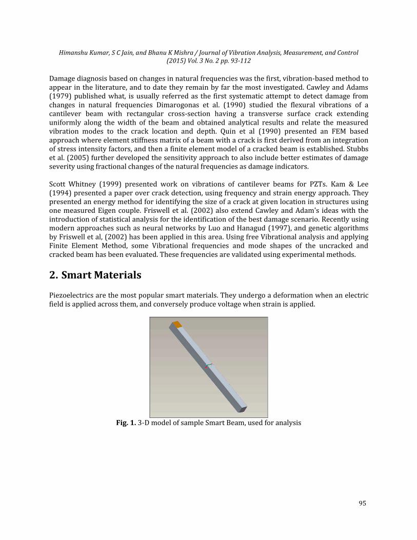
The variation of 2nd natural frequency Vs crack location is plotted in the fig. 9. Here the variation has been plotted for different crack depths. 4.3 Variation of 3rd Natural Frequency with Variation in CDR & CLR The variations of 3rd natural frequency Vs crack depth for different crack locations is plotted in fig. 10 and natural frequency Vs crack location for different crack depths have been plotted in the fig. 11.


102

Variation of 3rd Natural Frequency Vs Crack

depth

2500

2600

2700

2800

2900

3000

3100

0 0.05 0.1 0.15 0.2 0.25 0.3 0.35 0.4 0.45 0.5

Crack depth ratio(CDR)

natu

ral F

req

uen

cy

(Hz) CLR = 0.1

CLR = 0.3

CLR = 0.5

CLR = 0.7

CLR = 0.9

Fig. 10. Variation of 3rd Natural Frequency Vs Crack Depth

Variation of 3rd Natural Frequency with CLR

2500

2550

2600

2650

2700

2750

2800

2850

2900

2950

3000

3050

3100

0 0.1 0.2 0.3 0.4 0.5 0.6 0.7 0.8 0.9

Crack Location Ratio (CLR)

Na

tura

l F

req

ue

nc

y(H

z)

CDR = 0.05

CDR = 0.1

CDR = 0.15

CDR = 0.20

CDR = 0.25

CDR = 0.30

CDR = 0.35

CDR = 0.40

CDR = 0.45

CDR = 0.50

Fig. 11. Variation of 3rd Natural Frequency Vs Crack Location

5. Experimental Setup and Analysis The experimental set up prepared for the study of Vibrational behavior of uncracked and cracked structure consists of the following major parts. 1. PZT Patches. 2. Piezo Sensing System. 3. Piezo Actuation System. 4. Data Acquisition Card 5. Data Processing Machine. The patches of smart material for the experiment are of size 0.040 * 0.020 * 0.001 m3. Piezo sensing system consists of charge to voltage converting signal-conditioning amplifier with variable gain. Individual input/output connectors are provided for connecting PZT crystal. As for Piezo actuator drive unit, it is a four channel drive unit, with the frequency range of 10-1000 Hz. The interface card used is National Instruments USB-8451 device. It is a high-speed USB-based device used to communicate to serial peripheral interface (SPI) and inter-integrated circuit (I2C) compatible

http://sine.ni.com/nips/cds/view/p/lang/en/nid/202368


103

devices. The NI USB-8451 includes driver software that provides high level, easy-to-use Lab VIEW functions, property nodes, and references. Beam samples have been prepared by machining them and preparing cracks of different sizes. The cracks have been generated by using 1 mm precise hack-saw, in workshop.

Fig. 12. Smart Beam mounted on Experimental set up test stand

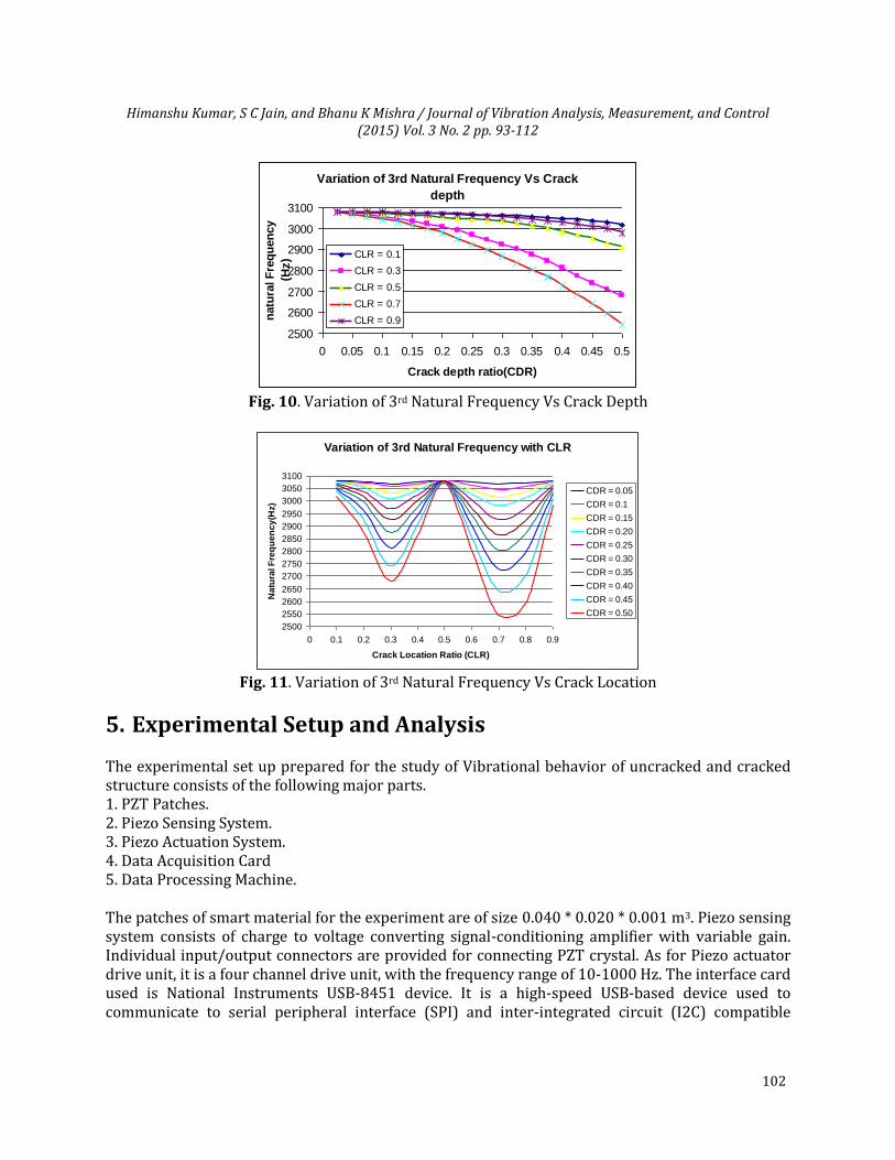
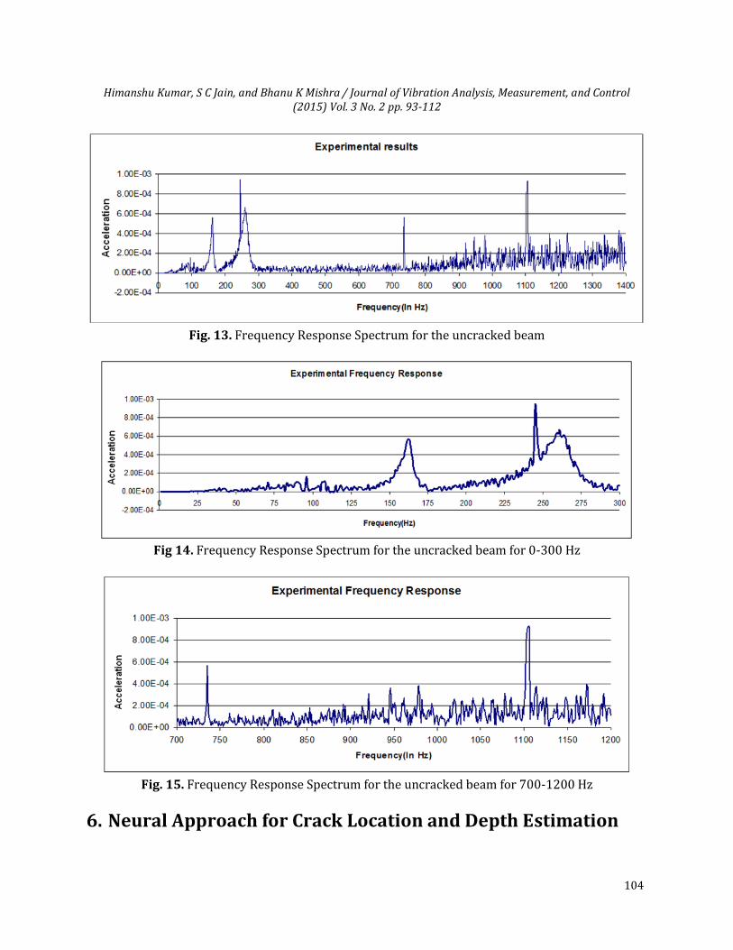
In fig. 12 the beam (uncracked), mounted over beam stand can be seen. Here two PZT patches have been glued to the beam, one each for sensing and actuation. The smart beam has been connected to the sensing and actuation system, using terminal box. During Modal analysis of the beam, the beam was mounted in a stand and the PZT patch, working as a sensor was glued at the fixed end. An impulse loading was applied at the free end of the beam. The response generated by this impulse loading was sensed through sensor and after processing this signal, the results were analyzed over LAB-View software. For the analysis of cracked beam, the crack in the beam was simulated by a thin saw cut of width 1 mm. This is in line with the procedure followed by Cawley and Ray (1979). Crack of size 10 mm was made in a beam of size 20*20mm at mid location. The uncracked and cracked beams were subjected to experimental modal testing and measured vibration frequencies were extracted from frequency response spectrum. Fig. 13 shows the Frequency domain analysis of the beam vibrations. The response has been plotted for the frequency range of 0-1400 Hz. For better analysis of the spectrum it has been zoomed, and two important ranges, containing 1st and 2nd natural frequencies are plotted in fig. 14 and fig. 15 with the frequency range of respectively 0-300 and 700-1200 Hz. This response for the uncracked beam, indicate resonance at some frequencies, for example: 162.5 Hz, 264 Hz, 734 Hz and 1108 Hz. During Finite Element analysis, it has been observed that the beam is also having some out of plane frequencies at 273 Hz, 732 Hz Etc. So Out of these four resonances or modal frequencies, 162.5 and 1108 Hz are the desired first and second modal frequencies i.e. natural frequencies for flexure mode of vibration.


104

Fig. 13. Frequency Response Spectrum for the uncracked beam

Fig 14. Frequency Response Spectrum for the uncracked beam for 0-300 Hz

Fig. 15. Frequency Response Spectrum for the uncracked beam for 700-1200 Hz

6. Neural Approach for Crack Location and Depth Estimation


105

In this paper, the artificial neural network approach has been applied to find the location and size of crack. An artificial neural network operates by creating connections between many different processing elements, each analogous to a single neuron in a biological brain. These neurons may be physically constructed or simulated by a digital computer. Each neuron takes many input signals, then, based on an internal weighting system, produces a single output signal that's typically sent as input to another neuron.

Fig.16. Artificial Neural Network representation

The earliest kind of neural network is a single-layer perceptron network, which consists of a single layer of output nodes; the inputs are fed directly to the outputs via a series of weights. In this way it can be considered the simplest kind of feed-forward network. The sum of the products of the weights and the inputs is calculated in each node, and if the value is above some threshold (typically 0) the neuron fires and takes the activated value (typically 1); otherwise it takes the deactivated value (typically -1). Other class of networks consists of multiple layers of computational units, usually interconnected in a feed-forward way. Each neuron in one layer has directed connections to the neurons of the subsequent layer. The analytically computed modal frequency parameters for various crack locations and depths using a fracture mechanics based crack model, are used as input in the artificial neural network. Using these inputs, network was trained to identify both the crack location and depth. The roots of the transcendental equation (βn) are related to the natural frequency (ωn) as follows [10]:

2

n n

EI

A

(12)

Where n is the mode number, E the Young’s modulus of the beam material, I the cross sectional moment of inertia, ρ the mass per unit length and L the length of the beam. The above formulation gives frequencies of a cracked beam for varying crack locations and depth. Since for a given beam the value of the expression under the square root sign in the above equation is fixed, we can normalize the frequency as shown below:


106

2nn

EI

A

(13)

Thus βn is a measure of the frequency of the cracked beam. The normalized frequency can be used for training and testing the neural networks for crack identification. Though a beam modeled as a continuous system has infinite modes, the first few modes are the most important and easily measured. 6.1 Important Steps for Neural Network Analysis The following steps are used to obtain the optimal network configuration such that the mean square error for training (MSETE) and mean square error for testing or generalization (MSEGE) are less than the prescribed value: Step 1. Select a network with a minimal configuration. Step 2. Train the network until MSETE < μ, where μ is a small positive real number. Step 3. Calculate MSEGE. Step 4. If MSEGE > μ then increase the number of hidden nodes or vary the number of layers and go to step 2. Else stop. This process is repeated until MSETE and MSEGE are less than a certain prescribed value (μ = 0.001). The value of μ is selected on the basis of previous studies, as Suresh S. (2004) has taken it as 0.02. In the present work, μ=0.001 has been taken Hence the results of the present work are expected to be more refined.

In the present work two different networks have been investigated. As shown in fig. 17, the first network has a single layer. Number of neurons in the layer was varied from 4 to 20. For each simulation 50 runs were conducted. It is observed from fig. 18 and fig. 19 that the MSEGE is least for the case of 16 neurons, but still it is more then desired i.e. MSEGE > 0.001. So there is no use of increasing neurons. Hence another network with two hidden layers has been applied.

β1

β2

β3

h/l

w/b

Crack Depth

Crack Location

Neural Network

N1

Fig. 17. Block Diagram for Single Layer Network


107

Mean Square Error(MSE) Curve

0.029

0.031

0.033

0.035

0.037

0.039

0.041

0.043

0 4 8 12 16 20 24

Neurons

Err

or

Epochs = 5000

Epochs = 1000

Fig. 18. MSE for Crack Locations

Mean Square Error (MSE) Curve

0.002

0.0025

0.003

0.0035

0.004

0.0045

0.005

0.0055

0 4 8 12 16 20 24

Neurons

Err

or

Epochs = 1000

Epochs = 5000

Fig. 19. MSE for Crack Depths

β1

β2

β3

h/l

w/b

Crack Depth

Crack Location

Layer 1 With

16

Neurons

Layer 2 With

8 Neurons

Fig. 20. Block Diagram for Multi Layer Network

Fig. 20 shows a schematic modular neural network diagram for the Multi Layer Perceptron Network with two hidden layers. Here the results are presented for few epochs, although the analysis has been undertaken for epoch ranging from 500 to 10000, with increment of 500 epochs. The Mean square error and correlation factor value for both Crack Length Ratio and Crack Depth Ratio are presented in fig 21 and fig. 22 in graphical form. We can see here that for the Multi Layer Perceptron Network with two hidden layers, MSEGE (Mean Square Error) < 0.001, for epochs >7500 for both the Crack Location Ratio and Crack Depth Ratio.


108

Mean Square Error for Multi Layer Network

0

0.001

0.002

0.003

0.004

0.005

0.006

0.007

0.008

0.009

0.01

0 2000 4000 6000 8000 10000

Epoch

MS

E

MSE for Crack

Location Ratio

MSE for Crack Depth

Ratio

Fig. 21. MSE for different Epoch

Correlation Factor for Multi Layer Network

0.915

0.92

0.925

0.93

0.935

0.94

0.945

0.95

0.955

0.96

0.965

0 2000 4000 6000 8000 10000

Epoch

Co

rrela

tio

n f

acto

r

For Crack Location

Ratio

For Crack Depth

Ratio

Fig. 22. Correlation Factor for different Epoch

The table 2 gives the optimum parameters for Multi Layer Perceptron Network with two hidden layers.

Table 2 Optimum Parameters for Multi (2) Layer Perceptron Network Network Initialization Model Neural Network

Inputs 3 (β1, β2 & β3)

Outputs 2 (w/b, h/l)

Error Goal 1 x 10-3

Layers 02

Neurons [16] – [8]

No. of Runs 200

The results obtained from the Multi Layer Perceptron Network with two hidden layers with the above listed network parameters are presented in the next section.

6.2 Results of Multi-Layer Perceptron Network with Two Hidden Layers


109

The network was trained till the desired limits of MSEGE were achieved. Afterwards the network was cross validated and tested with data set unused during the training phase. As given in previous papers from Seresh S. et.al. (2004), the best way of dividing the data for the Neural Network analysis, is in the ratio of 65%, 25% and 10%. Here the same ratio has been used in deciding number of inputs for the network. Data taken for various processes are as follow: Training: 20 Inputs; Cross Validation: 40 Inputs; Testing: 20 Inputs. The results of analysis, done for multi layer perceptron are given in table 3, fig. 23 and fig. 24. Here we have tested various neural networks, with varying numbers of neurons in both the layers. For Example, a network listed as “[x] –[y]” represents a network with ‘x’ neurons in first layer and ‘y’ neurons in second layer. We can see that, for 10000 epochs, the network with [16] - [8] combination of neurons, gives the desired values of MSEGE, i.e. MSEGE <0.001. So we have selected [16] – [8] network for final analysis. In the fig. 23 and fig. 24, the X-axis represents different Networks, with symbolic representation of 1, 2, 3….

Mean Square Error Curve for MLP with 5000

epoch

0

0.001

0.002

0.003

0.004

0.005

0 1 2 3 4 5 6

Layers with Different values of neurons

Err

or

Crack Location Ratio

Crack Depth Ratio

Fig. 23. MSE for MLP with 5000 Epochs

Mean Square Error Curve For MLP with 10000

Epoch

0

0.0005

0.001

0.0015

0.002

0.0025

0.003

0.0035

0.004

0 1 2 3 4 5 6Layers with Different Values of Neurons

Err

or

Crack Location Ratio

Crack Depth Ratio

Fig. 24. MSE for MLP with 10000 Epochs


110

Table 3 Comparison of MLP network results with the previous paper.

Actual Values RMS Error from Current work(In Percentage)

RMS Error from Reference Paper of Suresh S. et. Al (2004) (In Percentage)

C D R C L R Depth Location Depth Location 0.15 0.4

0.6 25.09 7.403 3.765 7.578 0.8

0.25 0.4 0.6 10.0044 5.3897 10.496 7.003 0.8

0.35 0.4 0.6 5.25 0.977 4.837 12.808 0.8

0.45 0.4 0.6 2.3268 2.71 9.361 11.682 0.8

Table 4 Output from the MLP network

Actual Values MLP Output Error

Crack Depth Ratio

Crack Location

Ratio

Crack Depth Ratio

Crack Location

Ratio

Depth Location

% RMS % RMS

0.15

0.2 0.120633 0.17874 19.57829 25.09 10.63012 7.403 0.4 0.127523 0.361925 14.98493 9.518833 0.6 0.153725 0.588435 2.48329 1.927565 0.8 0.215456 0.827583 43.6371 3.44782

0.25

0.2 0.247161 0.181265 1.135474 10.0044 9.367704 5.3897 0.4 0.247051 0.379485 1.179492 5.128686 0.6 0.237256 0.60124 5.097771 0.20667 0.8 0.298198 0.811586 19.2791 1.44824

0.35

0.2 0.374959 0.201225 7.1311 5.25 0.61231 0.977 0.4 0.374149 0.402881 6.89962 0.72015 0.6 0.351049 0.592848 0.29984 1.192079 0.8 0.337966 0.790199 3.438236 1.225163

0.45

0.2 0.460574 0.204251 2.3498 2.3268 2.12571 2.71 0.4 0.443607 0.414619 1.420693 3.65473 0.6 0.464517 0.614349 3.22597 2.39142 0.8 0.441333 0.780701 1.925988 2.412356

Table 3 & Table 4 give the quantitative results of the simulations. Table 3 is for the comparison of results with the previous work. While from table 4, it is observed that the Multi Layer Network gives maximum error of 25%. We can conclude here, in general that as the crack location comes near to fixed end, the RMS error in identifying the crack location and crack depth becomes less. Also it is also observed that when the crack depth increases, the RMS error in identifying its size and location decreases.


111

7. Conclusions In this paper, a modular neural network approach is implemented to identify the crack location and depth in a cantilever beam. Because of the non-uniqueness of the relationship between input and output data sets, it is difficult to implement a single neural network to identify the crack location and depth. The following conclusions can be drawn from the results, and the discussion presented in this work. * Natural frequency decreases as the crack depth increases. As the crack location goes away from

the fixed end, this variation becomes less. If present near the fixed end, then crack can be detected more accurately.

*In a cantilever beam case, damage can be identified by analyzing the changes in first three values of natural frequencies, except when the crack is located near the node of the chosen vibration mode. * A comparative study is made using the modular neural network architecture with two widely used neural networks, namely the multi-layer perception network and the single layer network. The results show that, with the multi layer network, the Mean Square Error can be reduced effectively to the desired limits. Also Multi Layer perception network gives better prediction. * As the error margin in measuring the crack location and crack depth is not more then 25% in any case, we can conclude that modular neural network architecture can be used as a non-destructive procedure for health monitoring of structures or machines. * Accuracy of crack identification decreases as the crack approaches towards free end. * Experimental investigation carried out during the present work validates the theoretical results.

References

Cawley P. and Ray Adams (1979), The location of defects in structure from measurements of natural frequencies, Journal of Strain Analysis 14, pp. 49–57 http://dx.doi.org/10.1243/03093247V142049

Doebling S. W., Farrar C. R. and Cornwell P. (1999). Application of the strain energy: damage detection method to plate-like structures, Journal of sound and vibration 224(2), pp. 359-374 http://dx.doi.org/10.1006/jsvi.1999.2163

Dimarogonas A. D., Rizos P. F. and Aspragathos N. (1990), Identification of crack location and magnitude in a cantilever beam from the vibration modes, Journal of sound and vibration, 138(3), pp. 381-388 http://dx.doi.org/10.1016/0022-460X(90)90593-O

Friswell M. I., Sinha J. K. and Edwards S. (2002), Simplified models for the location of cracks in beam structures using measured vibration data, Journal of Sound and Vibration, 251(1), pp.13-38 http://dx.doi.org/10.1006/jsvi.2001.3978

Friswell I. Michael and Starek Ladislav (2003), Damage Detection using generic elements, Computers and Structures 81 pp.2273 http://dx.doi.org/10.1016/S0045-7949(03)00317-1

Hanagud S. and Luo H. (1997), An integral equation for changes in the structural dynamics characteristics of

http://dx.doi.org/10.1243/03093247V142049

http://dx.doi.org/10.1006/jsvi.1999.2163

http://dx.doi.org/10.1016/0022-460X%2890%2990593-O

http://dx.doi.org/10.1006/jsvi.2001.3978

http://dx.doi.org/10.1016/S0045-7949%2803%2900317-1


112

damaged structures, International Journal for solids and structures, Vol. 34, pp.4557-4579 http://dx.doi.org/10.1016/S0020-7683(97)00038-3

Kam T. Y. and Lee T. Y. (1994), Identification of crack size via an energy approach, journal of nondestructive evaluation, vol 13. pp. 324-331

Scott Whitney (1999), Vibration of cantilever beams: Deflection, Frequency and Research Uses.

Qian G., Gu S. N. and Jiang J. (1990), The dynamic behaviour and crack detection of a beam with a crack, Journal of sound and vibration, 134(2), pp. 233-243 http://dx.doi.org/10.1016/0022-460X(90)90540-G

Rao Singiresu S. (2004), Mechanical Vibrations, Pearson Publication, Fourth Edition.

Suresh S., Omkar S N, Ranjanganguli and Mani V (2004), Identification of crack location and depth in a cantilever beam using a modular neural network approach, Smart materials and structures 13 pp.907–915 http://dx.doi.org/10.1088/0964-1726/13/4/029

Stubbs Norris, Choia Sanghyun, Park Sooyong, Yoonc Sungwon (2005), Nondestructive damage identification in plate structures using changes in modal compliance, NDT&E International 38 pp. 529–540. http://dx.doi.org/10.1016/j.ndteint.2005.01.007

http://dx.doi.org/10.1016/S0020-7683%2897%2900038-3

http://dx.doi.org/10.1016/0022-460X%2890%2990540-G

http://dx.doi.org/10.1088/0964-1726/13/4/029

http://dx.doi.org/10.1016/j.ndteint.2005.01.007

Damage Detection in a Smart Beam using its Vibrational...

Documents

Transcript of Damage Detection in a Smart Beam using its Vibrational...