D4.1 Housing-Retail-Public Services Interaction Model
35
D4.1 Housing-Retail-Public Services Interaction Model Project acronym : INSIGHT Project title : Innovative Policy Modelling and Governance Tools for Sustainable Post-Crisis Urban Development Grant Agreement number : 611307 Funding Scheme : Collaborative project Project start date / Duration: 01 Oct 2013 / 36 months Call Topic : FP7.ICT.2013-10 Project web-site : http://www.insight-fp7.eu/ Deliverable : D4.1 Housing-Retail-Public Services Interaction Models Issue 1 Date 03/11/2015 Status Approved Dissemination Level : Public
Transcript of D4.1 Housing-Retail-Public Services Interaction Model

D4.1 Housing-Retail-Public Services Interaction Model
Project acronym : INSIGHT
Project title : Innovative Policy Modelling and Governance Tools for Sustainable Post-Crisis Urban Development
Grant Agreement number : 611307
Funding Scheme : Collaborative project
Project start date / Duration: 01 Oct 2013 / 36 months
Call Topic : FP7.ICT.2013-10
Project web-site : http://www.insight-fp7.eu/
Deliverable : D4.1 Housing-Retail-Public Services Interaction Models
Issue 1
Date 03/11/2015
Status Approved
Dissemination Level : Public

D4.1 Housing-Retail-Public Services Interaction Model
Issue 1
© INSIGHT Consortium Page 2 of 35
Authoring and Approval
Prepared by
Name & Affiliation Position Date
Oliva Garcia Cantu Ros Researcher 30/10/2015
Miguel Picornell Tronch Program manager 30/10/2015
Reviewed by
Name & Affiliation Position Date
Ricardo Herranz (Nommon) Scientific/Technical Coordinator 03/11/2015
Approved for submission to the European Commission by
Name & Affiliation Position Date
Ricardo Herranz (Nommon) Scientific/Technical Coordinator 03/11/2015
Iris Galloso (UPM) Management Coordinator 03/11/2015

D4.1 Housing-Retail-Public Services Interaction Model
Issue 1
© INSIGHT Consortium Page 3 of 35
Record of Revisions
Edition Date Description/Changes
Issue 1 Draft 1 21/09/2015 Initial version
Issue 1 Draft 2 30/09/2015 Addition of simulation results
Issue 1 03/11/2015 Minor editorial corrections
Approval for submission to the EC
D4.1 Housing-Retail-Public Services Interaction Model
Issue 1
© INSIGHT Consortium Page 4 of 35
Table of Contents
EXECUTIVE SUMMARY .................................................................................................................................. 6
1. INTRODUCTION ................................................................................................................................... 7
PURPOSE AND OBJECTIVES ............................................................................................................................... 7 1.1
STRUCTURE OF THE DOCUMENT ........................................................................................................................ 7 1.2
2. MODEL DESCRIPTION .......................................................................................................................... 8
OVERALL VIEW OF THE MODEL .......................................................................................................................... 8 2.1
ENVIRONMENT LAYER ..................................................................................................................................... 9 2.2
2.2.1 Types of zones ....................................................................................................................................... 9
2.2.2 Types of cells ......................................................................................................................................... 9
2.2.3 Summary diagram ............................................................................................................................... 12
AGENTS LAYER ............................................................................................................................................. 13 2.3
2.3.1 Household agents ............................................................................................................................... 14
2.3.1.1 Attributes of the household agents .................................................................................................... 14
2.3.1.2 Behaviour of the household agents .................................................................................................... 15
2.3.1.2.1 Short term decisions ........................................................................................................................... 15
2.3.1.2.2 Long term decisions ............................................................................................................................ 16
2.3.2 Retail agents ........................................................................................................................................ 19
2.3.2.1 Attributes of the retail agents ............................................................................................................ 19
2.3.2.2 Behaviour of the retail agents ............................................................................................................ 19
2.3.2.2.1 Retail closure ...................................................................................................................................... 19
2.3.2.2.2 Retail opening ..................................................................................................................................... 20
2.3.3 Public service agents ........................................................................................................................... 21
2.3.3.1 Attributes of the public service agents ............................................................................................... 21
2.3.3.2 Behaviour of the public service agents ............................................................................................... 21
2.4 EXOGENOUS VARIABLES ................................................................................................................................. 21
2.5 CONFIGURATION AND INITIALISATION OF THE SIMULATION MODEL ....................................................................... 22
2.5.1 Model simulation initialisation ........................................................................................................... 26
2.6 OUTPUT INDICATORS .................................................................................................................................... 29
D4.1 Housing-Retail-Public Services Interaction Model
Issue 1
© INSIGHT Consortium Page 5 of 35
3. BIG DATA SOURCES FOR MODEL CALIBRATION .................................................................................... 30
3.1 CALIBRATION OF RETAIL MODEL USING CREDIT CARD DATA .................................................................................. 30
3.2 CALIBRATION OF HOME AND WORK CHOICE MODEL USING MOBILE PHONE DATA ..................................................... 31
3.2.1 Dataset ................................................................................................................................................ 31
3.2.2 Methodology: home-work distance distribution from mobile phone data ....................................... 31
4. MODEL CAPABILITIES .......................................................................................................................... 34
ANNEX I. REFERENCES .................................................................................................................................. 35

D4.1 Housing-Retail-Public Services Interaction Model
Issue 1
© INSIGHT Consortium Page 6 of 35
Executive Summary
In this work we present a stylised toy model that aims at capturing the dynamic interaction between housing,
retail, and public services. The main purpose of the model is to work as a test bed to observe the direct and lag
effects of changes in one sector on the dynamics of the two other sectors, as a result of the feedback loops,
looking at cause and effect relations between short term and long term dynamics. The proposed model is an
activity-based, agent-based model which does not intend to reproduce or predict future quantitative changes in
the mentioned sectors due to the implementation of a given policy or as a consequence of a change of an
external variable, but to capture qualitative changes and help understand the importance of interaction in
emergent phenomena that cannot be directly obtained by independently looking at each sector. Phenomena
observed in the toy model can help decide whether or not is worth including some interactions in a more
sophisticated micro simulation model.
We also discuss how some of the non-conventional data sources gathered by INSIGHT, in particular mobile
phone data and credit card usage records, could be used for characterising different phenomena occurring at
different scales for calibration purposes.
The model can be used to simulate different scenarios, showing in a coarse grained manner the coupling of the
different sub-sectors (housing, retail, public transport), e.g. the lag effects of the destruction of jobs in the
industry on the decay of retail activity.

D4.1 Housing-Retail-Public Services Interaction Model
Issue 1
© INSIGHT Consortium Page 7 of 35
1. Introduction
Land use patterns are the result of complex interactions between different actors. Opportunities offered by a
land use distribution and the accessibility to them shape people’s activity-travel patterns. At the same time
people’s election of activities and the location to perform them leads to changes in the land use distribution,
and to the appearance/disappearance of a given offer due to increase/decrease of demand, modifying people’s
travel patterns in a feedback loop. Capturing these interactions requires looking at the problem at different
time scales, modelling the influences of the system’s fast dynamics (daily decisions) on slow or long term
dynamics (appearance or disappearance of activity centres), and the influence of thee changes back to the fast
dynamics. The influence of external variables on land use patterns makes it even more complex to isolate from
empirical data the net effect of the after mentioned interactions on the observed land use patterns (Wegener,
2004; Timmermans, 2006). Integrated land-use and transport simulation models have been developed based on
different modelling paradigms, from aggregated bottom up models, such as entropy maximising models, to
more disaggregated bottom-up activity-agent based models. These simulation models tend to take one central
element as a trigger to changes on the others, but often not the way back. Travel simulation models take as an
assumption that land use and personal activities’ diary shape the travel patterns, while housing and retail
models take accessibility as given and assume that accessibility to activities’ offer determines where people live
or work and perform their activities, leading to changes in the land use. However, a limited amount of work has
been done considering the dynamic role of actors as action triggers and change generators in an integrated way
(Timmermans, 2006). This work is an effort to capture such dynamics occurring at different time scales through
very simple rules of interaction between three sectors: retail, housing and public services. The model proposed
is a toy model that does not intend to produce accurate predictions of future scenarios or quantitative changes
in cities’ land use, but to get an understanding of the qualitative effects due to dynamic interaction loops
between these sectors.
Purpose and objectives 1.1
The objective of INSIGHT WP4.1 is to build a stylised toy model able to:
capture “emergent” phenomena due to the interaction between public services, housing and retail
sectors;
model the impact of the economic crisis on the city’s morphology;
explore the use of non-conventional data sources, such as credit card data and mobile phone records, to
calibrate such type of model.
Structure of the document 1.2
The document is organised as follows: section 2 gives a full description of the model. In this section, the model
structure, hypothesis, variables, agents and interaction rules between agents are presented; section 3 presents
the potential of Big Data sources such as mobile phone data and credit card data to calibrate a model like the
one proposed here. Finally, in section 4 the capabilities of the developed model are described.

D4.1 Housing-Retail-Public Services Interaction Model
Issue 1
© INSIGHT Consortium Page 8 of 35
2. Model description
Overall view of the model 2.1
The proposed model is an agent-based model aiming to reproduce the relationships between the dynamics of the interaction between housing, retail, and public services.
The model comprises three main layers:
1. Environment layer. The physical environment in which the simulation takes place consists of a set of square cells of a certain size (S m2) with some properties intending to represent a diversity of socio-demographic characteristics.
2. Agents’ layer. Three types of agents are considered, representing the three sectors whose interactions are analysed: household, retail, and public service agents.
3. Exogenous variables. The only exogenous variable considered by the model is the number of job positions available in industry and services other than retail, which intends to represent the overall evolution of the economy. Hereafter we will refer to this variable as ‘economic evolution’.
Different scenarios (including different spatial planning policies) can be modelled by changing the parameters of the environment layer and/or the agents’ attributes and/or the economic evolution.
Figure 1 below shows in a schematic manner the main components of the simulation model:
Figure 1. Simulation model general scheme

D4.1 Housing-Retail-Public Services Interaction Model
Issue 1
© INSIGHT Consortium Page 9 of 35
Environment layer 2.2
The simulation software developed allows the customisation of the urban environment where the simulation
will take place. The customisation parameters are described in the subsequent sections. At the end of this
section, a summary diagram describing the scenario creation process is shown.
2.2.1 Types of zones
The software creates mono-centric cities where it is possible to define different types of zones depending on
the distance to the city centre. A cell belongs to a specific ‘zone type’ if the distance between the cell centroid
and the city centre is within a specific distance interval (see Table 1). The type of zone influences different
variables of the simulation such as the price of the dwelling (usually more expensive in the city centre), the
accessibility matrix (city centre is usually better connected) and the land use mix (areas closer to the city centre
are usually more residential and less industrial).
Table 1. Type of zones
Type of zone Minimum distance(m) Maximum distance(m)
Zone_1 0 A(m)
Zone_2 A(m) B(m)
Zone_3 B(m) C(m)
… … …
Zone_n Y(m) ∞
2.2.2 Types of cells
The type of cell makes reference to the land use mix in each cell. It is possible to define as many types of cells as
desired. When defining a type of cell, the cell area is divided into several land use types. Similarly to the
definition of type of cells, it is possible to define as many land use types (e.g., residential, retail, equipment,
etc.) as desired (see Table 2). For example, we can define a ‘cell_type_1’ where we assign 40% of the area to
residential, 2% to offices, 8% to retail, 20% to road network, 8% to green zones, 10 % to schools, 10% to
hospitals and 2 % to other equipment (100% of the cell area assigned). There are three main types of land use:
residential, offices and retail, which have additional attributes, such as available houses, job offer and available
services (see details on section 4.2.1).
Once cell types are defined, they are assigned to the different cells probabilistically depending on the type of
zone where the cell is located (see Table 3). For example, we can define a ‘cell_type_1’ where most of the area
will be allocated to dwellings. We decide that this type of cell should be located preferably near the city centre,
so we assign for example a probability of 60% of finding this type of cell in zone_1 (zone closest to city centre),
50% in zone_2, 30% in zone_3 and 0% in the rest of the zones.

D4.1 Housing-Retail-Public Services Interaction Model
Issue 1
© INSIGHT Consortium Page 10 of 35
Table 2. Breakdown of land use types for different cell types
Type of cell/Land use type Land_use_1 Land_use_2 Land_use_3 … Land_use_n Total
Cell_type_1 A% B% C% …. D% 100%
Cell_type_2 E% F% G% …. H% 100%
Cell_type_3 I% J% K% …. N% 100%
… … … … … … 100%
Cell_type_n W% X% Y% … Z% 100%
Table 3. Cell type probability depending on zone type
Type of cell/zone Zone_1 Zone_2 Zone_3 … Zone_n
Cell_type_1 A% B% C% …. D%
Cell_type_2 E% F% G% …. H%
Cell_type_3 I% J% K% …. N%
… … … … … …
Cell_type_n W% X% Y% … Z%
Total 100% 100% 100% 100% 100%
Land use types
As mentioned before, there are three main types of land use: residential, offices and retail.
Residential: residential areas contain dwellings where people live. The size (m2) and height (m) of buildings are
defined by the user. The model assigns the different types of dwellings probabilistically depending on the cell
zone (Table 4). Additionally, the price (€/month) of each dwelling type depends on the cell zone (usually
cheaper as we move away from the centre) and the quality of the dwelling (Table 5).
Table 4. Dwelling type probability depending on cell zone
Dwelling type/ Type of zone
Zone_1 Zone_2 Zone_3 … Zone_n
Dwelling_type_1 A% B% C% …. D%
Dwelling_type_2 E% F% G% …. H%
Dwelling_type_3 I% J% K% …. N%
… … … … … …
Dwelling_type_n W% X% Y% … Z%
Total 100% 100% 100% 100% 100%
Table 5. Dwelling type price depending on zone and quality
Dwelling type/ Type of zone
Zone_1 … Zone_n
Dwelling_type_1 Price_A Price_B Price_C Price_D … Price_O … Price_W Price_X
… … … …
Dwelling_type_n Price_F Price_G Price_H … Price_X Price_Y Price_Z

D4.1 Housing-Retail-Public Services Interaction Model
Issue 1
© INSIGHT Consortium Page 11 of 35
Offices: places where people work. The number of jobs offered in a cell is defined by a ratio employees/100 m2
of offices. Jobs are classified in categories, being each of those categories associated to the minimum
qualification needed to access that job. Each job category has a specific salary associated. The job offer is
distributed among the different categories by defining a percentage for each category. Table 6 shows the
attributes of each job category.
Table 6. Job categories
Job category Offer Minimum qualification Salary
Job_category_1 A % Qualification_1 Salary_1
Job_category_2 B % Qualification_2 Salary_2
Job_category_3 C % Qualification_3 Salary_3
… … … …
Job_category_n Z% Qualification_n Salary_n
Total N employees/100m2 * m2_office - -
Retail: area allocated to retail businesses. At the beginning of the scenario creation, retail businesses of
different types are created all over the area (percentage of each type set up by the user). It is possible to leave
some free area in order to allow the creation of new retail centres from the very beginning of the simulation
process. Retail businesses are created and destroyed depending on the interaction with the environment. Retail
plays a dual role: first, it provides products and services to the population; second, it contributes to job creation.
The characteristics of the retail centres and how they interact with the environment are defined in section 2.3.2
Agent layers.
Other land use types: as mentioned before, it is possible to define as many types of land uses as desired. These
types of land use, in contrast to the main types (residential, office and retail), have not any particular property;
however, they may contribute to the agents utility function. For example, households will feel more
comfortable (improve utility) if they live in a zone with a high percentage of green areas or if they have a school
or hospital nearby.

D4.1 Housing-Retail-Public Services Interaction Model
Issue 1
© INSIGHT Consortium Page 12 of 35
2.2.3 Summary diagram
Figure 2. Customisation of the environment layer: summary diagram

D4.1 Housing-Retail-Public Services Interaction Model
Issue 1
© INSIGHT Consortium Page 13 of 35
Agents layer 2.3
This is the layer where interactions between agents take place. Agents’ initial behavior occurs consequently with
the conditions imposed by the exogenous variables and the environment layer. Figure 3 is a diagrammatic
representation of these inter-intra layer interactions. Three types of agents are considered:
Household agents. The members of the household perform a series of daily/monthly activities according
to the family type and budget each household has. The election of the centres where shopping and
leisure activities take place depends on the activity centres’ attractiveness and accessibility. Every month
households may consider the option of dwelling and/or household members’ job relocation to improve
their current situation, either by getting better jobs, by moving to a better house, or by reducing the total
travel costs. Areas with higher availability of retail or job options result in an indirect way (reducing
estimated travelled distance) more attractive in the dwelling election process. In the current version of
the model, population and households are fixed (i.e., no births, deaths, marriages or divorces are
considered).
Retail agents. Retailers evaluate their performance every three months. If they are not profitable enough,
they close. Business profitability is determined as a function of the average number of clients per month.
The election of retail centres by households will determine the number of clients visiting each retail
centre, thus leading to the closure of existing options or to the appearance of new ones. The closure of a
retail centre has a direct impact on the budget of the household to which the former retail employees
belong, leading to a change of the household members’ activity diary and, in some cases, to dwelling and
job relocation. When a retail business closes, it leaves free space for new business to come. Every month
new businesses appear in the areas where there is sufficient demand for that type of business. As for
business closure, business opening has a direct impact on the budget of the households of the new
employees.
Public services agents. The only public service considered by the model is public transport, modelled in
the form of an accessibility matrix. Accessibility is improved or worsened twice a year according to an
origin destination matrix produced by citizens travelled patterns and to the unemployment rate,
intending to mimick the impact of tax payment on transport infrastructure and service offer.

D4.1 Housing-Retail-Public Services Interaction Model
Issue 1
© INSIGHT Consortium Page 14 of 35
Figure 3. Diagrammatic representation of interaction between agents.
Agents’ properties and interactions between them are discussed in the following subsections.
2.3.1 Household agents
2.3.1.1 Attributes of the household agents
A household is formed by a group of persons. Any family composition (i.e., combination of 'x' adults and 'y'
children) is possible as long as at least one adult is part of the family. Households have the following attributes:
People: IDs of the persons that form part of the household. Persons are in turn entities that have the
following properties:
o Age. Depending on the age, people are classified as adults (>=18) or children (<18). Adults are those
persons able to work.
o Household_id: ID of the household the person belongs to.
o Qualification. Depending on their qualification, people are able to access a range of different jobs.
o Job: information about the current job, including: type of job (retail type or office), job
qualification, salary and location (specific retail or cell in case of offices).
o Last job change: date of last change of job place.

D4.1 Housing-Retail-Public Services Interaction Model
Issue 1
© INSIGHT Consortium Page 15 of 35
Dwelling: characteristics of the dwelling where the household lives (cell ID, dwelling type, rent(€/month)).
Salary: sum of the salaries of all the members of the household (€).
Subsidy: money provided by the government (external agent) to the household in order to cover
household basic needs. Basic needs are defined as the sum of the money spent in the house rent and the
money spent in groceries.
Income: sum of salary and subsidy.
Activities: diary of activities which defines how the household spends the money among the different
types of retail.
Utility: current value of the household utility function.
2.3.1.2 Behaviour of the household agents
Household decisions are divided in two blocks, short and long term decisions.
2.3.1.2.1 Short term decisions
In the model a fixed number of monthly trips to a grocery shop is imposed to all households. The decision of
where to do this shopping as well as where to perform each activity in the activity diary is taken by the
household each time the activity is performed. The activity/shopping centre election follows a production
constrained model. From all available options, a centre is chosen with probability
𝑃𝑖 = 𝐴𝑖
∝ 𝐷𝑖−𝛽
∑ 𝐴𝑘∝ 𝐷𝑘
−𝛽𝑘
where 𝑘 runs over all available options, 𝐴𝑖 is the attractiveness of the centre and 𝐷𝑖 is the distance from the
customer to the shop 𝑖, the parameters ∝ and 𝛽 are fitted from the BBVA credit card data for the production
constrained model (Serras et al., 2015). Business’ size is taken as the business’ attractiveness. To take into
account synergies between different business types, an effective size is defined for personal equipment shops
and for bars and restaurants, which are the retail types explicitly modelled in this work. The effective size is
defined as follows:
For personal equipment shops, the attractiveness depends on effective business’ size defined as the
business size plus a fraction, 𝛾𝑃𝐸, of the total area occupied by shops of the same kind encountered in
the same block, 𝐴𝑖 = 𝑚𝑖 + 𝛾 𝑃𝐸𝑚𝑠𝑘𝑖𝑛𝑛 , with 𝑚𝑖 the business size and 𝑚𝑠𝑘𝑖𝑛𝑛 the size of same kind
business in the same block.
For leisure centres, the attractiveness depends on the business size plus a fraction, 𝛾 𝐵𝑅 , of the total
area occupied by all kind of shops (but groceries) encountered in the same block, 𝐴𝑖 = 𝑚𝑖 +
𝛾 𝐵𝑅𝑚𝑎𝑘𝑖𝑛𝑛 , with 𝑚𝑖 the business size and 𝑚𝑎𝑘𝑖𝑛𝑛 the size of all kind (but groceries) of retail and
leisure options.
Each visit to a retail centre is recorded by the centre for its latter evaluations of profitability. For every trip the
election is performed with the aforementioned probability. No fidelity mechanisms have been considered. The
same activities are performed monthly unless a change in the financial situation in the household occurs,
leading to a change of the activities’ diary.

D4.1 Housing-Retail-Public Services Interaction Model
Issue 1
© INSIGHT Consortium Page 16 of 35
2.3.1.2.2 Long term decisions
The long term decisions taken by the household are dwelling and job relocation. Households may have a job
relocation followed or not by dwelling relocation.
Job relocation
Every month, the members of a percentage (fixed by the model user) of the households are allowed to take the
decision of ‘job relocation’ such that the household financial situation improves or that the total travelled
distance is reduced. The criteria of job category improvement has precedence over travel distance criteria.
People considering job relocation are forced to job relocation with probability 1 if an option of better category
than the current one is available, regardless the distance to home. The process of job relocation is represented
in Figure 4. It takes the following steps:
Job search: employees look for all job opportunities accomplishing:
o equal or higher job category than current one,
o qualification required equal or lower than employee’s qualification
From best available jobs improving the current job category, one is chosen with probability 𝑃𝑖 = 𝐷𝑖
−𝛿𝐽
∑ 𝐷𝑖−𝛿𝐽
𝑘
where 𝐷𝑖 is the travel cost from home to the new job offer and 𝛿𝐽 is a parameter fitted with data from
mobile phones.
If none of the available options increase job category, distance is considered to decide whether or not to
relocate:
o from available options reducing the current travelled cost above the threshold, TJR, one is chosen
with the same probability as described above;
o if no option is found reducing the travel cost more than 𝑇𝐽𝑅 , the relocation process stops
Job relocation cannot occur more than once a year, unless the employee has lost its current job. If an
employee loses its job, search occurs immediately. Current job is considered ‘none’ and so the second bullet
is always accomplished. If no options is found, employee’s household revisits its financial situation, modifies
its activities’ diary and moves to a cheaper dwelling and asks for subsidy if needed, such that the cost of the
basic needs does not exceed the household budget.
After job relocation has taken place, dwelling relocation is considered.

D4.1 Housing-Retail-Public Services Interaction Model
Issue 1
© INSIGHT Consortium Page 17 of 35
Figure 4. Diagrammatic representation of job relocation process.
Dwelling relocation
Every month, a percentage of the households consider dwelling relocation such that total household travelled
distance is reduced and/or dwelling characteristics (size and/or quality) are improved. In this percentage, those
households where a job lost or job relocation modifying household budget has recently (in the same -month-
simulation round) occurred are included. On the contrary, if a job relocation has occurred in the household in
this same round such that home-work travelled distance has been reduced and no financial changes have
occurred, dwelling relocation cannot be considered in that same round. Dwelling relocation decision process is
depicted on Figure 5 and follows the next steps:
Dwelling search: households look for available dwellings accomplishing:
o size equal to or larger than the ‘acceptable size’ according to the family type (see section 2.5),
o within a rent cost of 30% of the household income.
From the available options, the 10% best quality (larger price) options are selected as possible moving
options.
D4.1 Housing-Retail-Public Services Interaction Model
Issue 1
© INSIGHT Consortium Page 18 of 35
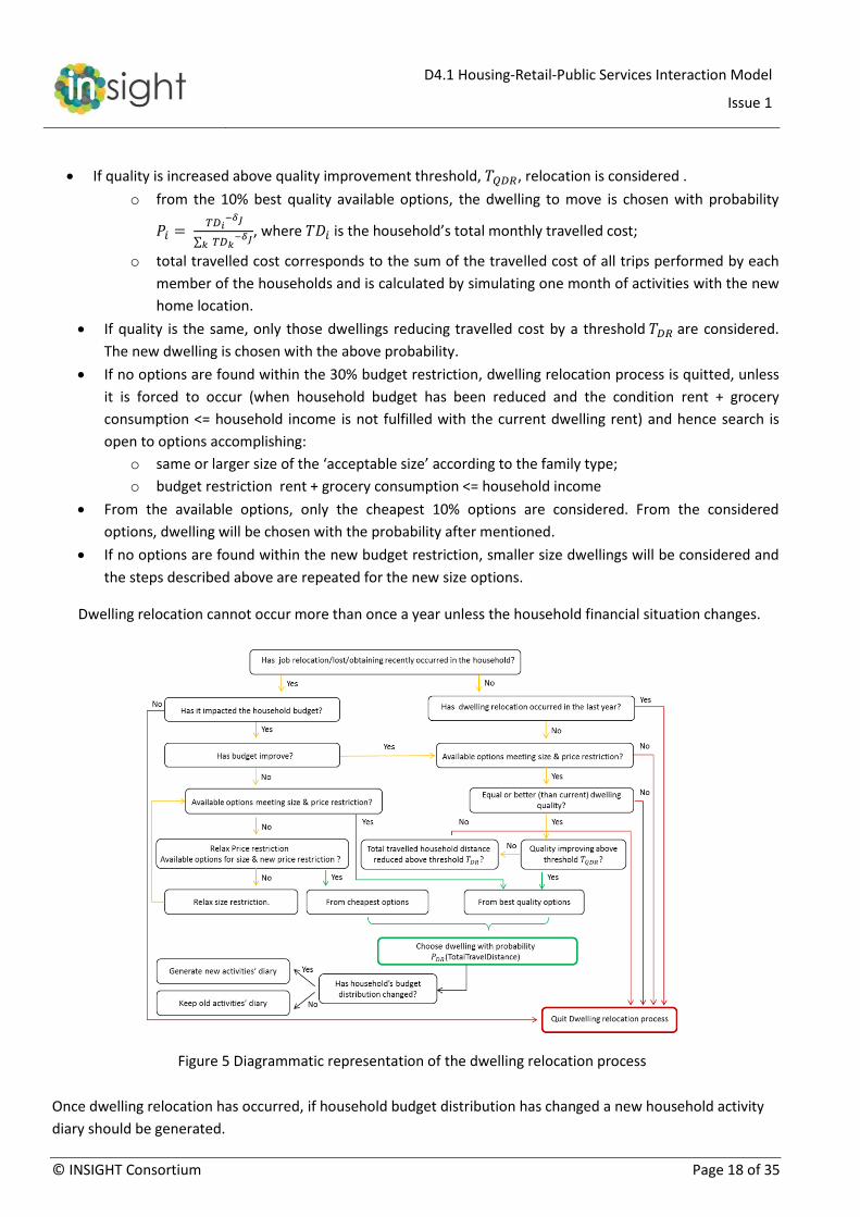
If quality is increased above quality improvement threshold, 𝑇𝑄𝐷𝑅, relocation is considered .
o from the 10% best quality available options, the dwelling to move is chosen with probability
𝑃𝑖 = 𝑇𝐷𝑖
−𝛿𝐽
∑ 𝑇𝐷𝑘−𝛿𝐽
𝑘
, where 𝑇𝐷𝑖 is the household’s total monthly travelled cost;
o total travelled cost corresponds to the sum of the travelled cost of all trips performed by each
member of the households and is calculated by simulating one month of activities with the new
home location.
If quality is the same, only those dwellings reducing travelled cost by a threshold 𝑇𝐷𝑅 are considered.
The new dwelling is chosen with the above probability.
If no options are found within the 30% budget restriction, dwelling relocation process is quitted, unless
it is forced to occur (when household budget has been reduced and the condition rent + grocery
consumption <= household income is not fulfilled with the current dwelling rent) and hence search is
open to options accomplishing:
o same or larger size of the ‘acceptable size’ according to the family type;
o budget restriction rent + grocery consumption <= household income
From the available options, only the cheapest 10% options are considered. From the considered
options, dwelling will be chosen with the probability after mentioned.
If no options are found within the new budget restriction, smaller size dwellings will be considered and
the steps described above are repeated for the new size options.
Dwelling relocation cannot occur more than once a year unless the household financial situation changes.
Figure 5 Diagrammatic representation of the dwelling relocation process
Once dwelling relocation has occurred, if household budget distribution has changed a new household activity
diary should be generated.

D4.1 Housing-Retail-Public Services Interaction Model
Issue 1
© INSIGHT Consortium Page 19 of 35
2.3.2 Retail agents
2.3.2.1 Attributes of the retail agents
It is possible to define as many types of retail as desired. For each type of retail, a set of properties has to be
defined (Table 7): possible retail sizes, retail jobs and retail salaries.
Retail sizes: e.g., 20, 40, 80 or 150 m2.
Retail jobs: the number of jobs offered by retail depends on the size of the retail (e.g. a small grocery of
40 m2 offers 4 jobs while one of 80 m2 may offer 6 jobs). Additionally, different jobs are classified
according to the minimum qualification required.
Retail salaries: the salaries depend on job qualification.
Table 7. Characteristics to define per retail type
Retail type / Properties
Sizes(m2) Retail jobs (number of jobs per size and qualification (Q) )
Salary
Retail_type_1 A B C D
Q1: A Q2: B
Q1: C Q2: D
Q1: E Q2: F Q3: G
Q1: H Q2: I Q3: J
Q1: salary_1 Q2: salary_2 Q3: salary_3
Retail_type_2 E F
Q1: K Q2: J
Q1: M Q2: N
Q1: salary_4 Q2: salary_5
… … … …
Retail_type_n H
Q1: Y Q2: Z
Q1: salary_m Q2: salary_n
Retail agents have the following attributes:
Type of retail: grocery, leisure, restaurants, etc.
Retail cell: cell where the retail is located.
Size.
Retail jobs: number of existing jobs classified by qualification and IDs of the persons that work there.
Retail count: number of visits in a month
2.3.2.2 Behaviour of the retail agents
Only long term decisions are considered for retail centres: opening and closure.
2.3.2.2.1 Retail closure
Every three months, each retail centre evaluates its performance (average monthly number of visits). If the
average monthly number of visits is less than the minimum number of visits required for success (see section
2.5), according to the business type and size, the business closes. The closure of the business destroys the jobs
associated to it and leaves free space for new retail activities to come. Employees should look for a new job. Job
search is performed first in the same kind of job offers (opening shops); if not successful, the search continues
among all other available jobs; finally if there is not success, a subsidy is requested to cover household basic
needs. The household financial situation is revisited and if the new household’s income is not sufficient to cover
dwelling and food costs, dwelling relocation occurs with probability P = 1.

D4.1 Housing-Retail-Public Services Interaction Model
Issue 1
© INSIGHT Consortium Page 20 of 35
2.3.2.2.2 Retail opening
In each area, if enough free space is available, every month new retail centres can be created. For each cell, a
list of the possible business types and size is built, and the first 50% of such list are created. The list is built as
follows:
The business of type and size with highest expected profitability within size and clients restrictions is
chosen:
o Size restriction: size should be equal or smaller than the free space in the area.
o Clients restrictions: for a given business type and size, the potential number of clients per square
meter should be higher than the minimum required. To calculate the number of clients per square
meter, the actual number of clients in the area of that business type is divided by the already
occupied area plus the occupied area by the new business.
#𝐶𝑙𝑖𝑒𝑛𝑡𝑠 𝑝𝑒𝑟 𝑚2 = # 𝐶𝑙𝑖𝑒𝑛𝑡𝑠 (𝑏𝑢𝑠𝑖𝑛𝑒𝑠𝑠 𝑡𝑦𝑝𝑒)
𝐶𝑚+𝑁𝑚 with 𝐶𝑚, the current occupied area for a given business
type and 𝑁𝑚 the new business’ size.
Expected profitability is defined as: 𝑃𝑟𝑜𝑓𝑖𝑡 = #𝐶𝑙𝑖𝑒𝑛𝑡𝑠 𝑝𝑒𝑟 𝑚2 ∗ 𝑁𝑚 .
If there are enough employees to open the new business, the business is added to the list.
Information about free space is updated and the process is repeated until no more options are
available.
Figure 6. Diagrammatic representation of retail closing process
Figure 7. Diagrammatic representation of retail opening process.
D4.1 Housing-Retail-Public Services Interaction Model
Issue 1
© INSIGHT Consortium Page 21 of 35
2.3.3 Public service agents
2.3.3.1 Attributes of the public service agents
The public service agent has a unique attribute which is the accessibility matrix. The accessibility matrix
represents the travel cost between any pair of cells.
2.3.3.2 Behaviour of the public service agents
Once a year the accessibility matrix is revisited and public transport policies can be applied to it to evaluate their
effect on qualitative changes on land use. These policies can be reactive or proactive. For instance the
accessibility to zones with higher number of jobs can be increased to attend the high transport demand, or the
opposite, accessibility to a lesser occupied area can be increased so as to foster job, housing or retail creation in
the area. Retail and households reaction to these policies are then measured in the coming year.
To account for the reaction of the accessibility to changes in the economic situation, accessibility is improved or
worsened in a proportion "alpha" to the decrements or increment of the unemployment rate. The resulting
accessibility matrix is defined as:
𝑁𝑒𝑤 𝑎𝑐𝑐𝑒𝑠𝑠𝑖𝑏𝑖𝑙𝑖𝑡𝑦𝑚𝑎𝑡𝑟𝑖𝑥 = 𝛼𝑐𝑢𝑟𝑟𝑒𝑛𝑡 𝑒𝑚𝑝𝑙𝑜𝑦𝑚𝑒𝑛𝑡 𝑟𝑎𝑡𝑒
𝑙𝑎𝑠𝑡 𝑦𝑒𝑎𝑟 𝑒𝑚𝑝𝑙𝑜𝑦𝑚𝑒𝑛𝑡 𝑟𝑎𝑡𝑒 𝑎𝑐𝑐𝑒𝑠𝑠𝑖𝑏𝑖𝑙𝑖𝑡𝑦𝑚𝑎𝑡𝑟𝑖𝑥
2.4 Exogenous variables
The exogenous variable considered in this model is the economic state of the system which we are representing
by the number of job offers. Job creation or destruction in the model occurs only in some explicitly considered
retail services. Jobs offer in industry, offices and other retail type correspond to exogenous variables. Changes in
the economic situation are modelled by creation or destruction of jobs in the sectors not explicitly considered
by the model.

D4.1 Housing-Retail-Public Services Interaction Model
Issue 1
© INSIGHT Consortium Page 22 of 35
2.5 Configuration and initialisation of the simulation model
Table 8 lists and explains the configuration parameters of the model
# Configuration Parameters
Description Example
Initialisation parameters
Cells parameters
[1] Types of cells Naming of the cell types Residential, Mix, Industrial
[2] Land use names Naming of the different types of land use
'residential, offices, retail, road network, green zones, school, hospital, other
equipment'
[3] Land use percentage Per each type of cell ([1]) the percentage of each type of land use ([2]) is provided
Residential: 40% residential, 2% offices, 8% retail, 20% road network, 8%
green_zones,10% school,10% hospital, 2% other equipment.
Mix: Residential: 25% residential, 5% offices, 5% retail, 30% road network, 5% green_zones,2% school,3% hospital, 5%
other equipment
[4] Cell side Side of the cell in meters 1000
[5] Number of cells
Number of cells in horizontal and vertical directions. Numbers shall be odd, in order to have a central cell as a reference.
horizontal cells = 25, vertical cells = 35
[6] Type of zones Naming of the types of zones zone_1 = Centre, zone_2 = urban, zone_3 =
outlying
[7] Zone distance
Distance (measured from the city centre) thresholds that define the different zones.
The number of values is equal to the number of zone types minus one. Distance shall be introduced in km.
Distance thresholds = [5,10] (for a scenario of 3 zones). If distance is lower than 5 the
cell will belong to zone 1, if distance is between 5 and 10 the cell will belong to
zone 2 and if distance greater than 10, cell will belong to zone 3.
[8] Cell type probability The cell types ([1]) depend on the zone types ([6]). For each zone type, the cell type is assigned probabilistically.
zone_1: 50% cell_type_1, 50% cell_type_2, 0% cell_type_3
Dwelling parameters
[9] Dwelling size Size of dwellings in square meters 60 m2, 80m2, 100m2
[10] Dwelling height Height of dwellings in meters 18 m

D4.1 Housing-Retail-Public Services Interaction Model
Issue 1
© INSIGHT Consortium Page 23 of 35
# Configuration Parameters
Description Example
[11] Dwelling percentages
The number of dwellings of each size ([9]) depends on the type of zone ([6]). In each zone, the square meters of dwellings are distributed among the different sizes according to a percentage.
zone_1 = 30% dwelling_size_1, 60% dwelling_size_2 ,10% dwelling_size_3
[12] Dwelling price
Dwelling price depends on zone type, size and quality. Type of zones ([6]) and dwelling sizes ([9]) are already defined by the user. For each pair (zone, size) the user can introduce as many different prices as desired, which is considered to be related with the 'quality' of the dwelling. Prices shall be introduced in Euros per month (€/month).
Dwelling price (zone_1,size_1, quality_1) = 900 euros/month
Dwelling price (zone_1, size_1, quality_2) = 1.500 euros/month
Dwelling price (zone_1, size_1, quality_3) = 2.500 euros/month
[13] Dwelling price percentage
Within each specific dwelling type (zone/size) the percentage of dwellings of each price (quality) shall be defined.
Dwelling price percentage (zone_1, size_1) = 50% 900 €/month, 30%
1.500€/month , 20% 2.500€/month
Office parameters
[14] Employees in offices Number of employees (job offer) per 100 m2 of office.
7 employees/100 m2
[15] Office salaries
The salary depends on the person qualification ([26]). For each person qualification a salary is defined. Salary shall be introduced in €/month.
salary(university) = 2.000 €/month, salary(school) = 1.200 €/month, ...
[16] Office salary percentage
Percentage of jobs per qualification 20% university, 60% non-university, 20%
school
Retail parameters
[17] Types of retails Types of retails ( grocery shall appear always as a possible type )
grocery, personal equipment, bars restaurants, leisure...
[18] Size of retails Size of the retail businesses in square meters per type of retail
grocery: 25 m2, 50 m2,100 m2
personal equipment: 40m2, 100 m2, 200 m2
bars restaurants: 80 m2, 120 m2, 200 m2
[19] Retail area built
Percentage x of initial retail area covered by existing retail businesses. 100-x will provide the empty area in which new retail businesses may be established.
80 %

D4.1 Housing-Retail-Public Services Interaction Model
Issue 1
© INSIGHT Consortium Page 24 of 35
# Configuration Parameters
Description Example
[20] Initial retail percentages
Percentage of available retail area ([19]) allocated to the different type of retail businesses.
grocery = 25 %
personal equipment = 25 %
bars restaurants = 50 %
[21] Retail jobs Number of jobs per retail type and size.
grocery(25 m2) = 2
grocery(50 m2) = 4
grocery(100 m2) = 10
personal equipment (100 m2) = 15
[22] Retail salary
Each type of retail has its own salaries. Within each type, different salaries are offered depending on the qualification ([26]) needed.
grocery(university) = 1.500 €/month
personal equipment (university) = 2.500 €/month
[23] Retail salary percentage
Percentage of retail jobs per qualification 10% university, 30% non-university, 60%
school
Public services
[24] Intrazonal distance factor
In order to measure intrazonal travel distance, the side of the cell is multiplied by an 'Intrazonal distance factor':
distance = cell side * Intrazonal distance factor
Intrazonal distance factor = 0.5 (if the cell side is 1000 m, the intrazonal distance is
500 m)
[25] accessibility factors
It is assume that accessibility between zones depends on the zone type of the origin and destination of the trip. For each pair of zone types, an accessibility factor is provided. The accessibility costs of travelling from cell_A to cell_B is equal to: distance(cell_A - cell_B) * accessibility factor (zone_type_A, zone_type_B)
accessibility factor (origin = zone_type_1, destination = zone_type_1) = 1.0
accessibility factor (origin = zone_type_1, destination = zone_type_2) = 1.5
Household
[26] People qualifications Naming of the qualification of the people school, non-university, university
[27] Adults in household Possible number of adults in a household (1,3) i.e. from 1 to 3
[28] Children in household Possible number of children per household. It is related with the number of adults.
1 adult household = (0,1) ----> Between 0 and 1 child is feasible
2 adults household = (0,3) ----> Between 0 and 3 children is feasible

D4.1 Housing-Retail-Public Services Interaction Model
Issue 1
© INSIGHT Consortium Page 25 of 35
# Configuration Parameters
Description Example
[29] Basic costs
Money spent per type of family and per type of retail. Grocery values are measured in €/month and the rest of the retail types in €.
Grocery money is used in the simulation to determine the minimum money a household needs to cover its basic needs during a month.
Other retail businesses ( personal equipment, bars restaurants...) money represents the money a household spends each time it goes to that retail type
grocery (2 adult / 1 child ) = 400 €/month
grocery (1 adult ) = 200 €/month
bars restaurants (1 adult ) = 25 €
[30] Adult factor
It is used to determine the number of adults to be created in the simulation. The simulation determines the minimum and the maximum number of adults compatible with the environment layer created. The number of agents for the simulation is defined as: minimum agents + adult factor * (maximum agents - minimum agents)
adult factor = 0 --> total adult population = minimum agents
adult factor = 1 --> total adult population = maximum agents
[31] Adult ages Adult range of ages 18, 65
[32] Children ages Children range of ages 0,17
Simulation parameters
Retail
[33] Minimum number of clients per business type and cost
The minimum number of clients a business needs to receive per month to be economically viable.
grocery(50 m2) = 357
grocery(500 m2) =2380
personal equipment (50 m2) = 157
personal equipment (500 m2) =1111
Household
[34] Percentage of relocating households
Percentage of the households that can consider relocation each month’s iteration. This percentage is decided by the model user.
5%
D4.1 Housing-Retail-Public Services Interaction Model
Issue 1
© INSIGHT Consortium Page 26 of 35
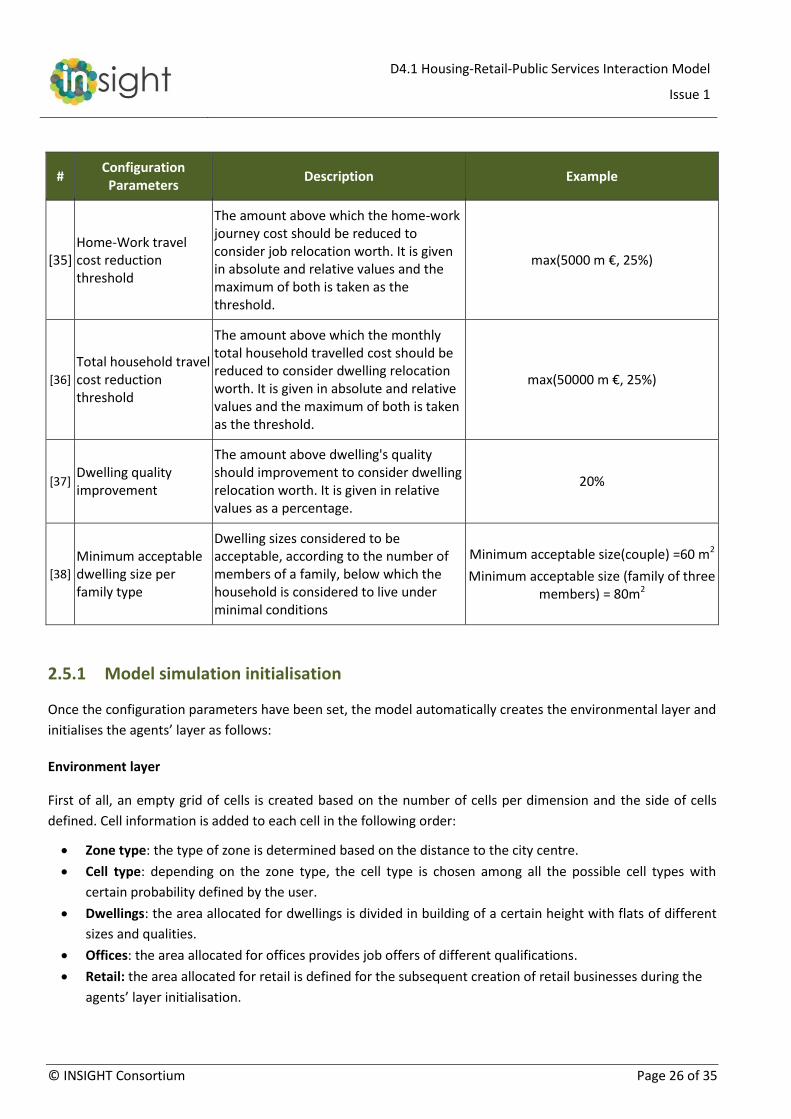
# Configuration Parameters
Description Example
[35] Home-Work travel cost reduction threshold
The amount above which the home-work journey cost should be reduced to consider job relocation worth. It is given in absolute and relative values and the maximum of both is taken as the threshold.
max(5000 m €, 25%)
[36] Total household travel cost reduction threshold
The amount above which the monthly total household travelled cost should be reduced to consider dwelling relocation worth. It is given in absolute and relative values and the maximum of both is taken as the threshold.
max(50000 m €, 25%)
[37] Dwelling quality improvement
The amount above dwelling's quality should improvement to consider dwelling relocation worth. It is given in relative values as a percentage.
20%
[38]
Minimum acceptable dwelling size per family type
Dwelling sizes considered to be acceptable, according to the number of members of a family, below which the household is considered to live under minimal conditions
Minimum acceptable size(couple) =60 m2
Minimum acceptable size (family of three members) = 80m2
2.5.1 Model simulation initialisation
Once the configuration parameters have been set, the model automatically creates the environmental layer and
initialises the agents’ layer as follows:
Environment layer
First of all, an empty grid of cells is created based on the number of cells per dimension and the side of cells
defined. Cell information is added to each cell in the following order:
Zone type: the type of zone is determined based on the distance to the city centre.
Cell type: depending on the zone type, the cell type is chosen among all the possible cell types with
certain probability defined by the user.
Dwellings: the area allocated for dwellings is divided in building of a certain height with flats of different
sizes and qualities.
Offices: the area allocated for offices provides job offers of different qualifications.
Retail: the area allocated for retail is defined for the subsequent creation of retail businesses during the
agents’ layer initialisation.
D4.1 Housing-Retail-Public Services Interaction Model
Issue 1
© INSIGHT Consortium Page 27 of 35
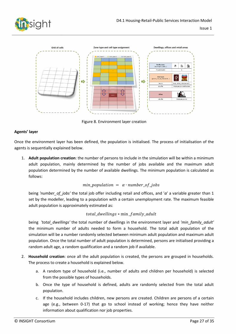
Figure 8. Environment layer creation
Agents’ layer
Once the environment layer has been defined, the population is initialised. The process of initialisation of the
agents is sequentially explained below.
1. Adult population creation: the number of persons to include in the simulation will be within a minimum
adult population, mainly determined by the number of jobs available and the maximum adult
population determined by the number of available dwellings. The minimum population is calculated as
follows:
𝑚𝑖𝑛_𝑝𝑜𝑝𝑢𝑙𝑎𝑡𝑖𝑜𝑛 = 𝛼 ∙ 𝑛𝑢𝑚𝑏𝑒𝑟_𝑜𝑓_𝑗𝑜𝑏𝑠
being 'number_of_jobs' the total job offer including retail and offices, and 'α' a variable greater than 1
set by the modeller, leading to a population with a certain unemployment rate. The maximum feasible
adult population is approximately estimated as:
𝑡𝑜𝑡𝑎𝑙_𝑑𝑤𝑒𝑙𝑙𝑖𝑛𝑔𝑠 ∗ min _𝑓𝑎𝑚𝑖𝑙𝑦_𝑎𝑑𝑢𝑙𝑡
being 'total_dwellings' the total number of dwellings in the environment layer and 'min_family_adult'
the minimum number of adults needed to form a household. The total adult population of the
simulation will be a number randomly selected between minimum adult population and maximum adult
population. Once the total number of adult population is determined, persons are initialised providing a
random adult age, a random qualification and a random job if available.
2. Household creation: once all the adult population is created, the persons are grouped in households.
The process to create a household is explained below.
a. A random type of household (i.e., number of adults and children per household) is selected
from the possible types of households.
b. Once the type of household is defined, adults are randomly selected from the total adult
population.
c. If the household includes children, new persons are created. Children are persons of a certain
age (e.g., between 0-17) that go to school instead of working; hence they have neither
information about qualification nor job properties.

D4.1 Housing-Retail-Public Services Interaction Model
Issue 1
© INSIGHT Consortium Page 28 of 35
d. The household salary is calculated as the sum of the salaries of the adults of the household.
e. The household searches for a feasible dwelling based on the household salary and the
household basic monthly costs (grocery costs). The money available for dwelling is calculated as:
𝑚𝑜𝑛𝑒𝑦_𝑎𝑣𝑎𝑖𝑙𝑎𝑏𝑙𝑒_𝑓𝑜𝑟_𝑑𝑤𝑒𝑙𝑙𝑖𝑛𝑔 = ℎ𝑜𝑢𝑠𝑒ℎ𝑜𝑙𝑑 𝑠𝑎𝑙𝑎𝑟𝑦 − 𝑏𝑎𝑠𝑖𝑐 𝑐𝑜𝑠𝑡𝑠
From all possible dwellings, the household selects one at random. If the money available does
not cover any dwelling rent and the basic household costs, a subsidy (€/month) is provided to
the household. When a subsidy is provided, the households are forced to select one of the
cheapest dwellings available, in order to minimise the subsidy to be provided. The income of
the household is calculated as the salary of each adult of the household plus the subsidy (if any).
f. Finally, the retail expenditure patterns of the household (i.e., in which retail businesses and
what amount is spent by the household) are defined. The money available after paying the
house rent and the basic costs is spent in retail businesses. The retail businesses where the
money is spent are assigned randomly. Note that the money spent per type of retail and type of
household every time a household visits the retail business is constant and set by the modeller
as a configuration parameter.
g. The process explained before is repeated until all the adults are assigned to a household.
Figure 9 shows the process of the population creation.
Figure 9. Agents layer initialisation process scheme
D4.1 Housing-Retail-Public Services Interaction Model
Issue 1
© INSIGHT Consortium Page 29 of 35
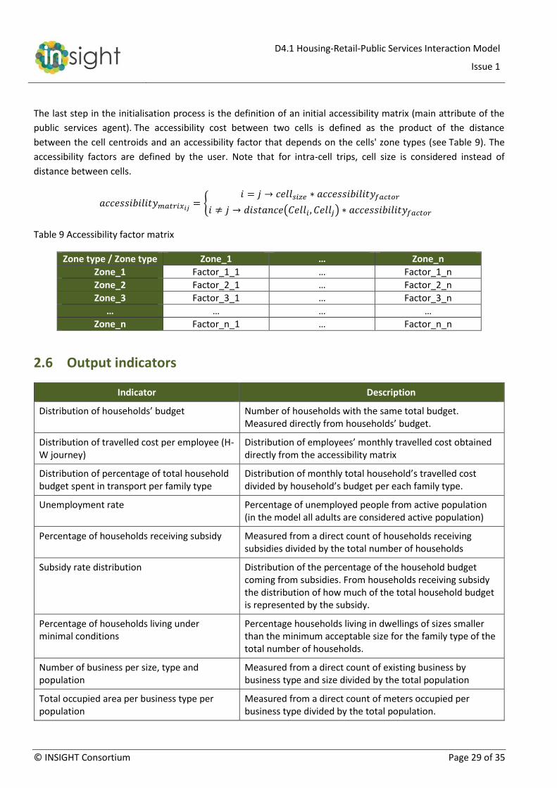
The last step in the initialisation process is the definition of an initial accessibility matrix (main attribute of the
public services agent). The accessibility cost between two cells is defined as the product of the distance
between the cell centroids and an accessibility factor that depends on the cells' zone types (see Table 9). The
accessibility factors are defined by the user. Note that for intra-cell trips, cell size is considered instead of
distance between cells.
𝑎𝑐𝑐𝑒𝑠𝑠𝑖𝑏𝑖𝑙𝑖𝑡𝑦𝑚𝑎𝑡𝑟𝑖𝑥𝑖𝑗= {
𝑖 = 𝑗 → 𝑐𝑒𝑙𝑙𝑠𝑖𝑧𝑒 ∗ 𝑎𝑐𝑐𝑒𝑠𝑠𝑖𝑏𝑖𝑙𝑖𝑡𝑦𝑓𝑎𝑐𝑡𝑜𝑟
𝑖 ≠ 𝑗 → 𝑑𝑖𝑠𝑡𝑎𝑛𝑐𝑒(𝐶𝑒𝑙𝑙𝑖 , 𝐶𝑒𝑙𝑙𝑗) ∗ 𝑎𝑐𝑐𝑒𝑠𝑠𝑖𝑏𝑖𝑙𝑖𝑡𝑦𝑓𝑎𝑐𝑡𝑜𝑟
Table 9 Accessibility factor matrix
Zone type / Zone type Zone_1 … Zone_n
Zone_1 Factor_1_1 … Factor_1_n
Zone_2 Factor_2_1 … Factor_2_n
Zone_3 Factor_3_1 … Factor_3_n
… … … …
Zone_n Factor_n_1 … Factor_n_n
2.6 Output indicators
Indicator Description
Distribution of households’ budget Number of households with the same total budget. Measured directly from households’ budget.
Distribution of travelled cost per employee (H-W journey)
Distribution of employees’ monthly travelled cost obtained directly from the accessibility matrix
Distribution of percentage of total household budget spent in transport per family type
Distribution of monthly total household’s travelled cost divided by household’s budget per each family type.
Unemployment rate Percentage of unemployed people from active population (in the model all adults are considered active population)
Percentage of households receiving subsidy Measured from a direct count of households receiving subsidies divided by the total number of households
Subsidy rate distribution Distribution of the percentage of the household budget coming from subsidies. From households receiving subsidy the distribution of how much of the total household budget is represented by the subsidy.
Percentage of households living under minimal conditions
Percentage households living in dwellings of sizes smaller than the minimum acceptable size for the family type of the total number of households.
Number of business per size, type and population
Measured from a direct count of existing business by business type and size divided by the total population
Total occupied area per business type per population
Measured from a direct count of meters occupied per business type divided by the total population.
D4.1 Housing-Retail-Public Services Interaction Model
Issue 1
© INSIGHT Consortium Page 30 of 35
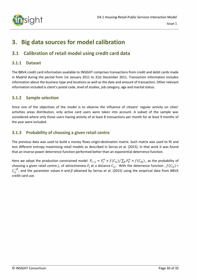
3. Big data sources for model calibration
3.1 Calibration of retail model using credit card data
3.1.1 Dataset
The BBVA credit card information available to INSIGHT comprises transactions from credit and debit cards made
in Madrid during the period from 1st January 2011 to 31st December 2011. Transaction information includes
information about the business type and locations as well as the date and amount of transaction. Other relevant
information included is client’s postal code, level of studies, job category, age and marital status.
3.1.2 Sample selection
Since one of the objectives of the model is to observe the influence of citizens’ regular activity on cities’
activities areas distribution, only active card users were taken into account. A subset of the sample was
considered where only those users having activity of at least 8 transactions per month for at least 9 months of
the year were included.
3.1.3 Probability of choosing a given retail centre
The previous data was used to build a money flows origin-destination matrix. Such matrix was used to fit and
test different entropy maximising retail models as described in Serras et al. (2015). In that work it was found
that an inverse power deterrence function performed better than an exponential deterrence function.
Here we adopt the production constrained model 𝑃𝑖→𝑗 = 𝐹𝑗∝ × 𝑓(𝐶𝑖𝑗)/ ∑ 𝐹𝑘
∝ × 𝑓(𝐶𝑖𝑘)𝑘 , as the probability of
choosing a given retail centre 𝑗, of attractiveness 𝐹𝑗 at a distance 𝐶𝑖𝑗. With the deterrence function , 𝑓(𝐶𝑖𝑗) =
𝐶𝑖𝑗−𝛽
, and the parameter values ∝ and 𝛽 obtained by Serras et al. (2015) using the empirical data from BBVA
credit card use.

D4.1 Housing-Retail-Public Services Interaction Model
Issue 1
© INSIGHT Consortium Page 31 of 35
3.2 Calibration of home and work choice model using mobile phone data
The distance to which agents are willing to travel from home to work every day is one of the key behavioural
variables of the toy model. Information about the travelled distance from home to work can be obtained from
data sources such as census or transport surveys; unfortunately, this information is expensive to obtain and it is
usually out of date (census and big transport surveys are usually conducted every 5-15 years). Mobile phone
data is an alternative to have this information updated at a fraction of the time and cost of traditional surveys
and usually providing bigger samples leading to more accurate results. Recent studies have shown the adequacy
of mobile phone data to identify home and work locations (see, e.g., Picornell et al., 2015; Isaacman et al.,
2011). The objective of this section to determine a realistic home-work distance distribution curve from mobile
phone data to calibrate home-work travel distances.
This section is structured as follows: first, the mobile phone dataset used is described; secondly, the
methodology followed to determine the home-work distance distribution is explained; thirdly, the results
obtained are shown; and finally the calibration process conducted is explained.
3.2.1 Dataset
The mobile phone data used for this study consists of a set of Call Detail Records (CDRs). CDRs are generated
when a mobile phone connected to the network makes or receives a phone call or uses a service (e.g., SMS,
MMS, etc.). For invoicing purposes, the information regarding the time and the Base Transceiver Station (BTS)
tower to which the user was connected when the call was initiated and ended is logged, providing an indication
of the geographical position of the user at certain moments. No information about the exact position of a user
in the area of coverage of a BTS is known. Also, no information about the location of the cell phone is known or
stored if no interaction is taking place. The CDRs were collected for Spain, comprising anonymous call
information for around 24 million users, accounting for more than 50% of the 2009 Spanish population. The
CDRs cover a period of time from September to November 2009 consisting of 53 days (including weekdays and
weekends) which provide more than 10 billion spatio-temporal registers. From the information contained in
each CDR, the following call information was extracted: caller’s anonymous ID, callee’s anonymous ID, day of
the call, time when the call starts, duration of the call, caller’s connected tower when the call starts and caller’s
connected tower when the call ends. Users’ positions are collected from BTS towers around Spain, leading to a
location accuracy of few hundreds of meters in urban areas and several kilometres in rural areas due to the
different density of towers. In order to preserve privacy, original records were encrypted. Additionally, all the
information presented in this paper is aggregated. No contract or demographic data were available for this
study. None of the authors of this study participated in the encryption or extraction of the CDRs.
3.2.2 Methodology: home-work distance distribution from mobile phone data
The methodologies presented in the literature to determine home and work locations from mobile phone data
are quite standard. The most common approach is to consider 'home' as the most frequently visited location
from XH p.m. y las YH a.m. Similarly, it is considered 'work' as the most frequently visited location from XW p.m.
y las YW p.m. For this study, the home interval selected ranges from 20 p.m. to 8 a.m. and the work interval
from 10 p.m. to 17 p.m. The home and work locations are determined at BTS level. It is assumed that home or
work coordinates are equivalent to BTS coordinates (reasonable hypothesis in high populated areas). The

D4.1 Housing-Retail-Public Services Interaction Model
Issue 1
© INSIGHT Consortium Page 32 of 35
distance between home and work is calculated as the Euclidean distance between those locations. Finally,
people are classified in 6 distance slots, leading to the following home-work distance distribution:
Group_1: People who travel between 0 and 5 Km
Group_2: 5 to 10 Km
Group_3: 10 to 15 Km
Group_4: 15 to 20 Km
Group_5: 20 to 50 Km
Group_6: More than 50 Km
3.2.3 Results: Home-work distance distribution for Madrid
For the study purposes, it is interesting to determine a home-work distance distribution of a specific city rather
than a general distribution of the whole country, hence, only a subset (specific city) of the whole dataset has
been used. The municipality of Madrid was chosen as an example, so as to take one realistic distribution for the
toy model. The home-work distance distribution of the municipality of Madrid is shown in figure X. It shows that
most of the people in the city (77 %) travel between 0 and 5 km to go to work. 10% of the population travel
between 5 and 10 Km., 5% travel between 10 and 20 km and the rest (around 5 %) travel more than 20 Km.
Figure 10. Home-work distance distribution of the municipality of Madrid
3.2.4 Calibration
The calibration process consists in identifying the proper utility function parameters that provide a home-work
distance distribution similar to the one obtained from mobile phone data. In order to compare both
distributions, a similarity indicator has been defined. The mathematical expression of the indicator is the
following:
∑ 𝛼𝑖 ∗ (𝐶𝐷𝑅_𝑣𝑎𝑙𝑢𝑒𝑖 − 𝑠𝑖𝑚𝑢𝑙𝑎𝑡𝑒𝑑_𝑣𝑎𝑙𝑢𝑒𝑖)2
𝑛
𝑖=1

D4.1 Housing-Retail-Public Services Interaction Model
Issue 1
© INSIGHT Consortium Page 33 of 35
being:
n: the number of distance slots consider in the distribution
alpha: factor that takes into account the importance of each slot. The importance is measure as
'people_in_the_slot/all_the_people'
CDR_value: Percentage of people in this slot according to mobile phone data
simulated_value: Percentage of people in this slot according to the simulation model
The objective of the home-work distance calibration process is to minimise this indicator, aiming to reproduce
the behaviour extracted from the CDRs.

D4.1 Housing-Retail-Public Services Interaction Model
Issue 1
© INSIGHT Consortium Page 34 of 35
4. Model capabilities
The model described in this document allows the evaluation of different scenarios impacting directly on one
sector and to trace the indirect effect on the others. Some examples are:
Polices affecting directly the transport services can be implemented in the model via the accessibility
matrix. The effect of these measures can be evaluated not only in the direct change of the travel cost but
also in the agents long term decisions such as the increment of population or retail density in given areas.
The effect of initial urban plans (percentage assigned to the different land uses: residential, offices, retail,
road network, green zones, school, hospital, etc.) in the final composition of the city and the spatial
distribution of different indicators related to socio-economic data, retail activity, etc.
Economic crisis scenarios can also be modelled, by observing the impact of the destruction of jobs in the
industrial sector (introduced as an exogenous variable) on the retail sector as well as on dwelling and jobs
relocations.
These three scenarios are currently been explored and tested with the model and will be used to explore in a
quick and flexible manner which are the more significant/relevant effects to be included in more fine-grained
models.

D4.1 Housing-Retail-Public Services Interaction Model
Issue 1
© INSIGHT Consortium Page 35 of 35
Annex I. References
Isaacman, S., Becker, R., Cáceres, R., Kobourov, S., Martonosi, M., Rowland, J., Varshavsky, A. “Identifying
important places in people’s lives from cellular network data.” Pervasive computing. Springer Berlin
Heidelberg, 2011. 133-151.
Picornell M., Ruiz T., Lenormand M., Ramasco J.J., Dubernet T., Frías-Martínez E. “Exploring the potential of
phone call data to characterize the relationship between social network and travel behavior”
Transportation 42, 2015. 647-668
Serras, J., Lenormand, M., Zachariadis V., Herranz, R., Fry, H., Ramasco, J.J., Cantu Ros, O.G., Batty, M. (2015)
“Observing shopping behaviour from credit card data” . Paper in preparation.
Timmermans, H.J.P. (2006) The saga of integrated land use and transport modelling: how many more dreams
before we wake up? In: Axhausen K (ed) Moving through nets: the physical and social dimensions of
travel. Elsevier, Oxford, pp 219–239
Wegener, M. (2004) Overview of land-use transport models. In: Hensher D, Button K (eds) Transport geography
and spatial systems. Pergamon/Elsevier Science, Kidlington, UK, pp 127–146